Impact of the Choice of Cross-Validation Techniques on the Results of Machine Learning-Based Diagnostic Applications

Abstract

Objectives

With advances in data availability and computing capabilities, artificial intelligence and machine learning technologies have evolved rapidly in recent years. Researchers have taken advantage of these developments in healthcare informatics and created reliable tools to predict or classify diseases using machine learning-based algorithms. To correctly quantify the performance of those algorithms, the standard approach is to use cross-validation, where the algorithm is trained on a training set, and its performance is measured on a validation set. Both datasets should be subject-independent to simulate the expected behavior of a clinical study. This study compares two cross-validation strategies, the subject-wise and the record-wise techniques; the subject-wise strategy correctly mimics the process of a clinical study, while the record-wise strategy does not.

Methods

We started by creating a dataset of smartphone audio recordings of subjects diagnosed with and without Parkinson’s disease. This dataset was then divided into training and holdout sets using subject-wise and the record-wise divisions. The training set was used to measure the performance of two classifiers (support vector machine and random forest) to compare six cross-validation techniques that simulated either the subject-wise process or the record-wise process. The holdout set was used to calculate the true error of the classifiers.

Results

The record-wise division and the record-wise cross-validation techniques overestimated the performance of the classifiers and underestimated the classification error.

Conclusions

In a diagnostic scenario, the subject-wise technique is the proper way of estimating a model’s performance, and record-wise techniques should be avoided.

I. Introduction

Healthcare informatics is a multidisciplinary field that has grown over the last few years. One of the main reasons for this growth is the integration of machine learning (ML) algorithms into clinical decision-making, with the goal of predicting diseases and assisting doctors in the diagnostic process. ML applications draw upon high-quality data recorded either using sophisticated equipment or wearable sensors and mobile devices. Research has shown that consumer-grade sensors embedded in smartphones, such as accelerometers, gyroscopes, and microphones, effectively detect digital biomarkers and have the potential to help researchers develop useful tools for the management and assessment of diseases [1].

In healthcare informatics research, most ML algorithms follow the supervised learning approach. First, a preprocessing algorithm extracts useful features from raw samples of subjects to create training and holdout sets. Each dataset forms a matrix of features and records with an additional class feature in the training set to designate whether a record belongs to a case or a control subject. Different classifiers are then trained on the training set, and their performance is measured on the holdout set. Only the classifiers that demonstrate model generalizability on unseen data are considered clinically useful. This data splitting process can be done in two different ways: subject-wise or record-wise. Subject-wise division ensures that the subjects in the training and holdout sets are independent. In other words, the records from each subject are assigned to either the training or the holdout set.

Contrarily, record-wise division splits the dataset randomly, without taking into account that the training set and the holdout set could share records from the same subjects. Measuring a model’s performance on a holdout set divided using the record-wise method can lead to incorrect reported performances. However, because medical datasets are not easy to obtain, it is not always possible to have a separate holdout set; thus, there is a need to estimate classifiers’ performance using cross-validation (CV) [2]. Researchers use various CV techniques, such as k-fold CV and leave-one-out CV, but choosing the wrong technique could lead to incorrect results, as many CV techniques simulate the record-wise division process. Furthermore, if a separate dataset is unavailable, the model’s generalizability cannot be demonstrated.

This paper aimed to illustrate how record-wise division can go wrong in a diagnostic scenario and how subject-wise division is the correct way to divide a dataset and estimate a model’s performance using CV. We demonstrated our hypothesis by creating a dataset from raw smartphone recordings to classify Parkinson’s disease (PD). We then split this dataset into training and holdout sets, using subject-wise and record-wise divisions. We estimated the performance of two pipelines—support vector machine (SVM) and random forest (RF)—using six CV techniques that simulated either subject-wise or record-wise behavior. A discussion is presented based on a comparison of the results.

The rest of the paper is organized as follows: Section 2 describes our methodology in detail, Section 3 presents the results, and Section 4 discusses the findings.

II. Methods

1. Dataset Creation

The database used in this study was collected from the mPower Public Research Portal [3,4]. mPower is a clinical study of PD performed only through a mobile application interface that consists of seven tasks to be completed by subjects, of which we were only interested in two (the demographic survey and the voice activity tasks). Our dataset was created in three phases: the acquisition of raw audio recordings, the choice of valid participants, and the extraction of audio features.

1) Data acquisition and subject filtering

To acquire the voice recordings, we used Python and SQL with the Synapse client [5]. The demographic survey was then used to separate subjects with PD (SWP) and healthy controls (HC).

Step 1: Subject filtering with the demographic survey

Subjects were classified as having PD if they were professionally diagnosed by a doctor; had a valid date of diagnosis; were parkinsonians (not caretakers); had never undergone surgery or deep brain stimulation to treat PD; and had a valid age. Subjects were said to be healthy if they were not professionally diagnosed by a doctor, had an invalid date of diagnosis, had no movement symptoms, and had a valid age.

Step 2: Subject filtering with the recording’s medical time point

In the voice activity task, subjects were asked to record their voice three times a day at a steady pace using the smartphone’s microphone, saying “Aaah” for 10 seconds. HC could record their voice at any time of the day, while SWP were required to record their voice at three specific times if they took PD medication: immediately before taking PD medication, immediately after taking PD medication, and at another time of the day. Otherwise, they could record their voices three times a day at any time. In this step, we kept only the recordings of subjects who did not take PD medication or recorded their voices before taking PD medications. Each of the selected subjects had a unique identifier (healthCode), which was used in step 3.

Step 3: Matched case-control study

In case-control clinical studies, researchers always aim to have an equal distribution of subjects to increase efficiency [6]. In this step, we evenly distributed the subjects of the two groups (SWP and HC). We selected only two recordings for each subject, as some subjects had many recordings, while others participated only once. Additionally, we analyzed each recording to ensure that we selected valid ones with minimal environmental noise. Furthermore, we matched the groups’ subjects by age and gender. We also selected subjects who were 40 years of age and older, as PD tends to affects more older individuals [7]. The final selected cohort is described in Table 1.

Table 1.

Final distribution of valid subjects in this study

	PD group	HC group	Total
Number of recordings	424	424	848
Number of subjects	212	212	424
Sex
Male	161	161	322
Female	51	51	102
Age (yr)	58.97±8.95 (40–79)	58.97±8.95 (40–79)

Values are presented as mean ± standard (min–max).

PD: Parkinson’s disease, HC: healthy controls.

2) Audio feature extraction

Feature extraction is an essential step in ML and pattern recognition systems [8], especially when dealing with audio data. Audio signals are non-stationary, and feature extraction is done on a frame basis by dividing the signals into short frames [9]. Using the pyAudioAnalysis [10] library, we extracted important audio features from the recordings, using short-term and mid-term processing techniques with a windowing procedure. All the recordings were sampled at 44.1 kHz and divided into short-term windows of 25 ms with a step size of 10 ms (usually between 20 and 40 ms [10]). This step generates a large matrix of features for each recording, making it necessary to apply the mid-term processing technique with a window of 4 seconds and a step size of 2 seconds (usually between 1 and 10 seconds [10]) to calculate feature statistics (feature_mean, feature_std, delta_feature_mean, delta_feature_std). Our dataset formed a data frame of 4,926 records × 139 features (Supplementary Tables S1 and S2).

3) Subject-wise and record-wise techniques

The objective of CV techniques is to assess the performance of predictive models in small datasets or when holdout data is unavailable for analysis [11]. This is often the case with medical datasets, which are often characterized by limited availability and limited subjects with repeated measurements, where each subject generates multiple samples (e.g., multiple audio recordings or X-ray scans and CT scans in image recognition problems). Furthermore, as these datasets are small, they are often used only during the training phase because limiting the size of the training data poses a risk of having a non-generalizable model. Thus, it is necessary to use CV to correctly estimate a model’s performance on unseen data.

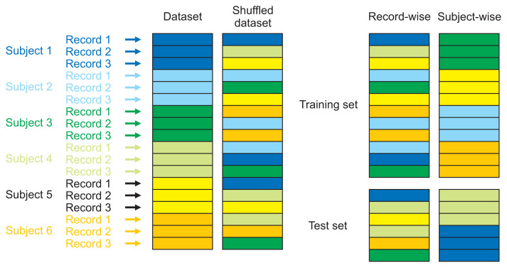
Before starting the classification of PD, we divided our dataset into two subsets (a training set and a holdout set) in two different ways: subject-wise division and record-wise division (Figure 1).

Figure 1.

Subject-wise and record-wise divisions.

Using the subject-wise division, the dataset was divided by the subjects’ healthCode, which means that the training set had different subjects than the holdout set. Since each subject had two recordings, this division ensured that each person’s recordings were either in the training set or in the holdout set. This division simulated the process of a clinical study. Using the record-wise division, the dataset was divided randomly into training and holdout sets, without considering that those sets could share recordings of the same subject. For data partitioning, we used 67% of the dataset as the training set and the remaining 33% as the holdout set in both subject-wise and record-wise divisions.

The training set was used with different CV techniques to estimate model performance on unseen data, and the holdout set was used to assess the performance of the models on separate unseen data by measuring the true classification error in both divisions. For CV, we used six techniques that are described in Table 2 [12,13].

Table 2.

Record-wise and subject-wise cross-validation (CV) techniques

CV group	CV technique	Description
Record-wise group	Stratified k-folds CV (skfcv)	With this technique, the dataset is divided into k blocks (folds) in a stratified manner [12]. One of the k blocks is selected as the validation set, while the remaining k–1 blocks constitute the training set. This process is repeated k times, with k = 10. As we are dealing with a binary classification problem, stratification is essential to ensure an equal distribution of both classes (persons with Parkinson’s disease and healthy controls) in each fold.
	Leave-one-out CV (loocv)	In this technique, only one record is left out for each learning process [12]. We consider n the number of records of our dataset, training is done on n-1 records, and validation is done on a single record. This process is repeated n times.
	Repeated stratified k-folds CV (rskfcv)	This technique is similar to stratified k-folds CV, but it is repeated n times [12]. We consider n the number of repetitions and k the number of blocks. This process is repeated k × n times, with k = 10 and n = 5. This method guarantees a more accurate estimate than without repetition.
Subject-wise group	Stratified-group k-folds CV (sgkfcv)	Using this technique, the dataset is divided into k blocks in a stratified manner with group of subjects [13]. This means that if a subject with a set of records is in block k, the recordings of that person do not occur in block k–1. One of the k blocks is chosen as the validation set, while the remaining k–1 blocks constitute the training set. This process is repeated k times, with k = 10.
	Leave-one-group-out CV (logocv)	In this technique, we leave out the records of only one group of subjects for each learning process [12]. We consider g the number of people in our dataset, learning is done on g–1 groups, and validation is done on a single group. This process is repeated g times.
	Repeated stratified-group k-folds CV (rsgkfcv)	This technique is similar to stratified-group-k-folds CV, but it is repeated n times [13]. We consider n the number of repetitions and k the number of blocks. This process is repeated k × n times, with k = 10, and n = 5. This method guarantees a more accurate estimate than without a repetition.

The CV techniques were organized into two groups. The subject-wise CV group simulated subject-wise division and included stratified-group k-folds CV, leave-one-group-out CV, and repeated stratified-group k-folds CV. The record-wise CV group included stratified k-folds CV, leave-one-out CV, and repeated stratified k-folds CV. The performance of the two groups is compared in the Results section.

2. Classification Models

1) Data pre-processing

Before starting the modeling phase, our dataset needed preprocessing in the form of data imputation and data scaling. In the data imputation step, missing values in a feature vector were replaced with the mean of the corresponding feature vector [14]. This step is essential since many classifiers, such as SVM, will not accept a dataset with missing values. Data scaling, in contrast, was used to normalize and standardize the dataset, as it contained different features with different scales. This step ensures that all the features contribute equally to the learning process.

2) Feature selection

Feature selection is one of the main concepts of ML. Having a large number of features in the dataset increases the complexity of the models and may reduce their performance. Various feature selection techniques are widely used in the literature [15], including analysis of variance and the Lasso and Ridge techniques. In this work, we used ElasticNet, which is a method combining the advantages of both the Lasso and Ridge techniques [12,16].

3) Machine learning workflow and pipelines

This study’s ML workflow was as follows: data imputation, data normalization and standardization, feature selection, and then classification. Repeating this process every time a CV technique is applied would be excessively time-consuming and lead to massive data leakage issues. To avoid this problem, we used pipelines. A pipeline is a way to automate the ML workflow, which is divided into independent modular parts that are reusable, making the models efficient and simplified and eliminating redundant work. In this study, we created two pipelines: the SVM pipeline and the RF pipeline; their hyperparameters were optimized using the randomized search technique (Table 3) [12,17].

Table 3.

Support vector machine (SVM) and random forest (RF) pipelines with their hyperparameters

SVM pipeline	Hyperparameters	RF pipeline	Hyperparameters
SVM_Pipeline = {  Imputation,  Normalization,  Standardization,  Fs_elasticnet,  SVM }	Imputation = {  Strategy = ‘mean’ } Normalization = {  Feature_range = (0,1) } Standardisation = {  with_mean = True,  with_std =True } Fs_elasticnet = { SelectFromModel { ElasticNet {  L1_ratio = 0.66,  alpha = 1.0 }}} SVM = {  kernel=‘rbf ‘,  gamma=‘scale’, C=0.30000000000000004, }	RF_Pipeline = {  Imputation,  Normalization,  Standardization,  Fs_elasticnet,  RF }	Imputation = {  Strategy = ‘mean’ } Normalization = {  Feature_range = (0,1) } Standardization = {  with_mean = True,  with_std = True } Fs_elasticnet = { SelectFromModel { ElasticNet { L1_ratio = 0.9, alpha = 1.0 }}} RF = { n_estimators=100, max_features=‘auto’, min_samples_split=2, min_samples_leaf=2, }

To compare the different CV techniques, we extracted a confusion matrix and calculated four performance measures to assess the pipelines’ performance: accuracy, sensitivity, specificity, and the F1-score (Table 4). The methodology is illustrated in Supplementary Figure S1.

Table 4.

Performance measures

Performance measure	Equation	Description
Accuracy	$\frac{\text{TP}+\text{TN}}{\text{TP}+\text{TN}+\text{FP}+\text{FN}}$	Accuracy is the proportion of correctly classified participants diagnosed with and without Parkinson’s disease among the total number of cases examined.
Sensitivity	$\frac{\text{TP}}{\text{TP}+\text{FN}}$	Sensitivity measures the proportion of participants diagnosed with Parkinson’s disease who have been correctly identified by the classifier.
Specificity	$\frac{\text{TN}}{\text{TN}+\text{FP}}$	Specificity measures the proportion of healthy participants who are correctly identified by the classifier.
F1 score	$\frac{2\text{TP}}{2\text{TP}+\text{FP}+\text{FN}}$	The F1 score is a measure of the accuracy of a test. It is calculated from the precision and the sensitivity of the test.

The following definitions are used in the equations:

True positive (TP) refers to the number of participants diagnosed with Parkinson’s disease who are correctly identified by the classifier.

True negative (TN) denotes the number of healthy participants who are correctly identified by the classifier.

False positive (FP) refers to the number of healthy participants who are incorrectly identified by the classifier.

False negative (FN) denotes the number of participants diagnosed with Parkinson’s disease who are incorrectly diagnosed by the classifier.

III. Results

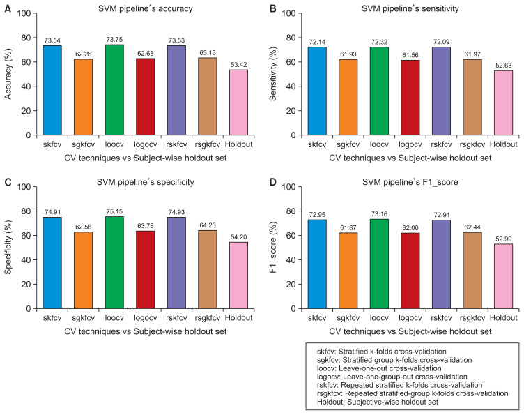
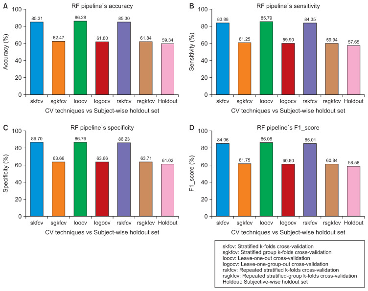
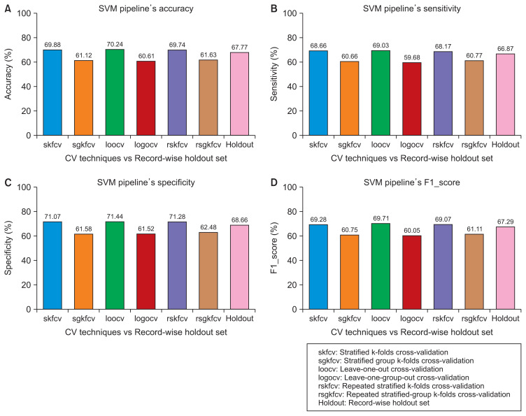
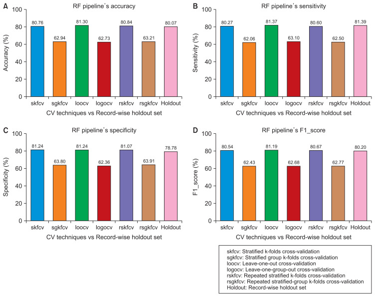
Figures 2 and 3 present the performance of the SVM and RF pipelines, respectively, with a dataset divided using subject-wise division. Figures 4 and 5 present the performance of SVM and RF pipelines, respectively, with the same dataset, but divided randomly using record-wise division.

Figure 2.

Performance of the support vector machine (SVM) pipeline with various cross-validation (CV) techniques compared to subject- wise division. (A) Accuracy. (B) Sensitivity. (C) Specificity. (D) F1 score.

Figure 3.

Performance of the random forest (RF) pipeline with various cross-validation (CV) techniques compared to subject-wise division. (A) Accuracy. (B) Sensitivity. (C) Specificity. (D) F1 score.

Figure 4.

Performance of the support vector machine (SVM) pipeline with various cross-validation (CV) techniques compared to record-wise division. (A) Accuracy. (B) Sensitivity. (C) Specificity. (D) F1 score.

Figure 5.

Performance of the random forest (RF) pipeline with various cross-validation (CV) techniques compared to record-wise division. (A) Accuracy. (B) Sensitivity. (C) Specificity. (D) F1 score.

1. Record-Wise Cross-Validation Group versus Subject-Wise Cross-Validation Group

Figures 2–5 show that the record-wise CV techniques out-performed the subject-wise CV techniques. For example, as shown in Figure 2, the accuracy of the SVM pipeline using the record-wise CV techniques was 73.54%, 73.75%, and 73.53% for stratified k-folds CV, leave-one-out CV, and repeated stratified k-folds CV, respectively. In contrast, the accuracy of the same pipeline using the subject-wise CV techniques was 62.26%, 62.68%, and 63.13% for stratified-group k-folds CV, leave-one-group-out CV, and repeated stratified-group k-folds CV, respectively. The same trends can be observed in the remaining figures with the RF pipeline and the four performance measures.

2. Record-Wise and Subject-Wise Cross-Validation Groups versus Subject-Wise Division

Although the record-wise CV techniques out-performed the subject-wise CV techniques using both pipelines, a comparison of the performance of those techniques with the performance of the same pipelines on unseen data with a subject-wise division showed that the record-wise CV techniques presented a much larger error (classification error) than the subject-wise CV techniques. For example, as shown in Figure 2, using the SVM pipeline with the four performance measures, the error between the record-wise CV techniques and the subject-wise division was approximately 20%, whereas the error between the subject-wise CV techniques and the same division was around 10%. The same trends can be observed in Figure 3, using the RF pipeline and the four performance measures, where the error between the record-wise CV techniques and the subject-wise division was more than 25%, while the error between the subject-wise CV techniques and the same division was approximately 3%.

3. Record-Wise and Subject-Wise Cross-Validation Groups versus Record-Wise Division

In this case, where the dataset was divided using record-wise division, the pipelines’ performance using the record-wise CV techniques was approximately equal to the performance of the pipelines on unseen data. For example, as shown in Figures 4 and 5, the error between the record-wise CV techniques and the record-wise division using the SVM and RF pipelines was approximately 2% and 1%, respectively, with the four performance measures. In the other case, as shown in the same figures, the pipelines’ performance using the record- wise division was higher than their performance using the subject-wise CV techniques. In terms of performance, the error between the record-wise division and the subject-wise CV techniques was approximately 7% and 17% for the SVM and RF pipelines, respectively.

IV. Discussion

What matters most in ML applications is the performance of the models on unseen data. CV techniques estimate the performance of those models, and by choosing inappropriate techniques, the classification error could be underestimated. The results showed that the record-wise CV techniques outperformed the subject-wise CV techniques in every case, although the latter techniques simulate the true process of a clinical study. From these results, we can conclude that subject-wise division is the correct way of dividing a medical dataset. This division ensures that the training set and the holdout set are subject-independent. The true reason for including a holdout set is to present the true error and show how each group of techniques estimates the performance of the pipelines. When dividing the dataset using subject-wise division, we observed a noticeable difference in error between the record-wise CV and the holdout set. This error is a sign of overfitting, which is caused by data leak-age. Record-wise CV techniques divide the dataset into training and validation sets by records, without taking into account the possibility that records of a given subject could be found in both the training set and the validation set; because the records of the same subject are correlated, the classifier does not only learn to classify the disease, but it also learns to identify the characteristics of each participant, thus overestimating the pipeline’s performance and underestimating the classification error. When dividing the dataset using the record-wise division, we observed that the performance of the pipelines on the holdout set was much higher than the performance of the subject-wise CV techniques, but this behavior is incorrect from a practical standpoint, as the performance of models on unseen data should always be lower than their estimated performance using CV. This behavior is a sign of underfitting, which results from data leakage from the beginning, caused by using an incorrect way of dividing the original dataset by records. Dividing the dataset using record-wise division could lead to an underestimation of classification error even on unseen data because the resulting holdout set from this division, in reality, does not represent unseen data due to the fact that records from the subjects in the training set leaked to the holdout set during the division process. Therefore, the classifier will not only learn to classify the disease, but also to identify the characteristics of each subject, and the difficult task of disease classification is replaced by the task of participant identification.

The results of the present study are supported by the findings of Saeb et al. [18], who used the Human Activity Recognition Dataset to assess how subject-wise and record-wise CV techniques estimated the RF classifier’s performance. This dataset contains samples of 30 subjects performing six tasks recorded using a smartphone’s accelerometer and gyroscope. Each subject had an average of 343 records, resulting in a dataset of 10,299 records. The results showed that record-wise CV overestimated the classification accuracy and underestimated the classification error compared to the subject-wise CV technique. By varying the number of folds from 2 to 30, the subject-wise CV error started at 27% and decreased to 7%. In contrast, the record-wise CV error started at 2% and remained steady even when the number of folds increased. Furthermore, those researchers carried out a systematic review of published studies that used CV techniques; they extracted 62 papers that met their chosen criteria and found that 45% of studies used record-wise CV techniques. They also found that the reported classification error of the subject-wise CV was more than twice that of the record-wise CV, reflecting incorrectly optimistic results from record-wise CV.

In the field of health informatics, CV techniques are widely used by researchers, and, as shown in this study, choosing the wrong technique could lead to a massive underestimation of the classification error, especially when a holdout set is unavailable to demonstrate the generalizability of a model. Based on this experiment, we present below the correct procedure for dealing with medical datasets.

• If the dataset is large enough to be divided into training and holdout subsets, one should use the subject-wise division technique. The training set and the holdout set must be subject-independent.

• Data preprocessing, feature selection, and model building should be grouped into pipelines to avoid data leakage.

• If the dataset is small, a subject-wise CV technique should be used to estimate model performance on unseen data. In Table 5, we present the execution time of each CV technique carried out using a 4 threads processing unit running at 1.9 GHz.

Table 5.

Execution times of the different cross-validation (CV) techniques

CV group	CV techniques	Execution time	Is the technique valid in this study?
Record-wise	Stratified k-folds CV	1 min	No
	Leave-one-out CV	6 hr 16 min 2 s	No
	Repeated stratified k-folds CV	4 min 49 s	No
Subject-wise	Stratified-group k-folds CV	1 min 10 s	Yes
	Leave-one-group-out CV	31 min 35 s	Yes
	Repeated stratified-group k-folds CV	4 min 59 s	Yes

We believe that this study will be of great interest to researchers and will serve as a reference for future works.

Supplementary Materials

Supplementary materials can be found via https://doi.org/10.4258/hir.2021.27.3.189.

References

- 1.Perry B, Herrington W, Goldsack JC, Grandinetti CA, Vasisht KP, Landray MJ, et al. Use of mobile devices to measure outcomes in clinical research, 2010–2016: a systematic literature review. Digit Biomark. 2018;2(1):11–30. doi: 10.1159/000486347. [DOI] [PMC free article] [PubMed] [Google Scholar]
- 2.Arlot S, Celisse A. A survey of cross-validation procedures for model selection. Stat Surv. 2010;4:40–79. [Google Scholar]
- 3.Bot BM, Suver C, Neto EC, Kellen M, Klein A, Bare C, et al. The mPower study, Parkinson disease mobile data collected using ResearchKit. Sci Data. 2016;3:160011. doi: 10.1038/sdata.2016.11. [DOI] [PMC free article] [PubMed] [Google Scholar]
- 4.Sage Bionetworks . The mPower Public Researcher Portal [Internet] Seattle (WA): Sage Bionetworks; 2019. [cited at 2021 Aug 3]. Available from: https://www.synapse.org/#!Synapse:syn4993293/wiki/247859. [Google Scholar]
- 5.Sage Bionetworks . Synapse REST API: Basics Table Query [Internet] Seattle (WA): Sage Bionetworks; 2016. [cited at 2021 Aug 3]. Available from: https://docs.synapse.org/rest/org/sagebionetworks/repo/web/controller/TableExamples.html. [Google Scholar]
- 6.Rose S, Laan MJ. Why match? Investigating matched case-control study designs with causal effect estimation. Int J Biostat. 2009;5(1):1. doi: 10.2202/1557-4679.1127. [DOI] [PMC free article] [PubMed] [Google Scholar]
- 7.Wong SL, Gilmour H, Ramage-Morin PL. Parkinson’s disease: prevalence, diagnosis and impact. Health Rep. 2014;25(11):10–4. [PubMed] [Google Scholar]
- 8.Khalid S, Khalil T, Nasreen S. A survey of feature selection and feature extraction techniques in machine learning. Proceedings of 2014 Science and Information Conference; 2014 Aug 27–29; London, UK. pp. 372–8. [Google Scholar]
- 9.Giannakopoulos T, Pikrakis A. Introduction to audio analysis: a MATLAB approach. San Diego, CA: Academic Press; 2014. [Google Scholar]
- 10.Giannakopoulos T. pyAudioAnalysis: an open-source python library for audio signal analysis. PLoS One. 2015;10(12):e0144610. doi: 10.1371/journal.pone.0144610. [DOI] [PMC free article] [PubMed] [Google Scholar]
- 11.Hawkins DM, Basak SC, Mills D. Assessing model fit by cross-validation. J Chem Inf Comput Sci. 2003;43(2):579–86. doi: 10.1021/ci025626i. [DOI] [PubMed] [Google Scholar]
- 12.Pedregosa F, Varoquaux G, Gramfort A, Michel V, Thirion B, Grisel O, et al. Scikit-learn: machine learning in Python. J Mach Learn Res. 2011;12:2825–30. [Google Scholar]
- 13.Github . Stratified GroupKFold [Internet] San Francisco (CA): Github.com; 2019. [cited at 2021 Aug 3]. Available from: https://github.com/scikit-learn/scikit-learn/issues/13621. [Google Scholar]
- 14.Kotsiantis SB, Kanellopoulos D, Pintelas PE. Data preprocessing for supervised leaning. Int J Comput Sci. 2006;1(2):111–7. [Google Scholar]
- 15.Chandrashekar G, Sahin F. A survey on feature selection methods. Comput Electr Eng. 2014;40(1):16–28. [Google Scholar]
- 16.Zou H, Hastie T. Regularization and variable selection via the elastic net. J R Stat Soc Series B Stat Methodol. 2005;67(2):301–20. [Google Scholar]
- 17.Wager S. Cross-validation, risk estimation, and model selection: comment on a paper by Rosset and Tibshirani. J Am Stat Assoc. 2020;115(529):157–60. [Google Scholar]
- 18.Saeb S, Lonini L, Jayaraman A, Mohr DC, Kording KP. The need to approximate the use-case in clinical machine learning. Gigascience. 2017;6(5):1–9. doi: 10.1093/gigascience/gix019. [DOI] [PMC free article] [PubMed] [Google Scholar]
Associated Data
This section collects any data citations, data availability statements, or supplementary materials included in this article.