Protocol for multimodal analysis of human kidney tissue by imaging mass spectrometry and CODEX multiplexed immunofluorescence

Summary

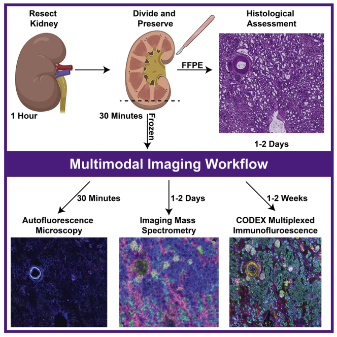
Here, we describe the preservation and preparation of human kidney tissue for interrogation by histopathology, imaging mass spectrometry, and multiplexed immunofluorescence. Custom image registration and integration techniques are used to create cellular and molecular atlases of this organ system. Through careful optimization, we ensure high-quality and reproducible datasets suitable for cross-patient comparisons that are essential to understanding human health and disease. Moreover, each of these steps can be adapted to other organ systems or diseases, enabling additional atlas efforts.

Graphical abstract

Highlights

• •Combines histology, imaging mass spectrometry, and multiplexed immunofluorescence
• •Describes workflows for producing high-quality data sets of the human kidney
• •Can be adapted to other organ systems or diseases

Here, we describe the preservation and preparation of human kidney tissue for interrogation by histopathology, imaging mass spectrometry, and multiplexed immunofluorescence. Custom image registration and integration techniques are used to create cellular and molecular atlases of this organ system. Through careful optimization, we ensure high-quality and reproducible datasets suitable for cross-patient comparisons that are essential to understanding human health and disease. Moreover, each of these steps can be adapted to other organ systems or diseases, enabling additional atlas efforts.

Before you begin

This specific protocol describes how to perform multimodal analysis on healthy, human tissue with the goal of constructing a cellular and molecular atlas of normal human tissues as part of the National Institutes of Health Human Biomolecular Atlas Program (HuBMAP) (Hu, 2019). These atlases require both co-registration and integration of many molecular and imaging assays so spatial comparisons can be made between samples. All the reagents you will need are in the key resources table. We have also successfully performed similar analyses on other human tissues, such as spleen and heart. Additional or different antibodies may be substituted depending on the application and organ. Moreover, these protocols have been developed using the specific instrumentation listed below and although they are applicable to similar instrumentation; certain parameters, such as spatial resolution and number of immunofluorescence cycles, will need to be adjusted based on individual platform limitations.

Key resources table

REAGENT or RESOURCE	SOURCE	IDENTIFIER
Antibodies
CD7 (1/200 dilution)	Akoya Biosciences	4150022
Aquaporin 1 (1/200 dilution)	Abcam	ab9566
Aquaporin 2 (1/200 dilution)	Abcam	ab230170
CD90 (1/200 dilution)	Akoya Biosciences	4150021
CD38 (1/200 dilution)	Akoya Biosciences	4150007
Ki67 (1/200 dilution)	Akoya Biosciences	4250019
Nestin (1/200 dilution)	Abcam	ab221660
CD45 (1/200 dilution)	Akoya Biosciences	4150003
Uromodulin (1/200 dilution)	Abcam	ab207170
ß-Catenin (1/200 dilution)	Abcam	ab32572
Vimentin (1/200 dilution)	Abcam	ab92547
PARP1 (1/200 dilution)	Abcam	ab191217
CD31 (1/200 dilution)	Akoya Biosciences	4250009
CD93 (1/200 dilution)	Abcam	ab134079
E-Cadherin (1/200 dilution)	Cell Signaling Technology	3195S
Laminin (1/200 dilution)	DSHB	2E8
KDR/Vegf 2 (1/200 dilution)	Abcam	ab237634
Calbindin (1/200 dilution)	Abcam	ab108404
Cytokeratin 7 (1/200 dilution)	Abcam	ab68459
α-Smooth Muscle Actin (1/200 dilution)	Abcam	ab7817
Renin (1/200 dilution)	Abcam	ab212197
Tryptase (1/200 dilution)	Abcam	ab151757
MARCKS (1/200 dilution)	Abcam	ab184546
CODEX Barcodes	N/A	N/A
RX025 (1/200 dilution)	Akoya Biosciences	6450009
RX002 (1/200 dilution)	Akoya Biosciences	6250001
RX015 (1/200 dilution)	Akoya Biosciences	6350003
RX022 (1/200 dilution)	Akoya Biosciences	6150008
RX035 (1/200 dilution)	Akoya Biosciences	6250010
RX033 (1/200 dilution)	Akoya Biosciences	6350008
RX007 (1/200 dilution)	Akoya Biosciences	6150003
RX026 (1/200 dilution)	Akoya Biosciences	6250007
RX024 (1/200 dilution)	Akoya Biosciences	6350005
RX001 (1/200 dilution)	Akoya Biosciences	6150001
RX047 (1/200 dilution)	Akoya Biosciences	6250012
RX042 (1/200 dilution)	Akoya Biosciences	6350010
RX013 (1/200 dilution)	Akoya Biosciences	6150005
RX032 (1/200 dilution)	Akoya Biosciences	6250009
RX006 (1/200 dilution)	Akoya Biosciences	6350002
RX016 (1/200 dilution)	Akoya Biosciences	6150006
RX023 (1/200 dilution)	Akoya Biosciences	6250006
RX004 (1/200 dilution)	Akoya Biosciences	6150002
RX005 (1/200 dilution)	Akoya Biosciences	6250002
RX021 (1/200 dilution)	Akoya Biosciences	6350004
RX010 (1/200 dilution)	Akoya Biosciences	6150004
RX014 (1/200 dilution)	Akoya Biosciences	6250003
RX027 (1/200 dilution)	Akoya Biosciences	6350006
Biological samples
Human kidney	Vanderbilt Medical Center CHTN	N/A
Chemicals, peptides, and recombinant proteins
Dimethyl sulfoxide, ReagentPlus, ≥99.5%	Sigma-Aldrich	D5879-4L
Poly-L-lysine solution, 0.1% (w/v) in H2O	Sigma-Aldrich	P8920-500ML
10× CODEX Buffer	Akoya Biosciences	7000001
CODEX Assay Reagent	Akoya Biosciences	7000002
Dumont Cover Slip Forceps Dumoxel	Fine Science Tools	11251-33
4% Formaldehyde, methanol-free	Thermo Fisher Scientific	R37814
Methanol-free Formaldehyde Ampules	Thermo Fisher Scientific	28908
Ambion Nuclease-Free Water	Thermo Fisher Scientific	43–879-36
96-Well plates	Akoya Biosciences	7000006
Molecular probes DAPI (4′,6 Diamidino 2 Phenylindole, Dihydrochloride)	Thermo Fisher Scientific	D1306
CODEX Gaskets v2	Akoya Biosciences	7000010
Carboxymethylcellulose sodium salt, medium viscosity	Sigma-Aldrich	C4888-500G
2-Methylbutane, Reagent Grade, ≥99%	Fisher Scientific	60048070
Disposable aluminum dishes	Fisher Scientific	S40284
2′,5′-Dihydroxyacetophenone, 97%	Sigma-Aldrich	D107603-25G
Methanol, for HPLC, ≥99.9%, CAS 67-56-1, Sigma-Aldrich 34860-4X4L-R	Sigma-Aldrich	34860-4X4L-R
Acetone, HPLC Plus, for HPLC, GC, and residue analysis, ≥99.9%	Sigma-Aldrich	650501-4X4L
Tetrahydrofuran, inhibitor-free, for HPLC, ≥99.9%,	Sigma-Aldrich	34865
16% Paraformaldehyde	Electron Microscopy Sciences	15710
Ethanol, 99.5%	Fisher Scientific	AC615095000
Xylenes	Fisher Scientific	X5-500
Ammonium hydroxide	Fisher Scientific	A669S-500
TRIzol Reagent	Thermo Fisher Scientific	15596026
1× Phosphate-Buffered Saline	Life Technologies	14190144
RLT Buffer Plus	QIAGEN	1053393
RNeasy MinElute Cleanup Kit	QIAGEN	74204
RPE Buffer	QIAGEN	1018013
2-Mercaptoethanol	Fisher Scientific	21985023
Cryoseal	Fisher Scientific	22050262
Poly-L-lysine 0.1%	Sigma-Aldrich	P8920
Paraffin	Fisher Scientific	23021750
Periodic Acid and Schiff Reagent	Abcam	Ab150680
Hematoxylin	Fisher Scientific	22050198
Nuclease-Free Water	Thermo Fisher Scientific	AM9938
DEPC-Treated Water	Thermo Fisher Scientific	4387937
10% Buffered Formalin Phosphate	Fisher Scientific	SF100-4
Glycogen	Thermo Fisher Scientific	AM9510
Other
Indium tin oxide-coated glass slides	Delta Technologies	CG-81IN-S115
Anti-roll Bar	Leica	14047742497
Bent-tip tweezers	Fine Science Tools	11251-33
6-Well TC Plates	VWR	10861-554
Phase Lock Gel - Heavy	Quantabio	2302830
Cryostat Blade	Electron Microscopy Systems	63059-25
27G Precisionglide needles	BD	305109
Embedding molds	Thermo Fisher Scientific	1841
50 kDa MWCO filter	EMD Millipore	UFC505096
TM Sprayer M3	HTX Imaging	N/A
Bruker timsTOF Pro	Bruker	N/A
Axio Scanner Slide Scanner	Carl Zeiss AG	N/A
Axio Observer	Carl Zeiss AG	N/A
CODEX System	Akoya Biosciences	N/A
Flatbed Scanner	Epson	B11B175012
Critical commercial assays
CODEX Conjugation Kit	Akoya Biosciences	7000009
CODEX Staining Kit	Akoya Biosciences	7000008
Deposited data
Highly Multiplexed Immunofluorescence of the Human Kidney using Co-Detection by Indexing (CODEX)	N/A	10.1101/2020.12.04.412429
Next Generation Histology-Directed Imaging Mass Spectrometry Driven by Autofluorescence Microscopy	N/A	10.1021/acs.analchem.8b02885
Advanced Registration and Analysis of MALDI Imaging Mass Spectrometry Measurements through Autofluorescence Microscopy	N/A	10.1021/acs.analchem.8b02884
Software and algorithms
FIJI ImageJ	https://fiji.sc	N/A
regToolboxMSRC	https://github.com/nhpatterson/regtoolboxmsrc	N/A
Cardinal	https://cardinalmsi.org	N/A
LipidMAPS	https://www.lipidmaps.org/	N/A

CRITICAL: Freeze thaw cycles quickly degrade many reagents, such as antibodies. In general, we recommend aliquoting out single use volumes of these reagents. If this is not possible, we recommend leaving these reagents within the refrigerator once they are thawed.

Step-by-step method details

Collection and stabilization of human kidney tissue after surgical excision

Timing: 1 h

This portion of the protocol enables collection and stabilization of human kidney tissue after key clinical diagnostic workup. Assessments are made for experimental pathological assessment and multimodal analysis. Human kidney tissue was surgically removed during a full nephrectomy and remnant tissue was processed for research purposes by the Cooperative Human Tissue Network at Vanderbilt University Medical Center. Remnant biospecimens were collected in compliance with the Cooperative Human Tissue Network standard protocols and National Cancer Institute’s Best Practices for the procurement of remnant surgical research material. Participants were consented for remnant tissue collection in accordance to institutional IRB policies.

• 1.
  Prepare the kidney tissue for freezing.

  • a.
    De-identified human kidney tissues are collected from surgical resections selected based on patient and clinical metadata (e.g., specific age range). All patients must have consented to allow their tissue to be used for research purposes.
  • b.
    Cut the kidney in half coronally, generally the longest plane (Figure 1A).
  • c.
    Cut out a portion of the kidney (∼80 × 60 × 4 mm) that is farthest away from tumor or diseased areas using a scalpel or other blade (Figure 1B).

    • i.
      Photograph the smaller piece of kidney in reference to its original location within the entire kidney (Figure 1B).
    • ii.
      Smaller or larger tissue pieces can be extracted depending on the original size of the organ, tumor location, and desired number of samples. The size of the pieces that require embedding are essential for proper freezing.
  • d.
    Further cut the piece of kidney into 3–5 smaller pieces (∼2 × 15 × 4 mm, Figure 1C).

    CRITICAL: Larger kidney resections result in freezing artifacts from uneven freezing between the outside and the center of the tissue. To prevent this, we recommend freezing tissues that are ∼2 × 15 × 4 mm or smaller.

    • i.
      Photograph the smaller pieces to reference how they were cut so that the smaller pieces that are frozen and embedded can be traced back to the larger organ (Figure 1C).
    • ii.
      Each of these pieces will later be cut in half, where one half will be fresh frozen (Step 2) and the other formalin fixed and paraffin embedded (FFPE) (Step 3).

Figure 1.

Kidney resections

Section of resected kidney with the superior and inferior poles labeled.

(A) Whole kidney cut in half, coronally with superior and inferior poles labeled (black dotted line).

(B) A portion of the kidney (∼80 × 60 × 4 mm) that is farthest away from the tumor (green dotted line).

(C) The extracted portion is divided into thirds or fourths to ensure event freezing (blue dotted line).

• 2.
  The stabilization and freezing procedure for fresh frozen tissue blocks.

  • a.
    Place a layer of dry ice into a freezer box and add enough isopentane to make a slurry.
  • b.
    Remove kidney tissue blocks from plastic encasing and measure the weight, length, width, and height (Figure 2).
  • c.
    Place a metal weigh boat on top of the isopentane slurry and let cool.
  • d.
    Write the sample number and orientation onto mold edges, indicating inner/outer and superior/inferior edges (Figure 3).
  • e.
    Add tissue to the metal boat and wait until the tissue is completely frozen.
  • f.
    Add enough 2.6% carboxymethylcellulose (CMC) to cover the bottom of the embedding mold.

    Note: CMC is used as an embedding material rather than more common embedding materials, such as optimal cutting temperature (OCT) compound, to avoid introducing chemical interferences during MS analysis (Stoeckli et al., 2007). While other embedding materials are compatible for IMS (Gill et al., 2017, Strohalm et al., 2011), they require optimization and testing compatibility with different methodologies.

  • g.
    Place the embedding mold with CMC on top of the isopentane slurry.

    • i.
      Wait until CMC starts to freeze and begins to turn opaque (Figure 4, center).
  • h.
    Place tissue onto freezing CMC layer and slowly add more CMC until the tissue is completely covered (Figure 4, left).
  • i.
    When completely frozen, wrap in foil, label, and store at −80°C.

    Note: Foil has a lower specific heat than other storage containers (e.g., plastic) so this prevents freeze/thaw artifacts from uneven cooling/freezing. This is most important right after freezing.

Figure 2.

Measurement guide

Measure and record the length, width, and thickness of the kidney tissue pieces using gridded paper (as shown above) or other instruments.

Figure 3.

Kidney embedding and freezing

(A–D) (A) Label mold such that orientation of the kidney can be maintained. Images of unfrozen tissue (B), partially frozen tissue and CMC (C), and CMC embedded tissue ready for storage (D).

Figure 4.

Schiff’s reagent stain example

(A) Tissue after incubation with periodic acid. The tissue is clear and uncolored.

(B) Tissue appearance after incubation with Schiff’s reagent. The tissue is light pink.

(C) Tissue appearance after exposure to warm water. The tissue turns bright pink when exposed to warm water.

• 3.
  Fixing and embedding procedure for FFPE tissue.

  • a.
    Carefully place a non-frozen piece of tissue into an embedding cassette with the cut side facing down and submerge in a 10% neutral-buffered formalin solution for at least 12 h but typically 18 h.

    • i.
      The tissue can be left in fixative for up to 24 h, although this will vary based on tissue type and thicknesses.
  • b.
    Move the tissue cassettes into 70% ethanol for 35 min.
  • c.
    Submerge the tissue into 90% ethanol for 35 min.
  • d.
    Submerge the tissue in 95% ethanol for 35 min.
  • e.
    Submerge the tissue into three sequential containers of 100% ethanol, each for 35 min.
  • f.
    Submerge the tissue in 100% xylenes for 35 min, three times (total of 105 min). Fresh xylene solutions are required for each separate submersion.
  • g.
    Submerge the tissue in paraffin (wax) for 60 min, three times (total of 3 h).
  • h.
    The tissue is then embedded with additional paraffin at ∼20°C (room temperature) to make a block such that the tissue is entirely encased.

Pathological assessment of PAS-stained FFPE tissues

Timing: 1–2 days

By the end of this major step, a representative histological stain of a human kidney tissue section is assessed for normalcy by a pathologist prior to multimodal imaging. After pathological assessment, each tissue can be classified by proportion of medulla and/or cortex, disease, or artifacts.

• 4.
  Procedure for periodic acid-Schiff (PAS) staining of FFPE tissues for histological assessment (adapted from Munro, 1971).

  Note: Hematoxylin and eosin or other histological staining procedures can be used instead of a PAS stain and may be preferred for other tissue types. PAS is optimal for kidney assessment, as it allows assessment of proximal tubular brush borders and other kidney structures. Specific histological stains may be optimal for specific tissues and an expert pathologist should be consulted before choosing a staining procedure.

  • a.
    At the beginning of the staining process, staining reagents should be equilibrated to ∼20°C (room temperature) from refrigerator storage.
  • b.
    Deparaffinize tissue by submerging in xylenes for 3 min, twice. The wax should be removed, and the tissue should look transparent. Additional washes can be incorporated as needed for complete paraffin removal.
  • c.
    Rehydrate the tissue using graded alcohol solutions and distilled water.

    • i.
      Begin by submerging in 100% ethanol for 1 min, twice.
    • ii.
      Submerge the tissue in 95% ethanol for 1 min.
    • iii.
      Submerge the tissue in 70% ethanol for 1 min.
    • iv.
      Submerge the tissue in 100% water for 1 min.
  • d.
    Rinse the tissues with generous amounts of distilled water.
  • e.
    Incubate the tissue in 0.5% periodic acid in distilled water for 10 min for tissue oxidation.

    Note: The periodic acid solution can be reused for ∼1 month before needing to be replaced.

  • f.
    Rinse the tissues generously with distilled water.
  • g.
    Incubate the tissues in Schiff’s reagent for 30 min.

    Note: Different tissue types require different incubation times, generally ranging from 15–30 min.

    • i.
      The Schiff’s reagent can be reused for ∼1 month before needing to be replaced.
  • h.
    Rinse the tissues in generous amounts of warm (∼40°C) water.

    • i.
      While distilled water is preferred, heated tap water is sufficient for this step.
    • ii.
      The tissue should appear pink after rinsing with warm water (Figure 4C).
  • i.
    Counterstain the tissue in hematoxylin for 1 min and rinse generously with distilled water.
  • j.
    Dip the tissue section into 0.5% ammonium hydroxide a single time and rinse with generous amounts of distilled water.

    • i.
      The tissue should be rinsed until the runoff water is colorless.
  • k.
    Dehydrate the tissue using graded alcohol solutions.

    • i.
      Dip the tissue 10 times for ∼ 1 s into 95%, 95%, 100%, and 100% ethanol solutions, sequentially, with ten dips for each different solution.
    • ii.
      If the last 100% ethanol rinse is colored by residual stain, additional washing in new 100% ethanol solution should be performed.
  • l.
    Submerge the tissue in xylenes for 1 min, twice.
  • m.
    Coverslip the tissues for long term storage and higher quality microscopy.

    • i.
      Dip the tissue in xylenes, remove slide and hold horizontally and add 2–3 drops of cytoseal to the tissue surface.
    • ii.
      Line up the slide and cover slip before slowly placing the coverslip on the slide.
    • iii.
      If needed, use a dissecting tool or other pointed object to remove/displace bubbles from the tissue by gently pressing down on the cover slip.

      CRITICAL: Any bubbles between the tissue and coverslip will prevent acquisition of high-quality microscopy images.

  • n.
    Image slides using a Leica brightfield scanner (or equivalent) at 20× (∼1 μm spatial resolution) and save the file.

• 5.
  Histological assessment of FFPE tissue for determining tissue architecture, disease, and normalcy.

  • a.
    Determine the percentage of cortex, medulla, renal pyramids, and renal pelvis within the tissue section.

    • i.
      Determine the presence or absence of kidney diseases or sampling degradation, such as autolysis or non-renal diseases (e.g., cancer).
    • ii.
      Assess the severity of common renal diseases (0–3, None-Severe), such as glomerular or tubulointerstitial diseases.

Sample preparation for multimodal workflows

Timing: 1–3 days

This protocol describes cryosectioning, microscopy, and RNA assessment in preparation for and prior to samples entering the multimodal workflow.

• 6.
  Cryosection fresh frozen tissue onto a glass slide or coverslip for different analytical workflows.

  • a.
    Set the internal temperature of the cryostat to −21°C and object temperature to −20°C.
  • b.
    Clean the blade with ethanol and a lint free wipe to remove potential chemical contaminants before placing the blade into the cryostat.
  • c.
    Mount the CMC embedded tissue onto a cold chuck using OCT. Take care to avoid OCT touching the tissue directly, and only contact the CMC shell.

    • i.
      A flat surface can be shaved onto the mounting surface using a razor blade to ensure correct orientation and enhanced tissue block adherence.

      CRITICAL: OCT causes significant ion suppression during mass spectrometry analysis. Tissue that directly touches OCT should be discarded.

  • d.
    Adjust angle of sectioning stage (Figure 5) to ensure quality sectioning.

    • i.
      Poor angle adjustment causes CMC embedding to fragment and lose structural integrity during sectioning. The angle adjustment depends on the flatness and orientation of the tissue as well as the blade that is used. This will need to be optimized for procedure.
  • e.
    Trim the CMC shell using 30–50 μm step increments until the tissue becomes visible.

    • i.
      The blade often dulls during this trimming step and may need to be replaced for high-quality and/or serial sections.
    • ii.
      Excess CMC surrounding the tissue may be removed with a cooled razor blade to reduce section size and improve sectioning.
  • f.
    Adjust the section thickness setting to 10 μm and section until the portion of the tissue for multimodal analysis is reached, this often is when the entire tissue face is cut, rather than part or portion of the tissue face.
  • g.
    Position the anti-roll bar, such that it is ahead of the blade, but does not scrape the tissue.

    • i.
      If the anti-roll bar is too far forward it scrapes the tissue, but if it is pulled back too far, the tissue section will roll and fold during sectioning.
  • h.
    Section until the desired number of tissue sections are acquired (at least one for each modality although multiple sections for modality may be beneficial for technical replicates). Manipulate sections onto slides with a fine tipped paint brush and thaw mount using a gloved hand and then place mounted, cut tissue on a 20°C hot plate for 30 s.

    • i.
      Imaging mass spectrometry analysis requires mounting onto indium tin oxide coated slides or another conductive substrate.
    • ii.
      CODEX immunofluorescence analysis requires mounting onto poly-lysine coated coverslips.
  • i.
    Tissue sections should be stored in a desiccator if undergoing immediate analysis within 24 h or −80°C within a vacuum sealed slide holder for longer term storage.

    CRITICAL: If serial sections are required for multimodal analysis, it is imperative that the tissues are high-quality and devoid of wrinkles, folds, or damage.

Figure 5.

Cryostat configuration

(A and B) (A) Unadjusted angle and (B) adjusted angle of the cryostat blade holder.

• 7.
  Perform autofluorescence microscopy on each tissue section to acquire a nondestructive image of the tissue that can be used for later registration.

  • a.
    Sections stored in a desiccator can be immediately used, otherwise slides should return to 20°C within a desiccator to prevent artifacts.
  • b.
    Place the slide within the microscope adapter and insert into the Zeiss AxioScan Slide Scanner or equivalent.
  • c.
    Perform coarse focusing on the tissue using the DAPI filter set (ex. 335–383 nm; em. 420–470 nm, blue), 90% lamp power, and 150 ms exposure times.
  • d.
    Perform fine focusing on the tissue using the DAPI, GFP (ex. 450–490 nm; em. 500–550), and DsRed (ex. 538–562 nm; em. 570–640) filter sets to build a focus map using 90% lamp power and 150 ms exposure times.
  • e.
    Define an imaging region that includes the entire tissue section and acquire an autofluorescence image.

Note: While we describe performing autofluorescence microscopy on a Zeiss AxioScan Slide Scanner, other fluorescence microscopy systems can be used so long as they can perform whole tissue imaging with the described filters. Differences in lamp power and excitation power are expected and depend on the employed system and light source. These parameters should be optimized by the individual user for each sample type.

• 8.
  Determine the RNA quality of the tissue block (adapted from Masato Hoshi; Lake et al., 2019).

  • a.
    Submerge the tissue section into 750 μL of TRIzoILS and homogenize the sample by passaging through a 23G then a 27G syringe needle.
  • b.
    Freeze the homogenate solution on dry ice, thaw, and mix by vortexing. Then, dilute the homogenate solution with RNase free water to a final volume of 960 μL.
  • c.
    Add 40 μL of a 5 mg/mL glycogen solution to the homogenate, vortex, and incubate for 5 min at 20°C.
  • d.
    Add 250 μL of chloroform and vortex for 15 s before centrifuging at 12,000 × g for 10 min at 4°C. Once complete, pipette the supernatant in new container.
  • e.
    Add 600 μL of isopropanol, mix, and incubate at –20°C for 20 min.
  • f.
    Centrifuge at 20,000 × g for 20 min at 4°C and discard the supernatant.
  • g.
    Add 600 μL of 80% ethanol diluted in RNase free water and vortex.
  • h.
    Centrifuge the solution at 20,000 × g for 5 min at 4°C, discard the supernatant, and dry down the sample using nitrogen or another inert gas.
  • i.
    Add 300 μL of RLT plus buffer containing 1% 2-ME and mix before adding 450 μL 100% ethanol.
  • j.
    Transfer 750 μL of the solution to a RNeasy MinElute spin column and centrifuge for 1 min at 12,000 × g and 24°C.
  • k.
    Centrifuge the phase lock gel at 12,000 × g for 5 min before adding the TRIzol mixture and 500 μL of RPE buffer. Then centrifuge at 12,000 × g for 1 min at 24°C.
  • l.
    Discard the flow through, add an additional 500 μL of RPE buffer to the column, and centrifuge at 12,000 × g for 2 min at 24°C. Discard the flow through again.
  • m.
    Centrifuge the mixture again for 1 min at 12,000 × g and 24°C. Discard the flow through.
  • n.
    Open the column lid and centrifuge at 12,000 × g for 5 min at 24°C to dry the column membrane.
  • o.
    Place the column in a new container and add 10 μL of RNase free water in the center of the column membrane. Incubate for 2 min at 20°C before centrifuging at 12,000 × g and 24°C for 3 min.
  • p.
    Add 10 μL of RNase free water in the center of the column membrane and incubate for 2 min at 20°C before centrifuging at 12,000 × g and 24°C for 3 min.
  • q.
    Obtain the RNA integrity number (RIN) and percentage of RNA fragments >200 nucleotides in size (DV 200) analysis to assess the RNA integrity.

Imaging mass spectrometry

Timing: 1–2 days

This protocol describes imaging mass spectrometry (IMS) specific sample preparation and IMS analysis on fresh frozen tissue sections for 10 μm spatial resolutions for 200 lipid species.(Neumann et al., 2020a, Caprioli et al., 1997, McDonnell and Heeren, 2007)

• 9.
  Matrix application onto the tissue surface.

  • a.
    Apply 6 psi of nitrogen to the sprayer nozzle and turn on the TM sprayer.
  • b.
    Open the software and set the nozzle temperature to 40°C.
  • c.
    Change the LC solvent composition to 100% acetonitrile and flow rate to 0.05 mL/min.
  • d.
    Load the sample loop with 5 mL of pure acetonitrile and spray from the sample loop for 2 min to ensure cleanliness of the instrument.
  • e.
    Load 6 mL of matrix solution (5 mg/mL 1,5-diaminonaphthalene in tetrahydrofuran) into the sample loop.
  • f.
    Switch sprayer to “Inject” and spray for ∼1 min. Use a blank slide to check that matrix is spraying from the nozzle tip.
  • g.
    Tape slide(s) onto a 75°C heated block on top of stage (Figure 6) and adjust software scanning area to encompass the entire sample.
  • h.
    Adjust settings to 1350 mm/min nozzle velocity, 1.5 mm track spacing, 0.05 mL/min flow rate, CC Pattern, 2 L/min flow rate, 5 passes, 40 mm nozzle height, and no drying time within the software.
  • i.
    Under the “Cycle” tab, click “Start,” then click “Continue” to start the coating process.
  • j.
    Once the coating process is finished, inject 20 mL of acetonitrile and set the LC flow rate to 1 mL/min for 10 min to clean the instrument.
  • k.
    Clean tip of nozzle with 5 mL of methanol.
  • l.
    Change the HLPC flow rate to 0.05 mL/min of 100% acetonitrile.
  • m.
    Shut down the software, turn off the TM Sprayer, and shut the nitrogen off.
  • n.
    Check matrix coating on slide for uniform application (Figure 7).

CRITICAL: While we describe performing matrix application with a commercial TM Sprayer, there are many ways to apply matrix (e.g. airbrush, sublimation, and sieving) (Neumann et al., 2019) as well as many different types of matrices (e.g. 2,5-dihydroxybenzoic acid, α-cyano-4-hydroxycinnamic acid, and 2′,6′-dihydroxyacetophenone). Each of these matrix application methods and matrices require different optimizations, particularly if 10 μm spatial resolution is an important attribute of the experiment. If matrix is not applied as described here, we cannot guarantee 10 μm spatial resolution is possible.

• 10.
  MALDI imaging mass spectrometry analysis of fresh frozen tissue (Caprioli et al., 1997).

  Note: While we describe performing imaging mass spectrometry on a Bruker MALDI timsTOF platform, (Spraggins et al., 2019) a multitude of imaging mass spectrometry systems can be used. Differences in laser power and methods parameters are expected and should be optimized by the individual user for each sample type.

  • a.
    Using a flatbed scanner, scan a 3200-dpi image as a jpg of the matrix coated tissue section held in the MTP-slide adapter II with sufficient contrast to visualize the tissue boundaries.

    Note: Tracing the tissue with a sharpie on the back of the slide may help in tissue visualization and region selection (Figure 7). This can be performed before or after matrix application.

  • b.
    Insert the slide adapter plate into the instrument and perform height detection procedures.
  • c.
    Open the FlexImaging software and follow the prompts to designate sample file name, method, pitch, scanned image of the slide, etc.
  • d.
    Train the target position with three teaching points.
  • e.
    Create a measurement region around the tissue for IMS analysis.
  • f.
    Go to an area off the tissue and ensure the focus of the laser is adequate for 10 μm spatial resolution imaging.

    CRITICAL: An improperly focused laser will not allow for 10 μm imaging and cause artifacts from oversampling.

  • g.
    Start the MS acquisition of the tissue section.

    Note: Subsections b-e describe tissue acquisition using Bruker software and will vary on other instrument platforms. Generally, the process on other instruments will consist of inserting your sample into the source of the mass spectrometer, designate an imaging area, and train the mass spectrometry stage to the image of the sample.

• 11.
  Collect post-IMS autofluorescence microscopy of the MALDI ablated sample.

  • a.
    Perform coarse focusing on the tissue using the GFP filter set (ex. 450–490 nm; em. 500–550, green) with 90% lamp power and 150 ms exposure times.
  • b.
    Perform fine focusing on the tissue using the GFP filter set and brightfield setting.
  • c.
    Define the imaging region that includes the entire tissue.
  • d.
    Acquire brightfield and autofluorescence images of the MALDI ablated sample.
• 12.
  Post-IMS PAS staining of tissue.

  • a.
    Unlike above, the PAS staining is performed on the same tissue section as MALDI IMS analysis. First, remove matrix by submerging the slide in 100% ethanol for ∼2–3 min or until matrix is gone.
  • b.
    Submerge the slides in 70% ethanol for 3 min.
  • c.
    The PAS protocol described above can be performed after the MALDI matrix is removed.

CRITICAL: Leftover matrix will change the pH of the solutions and prevent adequate staining.

Figure 6.

Matrix application configuration

TM Sprayer set up for high resolution matrix coating.

Figure 7.

Example of a matrix coated slide

An example of uniform matrix coating of sample of a sample outlined using sharpie on the back of the slide.

CODEX multiplexed immunofluorescence

Timing: 1–2 weeks

This protocol describes antibody conjugation, tissue preparation, and microscopy for CODEX multiplexed immunofluorescence analysis (Neumann et al., 2020b, Goltsev et al., 2018). CODEX multiplexed immunofluorescence can be used for labeling cell types or states. In brief, a primary antibody is conjugated to a unique oligonucleotide barcode. All primary antibodies (<50) are added to a tissue section at once. After incubation, these antibodies are fixed to the tissue, enhancing tissue integrity during multiple staining rounds. Secondary (complementary) oligonucleotide barcodes are serially added and removed from the tissue, enabling staining of <50 targets within a single tissue section.

• 13.
  Antibody conjugation for custom antibody markers (a list of which is provided in the key resources table).

  • a.
    Block 50 kDa molecular weight cut off filters with 500 μL of filter blocking solution for 10 min at ∼20°C.
  • b.
    Dilute 50 μg of each antibody into 100 μL in PBS and filter with 50 MW cut off filters.
  • c.
    Reduce antibodies with the reduction mixture for 25 min at ∼20°C.

    Note: 25 minutes of reduction is suitable for many antibodies but may need to be optimized (15–40 minutes) depending on the primary antibody used. In general, shorter reduction times are more appropriate than longer times.

  • d.
    Centrifuge the reduced antibodies at 12,000 X g and add buffer solution.
  • e.
    Rehydrate oligonucleotide barcodes in 10 μL nuclease free water and further dilute with 210 μL of conjugation solution.

    CRITICAL: Nuclease free water must be used; otherwise the oligonucleotide barcodes will be degraded.

  • f.
    Respective barcode solutions are added to the reduced primary antibodies and incubated for 2 h at ∼20°C.
  • g.
    The solution is then purified by buffer exchanging with purification solution and stored in storage solution at ∼4°C.

    CRITICAL: Primary antibodies used for conjugation must be purchased without any additives or preservatives, many of which prevent successful antibody conjugation. Some additives can be removed but this can be difficult and inefficient.

    Note: Freshly conjugated antibodies produce excess background and should not be used for 3 days post-conjugation.

    Note: Conjugated antibodies can be kept within a refrigerator for at least 6 months after conjugation. This varies on the antibody, but we have successfully used custom conjugated antibodies over a year from initial conjugation with good results.

• 14.
  Tissue preparation for CODEX (Goltsev et al., 2018, Schürch et al., 2020) multiplexed immunofluorescence analysis.

  • a.
    Remove fresh frozen tissue from −80°C and place inside a desiccator for at least 20 min. Coverslips can be stored using a plastic petri dish.
  • b.
    Submerge tissues completely in acetone (∼5 mL) for 5 min using a glass petri dish.
  • c.
    Rehydrate tissues in hydration buffer (∼5 mL) for 3 min inside a humidity chamber.
  • d.
    Fix the tissues for 10 min in 1.6% paraformaldehyde in hydration buffer (∼5 mL).
  • e.
    Submerge tissues in excess staining buffer (∼5 mL) for 30 min using a plastic petri dish or other container.
  • f.
    Incubate tissues with a blocking buffer and primary antibody cocktail (1:200 antibody dilution, ∼200 μL) for 3 h within a humidity chamber (plastic tupperware with wet paper towel as an example) at ∼20°C.

    Note: Tissues can be incubated in primary antibody solutions overnight if placed inside a refrigerator. Background may increase if longer incubation times are used but may be necessary for some antigen targets.

    Note: The volume of these reagents will depend on the size of the container that the coverslip is placed in. The reagents need to completely cover the coverslip and be in excess.

  • g.
    Rinse samples with staining buffer and fix the primary antibodies to the tissue with 1.6% paraformaldehyde in storage buffer (∼5 mL) for 10 min.
  • h.
    Rinse with excess PBS (∼5 mL) and incubate in cold methanol (∼5 mL) for 5 min. Rinse samples with excess PBS again (∼5 mL).
  • i.
    Fix the samples with fixative solution (∼5 mL) for 10 min before being stored in storage buffer at ∼4°C (∼5 mL).

• 15.
  Perform fluorescence microscopy and CODEX multiplexed immunofluorescence.

  • a.
    Dilute antibodies in reporter solution to a 1:200 dilution with 1 μL of a 1 mg/mL solution of DAPI.

    Note: Most secondary oligonucleotide barcode reports function at a 1:200 dilution; however, this dilution may need to be optimized in select cases or with custom reagents.

  • b.
    Fill respective bottles with nuclease free water, 1× CODEX buffer, and dimethyl sulfoxide.
  • c.
    Mount a blank coverslip into the coverslip microfluidic chamber of the CODEX instrument and flush the fluidic lines.
  • d.
    Mount the prepared tissue sample and incubate with 1× CODEX buffer and 1 μL of a 1 mg/mL of DAPI for 5 min and wash with the automated CODEX system.
  • e.
    Set up tiled regions covering the tissue and focus at the tissue surface.
  • f.
    Perform automated microscopy using a Zeiss Axio equipped with a Colibri 7 LED light source and C13440 camera or other equivalent equipment.

    • i.
      Important parameters include a 10% tile overlap and a z-stack ranging from 11 to 20 tiles (depending on the tissue size).

Data processing and image registration

Timing: 2–4 days

This protocol describes image registration, data processing, and analysis that integrates the different modalities produced by this workflow.

• 16.
  Data processing

  • a.
    Convert Bruker (.d) raw file (or other raw data format) into a custom binary data format in profile mode at native spectral resolution.
  • b.
    Perform mass alignment and calibration of the dataset.

    • i.
      Spectral misalignment is estimated for each pixel and corrected using PCHIP interpolation or linear shift. Alignment is carried out using a Python msalign package (https://github.com/lukasz-migas/msalign). All spectra are first aligned based on automatically selected peaks and then recalibrated using at least three of the following well-characterized lipids:

      • Positive mode: m/z 703.5748, 734.5694, 760.5851, 810.6001.
      • Negative mode: m/z 673.4814, 744.5549, 834.5291, 885.5499.
  • c.
    Create a mean mass spectrum by taking the mean of each mass bin in the dataset.
  • d.
    Calculate the ppm error for common lipids, such as [PC(32:0)+H]⁺ and [PC(34:1)+H]⁺.

    • i.
      If the mass error is >3 ppm, re-calibrate the entire dataset with additional well-characterized ions.
  • e.
    Compute total ion current (TIC)-based normalization factors for each pixel after alignment and calibration had been performed.

    Note: We employ TIC normalization to avoid outlier intensities skewing the normalization by imposing intensity quantile bounds on the area considered (i.e. only intensity values between the 0.05 and 0.95 intensity quantiles of each mass spectrum are considered). Other normalization procedures can be used and will depend on the mass spectrometer on which the data is acquired.

  • f.
    Perform peak picking on the mean mass spectrum and use the LIPIDMAPS database (Fahy et al., 2009, Fahy et al., 2007, Sud et al., 2006, Sud et al., 2012) to annotate each m/z value with a putative annotation.

    • i.
      Use [M+H]⁺, [M+H-H2O]⁺, [M+Na]⁺, [M+K]⁺ for positive mode adducts and [M+H]^-, [M+Cl]^-, [M+HCOO]^-, [M+OAc]^- for negative mode adducts.
    • ii.
      Specify a narrow 0.005 m/z mass tolerance window.
    • iii.
      Select “even chains only”.

      Note: While we suggest these LIPIDMAPS search criteria, many of the adducts will depend on sample preparation methods and the mass tolerance window will depend on the mass accuracy and resolution of the mass spectrometer employed.

  • g.
    Calculate the ppm error associated with each assignment and remove assignments with errors >5 ppm, although most have errors <3 ppm.
  • h.
    Extract peak intensity from the calibrated dataset using one of the available options:

    • i.
      Extract ion images based on an untargeted feature list that has not been narrowed down by the previous step.
    • ii.
      Extract ion images based on the identified feature list generated using the previous step.

      Note: In either case, narrow 3–5 m/z bin extraction windows are created for each selected peak and the ion images are generated. The width of the extraction window is important because if it is too wide, several poorly resolved ions can be captured within one ion image.

  • i.
    Export the extracted peak intensities to a columnar CSV file by concatenating the x and y-coordinates from the registration step with the preselected ions in the form: x, y, m/z 1, m/z 2 … m/z N.
  • j.
    Read-in the table into Python and export the peak intensities to an imzML file using the Python pyimzML library (https://github.com/lukasz-migas/pyimzML).

• 17.
  Image alignment and registration of each modality (Patterson et al., 2018b, Patterson et al., 2018a).

  • a.
    Generate a MALDI imaging mass spectrometry pixel map using regToolboxMSRC (https://github.com/nhpatterson/regtoolboxmsrc).
  • b.
    Using FIJI ImageJ, select corresponding laser ablation marks and IMS pixels in the post-acquisition autofluorescence image map and IMS pixel map, respectively.
  • c.
    Use a "Landmark Correspondences" FIJI plugin to find an affine transformation between the two images, resampling the post-AF image to the IMS pixel map by selecting post-AF image as source image, and IMS pixel map as the template image within the plugin.
  • d.
    Save the transformed and registered post-AF image.
  • e.
    Using wsireg (https://github.com/nhpatterson/wsireg) to align other microscopy modalities, such as CODEX multiplexed IF, preIMS AF, PAS or any other associated microscopy image, to the newly saved post-AF image. Wsireg will generate pyramidal OME-TIFF images for all images after registration.
  • f.
    When complete, all images will be sampled in the same coordinates as the IMS pixel map and IMS can be overlaid onto microscopy by scaling the IMS data to the same resolution as the microscopy data.

Expected outcomes

This protocol results in several different results and outcomes, because of its many procedures. In brief, mm³ sized blocks of frozen tissue embedded in CMC should be obtained after collection and stabilization of human kidney tissue. The fresh frozen blocks can be stored for months without significant chemical degradation or loss of structure. In addition to a fresh frozen block, a portion of the kidney should be formalin-fixed and paraffin-embedded (FFPE) to obtain an FFPE tissue block that can be used for histological analysis and assessment. The FFPE block can be stored indefinitely at room temperature and within a humidity-controlled environment. PAS staining of sections (Figure 8A) from this FFPE block can be pathologically assessed and deemed normal or diseased prior to progression into the overall multimodal imaging workflow. 10 μm thick serial sections from the fresh frozen block are placed onto indium tin-oxide coated glass slides for MALDI IMS or glass coverslips for CODEX. Serial sections without tears, folds or wrinkles will then enable later image alignment and registration. Autofluorescence images at appropriate exposure times (Figure 8B) can be used to assess tissue integrity as well as label several cellular structures. MALDI IMS results in ∼100 lipids from positive ion mode analysis and an additional 100 lipids in negative ion mode. With proper sample preparation and laser focusing, 10 μm spatial resolution images without artifacts can be acquired (Figure 8C). CODEX IF sample preparation and imaging results in high signal-to-noise fluorescence images of up to 60 antibodies (Figure 8D). Datasets can be aligned and registered together for obtaining lipid profiles of defined cell types within the healthy human kidney.

Figure 8.

Multimodal images from the same kidney tissue section

Example images of a human kidney after following each step within the protocol: (A) PAS histological stain (B) autofluorescence microscopy image, (C) MALDI IMS of [SM(d34:1)+Na]⁺ (green), [PC(32:0)+H]⁺ (pink), and [PC(36:4)+H]⁺ (blue), (D) and CODEX IF of aquaporin 1 (teal), aquaporin 2 (yellow), uromodulin (red), and vimentin (purple). Scale bars are 500 nm.

Limitations

The protocols described herein were developed for human kidney specimens acquired from a hospital within short walking distance of the research laboratory. While these protocols have been adapted for other organs, they may not work for all organs or for partially degraded tissue. Instrumental substitutions may also affect results and may not give outcomes and results we have achieved (e.g., 10 μm spatial resolutions for IMS or multiple staining cycles for CODEX IF). Tissues for both fresh frozen and FFPE protocols must be high quality and with minimalized times left unstabilized (an hour unstabilized maximum, although shorter is better).

Troubleshooting

Problem 1

Imaging mass spectrometry: During acquisition of mass spectrometry datasets, if there is little or no mass spectrometry signal within the lipid range this may be a result of sample preparation or instrumental issues.

Potential solution

Make sure matrix coating is uniform and appropriate thickness under a light microscope. If the matrix coating is patchy or too thin, additional matrix can be added. If the matrix coating is too thick, a new tissue will need to be used.

Verify instrument parameters and test instrument function on standards. If the instrument is working on standards, then the instrument is performing appropriately. If the standards are low intensity, clean the instrument or optimize instrument parameters, such as laser shots or laser intensity.

Verify the integrity of the sample by noting the time left unstabilized. If the sample is left unstabilized for too long, a new sample will need to be used.

Try a fresh tissue section or fresh matrix solution if nothing else explains the poor signal.

Problem 2

Pathological Assessment of PAS stained FFPE Tissues: PAS stain does not result in appropriate staining of the human kidney, defined as either not staining or poor contrast.

Potential solution

Check the freshness of the solutions and make sure the solutions were stored appropriately. If the solutions are older than a month or not stored in a refrigerator, remake the solutions and try staining again.

Verify that the tissue is de-paraffinized (if appropriate) and the matrix is completely removed (if appropriate). Paraffin is completely removed if the tissue appears transparent and the wax is completely removed. Matrix is completely removed if the tissue appears transparent and the matrix layer is completely removed (not cloudy).

Problem 3

CODEX Multiplexed Immunofluorescence: Tissue does not fluoresce after CODEX immunofluorescence protocol. This is most notable when the image appears like the autofluorescence images acquired at the beginning or end of the procedure.

Potential solution

Make sure microfluidics are working and not leaking. This is most easily seen with liquid pooling around the microfluidic system or microscope. Additionally, if the sample appears dry, the microfluidic is not dispensing sufficient volumes of solution.

Verify that correct oligonucleotide barcodes were incubated with the tissue and they match what is conjugated on the primary antibody.

Ensure that the microscope exposure times are appropriate (>50 ms) and that the light path is not blocked.

Make sure that the tissue is adequately fixed and permeabilized. Mostly commonly a result from expired reagents or forgetting the step entirely.

Problem 4

CODEX Multiplexed Immunofluorescence: One or two of the antibodies do not work after the CODEX IF protocol but other antibodies appear to stain appropriately.

Potential solution

Ensure that the correct antibody, oligonucleotide pair was added. If the wrong pair was added, the antibody cannot be visualized.

Try the antibody within a single-plex experiment without the microfluidic chamber to see if it stains. In brief, follow the CODEX IF staining protocol until insertion into the instrument. Instead, incubate with appropriate secondary barcodes, rinse in 5 mL of CODEX buffer three times, coverslip, and image on a microscope.

Try a different primary antibody clone or barcode. Sometimes the epitope of an antibody is damaged or altered upon the addition of a barcode. This can sometimes be circumvented by changing antibody clone which often binds a different epitope.

Problem 5

Sample Preparation for Multimodal Workflows: Poor or low intensity fluorescence microscopy for either autofluorescence microscopy or CODEX multiplexed IF.

Potential solution

Increase exposure times for each channel.

Try increasing the lamp/LED intensity for each channel if increasing the exposure times does not improve the image quality.

Verify the light path is not blocked and that each of the shutters are operating appropriately.

If using a lamp, check the age of the bulb on the lamp and verify it is not old and/or burnt out by referring to the manufacturer. If the bulb is old, replace the bulb.

Resource availability

Lead contact

Further information and requests for resources and reagents should be directed to and will be fulfilled by the lead contact, Jeffrey M. Spraggins (Jeff.Spraggins@Vanderbilt.edu).

Materials availability

There are restrictions to the availability of custom conjugated antibodies due to the limited amount of product and resources required to produce them. No other unique reagents are generated in this protocol.

Data and code availability

The published articles include all code generated or analyzed during this study (10.1021/acs.analchem.8b02885 and 10.1021/acs.analchem.8b02884). The datasets generated during this study are available at the Human BioMolecular Atlas Program Data Portal [https://portal.hubmapconsortium.org/].

References

- Caprioli R.M., Farmer T.B., Gile J. Molecular imaging of biological samples: localization of peptides and proteins using maldi-tof ms. Anal. Chem. 1997;69:4751–4760. doi: 10.1021/ac970888i. [DOI] [PubMed] [Google Scholar]
- Fahy E., Subramaniam S., Murphy R.C., Nishijima M., Raetz C.R.H., Shimizu T., Spener F., Van Meer G., Wakelam M.J.O., Dennis E.A. Update of the lipid maps comprehensive classification system for lipids. J. Lipid Res. 2009;50:s9–s14. doi: 10.1194/jlr.R800095-JLR200. [DOI] [PMC free article] [PubMed] [Google Scholar]
- Fahy E., Sud M., Cotter D., Subramaniam S. Lipid maps online tools for lipid research. Nucleic Acids Res. 2007;35:w606–w612. doi: 10.1093/nar/gkm324. [DOI] [PMC free article] [PubMed] [Google Scholar]
- Gill E.L., Yost R.A., Vedam-Mai V., Garrett T.J. Precast gelatin-based molds for tissue embedding compatible with mass spectrometry imaging. Anal. Chem. 2017;89:576–580. doi: 10.1021/acs.analchem.6b04185. [DOI] [PMC free article] [PubMed] [Google Scholar]
- Goltsev Y., Samusik N., Kennedy-Darling J., Bhate S., Hale M., Vazquez G., Black S., Nolan G.P. Deep profiling of mouse splenic architecture with codex multiplexed imaging. Cell. 2018;174:968–981.e15. doi: 10.1016/j.cell.2018.07.010. [DOI] [PMC free article] [PubMed] [Google Scholar]
- Hu B.C. The human body at cellular resolution: the nih human biomolecular atlas program. Nature. 2019;574:187–192. doi: 10.1038/s41586-019-1629-x. [DOI] [PMC free article] [PubMed] [Google Scholar]
- Lake B.B., Chen S., Hoshi M., Plongthongkum N., Salamon D., Knoten A., Vijayan A., Venkatesh R., Kim E.H., Gao D. A single-nucleus rna-sequencing pipeline to decipher the molecular anatomy and pathophysiology of human kidneys. Nat. Commun. 2019;10:2832. doi: 10.1038/s41467-019-10861-2. [DOI] [PMC free article] [PubMed] [Google Scholar]
- McDonnell L.A., Heeren R.M.A. Imaging mass spectrometry. Mass Spectrom. Rev. 2007;26:606–643. doi: 10.1002/mas.20124. [DOI] [PubMed] [Google Scholar]
- Munro B. Manual of histologic staining methods of the armed forces institute of pathology. Pathology. 1971;3:249. [Google Scholar]
- Neumann E.K., Djambazova K.V., Caprioli R.M., Spraggins J.M. Multimodal imaging mass spectrometry: next generation molecular mapping in biology and medicine. J. Am. Soc. Mass Spectrom. 2020;31:2401–2415. doi: 10.1021/jasms.0c00232. [DOI] [PMC free article] [PubMed] [Google Scholar]
- Neumann E.K., Do T.D., Comi T.J., Sweedler J.V. Exploring the fundamental structures of life: non-targeted, chemical analysis of single cells and subcellular structures. Angew. Chem. Int. Ed. 2019;58:9348–9364. doi: 10.1002/anie.201811951. [DOI] [PMC free article] [PubMed] [Google Scholar]
- Neumann E.K., Rivera E.S., Patterson N.H., Allen J.L., Decaestecker M.P., Fogo A.B., Caprioli R.M., Spraggins J.M. Highly multiplexed immunofluorescence of the human kidney using co-detection by indexing (codex) biorxiv. 2020 doi: 10.1016/j.kint.2021.08.033. 2020.12.04.412429. [DOI] [PMC free article] [PubMed] [Google Scholar]
- Patterson N.H., Tuck M., Lewis A., Kaushansky A., Norris J.L., Van De Plas R., Caprioli R.M. Next generation histology-directed imaging mass spectrometry driven by autofluorescence microscopy. Anal. Chem. 2018;90:12404–12413. doi: 10.1021/acs.analchem.8b02885. [DOI] [PMC free article] [PubMed] [Google Scholar]
- Patterson N.H., Tuck M., Van De Plas R., Caprioli R.M. Advanced registration and analysis of maldi imaging mass spectrometry measurements through autofluorescence microscopy. Anal. Chem. 2018;90:12395–12403. doi: 10.1021/acs.analchem.8b02884. [DOI] [PubMed] [Google Scholar]
- Schürch C.M., Bhate S.S., Barlow G.L., Phillips D.J., Noti L., Zlobec I., Chu P., Black S., Demeter J., Mcilwain D.R. Coordinated cellular neighborhoods orchestrate antitumoral immunity at the colorectal cancer invasive front. Cell. 2020;182:1341–1359.e19. doi: 10.1016/j.cell.2020.07.005. [DOI] [PMC free article] [PubMed] [Google Scholar]
- Spraggins J.M., Djambazova K.V., Rivera E.S., Migas L.G., Neumann E.K., Fuetterer A., Suetering J., Goedecke N., Ly A., Van De Plas R. High-performance molecular imaging with maldi trapped ion-mobility time-of-flight (timstof) mass spectrometry. Anal. Chem. 2019;91:14552–14560. doi: 10.1021/acs.analchem.9b03612. [DOI] [PMC free article] [PubMed] [Google Scholar]
- Stoeckli M., Staab D., Schweitzer A. Compound and metabolite distribution measured by maldi mass spectrometric imaging in whole-body tissue sections. Int. J. Mass Spectrom. 2007;260:195–202. [Google Scholar]
- Strohalm M., Strohalm J., Kaftan F., Krásný L., Volný M., Novák P., Ulbrich K., Havlíček V. Poly[n-(2-hydroxypropyl)methacrylamide]-based tissue-embedding medium compatible with maldi mass spectrometry imaging experiments. Anal. Chem. 2011;83:5458–5462. doi: 10.1021/ac2011679. [DOI] [PubMed] [Google Scholar]
- Sud M., Fahy E., Cotter D., Brown A., Dennis E.A., Glass C.K., Merrill A.H., Jr., Murphy R.C., Raetz C.R.H., Russell D.W. Lmsd: lipid maps structure database. Nucleic Acids Res. 2006;35:d527–d532. doi: 10.1093/nar/gkl838. [DOI] [PMC free article] [PubMed] [Google Scholar]
- Sud M., Fahy E., Cotter D., Dennis E.A., Subramaniam S. Lipid maps-nature lipidomics gateway: an online resource for students and educators interested in lipids. J. Chem. Ed. 2012;89:291–292. doi: 10.1021/ed200088u. [DOI] [PMC free article] [PubMed] [Google Scholar]
Associated Data
This section collects any data citations, data availability statements, or supplementary materials included in this article.
Data Availability Statement