

Abstract
This paper studies the impact of foreclosures on house prices in Italy using a large dataset of online listings provided by Immobiliare.it, the most popular online portal for real estate services in Italy. We estimate that the foreclosure discount is considerable, and this would suggest a high degree of market segmentation and limited spillovers from foreclosures to the market for non-foreclosed homes. However, by exploiting the exogeneity of the market entry of foreclosures, we find that new foreclosures increase home sellers’ propensity to adjust their list price. Moreover, following the methodology in Campbell et al. (Am Econ Rev 101(5):2108–2131, 2011), we show that foreclosure listings have a significant negative impact on the prices of non-foreclosed nearby homes. Our evidence is quantitatively consistent with the recent literature on the impact of foreclosures on the US housing market.
Keywords: House prices, Foreclosures, Neighborhood effects
Introduction
During the period 2008–2013, the Italian economy suffered a severe double-dip recession. One of the consequences of the decline in economic activity was the sharp rise in default rates, particularly in the real estate sector. Default rates were high among construction and real estate firms, and they reached their historical peak also for households (Ciocchetta et al. 2016).
Therefore, many real estate properties have been foreclosed to repay the debts incurred by the debtors. In the 3 years 2016–2018, the average annual number of pending foreclosures procedures, which lenders must follow to recover amounts still due, was about 250,000, many of them involving dwellings. Since the stock of foreclosures has been vast compared to the trading volumes in the market, it is relevant to investigate whether and how foreclosures affected the real estate market.1 This question is also timely, as the economic recession caused by the COVID-19 epidemic is likely to lead to a new wave of mortgage defaults and foreclosures.2
In this paper, in particular, we focus on the impact of foreclosures on housing prices in Italy. Although no specific analysis has been carried out so far on this issue for the Italian case, the conventional wisdom was that foreclosure spillovers would have been null or very limited. This belief was motivated by the fact that the purchase of foreclosed houses—which occurs through auctions managed by the courts—was very complicated for many reasons.3 However, this situation could have changed since 2015, when legislative reforms aimed to simplify the process of selling foreclosed properties entered into force.
Based on our knowledge, the impact of foreclosures on house prices has been studied only in the US. This paper is the first to examine the spillovers of foreclosures on the housing market in a country with relevant institutional differences compared to the US. We believe that this is important to better understand the extent and how foreclosures affect the housing market. The Italian case is quite interesting for two reasons. First, mortgage loans to households are recourse, which softens the feedback effect from house prices on foreclosures.4 Second, the inefficiencies in the foreclosure process give rise to a considerable foreclosure price discount (i.e., the percentage difference between the price of a foreclosed home and the market price of the same house if sold in an unforced transaction), which is far higher compared to the estimates available for the US. Because of this considerable foreclosure price discount, one could expect a very limited arbitrage between foreclosed homes and the market for non-foreclosed properties.
First, we estimate the foreclosure discount. Second, we analyze if the price-setting strategies of home sellers are affected by the competition of nearby foreclosure listings. Finally, we estimate the spillovers of foreclosures on the prices of non-foreclosed nearby houses. Surprisingly, our results are very similar to some of the most reliable estimates for the US, although the institutional framework is very different between Italy and the US.
We analyze a large dataset of listings published on Immobiliare.it—the largest online website for real estate services in Italy—between the second half of 2016 and December 2018. Our data cover about one hundred province capitals, representing nearly one-third of the Italian population and house sales. Overall, we observe the listing history of about 620 thousand dwellings at a weekly frequency. For each home, we know the timing of entry into the market and delisting (i.e., when the property exits from the market), a large set of physical characteristics, the time series of the asking prices, and the timing of price revisions.
We estimate that the foreclosure discount is approximately between 42 and 56%. The discount is heterogeneous across cities and varies with the characteristics and the geographical position of the property. It is higher for smaller dwellings and those in suburban neighborhoods.
Such a high discount would suggest that the market for foreclosures is isolated from other segments of the housing market. Strong segmentation would imply limited spillovers from foreclosures to the housing market. However, this is not the case. Following the approach proposed by Anenberg and Kung (2014), we show that home sellers have a higher propensity to revise downward their asking price in the same week and the week following the market entry of a nearby foreclosed house. That is consistent with the hypothesis that home sellers consider foreclosed houses as competitors, and because of the considerable foreclosure discount, they react by lowering their prices.
The exact timing of the market entry of a foreclosed home is not correlated with some unobservables that simultaneously affect the likelihood of price revisions. It is the output of an administrative process. Therefore, we can say that the listing of a foreclosed home causes a reaction from nearby home sellers. We show that this effect is local. It is statistically significant and economically relevant up to a distance of 150 m from the foreclosed house.5 Then it decreases and becomes very small at 400 m.
Foreclosures compete in the housing market with non-foreclosure listings. Consequently, it is essential to investigate to what extent foreclosures influence the prices of nearby non-foreclosed properties. Estimating the causal effect of foreclosures on house prices is complicated because they are strongly interrelated. Foreclosures are endogenous to house prices because a fall in house prices reduces the equity value of dwellings. Suppose the value of a house falls below that of the outstanding mortgage debt taken to buy it (negative equity). In that case, the homeowner has the incentive to default on his debt strategically.6
Moreover, there can be common shocks that may affect both house prices and foreclosures. A typical example is an income shock resulting from the shutdown of some relevant economic activity within a neighborhood. Some debtors may lose their jobs and no longer be able to pay their debts. Their homes would be foreclosed and sold through judicial auctions. At the same time, a lower income in the neighborhood would lead to lower demand for housing and lower house prices.
We follow an approach similar to Campbell et al. (2011) and Anenberg and Kung (2014). We find that the impact of foreclosures on nearby house listing prices is negative and significant. The final listing price of dwellings distant less than 150 m from a foreclosed home is lower by 1.1%, an estimate very similar to those of Campbell et al. (2011) and Anenberg and Kung (2014) for the US. We believe that estimate is a good approximation for the impact on sale prices because listing and sale prices have had a very similar trend during 2016–2018. Moreover, we do not find evidence that foreclosures affect the average discount over asking prices that buyers obtain from sellers.
In Sect. 1.1 we make a summary of the most related literature. Section 2 describes the institutional framework for foreclosures in Italy and recent developments in the foreclosures market. Section 3 describes the data used in the paper. In Sect. 4 we estimate the foreclosure discount. In Sect. 5, we demonstrate that the presence of nearby foreclosed houses affects the propensity of home sellers to revise their prices downwards. In Sect. 6, we estimate the effect of the presence of an auction house on non-auction houses. Finally, Sect. 7 concludes.
Literature Review
The most related paper is Anenberg and Kung (2014). As in their case, we take advantage of the high frequency of listing data to identify causal relationships. The strategy to estimate the impact of foreclosures on house prices is similar to Campbell et al. (2011). We discuss in Sect. 6 the difference between our specification and their econometric strategy. Other recent studies on foreclosure spillovers are Immergluck and Smith (2006), Harding et al. (2009), Hartley (2014), Mian et al. (2015) and Gerardi (2015). All these papers study the effects of foreclosures based on US data, and almost all of them have limited geographical coverage. On the opposite, this paper studies foreclosure spillovers in Italy, a country with a very different institutional framework from the US concerning foreclosures and the housing market, and covers all the main cities.
The literature on the US reaches two conclusions. First, in the US the foreclosure discount is considerable but significantly lower than in Italy. Most estimates are larger than 10%, and the higher estimate is about 28% (Campbell et al. 2011). Second, foreclosed homes affect nearby houses’ selling price: the estimated price reduction caused by foreclosures is smaller than 2%, and the negative spillover effect is local. Cohen et al. (2016) provide a rich overview of this literature.
Real Estate Foreclosures in Italy
Following the default of a debtor, the sale of real estate assets used as collateral occurs through a judicial foreclosure. The lender must go through a court to get permission to foreclose by proving the borrower is delinquent. If the court confirms that the debt is in default, it sets an auction for the sale of the foreclosed property to acquire funds to repay the lender.
The court entrusts the sale of the house to a delegate. The latter is responsible for advertising and organizing the house sale. The auction takes place on a predetermined day, and the listing period must be at least 45 days. The initial price for the house is its market value estimated by the real estate appraiser chosen by the court. If no one has bid on the house, the court will reduce the reference price and organize a new auction, guaranteeing a sufficiently long listing period at each time. At every round, the reference price can be reduced by up to 25%.7 Usually, a foreclosed house is sold after multiple rounds. Considering foreclosures closed in 2017, Giacomelli et al. (2019) show that the average number of auctions was 2.3.
According to Astasy—a private company offering brokerage and advisory services in the context of foreclosure procedures—about 165,000 housing units have been posted on sale through judicial auctions during 2017. Although no exact figures are available to us, foreclosures are the main determinant of judicial auctions of housing units.8
The regulatory framework for real estate foreclosures has undergone significant changes in the years 2015–2016. One of the main objectives of these reforms has been to speed up the sale of the house. For our purposes, the 2015 reform has been the most important, as it reduced the segmentation between the house property market and the one for foreclosed dwellings drastically.9
Before this reform, houses were sold through minimum bid auction, meaning that the court could accept bids at or above the disclosed price. In the new framework, if the court assesses that there is no prospect to get a better price through a new auction, bids can instead be accepted even if they are 25% lower than the reference price.
Moreover, it is now possible for the winning bidder to pay the price in installments. Before, a lump sum payment for the entire amount was required. Further, the buyer can now get immediate possession of the property, provided it receives a guarantee from banks or insurance firms. Finally, it is now possible to take out a mortgage loan to buy a foreclosed dwelling.
Overall, since 2016 the greater ease for potential buyers to buy a foreclosed house at auction at a price well below market value has plausibly made this market competitive with the other housing market segments.10
Data
We analyze a dataset of house listings provided by Immobiliare.it, the largest online portal for real estate services in Italy. The dataset covers the whole country. Because there are representativeness issues in small towns and villages, we only consider the listings in 109 cities that are the capitals of the NUTS 3 Italian regions.11 The total population in these cities is about 18 million inhabitants, and one-third of the total housing sales in Italy takes place in these cities.
We use weekly snapshots of all the ads visible on their website every Monday, from 2016, July 4 until 2018, December 31. For each advertisement, we have access to a rich information set. We have detailed information about the physical characteristics and the location of the dwelling (see Appendix A for the complete list of variables). We keep track of all the variations concerning the asking prices and the related timing of price changes. For judicial auctions, we observe the reference price set by the court. We also know on which day the ad was created and the day when it was removed. Unfortunately, we do not know if a delisting follows a sale or is withdrawn from the market, and we do not observe the transaction prices.
As already stressed by Anenberg and Kung (2014), listings data provide several advantages compared to transaction prices. First, using high-frequency data with the observation of which dwellings are listed each time is crucial in identifying causal relationships between foreclosures and the housing market. Second, there are many more list prices at any given time in any given geography than sale prices. Combined with the rich information set about the house characteristics, listings allow a more accurate estimation of the house price dynamics at a very granular level.
Online listings can include several ads referring to the same dwelling. The house owner can entrust several real estate agencies for the sale of her home, and each of these agencies could publish a different ad. We employ the methodology described in Loberto et al. (2020) to get rid of duplicated ads through machine learning techniques and make online listings representative of the Italian housing market. Loosely speaking, we employ a classification tree to decide if different ads refer to the same dwelling based on geolocation, asking prices and dwellings characteristics.
The dataset counts 623,922 dwellings. Of these, 33,702 houses are sold through judicial auctions, while the remaining 590,220 dwellings are standard listings (i.e., they are not related to a foreclosure procedure; Table 1). Foreclosed homes are smaller than other listings, and they are much cheaper. On average, foreclosed homes are large 101.8 square meters, and the reference price set by the court is 129,777 euros; the average size of other listings is 112.6 square meters, and the average price asked by the seller is 270,815 euros. The average price per square meter of foreclosed homes is 1,200.5 euros, which is only 47.6% of the average asking price of other listings.
Table 1.
Descriptive statistics
| N | Price | Price per s.m. | Surface | Share of the housing stock | Share of the supply | |
|---|---|---|---|---|---|---|
| Full sample | ||||||
| Foreclosures | 33,702 | 129,777 | 1,200.5 | 101.8 | 0.04 | 2.95 |
| Other listings | 590,220 | 270,815 | 2,521.2 | 112.6 | 1.41 | |
| Years | ||||||
| 2016 | ||||||
| Foreclosures | 9,866 | 137,889 | 1,301.6 | 99.8 | 0.04 | 3.10 |
| Other listings | 214,684 | 274,701 | 2,599.6 | 112.1 | 1.40 | |
| 2017 | ||||||
| Foreclosures | 16,612 | 121,732 | 1,153.2 | 99.4 | 0.05 | 3.28 |
| Other listings | 309,151 | 271,651 | 2,529.2 | 112.6 | 1.38 | |
| 2018 | ||||||
| Foreclosures | 14,804 | 133,692 | 1,198.3 | 105.1 | 0.04 | 2.56 |
| Other listings | 315,904 | 268,177 | 2,476.4 | 112.9 | 1.43 | |
| Cities | ||||||
| Turin | ||||||
| Foreclosures | 4,711 | 66,797 | 800.8 | 76.0 | 0.10 | 5.28 |
| Other listings | 42,482 | 187,277 | 1,906.2 | 95.2 | 1.73 | |
| Milan | ||||||
| Foreclosures | 7,005 | 104,548 | 1,281.0 | 70.9 | 0.09 | 4.83 |
| Other listings | 58,173 | 407,796 | 3,914.3 | 106.2 | 1.69 | |
| Rome | ||||||
| Foreclosures | 7,305 | 197,351 | 1,650.7 | 118.7 | 0.08 | 3.97 |
| Other listings | 117,365 | 378,770 | 3,624.5 | 110.8 | 2.01 | |
Prices are measured in euro. Shares are reported in percentage points. We measure the share of listings over the housing stock as the average daily number of listings divided by the number of all dwellings. Supply is defined as the average daily number of all listings. The column “Share of the supply” reports the average daily number of foreclosures listings (non-foreclosures listings) over all listings. In the first column the sum of the number of listings in different years is greater than the total because many dwellings are listed during two or more years. Data for 2016 starts from July
Foreclosures are a small fraction of listings. On a given day, they account for about 3% of all listings, and their share over total housing stock is 0.04%.
These findings are qualitatively similar over time. On the opposite, we find more heterogeneity between different cities. Table 1 reports the statistics for the three biggest housing markets, namely Rome, Milan, and Turin. In these cities, foreclosed homes account for a higher share of total listings than the entire sample (between 4 and 5.3%). The average reference price per square meter of foreclosed homes is much lower than the average asking price of other listings. In Milan, the average reference price of a foreclosed home is only 32% of the average asking price. Finally, foreclosed homes are much smaller than other listings in Milan and Turin, while the opposite happens in Rome.
The geographical distribution of foreclosed homes differs from other listings. The correlation at the local housing market level12 between the stock of dwellings and the number of foreclosure listings over the full period is relatively low compared to the correlation with non-foreclosures listings (0.58 and 0.91, respectively; see Table 7 in Appendix B). Foreclosures are more concentrated in the suburbs, while other listings have a distribution similar to the one of the housing stock (see Fig. 1 in Appendix C). Besides, a foreclosed home is likely to be in a worse state of conservation than other houses, as an owner experiencing difficulties in repaying the debt hardly devoted resources to maintenance.
Table 7.
Correlation between the number of listings and the housing stock in the local markets
| Foreclosures | Other listings | Housing stock | |
|---|---|---|---|
| Foreclosures | 1.00 | ||
| Other listings | 0.70 | 1.00 | |
| Housing stock | 0.58 | 0.91 | 1.00 |
Fig. 1.
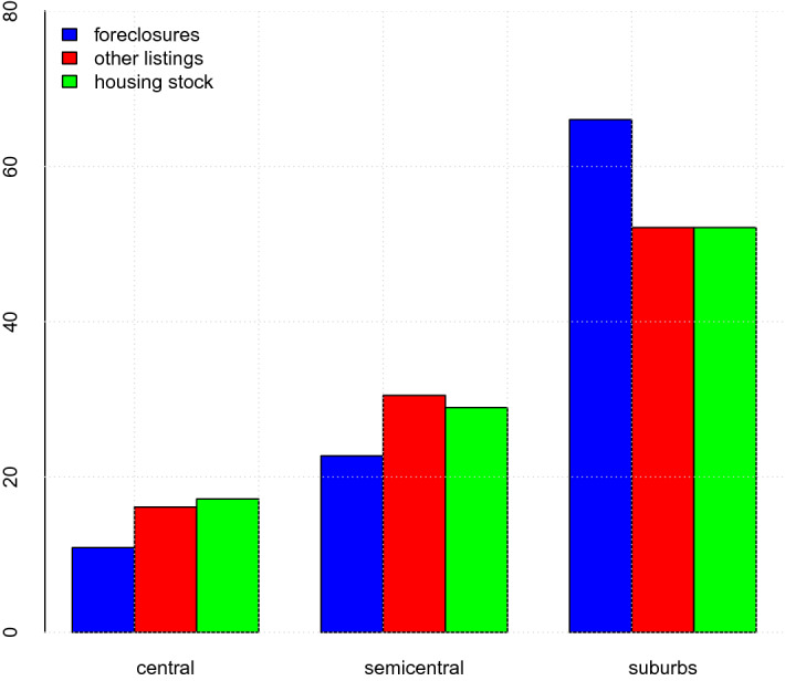
Distribution of foreclosed homes, other listings and housing stock inside by location (based on OMI classification). Percentage points. We merged the categories “suburbs” and “out-of-town”
We divide the territory of each city into local housing markets using the partition developed by OMI, a branch of the Italian Tax Office. The OMI microzones are contiguous areas of the city territory that satisfy strict requirements regarding the homogeneity of house prices, urban characteristics, socioeconomic characteristics, and the endowment of services and urban infrastructures. Unlike the census tracts, the OMI microzones are local homogeneous housing markets.13
The average number of households in an OMI microzone is 3,528 units, and the average housing stock is 4,166 units. The average share of owner-occupied households is 68.3%. The microzones have quite different sizes because they aim to approximate local housing markets. Table 6 in Appendix B reports the quantiles of the distributions of these variables and additional information about average house values and asking prices.
Table 6.
Descriptive statistics about the local markets
| Variable | Percentile | Mean | ||||
|---|---|---|---|---|---|---|
| 5 | 25 | 50 | 75 | 95 | ||
| Population | 270.2 | 1604.5 | 4473.0 | 10592.2 | 27589.3 | 8049.8 |
| Households | 108.6 | 681.8 | 1874.5 | 4582.2 | 12226.4 | 3528.5 |
| Housing units | 152.6 | 896.5 | 2388.0 | 5527.2 | 13750.6 | 4166.2 |
| Share of owner-occupied | 47.2 | 63.1 | 70.2 | 75.8 | 82.5 | 68.3 |
| Average house value | 765.6 | 1170.0 | 1532.5 | 2121.7 | 3339.0 | 1757.1 |
| Average asking price | 878.4 | 1290.1 | 1784.4 | 2453.8 | 4025.1 | 2013.5 |
Listing and Sale Prices
As we do not have access to administrative data on house sales, we observe only the listing prices. In general, this is a significant limitation, but it seems to be a less problematic issue in our case. In Fig. 2 we show that the average listing and sale prices in the cities of our sample have had a very similar evolution during the reference period we are considering.14 Listing prices declined slightly more than sale prices because of the simultaneous reduction in the average discount obtained by buyers.
Fig. 2.

Listing prices and sale prices. Indices 2017=100. a Reports aggregate indices for listing prices (Immobiliare.it) and sale prices (OMI) in all cities in our sample. b Reports listing and sale prices in the two main cities (Rome and Milan)
We are not claiming that considering listing prices is the same as observing sales prices. However, in the period covered by our analysis, it seems that listing prices are a good proxy for sale prices, and foreclosures are unrelated to the wedge between average listing and sale prices.
To confirm these hypotheses, we estimated the average discount on listing prices for all local housing markets based on listing prices and OMI data.15 In Italy, only a minimal share of transactions end up with a sale price equal to or higher than the listing price, and there is no evidence that owners set low asking prices to trigger an auction among potential buyers.16 In Fig. 3, we show that both the median and the weighted (by the housing stock) averages of the distribution of the discounts in the different microzones trend downward, albeit slightly. Considering the median of this distribution, the discount has been between 12 and 13% for 2017-2018. In the second half of 2016, the discount has been somewhat higher. This estimate is consistent with the Italian Housing Market Survey results, although the estimates of this survey refer to the whole country, not just to the cities in our sample (Fig. 3). In the following, we refer to the median as the best estimate for the discount, and during our reference period, it was 12.7% on average.
Fig. 3.

Discount applied to listing prices and time-on-market. a Reports the median and the weighted (using housing stocks) average for the discount across OMI microzones (measured in percentage points). The discount is computed as the ratio between the average listing price per s.m. and the average sale price per s.m. minus 1. b Reports the average discount (percentage points) and time-on market (months) in Italy according to the survey on real estate agents
Notice that in some cities the discount has been virtually stable. For example, in the two main Italian cities (Rome and Milan), the evolution of listing and sale prices in our reference period was almost the same (see Fig. 2).
On average, listing and sale prices have had the same evolution. However, there is still some concern that foreclosed homes may affect the average discount on the listing prices of non-foreclosed homes. If this is the case, we should find evidence of this relationship at the microzone level. We test for the presence of such a relationship using the following OLS model:
| 1 |
where is the ratio between the average listing and sale prices for non-foreclosed properties in microzone j, belonging to city k during the semester t. and are the number of foreclosed and non-foreclosed properties, respectively, listed during period t in the microzone j. and are city and time dummies, respectively. is a vector of microzone characteristics, namely the number of dwellings according to the 2011 Census and the location inside the city (central, semi-central, suburbs).
The results of this regression are reported in Table 8 in Appendix B. The coefficient for is not statistically significant, differently from the parameter . We find no correlation between the number of foreclosure listings and the average discount. On the opposite, a larger number of non-foreclosure listings increases the bargaining power of buyers and implies a larger wedge between listing and sale prices.
Table 8.
Determinants of the discount on listing prices
| Ratio between average listing and sale prices | |
|---|---|
| Foreclosures | −0.008 |
| (0.024) | |
| Other listings | 0.023 |
| (0.005) | |
| Housing stock | −0.001 |
| (0.000) | |
| Dummies | City + semester |
| Observations | 9,415 |
| Adjusted R | 0.270 |
The dependent variable is the ratio (multiplied by 100) between the average listing and sale prices in the local market i during the semester t. The regressors are the number of listings at time t. We control for the housing stock, the location inside the city, and we add city and time dummies. Significant at the 1% level. Significant at the 5% level. Significant at the 10% level
As a further argument to support the hypothesis that foreclosures do not affect the average discount on listing prices, in Sect. 6, we will show that there is no causal effect of foreclosures on the time-on-market in Italy. That is important because the correlation between time-on-market and average discount on asking prices is high. Therefore, it seems implausible that foreclosures affect the average discount but not the time-on-market. The positive correlation between the average discount and the time-on-market holds both at aggregate level (Fig. 3) and local housing market level (Table 8).17
Foreclosures Discount
According to the evidence of the previous section, foreclosed homes are sold at a price far lower than market values, in line with the results in the literature. On average, the reference prices of foreclosed houses are 52.4% points lower than the asking prices of other listings, partly because these houses may show up systematically different characteristics than those of other listings.
However, the literature has shown that foreclosed homes are traded at a lower price than market price even when different physical and location characteristics are considered. In this section, we want to estimate the percentage difference between the price of a foreclosed home and the price of houses sold in an unforced transaction, the so-called foreclosure discount. Unfortunately, we do not observe the sale prices. Then, we compare the last reference price established by the court to the listing prices for non-foreclosed properties. The estimate provides a valuable reference to identify the interval in which the discount on sale prices lies.
Following the methodology proposed in Campbell et al. (2011), we estimate the following regression model:
| 2 |
where is the logarithm of the last observed reference/asking price for dwelling i, located in the microzone j and delisted in quarter t. We control for house price variation over time at the microzone level by including the the terms . is the vector of physical characteristics of houses i, and includes the property type (apartment or detached house), size (square meters), number of bathrooms, presence of a balcony, parking space/box, maintenance status and floor level. Finally is a indicator variable that identifies if house i is sold through a judicial auction.
We also extend the baseline Eq. (2) to include an interaction term of with other house characteristics. In particular, we test if the discount varies with the house’s size, price, and geographical position inside the city. We also test if the discount depends on the tightness of the housing market at the city level, including the interaction term of with the year-on-year growth rate of house prices in the city.
Table 2 reports the estimates for the four different specifications. In the baseline regression (column 1), the estimate of is significant and equal to . That implies a price discount equal to percent.18 Columns 2 and 3 show that the foreclosure discount decreases with the size and the price of the house.
Table 2.
Foreclosure discount
| Listing price | |||||
|---|---|---|---|---|---|
| (1) | (2) | (3) | (4) | (5) | |
| Foreclosure | −0.653 | −0.811 | −0.857 | −0.667 | −0.486 |
| (0.003) | (0.005) | (0.004) | (0.004) | (0.010) | |
| Foreclosure Floor area | 0.002 | ||||
| (0.000) | |||||
| Foreclosure Price | 0.000 | ||||
| (0.000) | |||||
| Foreclosure Market tightness | −0.008 | ||||
| (0.001) | |||||
| Foreclosure Location: semi-central | −0.111 | ||||
| (0.012) | |||||
| Foreclosure Location: suburbs | −0.233 | ||||
| (0.011) | |||||
| Foreclosure Location: out-of-town | −0.185 | ||||
| (0.030) | |||||
| Dummies | Microzone | Microzone | Microzone | Microzone | Microzone |
| -quarter | -quarter | -quarter | -quarter | -quarter | |
| Observations | 550,219 | 550,219 | 550,219 | 543,816 | 543,984 |
| Adjusted R | 0.536 | 0.537 | 0.542 | 0.527 | 0.536 |
The dependent variable is the log of the last observed asking price before delisting. We control for the following home physical characteristics: property type (apartment or detached house), size (square meters), number of bathrooms, presence of a balcony, parking space/box, maintenance status and floor level. Time effects refer to the quarter in which a house is delisted. Significant at the 1% level. Significant at the 5% level. Significant at the 10% level
In column 4, we test if the discount is affected by the tightness of the housing market, using as a proxy of market tightness the year-on-year growth rate of asking prices of non-foreclosure listings. We compute these growth rates at the city level instead of at the local market level to avoid potential spillovers from foreclosed properties to the asking prices of the other listings. The hypothesis is that the foreclosure discount is lower in cities the housing market is performing better. However, we find that the interaction term is statistically significant but very small. Then, there is no relevant systematic difference in the foreclosure discount between cities where prices increase and those where they are falling.
Finally, column 5 reports that the magnitude of the price discount is strongly affected by the geographical position inside the city. For houses in the city center, the price discount is roughly 38 percent and increases moving outward. The price discount of foreclosed homes in suburbs is higher than 50%.
Estimation of the Sale Price Discount
As we have already said, we do not observe sale prices. For foreclosed houses, we know the reference price set by the court. For the other homes, we observe the asking prices posted by the sellers. In this section, we use our estimates based on listing prices and additional data sources to estimate the percentage difference between the sale price of a foreclosed home and the sale price of houses sold in unforced transactions. Although we cannot provide a point estimate of the foreclosure sale price discount, we can identify a reasonable interval for this parameter.
Regarding the sale price of foreclosed homes, the institutional details of judicial auctions allow us to make reasonable assumptions about the interval in which the final price for foreclosed properties is. The court sets the reference price, starting from the estimated market value of the house. If there are no bids, the court decreases the reference price up to 25% and calls for new bids. That goes on iteratively as long as no bid is made. Since the minimum bid in each round can be computed by discounting the reference price set by the court by 25%, the last reference price is plausibly an upper bound for the sale price of the foreclosed home, while the minimum offer is a lower bound.
Then, we also use our preferred estimate of the average discount applied to the asking prices, which is 12.7% (see Sect. 3.1), to discount listing prices.
Under these assumptions, the average foreclosure discount to sale prices is approximately between 42 and 56%,19 a range that is consistent with the estimates of market operators.20 These figures are much higher compared to the evidence for the US.21 A possible explanation for this result is that the market for foreclosed homes is isolated from the other segments of the housing market.22 If this is the case, we should expect limited spillovers from foreclosures to the housing market. We investigate this hypothesis in the next section.
The Competitive Effect of Foreclosures
In this section, we evaluate the impact of a foreclosed property’s entry on the probability of observing price revisions for nearby non-foreclosed homes. In this way, we test if the presence of foreclosed homes affects home sellers’ strategies in the housing market. The hypothesis is that foreclosures compete with other dwellings because their price is much lower than the market value. If this is the case, some home sellers may decide to revise downward their listing price. Therefore, we cannot consider the market for foreclosed homes isolated from the other housing market segments, notwithstanding the high foreclosure discount would point to a very limited arbitrage between housing market segments.
We implement the identification scheme proposed by Anenberg and Kung (2014). We test if a price revision is more likely to happen in the few weeks following the listing of a new nearby foreclosed home. This identification strategy relies on the assumption that the listing timing of a foreclosed home is not correlated with any local shock that may cause sellers to adjust their list prices. This assumption is reasonable because strategic concerns do not motivate the entry of a foreclosed home into the market, which is the output of an administrative process and is mostly determined by exogenous factors.
As noticed by Anenberg and Kung (2014), observing a price revision around the market entry of a foreclosed home is evidence that foreclosed properties compete with other listings. Therefore, the market for foreclosed houses would be linked to the other segments of the housing market.
Notice that this is only one possible channel through which foreclosures affect the housing market. In particular, foreclosures may negatively affect the microzone to which they belong because of the so-called disamenity effect. Foreclosures involve periods during which houses stand empty, and they lack maintenance expenditures. That may reduce the neighborhood’s appeal, and an increasing concentration of empty houses may eventually encourage crime. However, the effects of these disamenities should take place well before the listing of the foreclosed home, and it should start at the time of the foreclosure. If we observe an effect around the listing week, it is more plausible that competitive forces are at work.
We estimate how the probability of a price revision is affected by foreclosures entry using the following linear probability model:
| 3 |
where it is an indicator variable equal to 1 if house i, belonging to microzone j, changes its listing price downward in week t. () is the logarithm of one plus the number of new foreclosures (other listings) entering into the market in week that are within a radius r of listing i.23 We consider both lags and leads to check that home sellers do not know in advance about the exact week of listing of a foreclosed home. As in Anenberg and Kung (2014) we consider the logs because in standard price competition models the competitive effect should be concave in the number of competitors. is a set of week-by-microzone fixed effects. is a vector of controls, which includes an indicator for whether the listing is a foreclosure, the number of days that the home has been on the market, the floor area of the house, and the type of property.
We estimate Eq. (3) over the full sample for three different values of the radius r: 150, 300 and 450 m. We report the most relevant parameters in Table 3 while the full results of the three specifications can be found in Table 9 in Appendix B. We consider different specifications for the distance because there is ample evidence in the literature that the foreclosure impact is stronger for closer non-foreclosed homes. We want to test if the effect of foreclosures fades out over longer distances and then becomes no longer significant.
Table 3.
Determinants of price changes
| Price change | |||
|---|---|---|---|
| (1) | (2) | (3) | |
| New foreclosures t-1 | 0.0031 | 0.0011 | 0.0005 |
| (0.0004) | (0.0002) | (0.0002) | |
| New foreclosures t | 0.0019 | 0.0008 | 0.0005 |
| (0.0004) | (0.0002) | (0.0002) | |
| New (no forecl.) listings t-1 | 0.0005 | 0.0004 | 0.0003 |
| (0.0001) | (0.0001) | (0.0001) | |
| New (no forecl.) listings t | 0.0001 | 0.0001 | 0.0000 |
| (0.0001) | (0.0001) | (0.0001) | |
| Dummies | Microzone-week | Microzone-week | Microzone-week |
| Observations | 14,765,969 | 14,765,969 | 14,765,969 |
| Adjusted R | 0.0029 | 0.0029 | 0.0029 |
We report only the most relevant parameters (see Table 9 for the other parameters). The dependent variable is an indicator variable taking value equal to 1 if the owner of house i revises the listing price in week t. The number of new nearby listings that are within a radius r of listing i is measured in logs. We consider three different values for r: 150 m (column 1), 300 m (column 2), 450 m (column 3). We control for the type of property, its size, its time on market up to week t and a dummy variable that identify if it is a foreclosure listing. All changes are relative to a baseline probability of adjusting list price of 0.014. Significant at the 1% level. Significant at the 5% level. Significant at the 10% level
Table 9.
Determinants of price changes
| Price change | |||
|---|---|---|---|
| (1) | (2) | (3) | |
| New foreclosures t-4 | −0.0009 | −0.0001 | 0.0001 |
| (0.0004) | (0.0002) | (0.0002) | |
| New foreclosures t-3 | −0.0004 | −0.0001 | −0.0002 |
| (0.0004) | (0.0002) | (0.0002) | |
| New foreclosures t-2 | −0.0001 | −0.0001 | 0.0002 |
| (0.0004) | (0.0002) | (0.0002) | |
| New foreclosures t-1 | 0.0031 | 0.0011 | 0.0005 |
| (0.0004) | (0.0002) | (0.0002) | |
| New foreclosures t | 0.0019 | 0.0008 | 0.0005 |
| (0.0004) | (0.0002) | (0.0002) | |
| New foreclosures t+1 | −0.0001 | 0.0001 | −0.0001 |
| (0.0004) | (0.0002) | (0.0002) | |
| New foreclosures t+2 | 0.0000 | −0.0001 | −0.0002 |
| (0.0004) | (0.0002) | (0.0002) | |
| New foreclosures t+3 | −0.0004 | −0.0001 | −0.0000 |
| (0.0004) | (0.0002) | (0.0002) | |
| New foreclosures t+4 | 0.0006 | 0.0007 | 0.0004 |
| (0.0004) | (0.0002) | (0.0002) | |
| New (no forecl.) listings t-4 | −0.0000 | 0.0000 | 0.0001 |
| (0.0001) | (0.0001) | (0.0001) | |
| New (no forecl.) listings t-3 | −0.0002 | −0.0000 | −0.0001 |
| (0.0001) | (0.0001) | (0.0001) | |
| New (no forecl.) listings t-2 | −0.0001 | −0.0001 | 0.0001 |
| (0.0001) | (0.0001) | (0.0001) | |
| New (no forecl.) listings t-1 | 0.0005 | 0.0004 | 0.0003 |
| (0.0001) | (0.0001) | (0.0001) | |
| New (no forecl.) listings t | 0.0001 | 0.0001 | 0.0000 |
| (0.0001) | (0.0001) | (0.0001) | |
| New (no forecl.) listings t+1 | −0.0001 | 0.0000 | 0.0001 |
| (0.0001) | (0.0001) | (0.0001) | |
| New (no forecl.) listings t+2 | −0.0003 | −0.0001 | 0.0000 |
| (0.0001) | (0.0001) | (0.0001) | |
| New (no forecl.) listings t+3 | 0.0001 | 0.0003 | 0.0002 |
| (0.0001) | (0.0001) | (0.0001) | |
| New (no forecl.) listings t+4 | −0.0005 | −0.0002 | −0.0002 |
| (0.0001) | (0.0001) | (0.0001) | |
| Dummies | Microzone-week | Microzone-week | Microzone-week |
| Observations | 12,342,092 | 12,342,092 | 12,342,092 |
| Adjusted R | 0.0028 | 0.0028 | 0.0028 |
The dependent variable is an indicator variable taking value equal to 1 if the owner of house i revises the listing price in week t. The number of new nearby listings that are within a radius r of listing i is measured in logs. We consider three different values for r: 150 m (column 1), 300 m (column 2), 450 m (column 3). We control for the type of property, its size, its time on market up to week t and a dummy variable that identify if it is a foreclosure listing. All changes are relative to a baseline probability of adjusting list price of 0.014. Significant at the 1% level. Significant at the 5% level. Significant at the 10% level
The effect of a new foreclosure listing in a radius of 150 m is both statistically significant and economically relevant (Column 1). Considering both the parameters associated with and , the additional probability of a price change caused by a new nearby foreclosure listing (relative to null) is 0.3 percent.24 This is a sizeable effect because home sellers do not frequently adjust their asking price in Italy: the average probability of adjusting the list price is 1.4%. Indeed, Anenberg and Kung (2014) finds that in San Francisco, the effect of new foreclosure listing on the propensity of home sellers to change their price is more than twice our estimate. However, we must compare this additional probability against a much higher baseline probability of price adjustment, about 7% in San Francisco.
The market entry of a non-foreclosure listing also has a statistically significant impact on the propensity to revise listing prices. However, the additional probability of changing the price is less than 0.1% points.25 We observe a smaller reaction than the listing of foreclosed properties plausibly because the latter enter the market with relatively low prices.
Columns 2 and 3 report the results of regression (3) when the radius r is 300 and 450 m, respectively. We find that spillovers from foreclosures are very local and dies out quite fast as the distance increases. The effect of foreclosures on the propensity to change the list price is more than halved at a distance of 300 m and is very small when the radius is 450 m.
The effect of foreclosures on non-foreclosed house prices
Since sellers react to the market entry of foreclosures, we cannot consider the market for foreclosed houses isolated from other segments of the real estate market, even if the spillovers are local. Consequently, it is essential to investigate the extent to which foreclosures influence the prices of nearby non-foreclosed houses.
The estimation of this effect is a complex task because of the strong interrelationship between foreclosures and house prices. First, we discussed in Sect. 4 that foreclosures are mainly in peripheral and suburban areas. Then, it is hard to say that they are random. Second, foreclosures are endogenous to house prices because a fall in house prices reduces dwellings’ equity value. Suppose the value of a house falls below that of the outstanding mortgage debt taken to buy it (negative equity). In that case, the homeowner has the incentive to default on his debt strategically. In principle, this is a mild issue in Italy because mortgage loans to households are recourse, but there is some concern about the behavior of companies.26 Third, there can be common shocks that may affect both house prices and foreclosures. A typical example is an income shock resulting from the shutdown of some relevant economic activity within the neighborhood. Some debtors may lose their jobs and no longer be able to pay their debts. Their homes would be foreclosed and sold through judicial auctions. At the same time, a lower income in the neighborhood would lead to lower demand for housing and thus lower house prices.
Mian et al. (2015) identify the causal impact of foreclosures on house prices using an instrumental variable approach. They find that the procedure to sell the collateral adopted in the different US States—judicial or nonjudicial foreclosures—affects the propensity of a house to be foreclosed but does not influence house prices except through foreclosures. As we cannot employ a similar identification strategy for the Italian case, we follow a variation of the approach proposed by Campbell et al. (2011) and Anenberg and Kung (2014).
To control for endogeneity, we compare the effect on the last asking price of a non-foreclosed home of nearby foreclosure listings before and after its delisting. We know the number of nearby foreclosure listings in the weeks before and after the delisting of a house. To the extent that foreclosures negatively affect house prices, we expect the coefficient associated with the number of foreclosure listings before the delisting to have a larger magnitude.
At the same time, to control for common economic shocks, we distinguish foreclosure listings in an inner circle with a radius of 150 m and those in an outer ring with a distance in the interval 150–400 m for each delisted house. The listings in the outer ring can be considered a control group. A common negative shock should generate the same downward trend in house prices over a 400 m distance, absent any foreclosure. Moreover, since foreclosure spillovers are local, they should be stronger on the prices of closer houses. The results in the previous section indicate that this is a reasonable assumption, and they provide support for the choice of the radius.27
To interpret our results in terms of spillovers on sale prices, it must be the case that the listing of a foreclosed home: (i) does not affect the average discount applied to the listing prices of nearby homes, and (ii) does not change the probability that delisting of a nearby home corresponds to a sale instead of a withdrawal. The analysis in Sect. 3.1 provides evidence that the first condition is satisfied. Moreover, the evidence that home sellers revise their listing price following the listing of a nearby foreclosed property further enhances the results in Sect. 3.1.
Regarding the second condition, instead, the listing of a nearby foreclosed property could lead to a higher incidence of withdrawals. Therefore, listing prices would be a poor proxy for sale prices precisely where more foreclosed properties are listed.28 However, the opposite could also be true. Home sellers may want to speed up the sale of their house because they expect that the listings of foreclosed properties can induce a reduction in house prices. We do not have microdata to test if condition (ii) is satisfied. However, since there is no causal impact of foreclosures on the time-on-market—as we will show below—and there is no correlation of foreclosure listings with the average discount on listing prices is reassuring evidence.
We enrich regression (2) by including measures of nearby foreclosures as covariates. Let () denote the log count of foreclosures listings within a 150 m radius of dwelling i during the 60 days before (after) the delisting of dwelling i.29 and are similarly defined, but we consider listings between 150 and 400 m.30 We estimate the following regression:
| 4 |
where is the logarithm of the last observed listing price for a non-foreclosed dwelling i, located in the microzone j and delisted in month t. As in Sect. 4 we control for house price variation over time at the microzone level and for the physical characteristics of houses i. Finally, we control for the log of the number of non foreclosure listings, as for foreclosures. That allows us to estimate if the effect of foreclosures is similar to the one of any other listing.
This specification is different from 3 because we are interested in the effect on house prices of a nearby foreclosure listing—i.e., the fact that it is on the market for several weeks and compete with other houses—not just its market entry.31
We measure the spillover effect of foreclosures on nearby house prices as , namely the difference between past and future foreclosure coefficients in the inner ring, controlling for past and future foreclosures within the outer ring. Similarly, we compute the spillover effect of other listings as . We also estimate a more parsimonious version of (4), in which we consider only the information about the past listings.
Table 4 reports our results. In Column 1, we show the estimates of the reduced model. Since we are considering a log-log model, the impact on the asking price of having one nearby foreclosure listing (relative to none) in the 60 days before delisting is -3.6%.32 The impact of having a non-foreclosure listing is still negative, but much smaller .
Table 4.
Local effects of foreclosures on house prices and time-on-market
| Listing price | Time on market | Listing price | Time on market | |
|---|---|---|---|---|
| (1) | (2) | (3) | (4) | |
| 0.0057 | −0.0029 | |||
| (0.0012) | (0.0030) | |||
| −0.0178 | 0.0060 | |||
| (0.0012) | (0.0030) | |||
| −0.0114 | 0.0300 | |||
| (0.0010) | (0.0026) | |||
| −0.0519 | −0.0077 | |||
| (0.0015) | (0.0039) | |||
| −0.0002 | 0.0091 | |||
| (0.0058) | (0.0148) | |||
| −0.0021 | −0.0070 | |||
| (0.0035) | (0.0090) | |||
| −0.0158 | 0.0436 | |||
| (0.0049) | (0.0126) | |||
| −0.0162 | 0.0060 | |||
| (0.0047) | (0.0119) | |||
| Dummies | Microzone-month | Microzone-month | Microzone-month | Microzone-month |
| Observations | 407,167 | 407,177 | 407,167 | 407,177 |
| Adjusted R | 0.5219 | 0.0137 | 0.5220 | 0.0137 |
The dependent variables and the number of nearby listings are measured in logs. Parameters denoted by are associated with nearby foreclosures listings, while refers to other listings. We control for the following home physical characteristics: property type (apartment or detached house), size (square meters), number of bathrooms, presence of a balcony, parking space/box, maintenance status and floor level. Time effects refer to the month in which a house is delisted. Significant at the 1% level. Significant at the 5% level. Significant at the 10% level
According to this specification, also foreclosures in the outer ring affect house prices. However, their spillovers, as measured by , are much lower than those nearby. That is consistent with our identification strategy and with the estimates of the previous section.
We report the results of our full specification in Column 3. The impact of a foreclosure on house prices in the inner circle (relative to the outer ring) is This is an estimate consistent with those of Campbell et al. (2011) and Anenberg and Kung (2014) for the US. According to Campbell et al. (2011), a foreclosure that takes place 0.05 miles away—that is about half the distance we consider in this study—lowers the price of a nearby house by about 1%.33 Instead, for Anenberg and Kung (2014) houses that are less than 0.1 miles from a foreclosure listing are sold at a 1.6% lower price. Also, the effect of foreclosures is the same as other listings, as in Anenberg and Kung (2014). The effect of listings in the outer circle is negative, although not statistically significant for foreclosures and other listings.
To understand the implications of foreclosures for market liquidity, we considered an additional specification in which the dependent variable is the logarithm of the number of days the dwelling has been listed. Columns 2 and 4 report the results. The number of non-foreclosure listings has a significant impact on time-on-market. One listing in the inner circle (compared to none) implies that the time-on-market is higher by 3.2%. On the opposite, foreclosures do not affect the time-on-market.
Conclusion
We investigate the impact of foreclosures on the Italian housing market. Despite a considerable foreclosure discount suggests that the market for foreclosures is isolated from other housing market segments, we find evidence of significant spillovers from foreclosures to the market of non-foreclosed homes.
Home sellers have a higher propensity to revise downward their asking price in the same week and the week following the market entry of a nearby foreclosure. This effect is local and decreasing in the distance from the foreclosed house.
Foreclosures compete in the housing market with non-foreclosure listings and affect the prices of nearby non-foreclosed houses. We find that the impact of foreclosures on nearby house prices is negative and significant.
In recent years, the number of foreclosures has been very high compared to the period preceding the global financial crisis compared with the total number of transactions in the housing market. Our econometric strategy does not quantify the effect of foreclosures on the aggregate trend of house prices in Italy. However, our results suggest that foreclosures are likely to be one of the factors that have dampened house prices in Italy in the last decade.
Moreover, understanding the impact of foreclosures on housing prices is essential to assess the outlook for the Italian housing market. The economic recession caused by the COVID-19 epidemic may lead to a new wave of mortgage defaults and foreclosures. The significant foreclosure discount suggests the need to make selling foreclosed properties even more effective to increase the recovery rate of bank non-performing loans. Furthermore, we now know that foreclosures affect housing prices. Therefore, a large increase in foreclosure could harm housing market performance in the coming years.
Data
Listings. The source data which we obtained from Immobiliare.it are contained in weekly files.
The information available for each ad is reported in Table 5.
Table 5.
Information contained in the database provided by Immobiliare.it.
| Type of data | Variables |
|---|---|
| Numerical | Price, floor area, rooms, bathrooms |
| Categorical | Property type, furniture, kitchen type, heating type, maintenance status, balcony, terrace, floor, air conditioning, energy class, basement, utility room |
| Related to the building | Elevator, type of garden, garage, porter, building category |
| Contractual | Foreclosure auction, contract type |
| Related to the seller | Publisher type (private citizen or real estate agency), agency name and address |
| Geographical | Longitude, latitude, address |
| Temporal | Ad posted, ad removed, ad modified |
| Textual | Description |
For a complete description of the meaning of the variables, see Loberto et al. (2020). If the variables in italic are missing, we perform semantic analysis on the textual description of the ads to recover the information
House prices. OMI, a branch of the Italian Tax Office, disseminates estimates of the minimum and maximal house values in euros per square meter, and , at a very granular level twice per year. House values are available for all types of properties (i.e., apartments or detached houses) and OMI zones – which are uniform socio-economic areas – in the Italian cities. OMI design these microzones in order to have a set of homogeneous local housing markets. and are estimated based on a limited sample of house sales and valuations by real estate experts. Further information is available at https://www.agenziaentrate.gov.it/wps/content/Nsilib/Nsi/Schede/FabbricatiTerreni/omi.
Multiple estimates for house prices can exist for a microzone, one for each type of property prevalent in the microzone. Unfortunately, the classification of property types follows the cadastral registry, which is not very precise. Moreover, we do not know the composition of the housing stock in each microzone, and therefore we cannot compute the correct weights to aggregate the different estimates.
We define the average house value in the OMI microzone j as , where is the number of property types in microzone j. and are the minimum and maximum price, respectively, for each house typology.
We estimate the average house values at the city level as a simple average of the . For further aggregation, we compute weighted averages of the cities’ average house values. We use as weights the stock of houses according to the 2011 Census. OMI estimates are not designed for statistical purposes, and the index we construct must not be considered equivalent to a quality-adjusted price index.
Istat disseminates quality-adjusted (hedonic) house price indexes. However, their indicators’ reference area is not consistent with our listing data, apart from three city-level indexes referred to the main Italian cities: Rome, Milan and Turin.
Census data. We retrieve detailed information on the neighborhood’s socio-economic characteristics and the stock of buildings in the surrounding area from the 2011 Census. Istat census tracts are much smaller than OMI micro-zones (indeed, there are approximately 400,000 Istat census tracts over the Italian territory compared to 27,000 OMI micro-zones) and do not necessarily coincide with them. We perform spatial matching of the polygons representing the tracts and the micro-zones and impute the Istat variables to the OMI micro-zones according to the overlap percentage of the polygons. For example, if an Istat census tract comprises 2,000 housing units and it straddles two OMI micro-zones, such that there is a 50% overlap for both, we impute 1,000 housing units to each of the two OMI micro-zones.
Italian Housing Market Survey. The Italian Housing Market Survey, conducted quarterly by Banca d’Italia, Tecnoborsa and OMI, covers about 1,200 real estate agents and describes their opinions regarding the current and expected course of house sales, price trends, rental prices and contracts. This paper considers the survey results about the average discount on listing prices and the time-on-market.
The average discount is computed based on the answers to the following question: For the primary property type sold in the reference quarter, compared with the seller’s first asking price, how was the selling price? Real estate agents must reports an interval for the discount (higher than 30%, between 20% and 30%, between 10% and 20%, between 5% and 10%, less than 5%, selling price equal (or higher than) the asking price). The average discount is computed as the weighted average of the mean values in each interval.
The estimate of the time-on-market is based on the following question: Considering the total number of homes sold by you in the reference quarter, how many months passed on average between a house being registered with you and its sale (signature of preliminary contract)? Agents reply to this question by reporting the number of months. Then, the final statistics are computed by averaging the values reported by the agents.
Additional informations is available at https://www.bancaditalia.it/pubblicazioni/sondaggio-abitazioni/index.html?com.dotmarketing.htmlpage.language=1.
Estimation of the discount on listing prices. We computed for each microzone j and semester t the ratio between the average listing price per s.m., , and the average house prices per s.m. based on OMI data, . The latter are estimated based on the procedure described above. Then, we compute the discount as .
There is a critical measurement issue. For many microzones, OMI disseminates multiple estimates—one per property typology—and we do not know the composition of the housing stock for each microzone. Therefore, can be a biased estimate of the average house prices in microzone j. Consequently, the average discount may be biased for some microzone and even unreliable in some cases.
However, we find that the median of the distribution of the average discount across microzones (12.7%) is consistent with the results of the Italian Housing Market Survey, where real estate agents provide an estimate based on the transaction they brokered (see Fig. 3).34 Moreover, the bias is constant over time, as the composition of the housing stock is almost fixed in the short period that we consider. Different property typologies show off minimal heterogeneity in the growth rates of their prices inside a microzone.
Additional tables
Table 10.
Time-on-market and average discount to listing prices
| Ratio between average listing and sale prices | |
|---|---|
| Time-on-market | 0.020 |
| (0.010) | |
| Housing stock | −0.000 |
| (0.000) | |
| Observations | 1,880 |
| Adjusted R | 0.307 |
The dependent variable is the ratio (multiplied by 100) between the average listing and sale prices in the local market i in the whole period. The time-on-market is measured in days. We control for the housing stock, the location inside the city, and we add city dummies. Significant at the 1% level. Significant at the 5% level. Significant at the 10% level
Figures
Footnotes
During the period 2016–2018, the average annual number of property sales was about 1.1 million.
Since the beginning of the epidemic, the government has taken several measures to prevent a sharp increase in foreclosures. However, these measures are temporary. In the absence of their renewal, foreclosures may begin to increase.
Until 2015, for example, the buyer of a foreclosed home had to pay the price offered in a single installment, and he could not take out a mortgage for the purchase.
When the loan is recourse, the lender can go after all the borrower’s assets until he gets a full repayment of the loan.
Following the market entry of a foreclosure, the probability of changing the list price increases by 0.3% points. This effect is sizeable because home sellers do not frequently adjust their asking price in Italy. The average probability of changing the list price is 1.4%.
This issue is in Italy less relevant than in the US because mortgage loans to households are recourse.
Following three unsuccessful auctions, the reference price can be reduced up to 50%.
According to Astasy, 78% of the judicial sales that took place in 2017 were related to foreclosures, while the remainder were associated with companies’ bankruptcy proceedings. Since companies in Italy hold only about 7% of the housing stock, it is reasonable to assume that judicial auctions are associated with foreclosures.
The main innovation of the subsequent 2016 reform was the introduction of the power of law clause (Patto Marciano). The new law makes it possible to include in the mortgage loan agreements a specific provision that allows the bank the right to obtain ownership of the house through an out-of-court proceeding following the default of the debtor. According to Bank of Italy (2018), this clause has not been used by Italian banks until 2018. Moreover, since it would apply only to new contracts, it is implausible that foreclosures following this alternative procedure already occurred.
For a more detailed description of the regulatory framework, see Giacomelli et al. (2019) and the references therein.
Nomenclature of Territorial Units for Statistics (NUTS) is the geocode used in Europe for referencing the subdivisions of countries for statistical purposes.
We explain below our definition of the local housing market.
OMI microzones are periodically revised to satisfy these criteria and to better approximate local housing markets. The last revision dates back to 2014.
See Appendix A for the details about sale prices.
See Appendix 3 for a description of the methodology that we used to estimate the discount.
According to the Italian Housing Market Survey, in our reference period, that share was about 5%. In general, brokers do not accept other offers if the seller is already negotiating with a potential buyer, ruling out auctions for the same house.
In Table 8, we report the results of the regression of the average ratio between listing and sale prices for non-foreclosed properties during the reference period and the average time-on-market. We control for city effects and the microzone characteristics considered in (1). As expected, a longer time-on-market is associated with a larger wedge between listing and sale prices.
Kennedy (1981) shows that the OLS estimate of in (2) is biased, and the distortion can be corrected by taking into account the square of the standard error of the estimated parameter. Since the standard error is tiny (0.003), this correction would not change the estimated foreclosure discount.
We obtain the lower bound of the interval by multiplying the estimate of the previous section, 48.0%, by to keep into account the discount on asking prices. When we estimate the lower bound, we assume that the sale price of a foreclosed property is equal to the court’s reference price. To compute the upper bound, instead, we must consider that the selling price of a foreclosed property can be up to 25% lower than the benchmark price set by the court.
According to Astasy, the average discount was 55% in 2017. However, they did not disclose the methodology behind their estimate, and we cannot compare their estimate with ours.
Campbell et al. (2011) find that the foreclosure discount is 27% on average, while for Anenberg and Kung (2014) the estimate is 16%. Cohen et al. (2016) show that the estimates of the foreclosure discount in the US range between 0 and 28%.
Recent reforms have made it easier for potential buyers to access this market. However, buyers may be either unaware of the regulatory changes or consider this market still too opaque. Alternatively, brokerage and legal costs may still be too high.
Since we take the log count of listings, we add one to avoid computing the logarithm of zero.
This estimate can be retrieved by multiplying the parameters in Table 3 by . Given the linear-log specification of the model, we are computing the effect of one new listing, , compared to none, .
Other estimated parameters are statistically significant, but we do not comment on them because they are not economically meaningful.
The lender can go after other family assets if the value of the house is not enough to cover the debt. However, in practice, a significant share of the foreclosed dwellings may originate from companies’ defaults, notably from construction firms. Companies continue to have the incentive to default because of limited liability.
The distances that we consider are very similar to those used in the literature for the US.
The listing prices of withdrawn properties may be systematically different from those of houses transacted. In particular, the listing prices of withdrawn houses are likely higher than those sold. For this reason, we would be underestimating the negative spillover of foreclosures on house prices.
Also in this case, we add one to avoid computing the logarithm of zero.
The choice to consider the logarithm of the number of foreclosures is motivated by the results of (Campbell et al. 2011). They find that the effect of nearby foreclosures is concave in the number of foreclosures.
Our specification is very similar to Campbell et al. (2011) and Anenberg and Kung (2014). Differently from us, Campbell et al. (2011) consider a one-year time window for foreclosures before and after the sale of a house, and they do not control for the listing of non-foreclosed properties. Anenberg and Kung (2014) use sale prices as the dependent variable and consider a richer specification, where they control for the number of foreclosed and not-foreclosed properties in all their different stages of the listing process.
The effect of an additional foreclosure listing relative to none is .
Hartley (2014) has found a similar result.
The results of the survey on real estate agents refer to the whole country, not just to the cities in our sample.
The views expressed in this article are those of the author and do not reflect the views of Banca d’Italia.
Publisher's Note
Springer Nature remains neutral with regard to jurisdictional claims in published maps and institutional affiliations.
References
- Anenberg E, Kung E. Estimates of the size and source of price declines due to nearby foreclosures. Am Econ Rev. 2014;104(8):2527–51. doi: 10.1257/aer.104.8.2527. [DOI] [Google Scholar]
- Bank of Italy, Annual Report (2018)
- Calomiris Charles W, Longhofer Stanley D, Miles William R (2013) The foreclosure–house price nexus: a panel VAR model for US states, 1981–2009. Real Estate Econ 41(4):709–746
- Campbell JY, Giglio S, Pathak P. Forced sales and house prices. Am Econ Rev. 2011;101(5):2108–31. doi: 10.1257/aer.101.5.2108. [DOI] [Google Scholar]
- Ciocchetta F, Cornacchia W, Felici R, Loberto M (2016) Assessing financial stability risks from the real estate market in Italy. Questioni di Economia e Finanza (Occasional Papers) 323. Bank of Italy, Economic Research and International Relations Area March
- Cohen Jeffrey P, Coughlin Cletus C, Yao Vincent W (2016) Sales of distressed residential property: what have we learned from recent research? Federal Reserve Bank of St. Louis Rev 3:159–88
- Fisher LM, Lambie-Hanson L, Willen P. The role of proximity in foreclosure externalities: evidence from condominiums. Am Econ J Econ Policy. 2015;7(1):119–40. doi: 10.1257/pol.20130102. [DOI] [Google Scholar]
- Foote CL, Gerardi K, Willen PS. Negative equity and foreclosure: theory and evidence. J Urban Econ. 2008;64(2):234–245. doi: 10.1016/j.jue.2008.07.006. [DOI] [Google Scholar]
- Gerardi K, Eric R, Paul SW, Vincent Y (2015) Foreclosure externalities: new evidence. J Urban Econ 87:42–56
- Giacomelli S, Orlando T, Rodano G (2019) Real estate foreclosures: the effects of the 2015-16 reforms on the length of the proceedings. Notes on Financial Stability and Supervision 16, Bank of Italy
- Guren AM, Timothy JM (2019) How do foreclosures exacerbate housing downturns?. National Bureau of Economic Research, Technical Report
- Harding JP, Rosenblatt E, Yao VW. The contagion effect of foreclosed properties. J Urban Econ. 2009;66(3):164–178. doi: 10.1016/j.jue.2009.07.003. [DOI] [Google Scholar]
- Harding JP, Rosenblatt E, Yao VW (2012) The foreclosure discount: Myth or reality?. J Urban Econ 71(2):204–218
- Hartley D. The effect of foreclosures on nearby housing prices: supply or dis-amenity? Regional Sci Urban Econ. 2014;49:108–117. doi: 10.1016/j.regsciurbeco.2014.09.001. [DOI] [Google Scholar]
- Immergluck D, Smith G. The external costs of foreclosure: the impact of single-family mortgage foreclosures on property values. House Policy Debate. 2006;17(1):57–79. doi: 10.1080/10511482.2006.9521561. [DOI] [Google Scholar]
- Kennedy PE. Estimation with correctly interpreted dummy variables in semilogarithmic equations. Am Econ Rev. 1981;71(4):801. [Google Scholar]
- Lambie-Hanson L. When does delinquency result in neglect? Mortgage distress and property maintenance. J Urban Econ. 2015;90:1–16. doi: 10.1016/j.jue.2015.07.002. [DOI] [Google Scholar]
- Loberto M, Luciani A, Pangallo M (2020) What do online listings tell us about the housing market?
- Mian A, Sufi A, Trebbi F. Foreclosures, house prices, and the real economy. J Financ. 2015;70(6):2587–2634. doi: 10.1111/jofi.12310. [DOI] [Google Scholar]
- Osservatorio del Mercato Immobiliare (2017) Manuale della Banca Dati Quotazioni dell’Osservatorio del Mercato Immobiliare
- Towe C, Lawley C. The contagion effect of neighboring foreclosures. Am Econ J Econ Policy. 2013;5(2):313–35. doi: 10.1257/pol.5.2.313. [DOI] [Google Scholar]