Bifurcation analysis of a discrete-time compartmental model for hypertensive or diabetic patients exposed to COVID-19

Abstract

In this article, a mathematical model for hypertensive or diabetic patients open to COVID-19 is considered along with a set of first-order nonlinear differential equations. Moreover, the method of piecewise arguments is used to discretize the continuous system. The mathematical system is said to reveal six equilibria, namely, extinction equilibrium, boundary equilibrium, quarantined-free equilibrium, exposure-free equilibrium, endemic equilibrium, and the equilibrium free from susceptible population. Local stability conditions are developed for our discrete-time mathematical system about each of its equilibrium point. The existence of period-doubling bifurcation and chaos is studied in the absence of isolated population. It is shown that our system will become unstable and experiences the chaos when the quarantined compartment is empty, which is true in biological meanings. The existence of Neimark–Sacker bifurcation is studied for the endemic equilibrium point. Moreover, it is shown numerically that our discrete-time mathematical system experiences the period-doubling bifurcation about its endemic equilibrium. To control the period-doubling bifurcation, Neimark–Sacker bifurcation, a generalized hybrid control methodology is used. Moreover, this model is analyzed along with generalized hybrid control in order to eliminate chaos and oscillation epidemiologically presenting the significance of quarantine in the COVID-19 environment.

Introduction

Mathematical models are convenient to recognize the nature of an infection when it arrives a community and to explore under which circumstances it will be continued or wiped out from that community. Presently, COVID-19 is of main alarm to governments, researchers and to all of the mankind. This is due to the high percentage of the infection range and the very high number of deaths that happened. The very first case of infectious disease COVID-19 is reported in Wuhan city of China. Moreover, it spread almost everywhere in the world. On January 2020, the WHO approved its outburst as a public health disaster of international concern. On April 2020, 47, 249 people had died and the total of 936,237 people are tested positive for COVID-19 [1]. COVID-19 ranges due to the interaction of individuals with infected individual when they sneeze or cough. COVID-19 is a respiratory disease with slight to temperate signs like fever, dry cough and tiredness. In severe cases, it causes the difficulty in breathing [1]. Also, few people having mild symptoms of COVID-19 disease may recuperate themselves if they evade to contact with infected cases and maintain good sanitization. COVID-19 is a key health warning to individuals with a previous medical history and also to individuals who are 60 years or above in age (elderly population). This was described by Li et al. [2] who considered the average age of 425 people infected with COVID-19 in city Wuhan, China, and almost half of the patients were above the age of 60. Governments of every country in the world are taking numerous defensive measures to control the spread of COVID-19. Till date, there is no effective vaccine present in the world to fight against the COVID-19 virus. Hence, stopping the spread is the only way to fight against this virus. Defensive actions include sanitizing hands regularly, keeping the distance of 1 meter at least from a person coughing or sneezing, and maintaining social distance. Numerous mathematical models have been established so far to report various challenges in foreseeing the outburst of COVID-19 disease. The author in [3] has used the elementary SIR-model to discover the real dimensions of the epidemic. Peng et al. [4] analyzed the situation of COVID-19 in China by expressing the SEIR dynamical system. Furthermore, he have foretold that the situation will be under control at the start of April. Sun et al. [5] argued numerous parts of COVID-19 condition in China which assistances recognize the casualty rate and spread rate of COVID-19 and control the epidemic transmission. In the situation of COVID-19 prevalent, experience to disease plays a dynamic role in the transmission of the COVID-19. The author in [6] has studied numerous models and determined that with the basic reproduction number being 2 and bearing in mind the 14-day contagious period, if an infected individual stays for 9 or more hours with others, he could infect others. If the contact time is 18 h, the model endorses total shield with more than 70 usefulness to the attendees of the communal gathering. The authors in [7] have discussed the importance of travel restriction to control the COVID-19 disease. In addition, they explained that these travel restriction delayed the progression of disease in Wuhan city of China. A related consequence was also revealed by Kucharski et al. [8]. They exposed that with the journey limitation in Wuhan, the daily reproduction number decayed from 2.35 to 1.05. Furthermore, there is correspondingly a model calculated by Tang et al. [9] and Tang et al. [10] wherein they separated the subpopulation into isolated and unisolated classes to know the spread threat of the epidemic.

Khan et al. [11] have studied the dynamics of COVID-19 with quarantined and isolation by considering the number of real statistical cases reported in China. The authors in [12] have studied the dynamics of a mathematical model by using classical Caputo fractional derivative. Oud et al. [13] have studied a fractional order mathematical model for COVID-19 dynamics with isolation, quarantine, and environmental viral load. For the study of some interesting models related to COVID-19 pandemic, we refer a reader to [14–17]. From the evaluations so far, we have noticed that isolation plays a huge role in controlling the disease spread. Here, we have considered a mathematically compartmental model for the persons already anguish from hypertension or diabetes who are at a greater chance of getting infected with COVID-19 (see [1]). Moreover, the authors in [1] have considered a model by means of Z-control applied to the isolated class to get the essential exposure state in command to make the system free of chaos.

Limited number of basic models related to the Z-control contains wide-ranging model by Samanta [18] and prey-predator model by Alzahrani et al. [19]. With three conjointly exclusive classes, namely, susceptible class, tested for hypertension or diabetes (S); exposed or unprotected class (E); and quarantine class (Q). Values of parameters considered in the preparation of our mathematical system are provided in Table 1. In our model, the susceptible class is considered as a population tested for hypertension or suffering from diabetes. Here, the birth rate for new individuals is represented by B,  and all the population in their particular sections undergo death at the uniform rate $\mu$. Let us represent the saturated rate by $\frac{{\beta }_{2}SE}{a+S}$, where a is the constant of saturation and ${\beta }_2$ is the infection force as shown in Fig. 1. With the help of Fig. 1, we get the following system of nonlinear differential equations [1]:

$$\begin{array}{c}\hfill \begin{array}{cc}\hfill \frac{\mathrm{d}S}{\mathrm{d}t}& =BS-{\beta }_{1}SE-\frac{{\beta }_{2}SE}{a+S}-\frac{{\beta }_{4}SQ}{b+S}-\mu S^2,\hfill \\ \hfill \frac{\mathrm{d}E}{\mathrm{d}t}& ={\beta }_{1}SE+\frac{{\beta }_{2}SE}{a+S}-\frac{{\beta }_{3}EQ}{d+E}-\mu E,\hfill \\ \hfill \frac{\mathrm{d}Q}{\mathrm{d}t}& =\frac{c_1{\beta }_{3}QE}{d+E}+\frac{c_2{\beta }_{4}SQ}{b+S}-\mu Q,\hfill \end{array}\end{array}$$ 1

where, $S\ge 0,$ $E\ge 0,$ $Q\ge 0.$

Table 1.

Definitions of parameters and their respective values

Notations	Clarification	Values of parameters
B	Birth rate	$+ve$	Assumed
${\beta }_1$	Transmission rate of individuals from $S⟶E$	0.9	Calculated
${\beta }_2$	Infection rate	0.001	Assumed
${\beta }_3$	Rate at which exposed persons get quarantined	0.80	Calculated
${\beta }_4$	Rate at which susceptible persons get quarantined	0.60	Calculated
a, b, d	Half-saturation constants	2, 10, 0.4	Assumed
$c_1,c_2$	Conversion efficiency	1, 2	Assumed

Fig. 1.

Flow diagram representing the shifting of any individual from one class to other class

In [20], Singh et al. show that the discretization by using Euler’s scheme is not appropriate for every continuous-time dynamical. Furthermore, it violates accuracy of the numerical method and bifurcations occur for larger values of step size used in Euler’s scheme. In order to eliminate this lack, a different discretization technique can be applied as follows: Supposing that the ordinary evolution rates in each of the compartments vary at the fixed pause of time. Then by using the technique of piecewise constant arguments(see [21]) for differential equations, system (1) can be written as:

$$\begin{array}{c}\hfill \begin{array}{cc}\hfill \frac{1}{S(t)}\frac{\mathrm{d}S(t)}{\mathrm{d}t}& =B-{\beta }_{1}E[(t)]-\frac{{\beta }_{2}E[(t)]}{a+S[(t)]}-\frac{{\beta }_{4}Q[(t)]}{b+S[(t)]}-\mu S[(t)],\hfill \\ \hfill \frac{1}{E(t)}\frac{\mathrm{d}E(t)}{\mathrm{d}t}& ={\beta }_{1}S[(t)]+\frac{{\beta }_{2}S[(t)]}{a+S[(t)]}-\frac{{\beta }_{3}Q[(t)]}{d+E[(t)]}-\mu ,\hfill \\ \hfill \frac{1}{Q(t)}\frac{\mathrm{d}Q(t)}{\mathrm{d}t}& =\frac{c_1{\beta }_{3}E[(t)]}{d+E[(t)]}+\frac{c_2{\beta }_{4}S[(t)]}{b+S[(t)]}-\mu ,\hfill \end{array}\end{array}$$ 2

where $0<t<\infty$ and [t] represents the integer part of t. Furthermore, on an interval $[n,n+1)$ with $n\in \mathbb{W}$ one can get the next system by integrating system (2) for $t\in [n,n+1)$, $n\in \mathbb{W}.$

$$\begin{array}{c}\hfill \begin{array}{cc}\hfill S(t)& =S_n{e}^{[B-{\beta }_1{E}_n-\frac{{\beta }_2{E}_n}{a+S_n}-\frac{{\beta }_4{Q}_n}{b+S_n}-\mu S_n](t-n)},\hfill \\ \hfill E(t)& =E_n{e}^{[{\beta }_1{S}_n+\frac{{\beta }_2{S}_n}{a+S_n}-\frac{{\beta }_3{Q}_n}{d+E_n}-\mu ](t-n)},\hfill \\ \hfill Q(t)& =Q_n{e}^{[\frac{c_1{\beta }_3{E}_n}{d+E_n}+\frac{c_2{\beta }_4{S}_n}{b+S_n}-\mu ](t-n)}.\hfill \end{array}\end{array}$$ 3

by letting $t⟶n+1$ , we get the following discrete-time mathematical model from system (3):

$$\begin{array}{c}\hfill \begin{array}{cc}\hfill S_{n+1}& =S_n{e}^{B-{\beta }_1{E}_n-\frac{{\beta }_2{E}_n}{a+S_n}-\frac{{\beta }_4{Q}_n}{b+S_n}-\mu S_n},\hfill \\ \hfill E_{n+1}& =E_n{e}^{{\beta }_1{S}_n+\frac{{\beta }_2{S}_n}{a+S_n}-\frac{{\beta }_3{Q}_n}{d+E_n}-\mu },\hfill \\ \hfill Q_{n+1}& =Q_n{e}^{\frac{c_1{\beta }_3{E}_n}{d+E_n}+\frac{c_2{\beta }_4{S}_n}{b+S_n}-\mu }.\hfill \end{array}\end{array}$$ 4

The aim of our study in this article is to explain the boundedness of every solution of the system (4). To discuss the local stability of system (4) about each of its equilibrium point. Moreover, the existence of Neimark–Sacker bifurcation and chaos for one and only equilibrium point of system (4) is scrutinized. In concern to control the Neimark–Sacker bifurcation and, a modified hybrid control technique is implemented [22] in Sect. 6. In final section, some numerical examples are provided.

Boundedness of system (4)

In this section, the boundedness of every positive solution $(S_n,E_n,Q_n)$ is proved. For this purpose, the next lemma is presented.

Lemma 2.1

[23] Assume that ${\lambda }_n$ fulfills ${\lambda }_{n+1}\le {\lambda }_n\exp (a(1-b{\lambda }_n))$ for every $n\in [n_1,\infty )$ with ${\lambda }_0>0,$ where $a,b>0.$ Then,

$$\begin{array}{c}\hfill \underset{n⟶\infty }{lim}\sup {\lambda }_n\le \frac{1}{\mathit{ab}}\exp (a-1).\end{array}$$

Lemma 2.2

Every solution $(S_n,E_n,Q_n)$ of system (4) is bounded uniformly if for a finite $N\in \mathfrak{R},$ we have

$$\begin{array}{c}\hfill \underset{n⟶\infty }{lim}\sup E_n\le N.\end{array}$$

Proof

Assume that $S_0>0,$ $E_0>0$ and $Q_0>0$ then each solution $(S_n,E_n,Q_n)$ of system (4) satisfies $S_n>0,$ $E_n>0$ and $Q_n>0$ for each $n\ge 0.$ Firstly, by taking into account the positivity of solutions of (4) and from first equation of system (4) it can be seen that

$$\begin{array}{cc}\hfill S_{n+1}=& S_n\exp \left(B-{\beta }_1{E}_n-\frac{{\beta }_2{E}_n}{a+S_n}-\frac{{\beta }_4{Q}_n}{b+S_n}-\mu S_n\right)\hfill \\ \hfill \le & S_n\exp \left(B-{\beta }_1{E}_n-\frac{{\beta }_2{E}_n}{a+S_n}-\mu S_n\right)\hfill \\ \hfill \le & S_n\exp (B-\mu S_n)\hfill \\ \hfill =& S_n\exp \left(B(1-\frac{\mu }{B}{S}_n)\right).\hfill \end{array}$$

Next, by applying Lemma 2.3 we get

$$\begin{array}{c}\hfill \underset{n⟶\infty }{lim}\sup S_n\le \frac{1}{\mu }\exp (B-1)=ϝ(\mathrm{say}).\end{array}$$

Now, from third equation of system (4) it can be seen that

$$\begin{array}{cc}\hfill Q_{n+1}=& Q_n\exp \left(\frac{c_1{\beta }_3{E}_n}{d+E_n}+\frac{c_2{\beta }_4{S}_n}{b+S_n}-\mu \right)\hfill \\ \hfill \le & Q_n\exp \left(\frac{c_1{\beta }_{3}N}{d+N}+\frac{c_2{\beta }_4(B-{\beta }_{1}N-\frac{{\beta }_{2}N}{a+ϝ}-\frac{{\beta }_4{Q}_n}{b+ϝ})}{\mu b}\right)\hfill \\ \hfill \le & Q_n\exp \left(\frac{c_1{\beta }_{3}N}{d+N}+\frac{c_2{\beta }_{4}B}{\mu b}-\frac{c_2{\beta }_4^{2}B}{\mu b(b+ϝ)}{Q}_n\right)\hfill \\ \hfill =& Q_n\exp \left(\frac{(\mu Nb{c}_1{\beta }_3+c_2{\beta }_{4}B(d+N))}{\mu b(d+N)},\left(1,-,\frac{c_2{\beta }_4^{2}B(d+N)Q_n}{(b+ϝ)(\mu Nb{c}_1{\beta }_3+c_2{\beta }_{4}B(d+N))}\right)\right).\hfill \end{array}$$

Hence, by applying Lemma 2.3 we get

$$\begin{array}{c}\hfill \underset{n⟶\infty }{lim}\sup Q_n\le \frac{1}{\frac{c_2{\beta }_4^{2}B}{\mu b(b+ϝ)}}\exp \left(\frac{(\mu Nb{c}_1{\beta }_3+c_2{\beta }_{4}B(d+N))}{\mu b(d+N)},-,1\right).\end{array}$$

$\square$

By using the method of mathematical induction, one can prove the next result.

Lemma 2.3

Assume that $0<S_0<\frac{1}{\mu }\exp (B-1),$ $0<E_0<N$ and

$$\begin{array}{c}\hfill 0<Q_0<\frac{1}{\frac{c_2{\beta }_4^{2}B}{\mu b(b+ϝ)}}\exp \left(\frac{(\mu Nb{c}_1{\beta }_3+c_2{\beta }_{4}B(d+N))}{\mu b(d+N)},-,1\right),\end{array}$$

then the set $[0,\frac{1}{\mu }\exp (B-1)]\times [0,N]\times [0,\frac{1}{\frac{c_2{\beta }_4^{2}B}{\mu b(b+ϝ)}}\exp \left(\frac{(\mu Nb{c}_1{\beta }_3+c_2{\beta }_{4}B(d+N))}{\mu b(d+N)},-,1\right)]$ remains invariant for every solution $(S_n,E_n,Q_n)$ of the system (4).

Existence of equilibrium points and local stability of system (4)

In this section, we contemplate probable equilibrium points (S, E, Q) of system (4), which can be acquired by considering the next system:

$$\begin{array}{c}\hfill \begin{array}{cc}\hfill S^{\ast }& =S^{\ast }{e}^{B-{\beta }_1{E}^{\ast }-\frac{{\beta }_2{E}^{\ast }}{a+S^{\ast }}-\frac{{\beta }_4{Q}^{\ast }}{b+S^{\ast }}-\mu S^{\ast }},\hfill \\ \hfill E^{\ast }& =E^{\ast }{e}^{{\beta }_1{S}^{\ast }+\frac{{\beta }_2{S}^{\ast }}{a+S^{\ast }}-\frac{{\beta }_3{Q}^{\ast }}{d+E^{\ast }}-\mu },\hfill \\ \hfill Q^{\ast }& =Q^{\ast }{e}^{\frac{c_1{\beta }_3{E}^{\ast }}{d+E^{\ast }}+\frac{c_2{\beta }_4{S}^{\ast }}{b+S^{\ast }}-\mu }.\hfill \end{array}\end{array}$$ 5

On solving system (5), one can obtain six equilibrium points (0, 0, 0), $(\frac{B}{\mu },0,0),$ $(0,\frac{d\mu }{c_1{\beta }_3-\mu },$$\frac{d\mu c_1}{\mu -c_1{\beta }_3}),$ $(\frac{\mu b}{(c_2{\beta }_4-\mu )},0,\frac{b{c}_2(B{c}_2{\beta }_4-b{\mu }^2-B\mu )}{{(c_2{\beta }_4-\mu )}^2}),$ $(\overline{S},\overline{E},0),$ and the unique positive equilibrium point $(S^{\ast },E^{\ast },Q^{\ast })$.

Remark 3.1

The equilibrium point $(0,\frac{d\mu }{c_1{\beta }_3-\mu },\frac{d\mu c_1}{\mu -c_1{\beta }_3})$ ceased to exist as one of the components from $\frac{d\mu }{c_1{\beta }_3-\mu }$ or $\frac{d\mu c_1}{\mu -c_1{\beta }_3}$ remains negative for every $c_1,{\beta }_3,\mu >0.$

Let

$$\begin{array}{c}\hfill F_J=\begin{array}{c}\left[\begin{array}{ccc}{j}_{11}& j_{12}& j_{13}\\ j_{21}& j_{22}& j_{23}\\ j_{31}& j_{32}& j_{33}\end{array}\right]\end{array}\end{array}$$

be the variational matrix evaluated at $(S^{\ast },E^{\ast },Q^{\ast })$. Then, characteristic polynomial $\mathbb{H}(\omega )$ of matrix $F_J$ is:

$$\begin{array}{c}\hfill \mathbb{H}(\omega )={\omega }^3-A_1{\omega }^2+A_2\omega -A_3,\end{array}$$ 6

where

$$\begin{array}{cc}\hfill A_1=& (j_{11}+j_{22}+j_{33}),\hfill \\ \hfill A_2=& J_{11}+J_{22}+J_{33},\hfill \end{array}$$

and

$$\begin{array}{c}\hfill A_3=det(F_J).\end{array}$$

Where $J_{11}$, $J_{22}$ and $J_{33}$ are minor determinants of Jacobian matrix $F_J.$ Firstly, we explore the stability analysis of the trivial fixed point (0, 0, 0). The Jacobian matrix $F_{J_1}$ about equilibrium point (0, 0, 0), is given by;

$$\begin{array}{c}\hfill F_{J_1}=\left(\begin{array}{ccc}{e}^B& 0& 0\\ 0& e^{-\mu }& 0\\ 0& 0& e^{-\mu }\end{array}\right).\end{array}$$

In addition, $F_{J_1}$ has three eigenvalues, namely ${\tau }_1=e^B,$ ${\tau }_2=e^{-\mu }$ and ${\tau }_3=e^{-\mu }$, such that $|{\tau }_1|>1$ and $|{\tau }_2|=|{\tau }_3|<1$ remains true for all parametric values. Hence, we conclude the following proposition about the local stability of (4) about (0, 0, 0).

Proposition 3.1

Let (0, 0, 0) be a equilibrium point of (4), then (0, 0, 0) remains unstable for every $B,\mu >0$.

From Proposition 3.1, one can observe that the extinction equilibrium point is mathematically unstable and biologically it is not possible to hold whenever any one of the three classes from (4) exists. Next, our goal is to explore the local stability of system (4) about $(\frac{B}{\mu },0,0)$. The matrix of variation $F_{J_2}$ evaluated about $(\frac{B}{\mu },0,0)$ can be calculated as:

$$\begin{array}{c}\hfill F_{J_2}=\left(\begin{array}{ccc}1-B& -\frac{B{\beta }_1}{\mu }-\frac{B{\beta }_2}{B+a\mu }& -\frac{B{\beta }_4}{B+b\mu }\\ 0& e^{-\mu +\frac{B{\beta }_1}{\mu }+\frac{B{\beta }_2}{B+a\mu }}& 0\\ 0& 0& e^{-\mu -\frac{B{c}_2{\beta }_4}{B+b\mu }}\end{array}\right).\end{array}$$

Let us assume that $\mathbb{H}(\tau )$ is characteristic polynomial of Jacobian matrix $F_{J_2}$. Then, characteristic roots of $\mathbb{H}(\tau )=0$ are given by ${\tau }_1=1-B,$ ${\tau }_2=\frac{1}{e^{\mu -\frac{B{\beta }_1}{\mu }-\frac{B{\beta }_2}{B+a\mu }}}$ and ${\tau }_3=\frac{1}{e^{\mu +\frac{B{c}_2{\beta }_4}{B+b\mu }}}.$ Hence, we have the following proposition related to the local stability of (4) about $(\frac{B}{\mu },0,0)$ (Fig. 2, 3).

Fig. 2.

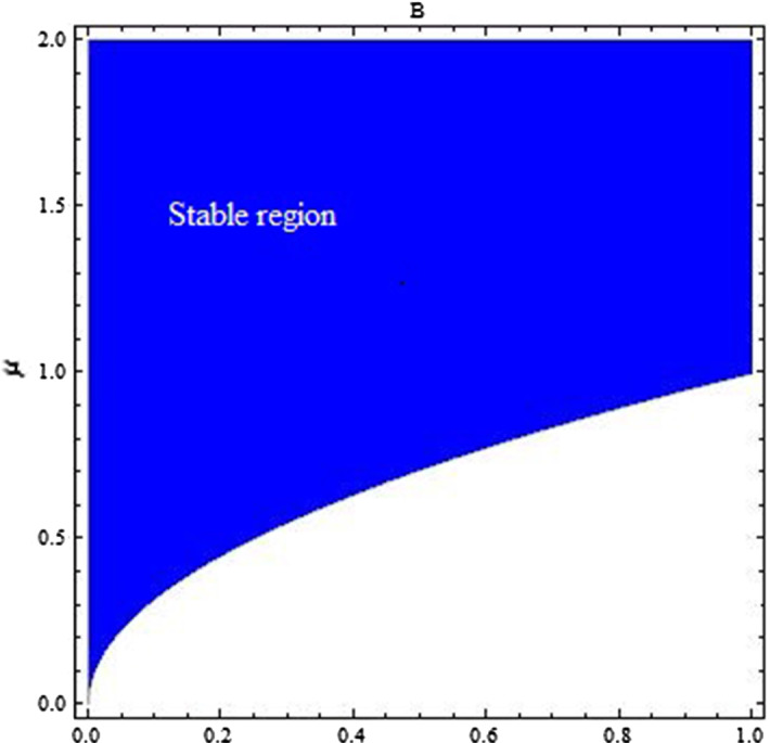
Stable region for $(\frac{B}{\mu },0,0)$ for $a=2,b=10,{\beta }_1=0.99,d=0.4,{\beta }_2=0.01,{\beta }_3=0.80,{\beta }_4=0.60,c_1=1,c_2=2$ , $0<B<1,0<\mu <2$ and $S_0=0.995,E_0=0.38855,Q_0=0.3455$

Fig. 3.

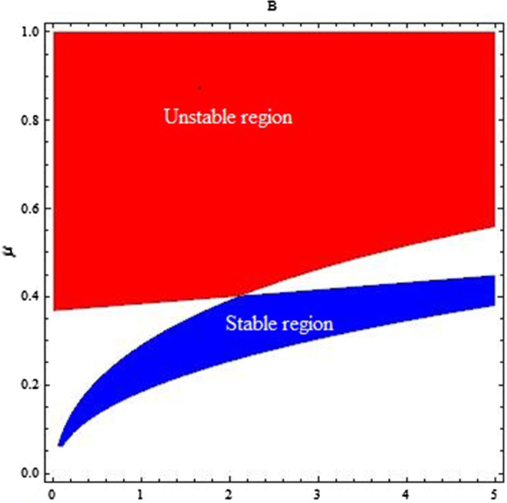
Stable and unstable regions for $\left(\frac{b\mu }{c_2{\beta }_4-\mu },,,0,,,\frac{b{c}_2\left(B,c_2,{\beta }_4,-,\mu ,(B+b\mu )\right)}{\left(\mu ,-,c_2,{\beta }_4\right){}^2}\right)$ for $a=2,b=10,{\beta }_1=0.99,d=0.4,{\beta }_2=0.01,{\beta }_3=0.80,{\beta }_4=0.60,c_1=1,c_2=2$ , $0<B<5,0<\mu <1$ and $S_0=0.995,E_0=0.38855,Q_0=0.3455$

Proposition 3.2

Let $(\frac{B}{\mu },0,0)$ be a equilibrium point of (4) then;

• (i)
  $(\frac{B}{\mu },0,0)$ is a stable equilibrium point if $|{\tau }_1|,|{\tau }_2|,|{\tau }_3|<1$ if and only if

  $$\begin{array}{c}\hfill 0<B<2and{\mu }^2(B+a\mu )>B({\beta }_1(B+a\mu )+\mu {\beta }_2).\end{array}$$
• (ii)
  $(\frac{B}{\mu },0,0)$ is a unstable equilibrium point if

  $$\begin{array}{c}\hfill B>2.\end{array}$$

Consider the equilibrium point $\left(\frac{b\mu }{c_2{\beta }_4-\mu },,,0,,,\frac{b{c}_2\left(B,c_2,{\beta }_4,-,\mu ,(B+b\mu )\right)}{\left(\mu ,-,c_2,{\beta }_4\right){}^2}\right)$ of system (4) and suppose $F_{J_3}$ be the matrix of variation for system (4) about $\left(\frac{b\mu }{c_2{\beta }_4-\mu },,,0,,,\frac{b{c}_2\left(B,c_2,{\beta }_4,-,\mu ,(B+b\mu )\right)}{\left(\mu ,-,c_2,{\beta }_4\right){}^2}\right)$ . Then, $F_{J_3}$ has the following mathematical form:

$$\begin{array}{c}\hfill F_{J_3}=\left(\begin{array}{ccc}1+\frac{\mu (B+b\mu )}{c_2{\beta }_4}+\frac{2b{\mu }^2}{\mu -c_2{\beta }_4}& b\mu \left(\frac{{\beta }_1}{\mu -c_2{\beta }_4},+,\frac{{\beta }_2}{a\mu -b\mu -a{c}_2{\beta }_4}\right)& -\frac{\mu }{c_2}\\ 0& e^{-\mu +\frac{b\mu {\beta }_1}{-\mu +c_2{\beta }_4}+\frac{b\mu {\beta }_2}{(-a+b)\mu +a{c}_2{\beta }_4}+\frac{b{c}_2{\beta }_3\left(\mu ,(B+b\mu ),-,B,c_2,{\beta }_4\right)}{d\left(\mu ,-,c_2,{\beta }_4\right){}^2}}& 0\\ \frac{e^{-2\mu }\left(\mu ,(B+b\mu ),-,B,c_2,{\beta }_4\right)}{{\beta }_4}& -\frac{b{e}^{-2\mu }{c}_1{c}_2{\beta }_3\left(\mu ,(B+b\mu ),-,B,c_2,{\beta }_4\right)}{d\left(\mu ,-,c_2,{\beta }_4\right){}^2}& e^{-2\mu }\end{array}\right).\end{array}$$

Assume that $\mathbb{H}(\psi )$ is characteristic polynomial of Jacobian matrix $F_{J_3}$. Then, characteristic roots of $\mathbb{H}(\psi )=0$ are given by

$$\begin{array}{cc}\hfill {\psi }_1=& \frac{1}{e^{\mu -\frac{b\mu {\beta }_1}{c_2{\beta }_4-\mu }-\frac{b\mu {\beta }_2}{(b-a)\mu +a{c}_2{\beta }_4}-\frac{b{c}_2{\beta }_3\left(\mu ,(B+b\mu ),-,B,c_2,{\beta }_4\right)}{d\left(\mu ,-,c_2,{\beta }_4\right){}^2}}},\hfill \\ \hfill {\psi }_2,{\psi }_3=& \frac{\left(a_{11},\pm ,\sqrt{a_{12}+a_{13}}\right)}{e^{2\mu }2c_2{\beta }_4\left(\mu ,-,c_2,{\beta }_4\right)},\hfill \end{array}$$

where

$$\begin{array}{c}\hfill \left\{\begin{array}{c}{a}_{11}=e^{2\mu }{\mu }^2(B+b\mu )+\mu \left(1,,+,,e^{2\mu },(1-B+b\mu )\right)c_2{\beta }_4-\left(1,,+,,e^{2\mu }\right)c_2^2{\beta }_4^2,\hfill \\ a_{12}=\left(e^{2\mu },{\mu }^2,(B+b\mu ),,+,,c_2,{\beta }_4,\left(\mu ,,+,,e^{2\mu },\mu ,(1-B+b\mu ),,-,,\left(1,,+,,e^{2\mu }\right),c_2,{\beta }_4\right)\right){}^2,\hfill \\ and\hfill \\ a_{13}=4e^{2\mu }{c}_2{\beta }_4\left(c_2,{\beta }_4,,-,,\mu \right)\left({\mu }^2,(1+\mu ),(B+b\mu ),,-,,c_2,{\beta }_4,\left(\mu ,(B-1+2B\mu +b(\mu -1)\mu ),,+,,(B\mu -1),c_2,{\beta }_4\right)\right).\hfill \end{array}\right)\end{array}$$ 7

Proposition 3.3

Let $\left(\frac{b\mu }{c_2{\beta }_4-\mu },,,0,,,\frac{b{c}_2\left(B,c_2,{\beta }_4,-,\mu ,(B+b\mu )\right)}{\left(\mu ,-,c_2,{\beta }_4\right){}^2}\right)$ be a equilibrium point of (4) and ${\psi }_1,$ ${\psi }_2$ and ${\psi }_3$ are characteristic roots for $F_{J_3}$, then $\left(\frac{b\mu }{c_2{\beta }_4-\mu },,,0,,,\frac{b{c}_2\left(B,c_2,{\beta }_4,-,\mu ,(B+b\mu )\right)}{\left(\mu ,-,c_2,{\beta }_4\right){}^2}\right)$ remains stable if

$$\begin{array}{c}\hfill \mu >\frac{b\mu {\beta }_1}{c_2{\beta }_4-\mu }+\frac{b\mu {\beta }_2}{(b-a)\mu +a{c}_2{\beta }_4}+\frac{b{c}_2{\beta }_3\left(\mu ,(B+b\mu ),-,B,c_2,{\beta }_4\right)}{d\left(\mu ,-,c_2,{\beta }_4\right){}^2}\end{array}$$

and

$$\begin{array}{c}\hfill |\left(a_{11},\pm ,\sqrt{a_{12}+a_{13}}\right)|<e^{2\mu }2c_2{\beta }_4\left(\mu ,-,c_2,{\beta }_4\right)\end{array}$$

with $\mu >c_2{\beta }_4$ and $a_{11},a_{12},a_{13}$ are given in (7).

It is prominent that the equilibrium points of mathematical system (4), that is, the solution of system (5) cannot be unique, however, for biological aims; we are concerned to the positive results of (5). Hence, we do not care about exactly how many results are there of system (5). From the system (5), we get

$$\begin{array}{c}\hfill E^{\ast }=-d\left(1,+,\frac{c_1{\beta }_3(b+S^{\ast })}{\mu (b+S^{\ast })+c_2{\beta }_4+S^{\ast }-c_1{\beta }_3(b+S^{\ast })}\right)\end{array}$$

and

$$\begin{array}{c}\hfill Q^{\ast }=\frac{-(d+E^{\ast })}{{\beta }_3}\left(\mu ,-,\left({\beta }_1,+,\frac{{\beta }_2}{(a+S^{\ast })}\right),S^{\ast }\right),\end{array}$$

where $S^{\ast }$ is one of the roots of cubic polynomial:

$$\begin{array}{c}\hfill g(t)=A_{11}{t}^3+B_{11}{t}^2+C_{11}t+D_{11},\end{array}$$ 8

where

$$\begin{array}{c}\hfill \left\{\begin{array}{c}{A}_{11}=\mu (c_1{\beta }_3+c_2{\beta }_4-\mu ),\hfill \\ B_{11}=(B-(a+b)\mu )(\mu -c_1{\beta }_3)-(B-a\mu )c_2{\beta }_4+d{\beta }_1(\mu +(c_1-c_2){\beta }_4),\hfill \\ C_{11}=((a+b)B-ab\mu )(\mu -c_1{\beta }_3)-(d\mu c_1+aB{c}_2){\beta }_4+(\mu +(c_1-c_2){\beta }_4)d{\beta }_2\hfill \\ +((a+b)\mu +a(c_1-c_2){\beta }_4)d{\beta }_1,\hfill \\ D_{11}=(ab(B+d{\beta }_1)+db{\beta }_3)\mu -a{c}_1(bB{\beta }_3+d\mu {\beta }_4).\hfill \end{array}\right)\end{array}$$ 9

We are looking for the unique positive equilibrium point of system (5). For this, we have the following Descartes rule of signs (see [24]).

Lemma 3.1

[24] Let $f_1(x)=b_n{x}^n+b_{n-1}{x}^{n-1}+b_{n-2}{x}^{n-2}+.....+b_{1}x+b_0$ be a polynomial function with real coefficients. Then, the number of positive real roots of $f_1$ is either the same as the number of sign changes for $f_1(x)$ or less than by a positive even integer. Moreover, if f(x) has only one variation in sign, then $f_1$ has exactly one positive real root.

Using Lemma 3.1, we have the following result for existence of unique positive real root of polynomial g(t) given in (8).

Lemma 3.2

Polynomial g(t) in (8) has unique positive real root if one of the following conditions hold:

$i.A_1<0,B_{11}<0,C_{11}<0,D_{11}>0.$

$ii.A_{11}<0,B_{11}>0,C_{11}>0,D_{11}>0.$

Lemma 3.3

Let $S^{\ast }$ is one of the roots of cubic polynomial (8). Then, under the conditions of lemma 3.2, system (1) has one and only positive fixed point if the following conditions are satisfied:

$$\begin{array}{c}\hfill c_1{\beta }_3+c_2{\beta }_4<\mu <(c_2-c_1){\beta }_4\end{array}$$

and

$$\begin{array}{c}\hfill B<\mu .\end{array}$$

Proof

Positive equilibrium point of (4) fulfills algebraic equations same to its continuous counterpart (1). In case of system (1), the evidence is specified in [1].$\square$

Local stability analysis of system (4) about its endemic equilibrium

We consider the Jacobian matrix $F_{J_4}$ of system (4) about unique positive equilibrium point $(S^{\ast },E^{\ast },Q^{\ast }).$

$$\begin{array}{c}\hfill F_{J_4}=\left(\begin{array}{ccc}1+S^{\ast }\left(\frac{{\beta }_2{E}^{\ast }}{{\left(a,+,S^{\ast }\right)}^2-\mu },+,\frac{{\beta }_4{Q}^{\ast }}{{\left(b,+,S^{\ast }\right)}^2}\right)& -S^{\ast }\left({\beta }_1,+,\frac{{\beta }_2}{a+S^{\ast }}\right)& -\frac{{\beta }_4{S}^{\ast }}{b+S^{\ast }}\\ \frac{E^{\ast }\left(a,{\beta }_2,+,{\beta }_1,{\left(a,+,S^{\ast }\right)}^2\right)}{{\left(a,+,S^{\ast }\right)}^2}& \frac{{\left(d,+,E^{\ast }\right)}^2+{\beta }_3{E}^{\ast }{Q}^{\ast }}{{\left(d,+,E^{\ast }\right)}^2}& -\frac{{\beta }_3{E}^{\ast }}{d+E^{\ast }}\\ -\frac{b{c}_2{\beta }_4{Q}^{\ast }}{{\left(b,+,S^{\ast }\right)}^2}& \frac{d{c}_1{\beta }_3{Q}^{\ast }}{{\left(d,+,E^{\ast }\right)}^2}& 1\end{array}\right).\end{array}$$ 10

Moreover, assume that (14) be the characteristic equation of (10). Then, in direction to study the stability analysis of one and only positive equilibrium point, we have the next theorem, which provides us freely confirmable necessary and sufficient situations for all the roots of real polynomial of degree 3 to have magnitude smaller than one (see, Theorem 5 from [25]).

Theorem 4.1

Assume the next third-degree polynomial equation

$$\begin{array}{c}\hfill \mathbb{H}(\omega )={\omega }^3-A_1{\omega }^2+A_2\omega -A_3,\end{array}$$ 11

where $A_1,A_2,A_3\in \mathfrak{R}.$ Then, necessary and sufficient conditions that all roots of (11) lie inside an open disk are given as follows:

$$\begin{array}{c}\hfill \left\{\begin{array}{c}|A_1+A_3|<1+A_2,\hfill \\ |A_1-3A_3|<3-A_2,\hfill \\ {A_3}^2+A_2-A_1{A}_3<1.\hfill \end{array}\right)\end{array}$$ 12

Theorem 4.2

The unique positive equilibrium point $(S^{\ast },E^{\ast },Q^{\ast })$ of system (4) is locally asymptotically stable if the following conditions are satisfied:

$$\begin{array}{c}\hfill \left\{\begin{array}{c}|A_1+A_3|<1+A_2,\hfill \\ |A_1-3A_3|<3-A_2,\hfill \\ {A_3}^2+A_2-A_1{A}_3<1.\hfill \end{array}\right)\end{array}$$

where

$$\begin{array}{c}\hfill \left\{\begin{array}{c}{A}_1=3+\frac{{\beta }_3{E}^{\ast }{Q}^{\ast }}{{\tau }^2}+\left(-,\mu ,+,\frac{{\beta }_2{E}^{\ast }}{{\rho }^2},+,\frac{{\beta }_4{Q}^{\ast }}{{\sigma }^2}\right)S^{\ast },\hfill \\ A_2=3+\frac{d{c}_1{\beta }_3^2{E}^{\ast }{Q}^{\ast }}{{\tau }^3}+S^{\ast }\left(\frac{\left({\rho }^3,{\beta }_1^2,+,\rho ,\left(2,+,(a+\rho ),{\beta }_1\right),{\beta }_2,+,a,{\beta }_2^2\right)E^{\ast }}{{\rho }^3},-,2,\mu ,+,{\beta }_4,Q^{\ast },\left(\frac{\sigma -b{c}_2{\beta }_4}{{\sigma }^3},+,\frac{1}{{\left({\sigma }^{\ast }\right)}^2}\right)\right)\hfill \\ +\frac{{\beta }_3{E}^{\ast }{Q}^{\ast }\left({\rho }^2,{\beta }_4,Q^{\ast },S^{\ast },+,\left(2,{\rho }^2,+,\left(-,\mu ,{\rho }^2,+,{\beta }_2,E^{\ast }\right),S^{\ast }\right),{\left({\sigma }^{\ast }\right)}^2\right)}{{\rho }^2{\tau }^2{\left({\sigma }^{\ast }\right)}^2},\hfill \\ A_3=\frac{1}{{\rho }^3{\sigma }^3{\tau }^3}\left({\rho }^3,{\sigma }^3,\left({\tau }^3,+,{\beta }_3,\left(\tau ,+,d,c_1,{\beta }_3\right),E^{\ast },Q^{\ast }\right),+,\left({\sigma }^3,{\tau }^3,\left({\rho }^3,{\beta }_1^2,+,\rho ,\left(1,+,(a+\rho ),{\beta }_1\right),{\beta }_2,+,a,{\beta }_2^2\right),E^{\ast },-,\mu ,{\rho }^3\right)\right)\hfill \\ -\frac{\rho }{{\rho }^3{\sigma }^3{\tau }^3}\left(b,{\rho }^2,{\tau }^3,c_2,{\beta }_4^2,+,{\sigma }^3,{\beta }_3,\left(\tau ,+,d,c_1,{\beta }_3\right),E^{\ast },\left(\mu ,{\rho }^2,-,{\beta }_2,E^{\ast }\right)\right)\hfill \\ +\frac{1}{{\rho }^3{\sigma }^3{\tau }^3}\left(\sigma ,\tau ,{\beta }_4,\left(-,{\rho }^2,{\tau }^2,+,\left(b,\rho ,\tau ,c_2,\left(\rho ,{\beta }_1,+,{\beta }_2\right),+,d,\sigma ,c_1,\left({\rho }^2,{\beta }_1,+,a,{\beta }_2\right)\right),{\beta }_3,E^{\ast }\right),Q^{\ast }\right)\hfill \\ +\frac{{\rho }^3{\beta }_3{\beta }_4}{{\rho }^3{\sigma }^3{\tau }^3}\left(d,\sigma ,c_1,{\beta }_3,+,\tau ,\left(\sigma ,-,b,c_2,{\beta }_4\right)\right)E^{\ast }{\left(Q^{\ast }\right)}^2{S}^{\ast },\hfill \\ a+S^{\ast }=\rho ,\hfill \\ b+S^{\ast }=\sigma ,\hfill \\ and\hfill \\ d+E^{\ast }=\tau .\hfill \end{array}\right)\end{array}$$ 13

Proof

The Jacobian matrix for system (4) evaluated at unique positive fixed point $(S^{\ast },E^{\ast },Q^{\ast })$ is given by

$$\begin{array}{c}\hfill F_{J_4}=\left(\begin{array}{ccc}1+S^{\ast }\left(\frac{{\beta }_2{E}^{\ast }}{{\left(a,+,S^{\ast }\right)}^2-\mu },+,\frac{{\beta }_4{Q}^{\ast }}{{\left(b,+,S^{\ast }\right)}^2}\right)& -S^{\ast }\left({\beta }_1,+,\frac{{\beta }_2}{a+S^{\ast }}\right)& -\frac{{\beta }_4{S}^{\ast }}{b+S^{\ast }}\\ \frac{E^{\ast }\left(a,{\beta }_2,+,{\beta }_1,{\left(a,+,S^{\ast }\right)}^2\right)}{{\left(a,+,S^{\ast }\right)}^2}& \frac{{\left(d,+,E^{\ast }\right)}^2+{\beta }_3{E}^{\ast }{Q}^{\ast }}{{\left(d,+,E^{\ast }\right)}^2}& -\frac{{\beta }_3{E}^{\ast }}{d+E^{\ast }}\\ -\frac{b{c}_2{\beta }_4{Q}^{\ast }}{{\left(b,+,S^{\ast }\right)}^2}& \frac{d{c}_1{\beta }_3{Q}^{\ast }}{{\left(d,+,E^{\ast }\right)}^2}& 1\end{array}\right).\end{array}$$

Then, characteristic polynomial $\mathbb{H}(\omega )$ from matrix $F_{J_4}$ is given by:

$$\begin{array}{c}\hfill \mathbb{H}(\omega )={\omega }^3-A_1{\omega }^2+A_2\omega -A_3,\end{array}$$ 14

where $A_1,A_2$ and $A_3$ are given in (13). Now, by using Theorem 4.1, the one and only positive equilibrium point $(S^{\ast },E^{\ast },Q^{\ast })$ is locally asymptotically stable if the following inequalities are satisfied:

$$\begin{array}{c}\hfill \left\{\begin{array}{c}|A_1+A_3|<1+A_2,\hfill \\ |A_1-3A_3|<3-A_2,\hfill \\ {A_3}^2+A_2-A_1{A}_3<1.\hfill \end{array}\right)\end{array}$$

$\square$

Period-doubling bifurcation

In this part of article, we examine that quarantined free fixed point of system (4) experience period-doubling bifurcation. For this bifurcation concept, center manifold theorem is applied after the application of normal forms to show the existence and direction of such kind of bifurcation. Freshly, period-doubling bifurcation associated with discrete-time models has been explored by many authors [26–30]

Under the suppositions that $B>\mu$ and $Q_n\to 0,\forall n,$ we study the following set:

$$\begin{array}{c}\hfill {\mathrm{\Phi }}_1=\{a,B,d,{\beta }_1,{\beta }_2\in {\mathfrak{R}}^{+}:\mu =f(\overline{S},\overline{E},a,B,d,{\beta }_1,{\beta }_2)\},\end{array}$$

Then, the quarantined free fixed point $(\overline{S},\overline{E},0)$ of system (4) experiences period-doubling bifurcation such that $\mu$ is taken as bifurcation parameter, and it varies in a slight neighborhood of $\widehat{\mu },$ which is given as

$$\begin{array}{c}\hfill \widehat{\mu }=f(\overline{S},\overline{E},a,B,d,{\beta }_1,{\beta }_2).\end{array}$$

In addition, system (4) is characterized evenly with the next two-dimensional map:

$$\begin{array}{c}\hfill \left(\begin{array}{c}S\\ E\end{array}\right)\to \left(\begin{array}{c}S{e}^{B-{\beta }_{1}E-\frac{{\beta }_{2}E}{a+S}-\mu S}\\ E{e}^{{\beta }_{1}S+\frac{{\beta }_{2}S}{a+S}-\mu }\end{array}\right).\end{array}$$ 15

To discuss and analyze the period-doubling bifurcation for steady state $(\overline{S},\overline{E},0)$ of (15), we suppose that $a,B,d,{\beta }_1,{\beta }_2,\widehat{\mu }\in {\mathrm{\Phi }}_1$. Then, it follows that

$$\begin{array}{c}\hfill \left(\begin{array}{c}S\\ E\end{array}\right)\to \left(\begin{array}{c}S{e}^{B-{\beta }_{1}E-\frac{{\beta }_{2}E}{a+S}-\widehat{\mu }S}\\ E{e}^{{\beta }_{1}S+\frac{{\beta }_{2}S}{a+S}-\widehat{\mu }}\end{array}\right).\end{array}$$ 16

Taking $\overline{\mu }$ as small parameter for bifurcation, then the perturbation of mapping (15) can be described by the next map:

$$\begin{array}{c}\hfill \left(\begin{array}{c}S\\ E\end{array}\right)\to \left(\begin{array}{c}S{e}^{B-{\beta }_{1}E-\frac{{\beta }_{2}E}{a+S}-(\widehat{\mu }+\overline{\mu })S}\\ E{e}^{{\beta }_{1}S+\frac{{\beta }_{2}S}{a+S}-(\widehat{\mu }+\overline{\mu })}\end{array}\right)\end{array}$$ 17

where $|\overline{\mu }|\ll 1$, is a small parameter for perturbation.

Taking $x=S-\overline{S}$ and $y=E-\overline{E}$. Then, from (17)we obtained the next map whose fixed point is at (0, 0) ;

$$\begin{array}{c}\hfill \left(\begin{array}{c}x\\ y\end{array}\right)\to \left(\begin{array}{cc}{\theta }_{11}& {\theta }_{12}\\ {\varphi }_{21}& {\varphi }_{22}\end{array}\right)\left(\begin{array}{c}x\\ y\end{array}\right)+\left(\begin{array}{c}{f}_1(x,y,\overline{\mu })\\ f_2(x,y,\overline{\mu })\end{array}\right),\end{array}$$ 18

where

$$\begin{array}{cc}\hfill f_1(x,y,\overline{\mu })=& {\theta }_{13}{x}^2+{\theta }_{14}xy+{\theta }_{15}x\overline{\mu }+{\theta }_{16}{y}^2+{\theta }_{17}\overline{\mu }y+{\theta }_{18}{\overline{\mu }}^2+{\theta }_{19}{x}^3+{\theta }_{20}{x}^{2}y\hfill \\ \hfill & +{\theta }_{21}\overline{\mu }{x}^2+{\theta }_{22}x{y}^2+{\theta }_{23}xy\overline{\mu }+{\theta }_{24}x{\overline{\mu }}^2+{\theta }_{25}y{\overline{\mu }}^2+{\theta }_{26}{\overline{\mu }}^3+O\left((|x|,+,|y|,+,{|\overline{\mu }|)}^4\right),\hfill \\ \hfill f_2(x,y,\overline{\eta })=& {\varphi }_{13}{x}^2+{\varphi }_{14}xy+{\varphi }_{15}y\overline{\mu }+{\varphi }_{16}{\overline{\mu }}^2+{\varphi }_{17}{x}^3+{\varphi }_{18}{x}^{2}y+{\varphi }_{19}\overline{\mu }{x}^2+{\varphi }_{20}\overline{\mu }xy\hfill \\ \hfill & +{\varphi }_{21}{\overline{\mu }}^{2}x+{\varphi }_{22}y{\overline{\mu }}^2+{\varphi }_{23}{\overline{\mu }}^3+O\left((|x|,+,|y|,+,{|\overline{\mu }|)}^4\right),\hfill \\ \hfill \end{array}$$

with

$$\begin{array}{c}\hfill \left\{\begin{array}{c}{\theta }_{11}=\overline{S}\left(\frac{\overline{E}{\beta }_2}{{(a+\overline{S})}^2},-,\overline{\mu }\right),{\theta }_{12}=-\overline{S}\left({\beta }_1,+,\frac{{\beta }_2}{a+\overline{S}}\right),{\theta }_{13}=\frac{1}{2}\left(\overline{\mu },(\overline{S}\overline{\mu }-2),+,\frac{\overline{E}{\beta }_2\left(2,(a+\overline{S}),(a-\overline{S}(a+\overline{S})\overline{\mu }),+,\overline{E},\overline{S},{\beta }_2\right)}{{(a+\overline{S})}^4}\right),\hfill \\ {\theta }_{14}=\left(-,{\beta }_1,-,\frac{{\beta }_2}{a+\overline{S}}\right)+\frac{\overline{S}{\beta }_2}{{(a+\overline{S})}^2}+\overline{S}\left(\frac{{\beta }_2\overline{E}}{{(a+\overline{S})}^2},-,\overline{\mu }\right)\left(-,{\beta }_1,-,\frac{{\beta }_2}{a+\overline{S}}\right),{\theta }_{15}=\overline{S}\left(\overline{S},\overline{\mu },-,2,-,\frac{\overline{E}\overline{S}{\beta }_2}{{(a+\overline{S})}^2}\right),\hfill \\ {\theta }_{16}=\frac{\overline{S}\left((a+\overline{S}),{\beta }_1,+,{\beta }_2\right){}^2}{2{(a+\overline{S})}^2},{\theta }_{17}=\frac{{\overline{S}}^2\left((a+\overline{S}),{\beta }_1,+,{\beta }_2\right)}{a+\overline{S}},{\theta }_{18}=\frac{{\overline{S}}^3}{2},\hfill \\ {\theta }_{19}=\frac{1}{6}\left({\overline{\mu }}^2,(3-\overline{S}\overline{\mu }),+,\frac{\overline{E}{\beta }_2\left(3,{(a+\overline{S})}^2,\left(-,2,a,-,2,a,(a+\overline{S}),\overline{\mu },+,\overline{S},{(a+\overline{S})}^2,{\overline{\mu }}^2\right),+,\overline{E},{\beta }_2,\left(-,3,(a+\overline{S}),(-a+\overline{S}+\overline{S}(a+\overline{S})\overline{\mu }),+,\overline{E},\overline{S},{\beta }_2\right)\right)}{{(a+\overline{S})}^6}\right),\hfill \\ {\theta }_{20}=\frac{{\beta }_2}{{(a+\overline{S})}^2}+\left(\frac{{\beta }_2\overline{E}}{{(a+\overline{S})}^2},-,\overline{\mu }\right)\left(-,{\beta }_1,-,\frac{{\beta }_2}{a+\overline{S}}\right)-\frac{\overline{S}{\beta }_2}{{(a+\overline{S})}^3}-\frac{S{\beta }_{2}E\left(-,{\beta }_1,-,\frac{{\beta }_2}{a+S}\right)}{{(a+\overline{S})}^3}+\frac{S\left(\frac{{\beta }_2\overline{E}}{{(a+\overline{S})}^2},-,\overline{\mu }\right){\beta }_2}{{(a+\overline{S})}^2}\hfill \\ +\frac{1}{2}\overline{S}\left(\frac{{\beta }_2\overline{E}}{{(a+\overline{S})}^2},-,\overline{\mu }\right){}^2\left(-,{\beta }_1,-,\frac{{\beta }_2}{a+S}\right),{\theta }_{21}=-1+\frac{E{S}^2{\beta }_2}{{(a+S)}^3}+2S\left(\overline{\mu },-,\frac{e{\beta }_2}{{(a+\overline{S})}^2}\right)-\frac{1}{2}{\overline{S}}^2\left(\overline{\mu },-,\frac{\overline{E}{\beta }_2}{{(a+\overline{S})}^2}\right){}^2,\hfill \\ {\theta }_{22}=-\frac{\left((a+\overline{S}),{\beta }_1,+,{\beta }_2\right)\left({(a+\overline{S})}^3,(-1+S\overline{\mu }),{\beta }_1,+,(a+\overline{S}),\left(-,a,+,\overline{S},+,\overline{S},(a+\overline{S}),\overline{\mu },-,\overline{E},\overline{S},{\beta }_1\right),{\beta }_2,-,\overline{E},\overline{S},{\beta }_2^2\right)}{2{(a+\overline{S})}^4},\hfill \\ {\theta }_{23}=2\overline{S}\left({\beta }_1,+,\frac{{\beta }_2}{a+\overline{S}}\right)-\frac{{\overline{S}}^2}{{(a+\overline{S})}^2}+{\overline{S}}^2\left(\frac{{\beta }_2\overline{E}}{{(a+\overline{S})}^2},-,\overline{\mu }\right)\left({\beta }_1,+,\frac{{\beta }_2}{a+\overline{S}}\right),{\theta }_{24}=\frac{1}{2}{\overline{S}}^2\left(3,-,\overline{S},\overline{\mu },+,\frac{\overline{E}\overline{S}{\beta }_2}{{(a+\overline{S})}^2}\right),\hfill \\ {\theta }_{25}=-\frac{{\overline{S}}^3\left((a+\overline{S}),{\beta }_1,+,{\beta }_2\right)}{2(a+\overline{S})},{\theta }_{26}=-\frac{{\overline{S}}^4}{6},\hfill \\ {\varphi }_{11}=\overline{E}\left({\beta }_1,+,\frac{a{\beta }_2}{{(a+\overline{S})}^2}\right),{\varphi }_{12}=1,{\varphi }_{13}=\frac{\overline{E}\left({(a+\overline{S})}^4,{\beta }_1^2,+,2,a,(a+S),\left(-,1,+,(a+S),{\beta }_1\right),{\beta }_2,+,a^2,{\beta }_2^2\right)}{2{(a+S)}^4},{\varphi }_{14}={\beta }_1+\frac{a{\beta }_2}{{(a+\overline{S})}^2},\hfill \\ {\varphi }_{15}=-1,{\varphi }_{16}=\frac{\overline{E}}{2},{\varphi }_{17}=\frac{\overline{E}\left(-,6,\overline{S},{(a+\overline{S})}^2,{\beta }_2,+,6,{(a+\overline{S})}^3,{\beta }_2,-,6,a,(a+\overline{S}),{\beta }_2,\left({(a+\overline{S})}^2,{\beta }_1,+,a,{\beta }_2\right),+,\left({(a+\overline{S})}^2,{\beta }_1,+,a,{\beta }_2\right),{}^3\right)}{6{(a+\overline{S})}^6},\hfill \\ {\varphi }_{18}=\frac{-2a(a+\overline{S}){\beta }_2+\left({(a+\overline{S})}^2,{\beta }_1,+,a,{\beta }_2\right){}^2}{2{(a+\overline{S})}^4},{\varphi }_{19}=-\frac{\overline{E}\left({(a+\overline{S})}^4,{\beta }_1^2,+,2,a,(a+\overline{S}),\left((a+\overline{S}),{\beta }_1,-,1\right),{\beta }_2,+,a^2,{\beta }_2^2\right)}{2{(a+\overline{S})}^4},\hfill \\ {\varphi }_{20}=-{\beta }_1-\frac{a{\beta }_2}{{(a+\overline{S})}^2},{\varphi }_{21}=\frac{1}{2}\overline{E}\left({\beta }_1,+,\frac{a{\beta }_2}{{(a+\overline{S})}^2}\right),{\varphi }_{22}=\frac{1}{2},{\varphi }_{23}=-\frac{\overline{E}}{6}.\hfill \end{array}\right)\end{array}$$

Assume that ${\xi }_1,{\xi }_2$ are eigenvalues for system (15), then we have the following translation;

$$\begin{array}{c}\hfill \left(\begin{array}{c}x\\ y\end{array}\right)=M\left(\begin{array}{c}u\\ v\end{array}\right),\end{array}$$ 19

where

$$\begin{array}{c}\hfill M=\left[\begin{array}{cc}-\overline{S}\left({\beta }_1,+,\frac{{\beta }_2}{a+\overline{S}}\right)& -\overline{S}\left({\beta }_1,+,\frac{{\beta }_2}{a+\overline{S}}\right)\\ \overline{S}\overline{\mu }-\frac{\overline{E}\overline{S}{\beta }_2}{{(a+\overline{S})}^2}-1& {\xi }_2-\overline{S}\left(\frac{\overline{E}{\beta }_2}{{(a+\overline{S})}^2},-,\overline{\mu }\right)\end{array}\right]\end{array}$$

be a nonsingular matrix. By applying transformation (19), the map (18) can be written as:

$$\begin{array}{c}\hfill \left(\begin{array}{c}u\\ v\end{array}\right)\to \left(\begin{array}{cc}-1& 0\\ 0& {\xi }_2\end{array}\right)\left(\begin{array}{c}u\\ v\end{array}\right)+\left(\begin{array}{c}f(u,v,\overline{\mu })\\ g(u,v,\overline{\mu })\end{array}\right),\end{array}$$ 20

where

$$\begin{array}{cc}\hfill f(u,v,\overline{\mu })=& \left(\frac{\left({\xi }_2,-,{\theta }_{11}\right){\theta }_{26}}{{\theta }_{12}\left({\xi }_2,+,1\right)},-,\frac{{\varphi }_{23}}{{\xi }_2+1}\right){\overline{\mu }}^3+\left(\frac{\left({\xi }_2,-,{\theta }_{11}\right){\theta }_{24}}{{\theta }_{12}\left({\xi }_2,+,1\right)},-,\frac{{\varphi }_{21}}{{\xi }_2+1}\right){\overline{\mu }}^{2}x\hfill \\ \hfill & +\left(\frac{\left({\xi }_2,-,{\theta }_{11}\right){\theta }_{25}}{{\theta }_{12}\left({\xi }_2,+,1\right)},-,\frac{{\varphi }_{22}}{{\xi }_2+1}\right){\overline{\mu }}^{2}y+\left(\frac{\left({\xi }_2,-,{\theta }_{11}\right){\theta }_{18}}{{\theta }_{12}\left({\xi }_2,+,1\right)},-,\frac{{\varphi }_{16}}{{\xi }_2+1}\right){\overline{\mu }}^2\hfill \\ \hfill & +\left(\frac{\left({\xi }_2,-,{\theta }_{11}\right){\theta }_{21}}{{\theta }_{12}\left({\xi }_2,+,1\right)},-,\frac{{\varphi }_{19}}{{\xi }_2+1}\right)\overline{\mu }{x}^2+\left(\frac{\left({\xi }_2,-,{\theta }_{11}\right){\theta }_{23}}{{\theta }_{12}\left({\xi }_2,+,1\right)},-,\frac{{\varphi }_{20}}{{\xi }_2+1}\right)\overline{\mu }xy\hfill \\ \hfill & +\frac{\left({\xi }_2,-,{\theta }_{11}\right){\theta }_{15}\overline{\mu }x}{{\theta }_{12}\left({\xi }_2,+,1\right)}+\left(\frac{\left({\xi }_2,-,{\theta }_{11}\right){\theta }_{17}}{{\theta }_{12}\left({\xi }_2,+,1\right)},-,\frac{{\varphi }_{15}}{{\xi }_2+1}\right)y\overline{\mu }\hfill \\ \hfill & +\left(\frac{\left({\xi }_2,-,{\theta }_{11}\right){\theta }_{19}}{{\theta }_{12}\left({\xi }_2,+,1\right)},-,\frac{{\varphi }_{17}}{{\xi }_2+1}\right)x^3+\left(\frac{\left({\xi }_2,-,{\theta }_{11}\right){\theta }_{20}}{{\theta }_{12}\left({\xi }_2,+,1\right)},-,\frac{{\varphi }_{18}}{{\xi }_2+1}\right)x^{2}y\hfill \\ \hfill & +\left(\frac{\left({\xi }_2,-,{\theta }_{11}\right){\theta }_{13}}{{\theta }_{12}\left({\xi }_2,+,1\right)},-,\frac{{\varphi }_{13}}{{\xi }_2+1}\right)x^2+\frac{\left({\xi }_2,-,{\theta }_{11}\right){\theta }_{22}x{y}^2}{{\theta }_{12}\left({\xi }_2,+,1\right)}\hfill \\ \hfill & +\left(\frac{\left({\xi }_2,-,{\theta }_{11}\right){\theta }_{14}}{{\theta }_{12}\left({\xi }_2,+,1\right)},-,\frac{{\varphi }_{14}}{{\xi }_2+1}\right)xy+\frac{\left({\xi }_2,-,{\theta }_{11}\right){\theta }_{16}{y}^2}{{\theta }_{12}\left({\xi }_2,+,1\right)}\hfill \\ \hfill & +O\left((|u|,+,|v|,+,{|\overline{\mu }|)}^4\right),\hfill \\ \hfill g(u,v,\overline{\mu })=& \left(\frac{\left(1,+,{\theta }_{11}\right){\theta }_{26}}{{\theta }_{12}\left({\xi }_2,+,1\right)},+,\frac{{\varphi }_{23}}{{\xi }_2+1}\right){\overline{\mu }}^3+\left(\frac{\left(1,+,{\theta }_{11}\right){\theta }_{24}}{{\theta }_{12}\left({\xi }_2,+,1\right)},+,\frac{{\varphi }_{21}}{{\xi }_2+1}\right){\overline{\mu }}^{2}x\hfill \\ \hfill & +\left(\frac{\left(1,+,{\theta }_{11}\right){\theta }_{25}}{{\theta }_{12}\left({\xi }_2,+,1\right)},+,\frac{{\varphi }_{22}}{{\xi }_2+1}\right){\overline{\mu }}^{2}y+\left(\frac{\left(1,+,{\theta }_{11}\right){\theta }_{18}}{{\theta }_{12}\left({\xi }_2,+,1\right)},+,\frac{{\varphi }_{16}}{{\xi }_2+1}\right){\overline{\mu }}^2\hfill \\ \hfill & +\left(\frac{\left(1,+,{\theta }_{11}\right){\theta }_{21}}{{\theta }_{12}\left({\xi }_2,+,1\right)},+,\frac{{\varphi }_{19}}{{\xi }_2+1}\right)\overline{\mu }{x}^2+\left(\frac{\left(1,+,{\theta }_{11}\right){\theta }_{23}}{{\theta }_{12}\left({\xi }_2,+,1\right)},+,\frac{{\varphi }_{20}}{{\xi }_2+1}\right)\overline{\mu }xy\hfill \\ \hfill & +\frac{\left(1,+,{\theta }_{11}\right){\theta }_{15}\overline{\mu }x}{{\theta }_{12}\left({\xi }_2,+,1\right)}+\left(\frac{\left(1,+,{\theta }_{11}\right){\theta }_{17}}{{\theta }_{12}\left({\xi }_2,+,1\right)},+,\frac{{\varphi }_{15}}{{\xi }_2+1}\right)y\overline{\mu }+\left(\frac{\left(1,+,{\theta }_{11}\right){\theta }_{19}}{{\theta }_{12}\left({\xi }_2,+,1\right)},+,\frac{{\varphi }_{17}}{{\xi }_2+1}\right)x^3\hfill \\ \hfill & +\left(\frac{\left(1,+,{\theta }_{11}\right){\theta }_{20}}{{\theta }_{12}\left({\xi }_2,+,1\right)},+,\frac{{\varphi }_{18}}{{\xi }_2+1}\right)x^{2}y+\left(\frac{\left(1,+,{\theta }_{11}\right){\theta }_{13}}{{\theta }_{12}\left({\xi }_2,+,1\right)},+,\frac{{\varphi }_{13}}{{\xi }_2+1}\right)x^2+\frac{\left(1,+,{\theta }_{11}\right){\theta }_{22}x{y}^2}{{\theta }_{12}\left({\xi }_2,+,1\right)}\hfill \\ \hfill & +\left(\frac{\left(1,+,{\theta }_{11}\right){\theta }_{14}}{{\theta }_{12}\left({\xi }_2,+,1\right)},+,\frac{{\varphi }_{14}}{{\xi }_2+1}\right)xy+\frac{\left(1,+,{\theta }_{11}\right){\theta }_{16}{y}^2}{{\theta }_{12}\left({\xi }_2,+,1\right)}+O\left((|u|,+,|v|,+,{|\overline{\mu }|)}^4\right),\hfill \end{array}$$

where,

$$\begin{array}{c}\hfill x={\theta }_{12}(u+v),y=-(1+{\theta }_{11})u+({\xi }_2-{\theta }_{11})v.\end{array}$$

Assume that ${\mho }^c(0,0,0)$ be the center manifold of (20) intended at (0, 0) in a smallest neighborhood of $\overline{\eta }=0.$ Then, ${\mho }^c(0,0,0)$ can be estimated as follows:

$$\begin{array}{c}\hfill {\mho }^c(0,0,0)=\left\{(u,v,\overline{\mu }),\in ,{\mathbb{R}}^3,:,v,=,M_{11},u^2,+,M_{12},u,\overline{\mu },+,M_{13},{\overline{\mu }}^2,+,O,\left((|\overline{\mu }|,+,{|u|)}^3\right)\right\},\end{array}$$

where

$$\begin{array}{cc}\hfill M_{11}=& \frac{1}{1-{\xi }_2}\left(\left(\frac{\left(1,+,{\theta }_{11}\right){\theta }_{13}}{{\theta }_{12}\left({\xi }_2,+,1\right)},+,\frac{{\varphi }_{13}}{{\xi }_2+1}\right),{{\theta }_{12}}^2,-,\left(\frac{\left(1,+,{\theta }_{11}\right){\theta }_{14}}{{\theta }_{12}\left({\xi }_2,+,1\right)},+,\frac{{\varphi }_{14}}{{\xi }_2+1}\right),{\theta }_{12},\left(1,+,{\theta }_{11}\right)\right)\hfill \\ \hfill & +\frac{1}{1-{\xi }_2}\frac{\left(1,+,{\theta }_{11}\right){\theta }_{16}{\left(1,+,{\theta }_{11}\right)}^2}{{\theta }_{12}\left({\xi }_2,+,1\right)},\hfill \\ \hfill M_{12}=& \frac{1}{1-{\xi }_2}\left(\frac{\left(1,+,{\theta }_{11}\right){\theta }_{15}}{{\xi }_2+1},-,\left(\frac{\left(1,+,{\theta }_{11}\right){\theta }_{17}}{{\theta }_{12}\left({\xi }_2,+,1\right)},+,\frac{{\varphi }_{15}}{{\xi }_2+1}\right),\left(1,+,{\theta }_{11}\right)\right),\hfill \\ \hfill M_{13}=& \frac{1}{1-{\xi }_2}\left(\frac{\left(1,+,{\theta }_{11}\right){\theta }_{18}}{{\theta }_{12}\left({\xi }_2,+,1\right)},+,\frac{{\varphi }_{16}}{{\xi }_2+1}\right).\hfill \end{array}$$

Now, the map restricted to set ${\mho }^c(0,0,0)$ is described as follows:

$$\begin{array}{c}\hfill G:u\to -u+k_{11}{u}^2+k_{12}u\overline{\mu }+k_{13}{u}^2\overline{\mu }+k_{14}u{\overline{\mu }}^2+k_{15}{u}^3+O\left((|u|,+,{|\overline{\mu }|)}^4\right),\end{array}$$

where

$$\begin{array}{cc}\hfill k_{11}=& \left(\frac{\left({\xi }_2,-,{\theta }_{11}\right){\theta }_{13}}{{\theta }_{12}\left({\xi }_2,+,1\right)},-,\frac{{\varphi }_{13}}{{\xi }_2+1}\right){{\theta }_{12}}^2-\left(\frac{\left({\xi }_2,-,{\theta }_{11}\right){\theta }_{14}}{{\theta }_{12}\left({\xi }_2,+,1\right)},-,\frac{{\varphi }_{14}}{{\xi }_2+1}\right){\theta }_{12}\left(1,+,{\theta }_{11}\right)\hfill \\ \hfill & +\frac{\left({\xi }_2,-,{\theta }_{11}\right){\theta }_{16}{\left(1,+,{\theta }_{11}\right)}^2}{{\theta }_{12}\left({\xi }_2,+,1\right)},\hfill \\ \hfill k_{12}=& \frac{\left({\xi }_2,-,{\theta }_{11}\right){\theta }_{15}}{{\xi }_2+1}-\left(\frac{\left({\xi }_2,-,{\theta }_{11}\right){\theta }_{17}}{{\theta }_{12}\left({\xi }_2,+,1\right)},-,\frac{{\varphi }_{15}}{{\xi }_2+1}\right)\left(1,+,{\theta }_{11}\right),\hfill \\ \hfill k_{13}=& \left(\frac{\left({\xi }_2,-,{\theta }_{11}\right){\theta }_{21}}{{\theta }_{12}\left({\xi }_2,+,1\right)},-,\frac{{\varphi }_{19}}{{\xi }_2+1}\right){{\theta }_{12}}^2-\left(\frac{\left({\xi }_2,-,{\theta }_{11}\right){\theta }_{23}}{{\theta }_{12}\left({\xi }_2,+,1\right)},-,\frac{{\varphi }_{20}}{{\xi }_2+1}\right){\theta }_{12}\left(1,+,{\theta }_{11}\right)\hfill \\ \hfill & +\frac{\left({\xi }_2,-,{\theta }_{11}\right){\theta }_{15}{M}_1}{{\xi }_2+1}+\left(\frac{\left({\xi }_2,-,{\theta }_{11}\right){\theta }_{17}}{{\theta }_{12}\left({\xi }_2,+,1\right)},-,\frac{{\varphi }_{15}}{{\xi }_2+1}\right)\left({\xi }_2,-,{\theta }_{11}\right)M_1\hfill \\ \hfill & +2\left(\frac{\left({\xi }_2,-,{\theta }_{11}\right){\theta }_{13}}{{\theta }_{12}\left({\xi }_2,+,1\right)},-,\frac{{\varphi }_{13}}{{\xi }_2+1}\right){{\theta }_{12}}^2{M}_2+\left(\frac{\left({\xi }_2,-,{\theta }_{11}\right){\theta }_{14}}{{\theta }_{12}\left({\xi }_2,+,1\right)},-,\frac{{\varphi }_{14}}{{\xi }_2+1}\right){\theta }_{12}\left({\xi }_2,-,{\theta }_{11}\right)M_2\hfill \\ \hfill & -\left(\frac{\left({\xi }_2,-,{\theta }_{11}\right){\theta }_{14}}{{\theta }_{12}\left({\xi }_2,+,1\right)},-,\frac{{\varphi }_{14}}{{\xi }_2+1}\right){\theta }_{12}{M}_2\left(1,+,{\theta }_{11}\right)-2\frac{\left({\xi }_2,-,{\theta }_{11}\right){\theta }_{16}\left(1,+,{\theta }_{11}\right)\left({\xi }_2,-,{\theta }_{11}\right)M_2}{{\theta }_{12}\left({\xi }_2,+,1\right)}\hfill \\ \hfill k_{14}=& \left(\frac{\left({\xi }_2,-,{\theta }_{11}\right){\theta }_{24}}{{\theta }_{12}\left({\xi }_2,+,1\right)},-,\frac{{\varphi }_{21}}{{\xi }_2+1}\right){\theta }_{12}-\left(\frac{\left({\xi }_2,-,{\theta }_{11}\right){\theta }_{25}}{{\theta }_{12}\left({\xi }_2,+,1\right)},-,\frac{{\varphi }_{22}}{{\xi }_2+1}\right)\left(1,+,{\theta }_{11}\right)\hfill \\ \hfill & +\frac{\left({\xi }_2,-,{\theta }_{11}\right){\theta }_{15}{M}_2}{{\xi }_2+1}+\left(\frac{\left({\xi }_2,-,{\theta }_{11}\right){\theta }_{17}}{{\theta }_{12}\left({\xi }_2,+,1\right)},-,\frac{{\varphi }_{15}}{{\xi }_2+1}\right)\left({\xi }_2,-,{\theta }_{11}\right)M_2\hfill \\ \hfill & +2\left(\frac{\left({\xi }_2,-,{\theta }_{11}\right){\theta }_{13}}{{\theta }_{12}\left({\xi }_2,+,1\right)},-,\frac{{\varphi }_{13}}{{\xi }_2+1}\right){{\theta }_{12}}^2{M}_3-2\frac{\left({\xi }_2,-,{\theta }_{11}\right){\theta }_{16}\left(1,+,{\theta }_{11}\right)\left({\xi }_2,-,{\theta }_{11}\right)M_3}{{\theta }_{12}\left({\xi }_2,+,1\right)}\hfill \\ \hfill & +\left(\frac{\left({\xi }_2,-,{\theta }_{11}\right){\theta }_{14}}{{\theta }_{12}\left({\xi }_2,+,1\right)},-,\frac{{\varphi }_{14}}{{\xi }_2+1}\right){\theta }_{12}\left({\xi }_2,-,{\theta }_{11}\right)M_3-\left(\frac{\left({\xi }_2,-,{\theta }_{11}\right){\theta }_{14}}{{\theta }_{12}\left({\xi }_2,+,1\right)},-,\frac{{\varphi }_{14}}{{\xi }_2+1}\right){\theta }_{12}{M}_3\left(1,+,{\theta }_{11}\right),\hfill \\ \hfill k_{15}=& \frac{\left({\xi }_2,-,{\theta }_{11}\right){\theta }_{26}}{{\theta }_{12}\left({\xi }_2,+,1\right)}-\frac{{\varphi }_{23}}{{\xi }_2+1}+\frac{\left({\xi }_2,-,{\theta }_{11}\right){\theta }_{15}{M}_3}{{\xi }_2+1}+\left(\frac{\left({\xi }_2,-,{\theta }_{11}\right){\theta }_{17}}{{\theta }_{12}\left({\xi }_2,+,1\right)},-,\frac{{\varphi }_{15}}{{\xi }_2+1}\right)\left({\xi }_2,-,{\theta }_{11}\right)M_3.\hfill \end{array}$$

Next, we have the following real numbers:

$$\begin{array}{cc}\hfill L_{11}=& {\left(\frac{{\partial }^2{f}_1}{\partial u\partial \overline{\mu }},+,\frac{1}{2},\frac{\partial G}{\partial \overline{\mu }},\frac{{\partial }^{2}G}{\partial u^2}\right)}_{(0,0)}=\frac{\left(\left(1,+,{\theta }_{11}\right),{\theta }_{17},-,{\theta }_{12},{\theta }_{15}\right)\left({\theta }_{11},-,{\xi }_2\right)+\left(1,+,{\theta }_{11}\right){\theta }_{12}{\varphi }_{15}}{{\theta }_{12}\left(1,+,{\xi }_2\right)}\ne 0,\hfill \\ \hfill L_{12}=& {\left({\left(\frac{1}{2},\frac{{\partial }^{2}G}{\partial u^2}\right)}^2,+,\frac{1}{6},\frac{{\partial }^{3}G}{\partial u^3}\right)}_{(0,0)}={k_{11}}^2+k_{15}\ne 0.\hfill \end{array}$$

Hence, by aforementioned study we have the next conclusive theorem related to the existence of period-doubling bifurcation of system (4) about $(\overline{S},\overline{E},0).$

Theorem 5.1

If $L_{12}\ne 0$, then system (4) undergoes period-doubling bifurcation at the isolation free equilibrium $(\overline{S},\overline{E},0)$ when parameter $\mu$ varies in small neighborhood of $\overline{\mu }.$ Furthermore, if $L_{12}>0$, then the period-two orbits that bifurcate from $(\overline{S},\overline{E},0)$ are stable, and if $L_{12}<0$, then these orbits are unstable.

Neimark–Sacker bifurcation

This section is related to the bifurcation analysis of the system (4) about $(S^{\ast },E^{\ast },Q^{\ast }).$ Where all conditions for existence and positivity of $(S^{\ast },E^{\ast },Q^{\ast })$ are given in Lemmas 2.3 and 3.3. Here, we will discuss the Neimark–Sacker bifurcation experienced by system (4) about $(S^{\ast },E^{\ast },Q^{\ast })$ under some mathematical conditions. Bifurcation is the mathematical phenomena produced in any system due to creation of very small change in stability of system. Mathematically, bifurcation arises whenever parameters are varied in very least neighborhood of equilibrium point. Moreover, for further study of bifurcation theory and to understand this surprising behavior of a discrete-time mathematical system one can see [31–34]. We deliberate the Neimark–Sacker Bifurcation for positive equilibrium point $(S^{\ast },E^{\ast },Q^{\ast })$ of system (4) by using an obvious criterion for Neimark–Sacker Bifurcation and compelling $\mu$ as a bifurcation parameter. Due to appearance of Neimark–Sacker Bifurcation, closed invariant circles are formed. Equally, one can find some lonely orbits of periodic performance alongside with paths that cover the invariant circle tightly. The bifurcation can be supercritical or subcritical causing in a stable or unstable closed invariant curve, correspondingly. In command to study the Neimark–Sacker bifurcation in system (4), we have the next obvious standard of Hopf bifurcation [35]. By means of this standard, one can catch the presence of Neimark–Sacker bifurcation deprived of finding the eigenvalues.

Lemma 6.1

(see [35]) Consider an m-dimensional discrete dynamical system $Y_{K+1}=g_{\alpha }(Y_K)$, where $\alpha \in \mathfrak{R}$ is bifurcation parameter. Let $Y^{\ast }$ be a fixed point of $g_{\alpha }$ and the characteristic polynomial for Jacobian matrix $J(Y^{\ast })={(s_{\mathit{ij}})}_{m\times m}$ of m-dimensional map $g_{\alpha }$ is given by

$$\begin{array}{c}\hfill {\mathbb{H}}_{\alpha }(\kappa )={\kappa }^m+b_1{\kappa }^{m-1}+b_2{\kappa }^{m-2}+........+b_{m-1}\kappa +b_m\end{array}$$ 21

where $b_i=b_i(\alpha ,s),$ $i=1,2,3,....,m$ and s is control parameter or another parameter to be determined. Let ${\mathrm{\Delta }}_0^{\pm }(\alpha ,s)=1,{\mathrm{\Delta }}_1^{\pm }(\alpha ,s),{\mathrm{\Delta }}_2^{\pm }(\alpha ,s),.....,{\mathrm{\Delta }}_m^{\pm }(\alpha ,s).$ be the sequence of determinants defined by ${\mathrm{\Delta }}_i^{\pm }(\alpha ,s)=det(N_1\pm N_2),i=1,2,3,....,m$ where

$$\begin{array}{cc}\hfill N_1=& \left(\begin{array}{ccccc}1& b_1& b_2& ....& b_{i-1}\\ 0& 1& b_1& ....& b_{i-2}\\ 0& 0& 1& ....& b_{i-3}\\ ....& ....& ....& ....& ....\\ 0& 0& 0& ....& 1\end{array}\right)\hfill \end{array}$$ 22

$$\begin{array}{cc}\hfill N_2=& \left(\begin{array}{ccccc}{b}_{m-i+1}& b_{m-i+2}& ....& b_{m-1}& b_m\\ b_{m-i+2}& b_{m-i+3}& ....& b_m& 0\\ b_{m-i+3}& b_{m-i+4}& ....& 0& 0\\ ....& ....& ....& ....& ....\\ b_m& 0& 0& ....& 0\end{array}\right).\hfill \end{array}$$ 23

Moreover, the following conditions are satisfied:

$C_1$

Eigenvalue assignment: ${\mathrm{\Delta }}_{m-1}^{-}({\alpha }_0,s)=0,{\mathrm{\Delta }}_{m-1}^{+}({\alpha }_0,s)>0,{\mathbb{H}}_{{\alpha }_0}(1)>0$, ${(-1)}^m{\mathbb{H}}_{{\alpha }_0}(-1)>0$, ${\mathrm{\Delta }}_i^{\pm }({\alpha }_0,s)>0,i=m-3,m-5,m-7,....,1$ or $i=m-3,m-5,m-7,....,2$ when m is even or odd, respectively.

$C_2$

Transversality condition: ${\left[\frac{d}{d\alpha },({\mathrm{\Delta }}_{m-1}^{-}(\alpha ,s))\right]}_{\alpha ={\alpha }_0}\ne 0$

$C_3$

Nonresonance condition: $cos(\frac{2\pi }{n})\ne \psi ,$ or resonance condition $cos(\frac{2\pi }{n})=\psi ,$ where $n=3,4,5,....,$ and $\psi =\frac{-1+0.5{\mathbb{H}}_{{\alpha }_0}(1){\mathrm{\Delta }}_{m-3}^{-}({\alpha }_0,s)}{{\mathrm{\Delta }}_{m-2}^{+}({\alpha }_0,s)}.$ Then, Neimark–Sacker bifurcation exits at ${\alpha }_0.$

The following result shows that system (4) undergoes Neimark–Sacker bifurcation if we take $\alpha$ as bifurcation parameter.

Theorem 6.1

The unique positive equilibrium point of system (4) undergoes Neimark–Sacker bifurcation if the following conditions hold:

$$\begin{array}{c}\hfill \left\{\begin{array}{c}1-A_2+A_3(A_1-A_3)=0,\hfill \\ 1+A_2-A_3(A_1+A_3)>0,\hfill \\ 1+A_1+A_2+A_3>0,\hfill \\ 1-A_1+A_2-A_3>0.\hfill \end{array}\right)\end{array}$$

where, $A_1,A_2$ and $A_3$ are given in (13).

Proof

According to Lemma 6.1, for $m=3$, we have in (14) the characteristic polynomial of system (4) evaluated at its unique positive equilibrium, then we obtain the following equalities and inequalities:

$$\begin{array}{c}\hfill \left\{\begin{array}{c}{\mathrm{\Delta }}_2^{-}(\mu )=1-A_2+A_3(A_1-A_3)=0,\hfill \\ {\mathrm{\Delta }}_2^{+}(\mu )=1+A_2-A_3(A_1+A_3)>0,\hfill \\ {\mathbb{H}}_{\mu }(1)=1+A_1+A_2+A_3>0,\hfill \\ {(-1)}^3{\mathbb{H}}_{\mu }(-1)=1-A_1+A_2-A_3>0.\hfill \end{array}\right)\end{array}$$

$\square$

Remark 6.1

The arithmetical rule for $\mu$ at which Neimark–Sacker bifurcation arises can be established by finding the solutions of the equation ${\mathrm{\Delta }}_2^{-}(\mu )=0$.

Modified hybrid control of Bifurcation and Chaos

Control of bifurcation and chaos in mathematical models is considered as a key element for population models mainly when these models are associated with biological interactions and breeding of different species. Generally discrete-time mathematical systems are more complex to analyze as compared to continuous one. It is necessary that the population does not experience any irregular situation. Hence, to avoid these irregularities a chaos controlling technique must be implemented. In this part of manuscript, we study a feedback control strategy with parameter perturbation to move unstable and irregular trajectories toward the stable trajectories. The most useful and well-known method in the field of chaos is given by Ott et al. [36] to control period-doubling bifurcation, which is known as OGY method. Latter on, numerous strategic control methods are developed (see [22, 37]). Here, we present a modified hybrid control method to control the Neimark–Sacker bifurcation and chaos. Furthermore, this mathematical method is well applicable to every discrete-time system experiencing the period-doubling bifurcation and chaos. Originally, hybrid method was proposed by Liu et al. [27]. Moreover, it was developed to control the period-doubling bifurcation (see [26–30]). Here, we have used the modified hybrid control technique [22] to control Neimark–Sacker bifurcation. Moreover, this technique is much better then old techniques of control. Consider the following n-dimensional discrete dynamical system:

$$\begin{array}{c}\hfill Z_{n+1}=g(Z_n,\ell )\end{array}$$ 24

with $Z_n\in {\mathfrak{R}}^n$, $n\in Z.$ Suppose $\ell \in \mathfrak{R}$ is parameter for which system (24) experiences the bifurcation. The purpose of proposing the modified technique for controlling the bifurcation is to regain the maximum range of stable region in (24) by reduction in length of unstable region. Hence, we present the following generalized hybrid control technique by applying state feedback along with parameter perturbation;

$$\begin{array}{c}\hfill Z_{n+k}={\theta }^3{g}^{(ħ)}(Z_n,\ell )+(1-{\theta }^3)Z_n\end{array}$$ 25

where $ħ>0$ is in Z and $0<\theta <1$ is parameter for controlling the bifurcation appearing in (25). In addition, $g^{(ħ)}$ is kth iterative value of g(.). By application of (25) on system (4), we get the following system;

$$\begin{array}{c}\hfill \begin{array}{cc}\hfill S_{n+1}& ={\theta }^3\left(S_n,e^{B-{\beta }_1{E}_n-\frac{{\beta }_2{E}_n}{a+S_n}-\frac{{\beta }_4{Q}_n}{b+S_n}-\mu S_n}\right)+(1-{\theta }^3)S_n,\hfill \\ \hfill E_{n+1}& ={\theta }^3\left(E_n,e^{{\beta }_1{S}_n+\frac{{\beta }_2{S}_n}{a+S_n}-\frac{{\beta }_3{Q}_n}{d+E_n}-\mu }\right)+(1-{\theta }^3)E_n,\hfill \\ \hfill Q_{n+1}& ={\theta }^3\left(Q_n,e^{\frac{c_1{\beta }_3{E}_n}{d+E_n}+\frac{c_2{\beta }_4{S}_n}{b+S_n}-\mu }\right)+(1-{\theta }^3)Q_n\hfill \end{array}\end{array}$$ 26

Furthermore, the system (26) and system (4) have same constant solutions. Additionally, the Jacobian matrix of (26) about $(S^{\ast },E^{\ast },Q^{\ast })$ is given as follows:

$$\begin{array}{c}\hfill \left(\begin{array}{ccc}1+{\theta }^3{S}^{\ast }\left(\mu ,-,\frac{{\beta }_2{e}^{\ast }}{{\left(a,+,S^{\ast }\right)}^2},-,\frac{{\beta }_4{Q}^{\ast }}{{\left(b,+,S^{\ast }\right)}^2}\right)& -{\theta }^3{S}^{\ast }\left({\beta }_1,+,\frac{{\beta }_2}{a+S^{\ast }}\right)& -\frac{{\theta }^3{\beta }_4{S}^{\ast }}{b+S^{\ast }}\\ \frac{{\theta }^3{E}^{\ast }\left(a,{\beta }_2,+,{\beta }_1,{\left(a,+,S^{\ast }\right)}^2\right)}{{\left(a,+,S^{\ast }\right)}^2}& 1-{\theta }^3+\frac{{\theta }^3\left({\left(d,+,E^{\ast }\right)}^2,+,{\beta }_3,E^{\ast },Q^{\ast }\right)}{{\left(d,+,E^{\ast }\right)}^2}& -\frac{{\theta }^3{\beta }_3{E}^{\ast }}{d+E^{\ast }}\\ -\frac{b{\theta }^3{c}_2{\beta }_4{Q}^{\ast }}{{\left(b,+,S^{\ast }\right)}^2}& \frac{d{\theta }^3{c}_1{\beta }_3{Q}^{\ast }}{{\left(d,+,e^{\ast }\right)}^2}& 1\end{array}\right).\end{array}$$ 27

The one and only positive equilibrium point $(S^{\ast },E^{\ast },Q^{\ast })$ of the controlled system (26) is locally asymptotically stable, if all solutions of the characteristic polynomial of (27) lie inside $D_1.$ Where $D_1$ is an open unit disk.

Numerical simulation

In this part of article, the numerical analysis for the dynamics of (4) is provide. Moreover, this study is the direct verification of our theoretical analysis and analytic results which we proved in previous sections.

Example 8.1

Assume that $a=2,b=10,{\beta }_1=0.99,d=0.4,{\beta }_2=0.01,{\beta }_3=0.80,{\beta }_4=0.60,c_1=1,c_2=2$ and $B>0.$ Then, the discrete-time mathematical system (4) takes the following form:

$$\begin{array}{c}\hfill \begin{array}{cc}\hfill S_{n+1}& =S_n{e}^{B-0.99E_n-\frac{0.01E_n}{2+S_n}-\frac{0.60Q_n}{10+S_n}-\mu S_n},\hfill \\ \hfill E_{n+1}& =E_n{e}^{0.99S_n+\frac{0.01S_n}{2+S_n}-\frac{0.80Q_n}{0.4+E_n}-\mu },\hfill \\ \hfill Q_{n+1}& =Q_n{e}^{\frac{0.80E_n}{0.4+E_n}+\frac{2{(0.60S)}_n}{10+S_n}-\mu },\hfill \end{array}\end{array}$$ 28

where $\mu >0$ and $S_0=0.91059,E_0=0.38854,Q_0=0.3549$ are initial conditions. In this case, the graphical behavior of both population variables is shown in (Fig. 4). In (Fig. 4c), maximum Lyapunov exponents for the existence of bifurcation are given. In (Fig. 5), some phase portraits are given for variations of $\mu >0$. Hence, it can be easily seen that there exists the Neimark–Sacker bifurcation for large range of bifurcation parameter $\mu .$ For aforementioned values of parameters, one can obtain the Jacobian matrix $F_{J_3}$ as follows:

$$\begin{array}{c}\hfill F_{J_3}=\left(\begin{array}{ccc}1+0.91059(0.0021294-\mu )& -0.904613& -0.0500756\\ 0.286336& 1.1728& -0.335248\\ -0.0357759& 0.239551& 1\end{array}\right).\end{array}$$

Moreover, the characteristic equation $\mathbb{H}(\psi )=0$ for $F_{J_3}$ has the following coefficients:

$$\begin{array}{cc}\hfill A_1=& 3.17946-0.91059\mu ,\hfill \\ \hfill A_2=& 3.68735-1.97853\mu ,\hfill \\ \hfill A_3=& 1.58237-1.1377\mu .\hfill \end{array}$$

Moreover, the equilibrium point $(S^{\ast },E^{\ast },Q^{\ast })$ will be locally asymptotically stable for

$$\begin{array}{c}\hfill 0.37858611389735736<\mu <1.0675487017977925.\end{array}$$

In addition, the one and only positive equilibrium point $(S^{\ast },E^{\ast },Q^{\ast })$ experiences the Neimark–Sacker bifurcation whenever

$$\begin{array}{c}\hfill 1.0675487017977952<\mu <2.3456458284152606.\end{array}$$

Fig. 4.

Existence of Neimark–Sacker bifurcation in system (4) for $a=2,b=10,{\beta }_1=0.99,d=0.4,{\beta }_2=0.01,{\beta }_3=0.80,{\beta }_4=0.60,c_1=1,c_2=2$ , $B>0,\mu >0$ and $S_0=0.91059,E_0=0.38854,Q_0=0.3549$

Fig. 5.

Phase portraits of system (4) for $a=2,b=10,{\beta }_1=0.99,d=0.4,{\beta }_2=0.01,{\beta }_3=0.80,{\beta }_4=0.60,c_1=1,c_2=2$ , $B>0,\mu >0$ and $S_0=0.91059,E_0=0.38854,Q_0=0.3549$

Example 8.2

Assume that $a=2,b=10,{\beta }_1=0.99,d=0.4,{\beta }_2=0.01,$ $B>\mu$ and $Q_n\to 0,\forall n.$ Then, the discrete-time mathematical system (4) takes the following form:

$$\begin{array}{c}\hfill \begin{array}{cc}\hfill S_{n+1}& =S_n{e}^{B-0.99E_n-\frac{0.01E_n}{2+S_n}-\mu S_n},\hfill \\ \hfill E_{n+1}& =E_n{e}^{0.99S_n+\frac{0.01S_n}{2+S_n}-\mu }\hfill \end{array}\end{array}$$ 29

where $S_0=1.4391059,E_0=1.138854$ are initial conditions. In this case, the graphical behavior of population variables $S_n$ and $E_n$ is, respectively, shown in Fig. 6a and b. It is clearly seen that in the absence of isolated compartment the system (4) experiences the chaos for higher values of death parameter. In addition, the isolation-free equilibrium point $(\overline{S},\overline{E},0)$ experiences the period-doubling bifurcation whenever we have

$$\begin{array}{c}\hfill 1.26997017977952<\mu <1.9887756458284152.\end{array}$$

Fig. 6.

Existence of period-doubling bifurcation in system (4) for $a=2,b=10,{\beta }_1=0.99,d=0.4,{\beta }_2=0.01,$ $B>\mu$ and $Q_n\to 0,\forall n$ and $S_0=1.4391059,E_0=1.138854$

Example 8.3

Assume that $a=2,b=10,{\beta }_1=0.99,d=0.4,{\beta }_2=0.01,{\beta }_3=0.80,{\beta }_4=0.60,c_1=1,c_2=2,$ $B>0$ and $\mu >0$ with initial conditions $S_0=1.35,E_0=0.31,Q_0=0.75$ in system (4). Then, in this case the graphical behavior of susceptible population is shown in (Fig. 7). Furthermore, it can be seen that the system (4) undergoes period-doubling bifurcation for higher values of $\mu$ (see Fig. 7a). Additionally, the existence of chaos for susceptible population can be seen from (Fig. 7b).

Fig. 7.

Period-doubling bifurcation and chaos in system (4) for $a=2,b=10,{\beta }_1=0.99,d=0.4,{\beta }_2=0.01,{\beta }_3=0.80,{\beta }_4=0.60,c_1=1,c_2=2$ , $B>0,\mu >0$ and $S_0=1.35,E_0=0.31,Q_0=0.75$

Example 8.4

Assume that $a=2,b=10,{\beta }_1=0.99,d=0.4,{\beta }_2=0.01,{\beta }_3=0.80,{\beta }_4=0.60,c_1=1,c_2=2$ and $B>0.$ Then, the discrete-time mathematical system (26) takes the following form:

$$\begin{array}{c}\hfill \begin{array}{cc}\hfill S_{n+1}& ={\theta }^3\left(S_n,e^{B-0.99E_n-\frac{0.01E_n}{2+S_n}-\frac{0.60Q_n}{10+S_n}-\mu S_n}\right)+(1-{\theta }^3)S_n,\hfill \\ \hfill E_{n+1}& ={\theta }^3\left(E_n,e^{0.99S_n+\frac{0.01S_n}{2+S_n}-\frac{0.80Q_n}{0.4+E_n}-\mu }\right)+(1-{\theta }^3)E_n,\hfill \\ \hfill Q_{n+1}& ={\theta }^3\left(Q_n,e^{\frac{0.80E_n}{0.4+E_n}+\frac{2{(0.60S)}_n}{10+S_n}-\mu }\right)+(1-{\theta }^3)Q_n,\hfill \end{array}\end{array}$$ 30

where $\mu >0$ ,$S_0=0.91059,E_0=0.38854,Q_0=0.3549$ and $\theta \in [0,1].$ In this case, the graphical behavior of both population variables is shown in (Fig. 8). Hence, it can be easily seen that the Neimark–Sacker bifurcation has been controlled for large range of control parameter $\theta .$

Fig. 8.

Control diagrams for Neimark–Sacker bifurcation in system (26) for $a=2,b=10,{\beta }_1=0.99,d=0.4,{\beta }_2=0.01,{\beta }_3=0.80,{\beta }_4=0.60,c_1=1,c_2=2$ , $B>0,\mu >0$ and $S_0=0.91059,E_0=0.38854,Q_0=0.3549$

Example 8.5

Assume that $a=2,b=10,{\beta }_1=0.99,d=0.4,{\beta }_2=0.01,{\beta }_3=0.80,{\beta }_4=0.60,c_1=1,c_2=2$ and $B>0$ in system (26). Then, for $\mu >0$ with initial conditions $S_0=1.35,E_0=0.31,$ and $Q_0=0.75$ the graphical behavior of susceptible population is shown in (Fig. 9). Hence, it can be easily seen that the period-doubling bifurcation is controlled for large range of control parameter $\theta .$ Additionally, from (Fig. 9b) it can be seen that the chaos in system (26) has been controlled effectively large range of control parameter $\theta .$

Fig. 9.

Control diagrams for period-doubling bifurcation and chaos in system (26) for $a=2,b=10,{\beta }_1=0.99,d=0.4,{\beta }_2=0.01,{\beta }_3=0.80,{\beta }_4=0.60,c_1=1,c_2=2$ , $B>0,\mu >0$ and $S_0=1.35,E_0=0.31,Q_0=0.75$

Example 8.6

Assume that $a=2,b=10,{\beta }_1=0.99,d=0.4,{\beta }_2=0.01,{\beta }_3=0.80,{\beta }_4=0.60,c_1=1,c_2=2$ and $B>0.$ Then, the continuous-time mathematical system (1) takes the following form:

$$\begin{array}{c}\hfill \begin{array}{cc}\hfill \frac{\mathrm{d}S}{\mathrm{d}t}& =BS-0.99SE-\frac{0.01SE}{2+S}-\frac{0.60SQ}{10+S}-\mu S^2,\hfill \\ \hfill \frac{\mathrm{d}E}{\mathrm{d}t}& =0.99SE+\frac{0.01SE}{2+S}-\frac{0.80EQ}{0.4+E}-\mu E,\hfill \\ \hfill \frac{\mathrm{d}Q}{\mathrm{d}t}& =\frac{1(0.80)QE}{0.4+E}+\frac{2(0.60)SQ}{10+S}-\mu Q.\hfill \end{array}\end{array}$$ 31

From (Fig. 11) it can be seen that the system (31) is stable whenever the death rate $\mu \le 1.$ Furthermore, in (Fig. 10) the stable behavior of each population variable, namely, S, E and Q is represented in (Fig. 10a–c), respectively. In (Fig. 10), some stable phase portraits are given. Moreover, the system (31) will remain unstable whenever the death parameter $\mu$ is taken as $\mu >1.$

Fig. 11.

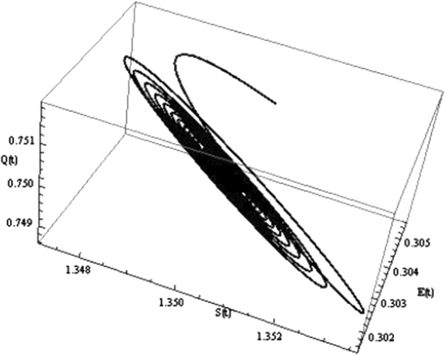
Three-dimensional phase portraits for system (31) for $a=2,b=10,{\beta }_1=0.99,d=0.4,{\beta }_2=0.01,{\beta }_3=0.80,{\beta }_4=0.60,c_1=1,c_2=2$ , $B>0,\mu >0$ and $S_0=1.35,E_0=0.31,Q_0=0.75$

Fig. 10.

Two-dimensional plots and phase portraits for system (31) for $a=2,b=10,{\beta }_1=0.99,d=0.4,{\beta }_2=0.01,{\beta }_3=0.80,{\beta }_4=0.60,c_1=1,c_2=2$ , $B>0,\mu >0$ and $S_0=1.35,E_0=0.31,Q_0=0.75$

Concluding remarks

We study the qualitative behavior of a discrete-time mathematical model for the population suffering from hypertension or diabetes exposed to COVID-19. The continuous-time counterpart of our model was modeled and analyzed in [1] with Z-control. In our study, we discretize the model by using piecewise constant arguments and provides a better graphical and theoretical analysis of model. In addition, in this paper, we considered the reported cases from the early stages of pandemic to the number of cases in the start of year 2020 in country India [1]. Firstly, by assuming the condition that exposed population(E) will remain finite, the boundedness of every positive solution of system (4) is discussed and an explicit lemma for the boundedness of every positive solution of system (4) is provided in Sect. 2. It is shown that there exist six equilibria for system (4). The stability of system (4) is discussed about each of its equilibrium point. Additionally, we have evaluated some mathematical results concerned to existence of one and only positive equilibrium point and some conditions are developed for local asymptotic stability of positive equilibrium point. It is shown that in the absence of quarantined compartment, the system (4) undergoes period-doubling bifurcation and chaos (see Sect. 9). In order to show the complexity in system (4), the existence of Neimark–Sacker bifurcation for one and only positive equilibrium point is proved mathematically. Through numerical study, we show that system (4) undergoes Neimark–Sacker for wide range of bifurcation parameter $\mu .$ Moreover, it is shown that for discrete-time mathematical system (4) and its continuous counterpart (1), if we take death parameter $\mu \le 1$, then both systems are stable and for $\mu >1$ these systems are unstable. A stability comparison of continuous-time mathematical (1) system with its discrete counterpart (4) for death parameter $\mu$ is given in Examples 8.1 and 8.6. It is easy to see that our discrete-time mathematical system undergoes chaos when an individual exposed to COVID-19 does not quarantined himself, that is, for $Q_n\to 0,\forall n,$ the system (4) must be chaotic but for system (1) if $Q(t)\to 0$, then system (1) reduces to a two-dimensional continuous-time system, in which chaos is ceased to exist (see [38, 39]). Thus, our discrete-time mathematical system (4) will remain bounded whenever E is finite and (4) become unbounded when E is unbounded. In addition, an individual which is exposed to COVID-19 must have to quarantine himself such that the system (4) remains stable.

Data Availability Statement

This manuscript has no associated data.

References

- 1.N.H. Shah, N. Sheoran, E. Jayswal, Z-control on COVID-19-Exposed patients in quarantine.Int. J. Differ. Equ., 2020, 1–16 (2020)
- 2.Q. Li, X. Guan, P. Wu, X. Wang, L. Zhou, Y. Tong, R. Ren, K.S. Leung, E.H. Lau, J.Y. Wong, X. Xing, Early transmission dynamics in Wuhan, China, of novel coronavirus-infected pneumonia. New England J. Med. 382, 1199–1207 (2020) [DOI] [PMC free article] [PubMed]
- 3.M. Batista, Estimation of the final size of the COVID-19 epidemic. MedRxiv (2020)
- 4.L. Peng, W. Yang, D. Zhang, C. Zhuge, L. Hong, Epidemic Analysis of COVID-19 in China by Dynamical Modeling. arXiv preprint arXiv:2002.06563 (2020)
- 5.Sun P, Lu X, Xu C, Sun W, Pan B. Understanding of COVID-19 based on current evidence. J. Med. Virol. 2020;92(6):548–551. doi: 10.1002/jmv.25722. [DOI] [PMC free article] [PubMed] [Google Scholar]
- 6.J.F. Rabajante, Insights from Early Mathematical Models of 2019-NCoV Acute Respiratory Disease (COVID-19) Dynamics. arXiv preprint arXiv:2002.05296 (2020)
- 7.Chinazzi M, Davis JT, Ajelli M, Gioannini C, Litvinova M, Merler S, y Piontti AP, Mu K, Rossi L, Sun K, Viboud C. The effect of travel restrictions on the spread of the 2019 novel coronavirus (COVID-19) outbreak. Science. 2020;368(6489):395–400. doi: 10.1126/science.aba9757. [DOI] [PMC free article] [PubMed] [Google Scholar]
- 8.Kucharski AJ, Russell TW, Diamond C, Liu Y, Edmunds J, Funk S, Eggo RM, Sun F, Jit M, Munday JD, Davies N. Early dynamics of transmission and control of COVID-19: a mathematical modelling study. Lancet Infect. Dis. 2020;20(5):553–558. doi: 10.1016/S1473-3099(20)30144-4. [DOI] [PMC free article] [PubMed] [Google Scholar]
- 9.Tang B, Bragazzi NL, Li Q, Tang S, Xiao Y, Wu J. An updated estimation of the risk of transmission of the novel coronavirus (2019-nCov) Infect. Dis. Model. 2020;5:248–255. doi: 10.1016/j.idm.2020.02.001. [DOI] [PMC free article] [PubMed] [Google Scholar]
- 10.Tang B, Wang X, Li Q, Bragazzi NL, Tang S, Xiao Y, Wu J. Estimation of the transmission risk of the 2019-nCoV and its implication for public health interventions. J. Clinical Med. 2020;9(2):462. doi: 10.3390/jcm9020462. [DOI] [PMC free article] [PubMed] [Google Scholar]
- 11.Khan MA, Atangana A, Alzahrani E. The dynamics of COVID-19 with quarantined and isolation. Adv. Differ. Equ. 2020;2020(1):1–22. doi: 10.1186/s13662-019-2438-0. [DOI] [PMC free article] [PubMed] [Google Scholar]
- 12.Awais M, Alshammari FS, Ullah S, Khan MA, Islam S. Modeling and simulation of the novel coronavirus in Caputo derivative. Results Phys. 2020;19:103588. doi: 10.1016/j.rinp.2020.103588. [DOI] [PMC free article] [PubMed] [Google Scholar]
- 13.Oud MAA, Ali A, Alrabaiah H, Ullah S, Khan MA, Islam S. A fractional order mathematical model for COVID-19 dynamics with quarantine, isolation, and environmental viral load. Adv. Differ. Equ. 2021;2021(1):1–19. doi: 10.1186/s13662-020-03162-2. [DOI] [PMC free article] [PubMed] [Google Scholar]
- 14.Alrabaiah H, Safi MA, DarAssi MH, Al-Hdaibat B, Ullah S, Khan MA, Shah SAA. Optimal control analysis of hepatitis B virus with treatment and vaccination. Results Phys. 2020;19:103599. doi: 10.1016/j.rinp.2020.103599. [DOI] [Google Scholar]
- 15.Nawaz M, Wei J, Sheng J, Khan AU. The controllability of damped fractional differential system with impulses and state delay. Adv. Differ. Equ. 2020;2020(1):1–23. doi: 10.1186/s13662-019-2438-0. [DOI] [PMC free article] [PubMed] [Google Scholar]
- 16.Khan MA, Atangana A. Modeling the dynamics of novel coronavirus (2019-nCov) with fractional derivative. Alexandria Eng. J. 2020;59(4):2379–2389. doi: 10.1016/j.aej.2020.02.033. [DOI] [Google Scholar]
- 17.Kolebaje O, Popoola O, Khan MA, Oyewande O. An epidemiological approach to insurgent population modeling with the Atangana-Baleanu fractional derivative. Chaos, Solitons and Fractals. 2020;139:109970. doi: 10.1016/j.chaos.2020.109970. [DOI] [Google Scholar]
- 18.Samanta S. Study of an epidemic model with Z-type control. Int. J. Biomath. 2018;11(07):1850084. doi: 10.1142/S1793524518500845. [DOI] [Google Scholar]
- 19.Alzahrani AK, Alshomrani AS, Pal N, Samanta S. Study of an eco-epidemiological model with Z-type control. Chaos, Solitons and Fractals. 2018;113:197–208. doi: 10.1016/j.chaos.2018.06.012. [DOI] [Google Scholar]
- 20.Singh H, Dhar J, Bhatti HS. Discrete-time bifurcation behavior of a prey-predator system with generalized predator. Adv. Differ. Equ. 2015;2015(1):1–15. doi: 10.1186/s13662-015-0546-z. [DOI] [Google Scholar]
- 21.Kartal S. Dynamics of a plant-herbivore model with differential-difference equations. Cogent Math. 2016;3(1):1136198. doi: 10.1080/23311835.2015.1136198. [DOI] [Google Scholar]
- 22.Khan MS. Stability, bifurcation and chaos control in a discrete-time prey-predator model with Holling type-II response. Network Biol. 2019;9(3):58. [Google Scholar]
- 23.Yang X. Uniform persistence and periodic solutions for a discrete predator-prey system with delays. J. Math. Anal. Appl. 2006;316(1):161–177. doi: 10.1016/j.jmaa.2005.04.036. [DOI] [Google Scholar]
- 24.D.R. Curtiss, Recent extentions of Descartes rule of signs. Ann. Math. 251278, 1–12 (1918)
- 25.Q. Din, A.A. Elsadany, H. Khalil, Neimark-Sacker bifurcation and chaos control in a fractional-order plant-herbivore model. Discrete Dyn. Nature Soc. 2017, 1–12 (2017)
- 26.Din Q. Controlling chaos in a discrete-time prey-predator model with Allee effects. Int. J. Dyn. Control. 2018;6(2):858–872. doi: 10.1007/s40435-017-0347-1. [DOI] [Google Scholar]
- 27.Luo XS, Chen G, Wang BH, Fang JQ. Hybrid control of period-doubling bifurcation and chaos in discrete nonlinear dynamical systems. Chaos, Solitons and Fractals. 2003;18(4):775–783. doi: 10.1016/S0960-0779(03)00028-6. [DOI] [Google Scholar]
- 28.Din Q. Bifurcation analysis and chaos control in discrete-time glycolysis models. J. Math. Chem. 2018;56(3):904–931. doi: 10.1007/s10910-017-0839-4. [DOI] [Google Scholar]
- 29.Din Q, Donchev T, Kolev D. Stability, bifurcation analysis and chaos control in chlorine dioxide-iodine-malonic acid reaction. MATCH Commun. Math. Comput. Chem. 2018;79(3):577–606. [Google Scholar]
- 30.M.S. Shabbir, Q. Din, M. Safeer, M.A. Khan, K. Ahmad. A dynamically consistent nonstandard finite difference scheme for a predator-prey model. Adv. Differ. Equn. 2019(1), 1–17 (2019)
- 31.Din Q. Global stability and Neimark-Sacker bifurcation of a host-parasitoid model. Int. J. Syst. Sci. 2017;48(6):1194–1202. doi: 10.1080/00207721.2016.1244308. [DOI] [Google Scholar]
- 32.Din Q. Global stability of Beddington model. Qual. Theory Dyn. Syst. 2017;16(2):391–415. doi: 10.1007/s12346-016-0197-9. [DOI] [Google Scholar]
- 33.Din Q. Global behavior of a plant-herbivore model. Adv. Differ. Equ. 2015;2015(1):1–12. doi: 10.1186/s13662-015-0458-y. [DOI] [Google Scholar]
- 34.Guckenheimer J, Holmes P. Nonlinear Oscillations, Dynamical Systems, and Bifurcations of Vector Fields. Berlin: Springer; 2013. [Google Scholar]
- 35.Wen G. Criterion to identify Hopf bifurcations in maps of arbitrary dimension. Phys. Rev. E. 2005;72(2):026201. doi: 10.1103/PhysRevE.72.026201. [DOI] [PubMed] [Google Scholar]
- 36.E. Ott, C. Grebogi, J.A. Yorke, Erratum: “Controlling chaos”[Phys. Rev. Lett. 64, 1196 (1990)]. Phys. Rev. Lett. 64(23), 2837 (1990) [DOI] [PubMed]
- 37.Parthasarathy S. Homoclinic bifurcation sets of the parametrically driven Duffing oscillator. Phys. Rev. A. 1992;46(4):2147. doi: 10.1103/PhysRevA.46.2147. [DOI] [PubMed] [Google Scholar]
- 38.Liu X, Xiao D. Complex dynamic behaviors of a discrete-time predator-prey system. Chaos, Solitons and Fractals. 2007;32(1):80–94. doi: 10.1016/j.chaos.2005.10.081. [DOI] [Google Scholar]
- 39.Strogatz S, Friedman M, Mallinckrodt AJ, McKay S. Nonlinear dynamics and chaos: with applications to physics, biology, chemistry, and engineering. Comput. Phys. 1994;8(5):532–532. doi: 10.1063/1.4823332. [DOI] [Google Scholar]
Associated Data
This section collects any data citations, data availability statements, or supplementary materials included in this article.