Methods to evaluate the effectiveness of advanced stop lines for motorcycles in improving road safety

Abstract

In Barcelona, Advanced Stop Lines (ASL) for motorcycles, were implemented since 2009. This paper aims to describe the process followed in determining the best statistical model to analyse the effectiveness of ASL in preventing road traffic injury collisions. A quasi-experimental design of an evaluation study of an intervention with comparison group was performed.

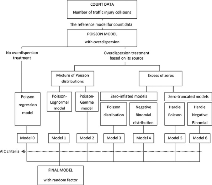
• •The starting model is the Poisson regression model, including type of area (ASL, comparison zone), period (pre and post-intervention), linear trend of the number of collisions, period and type of area interaction, as explanatory variables.
• •Various models are tested to correct existing overdispersion in the starting model: Poisson -Lognormal, Poisson- Gamma, Zero-Inflated Poisson, Zero-Inflated Negative Binomial, Hurdle model with Poisson distribution and with Negative Binomial distribution. To select the best model the Akaike Information Criterion is used. The final model is the Poisson-lognormal, adding the area as random factor (for each area repeated measures for different years are available).
• •The coefficients of the model parameters are interpreted in terms of relatives risks (RR), and the percentage change in the number of collisions is estimated in the post regards the pre-intervention period, from the RRs (- (1-RR)), to quantify the impact of ASL. The interaction allows assessment of whether the effect of the intervention differed between ASL and comparison zones.

Graphical abstract

Specifications table

Subject area:	Medicine and dentistry
More specific subject area:	Public Health
Method name:	Mixed Poisson-lognormal model to evaluate the effectiveness of an intervention with a pre-post study design with comparison group
Name and reference of original method:	[4]. Regression Analysis of Count Data, 2nd edition, Econometric Society MonographNo.53, Cambridge University Press, 1998.
Resource availability	http://faculty.econ.ucdavis.edu/faculty/cameron/racd2/

Introduction

In 2019, a study was published in the Journal of Transport & Health evaluating the effectiveness assessment of advanced stop lines (ASLs) for motorcycles and mopeds in preventing road traffic injury collisions after their implementation in Barcelona in 2009–2010 [17]. To facilitate traffic flow of 2-wheeled motor vehicles, 35 crosswalks were adapted in 2009 to include these ASLs, and another 16 areas were adapted between 2010 and 2011. An ASL is a 4-meter grid painted immediately before the crosswalk, with vertical signalling, so that two-wheeled vehicles wait at the stop lights in front of the cars. This innovative measure had only been previously used for bicycle mobility.

To assess the effectiveness of ASLs, the number of road traffic injury collisions at the adapted crosswalks is evaluated. The number of traffic collisions is a count variable that is discrete, non-negative, and for which a value of 0 is quite frequent. The Poisson regression model is the reference for studying count variables [4], and is particularly appropriate for modelling non-negative integer numbers, especially when the occurrence is low, as is the case of traffic collisions. Using Poisson regression analysis for modelling the number of traffic collisions is problematic due to the lack of compliance with the suppositions of a Poisson distribution. Traffic collisions are not independent phenomena, since the same individual could be involved in more than one collision. In addition, the probability of collision is not the same for all individuals, and having had a collision modifies the probability of having subsequent ones, so these events are neither independent nor constant in time [1,7,10,12,13,16,20]. Given this, the Poisson regression model is expected to have over-dispersion. Overdispersion can be identified when the observed variance exceeds the mean, that is, the observed variance is greater than the theoretical one, since the mean and the theoretical variance are the same in the Poisson distribution. Overdispersion does not invalidate point estimates; these are robust and not biased, if the model is correctly specified. However, these estimates are inefficient, resulting in the real variance being underestimated [7,10,13,20] and, thus, in an extremely narrow confidence interval estimated [7]. This translates into a tendency of the model to make type I error (rejection the null hypothesis when true).

Given these challenges, the aim of this paper is to describe the process that we followed in determining the best statistical model to analyse the effect of ASLs for motorcycles and mopeds implemented in 2009 in Barcelona on road traffic injury collisions, studying the period 2002–2014.

Method details

Departure model

It is based on the Poisson regression model and has the following equation:

$$\log \left(Y\right)=\log \left(\mathrm{E}\left(\mathrm{Y}|\mathrm{X}\right)\right)=XB={\beta }_0+\sum _{j=1}^p\left(x_{ij}{\beta }_j\right)+{\epsilon }_i,wherei=1,\dots ,nandj=1,\dots ,p$$

$$\text{where}\{\begin{array}{c}{\mathrm{y}}_{\mathrm{i}},\text{number}\text{of}\text{road}\text{traffic}\text{injury}\text{collisions}\sim \text{Poisson}\left(\mu \right)\hfill \\ \\ {\mathrm{x}}_{\mathrm{j}},\text{explanatory}\text{variables}\hfill \\ \\ {\beta }_{\mathrm{j}},\text{regression}\text{coefficients}\hfill \\ \\ {\beta }_0,\text{log}\left(\text{probability}\text{of}\mathrm{a}\text{collision}\text{in}\mathrm{a}\text{unit}\text{size}\text{interval}\right),\text{when}\text{all}\text{the}\text{covariables}\text{are}\text{zero}\hfill \\ \\ {\epsilon }_{\mathrm{i}},\text{error}\text{term}\hfill \\ \\ \mathrm{E}\left(\mathrm{Y}|\mathrm{X}\right)=\text{Var}\left(\mathrm{Y}|\mathrm{X}\right)\hfill \end{array}$$

Treatment of overdispersion

We explored all possible models that would allow correcting over-dispersion, based on its source:

A. Over-dispersion may be indicating that the number of traffic collisions is distributed following a mixture of Poisson distributions, such as the Poisson-lognormal [2], [6], [21] or the Poisson-gamma (Negative binomial) [1], [4], [13], [15] distributions.

The Poisson-lognormal regression model allows for overdispersion and a general correlation structure. Starting from a variable Y ~ Poisson (µ),

$${\mu }_{\mathit{ij}}=\exp (x_i{\beta }_j+b_{\mathit{ij}})\mathit{where}{y}_{\mathit{ij}}|b_i,{\beta }_j\sim \mathit{Pois}\mathit{son}\left({\mu }_{\mathit{ij}}\right),b_i|\Sigma \sim \mathit{Norma}{l}_j(0,\Sigma )$$

$$\text{where}\{\begin{array}{c}\mathrm{i}=1,\dots ,\mathrm{n};\mathrm{j}=1,\dots ,\mathrm{p}\hfill \\ \\ \Sigma :\text{Matrix}\text{of}\text{covariances}\hfill \\ \\ \text{Var}\left({\mathrm{y}}_{\text{ij}}\right)>\mathrm{E}\left({\mathrm{y}}_{\text{ij}}\right),\text{allowing}\text{overdispersion}\hfill \end{array}$$

The Negative binomial regression model (Poisson-gamma) is the most widely used in the field of road safety when modelling the number of collisions when there is over-dispersion. In this model, we consider that Y has Poisson distribution, with a mean incompletely specified due to unobserved heterogeneity; this mean is considered a random variable that follows a Gamma distribution in the population. In this case, E (Y | X) is no longer µ = exp (xiβ) but is a random variable,

$$\tilde{\mu }=\exp \left(x_i\beta +{\epsilon }_i\right)=\exp \left(x_i\beta \right)+\exp \left({\epsilon }_i\right)={\mu }_i{\delta }_i$$

where δ_i ~ Gamma (ʋ)

In this way, the equation of the Negative binomial regression model and Poisson regression are the same but, in this case, E (Y | X) = Var (Y | X) is no longer fulfilled.

$$\mathit{Var}\left(y_i|x\right)={\mu }_i(1+\frac{{\mu }_i}{{\nu }_i})=\exp \left(x_i\beta \right)(1+\frac{\exp \left(x_i\beta \right)}{{\nu }_i})$$

B. Another source of over-dispersion could be an excess of zeros, as is common in traffic collisions, given that it is a low occurrence event. In these cases, the most commonly used models are zero-inflated or zero-truncated models.

Zero-inflated regression models model a count variable with an excess of zeros per unit of time. These models assume that there are two processes for generating zeros. The first process is governed by a Binary distribution that generates structural zeros. The second process is governed by a Poisson or Negative binomial distribution that generates counts, some of which can be zero. The global probability of zero counting is the combined probability of zeros in the two processes.

The zero-inflated poisson regression model is as follows [3,5,9,11,15,21]:

$$\begin{array}{ccc}& & P(Y_i=0)={\pi }_i+(1-{\pi }_i)e^{-{\mu }_i}\hfill \\ & & P(Y_i=y_i)=(1-{\pi }_i)\frac{{\mu }^{y_i}{e}^{-{\mu }_i}}{y_i!},y_i\ge 1\hfill \end{array}$$

$$\text{where}\{\begin{array}{c}{\mathrm{Y}}_{\mathrm{i}}=0,\text{in}\text{probability}{\Pi }_{\mathrm{i}}\hfill \\ \\ {\mathrm{Y}}_{\mathrm{i}}\sim \text{Poisson}\left({\mu }_{\mathrm{i}}\right),\text{in}\text{probability}\left(1-{\Pi }_{\mathrm{i}}\right)\hfill \\ \\ \mathrm{E}\left({\mathrm{y}}_{\mathrm{i}}\right)=\left(1-{\Pi }_{\mathrm{i}}\right){\mu }_{\mathrm{i}}\hfill \\ \\ \text{Var}\left({\mathrm{y}}_{\mathrm{i}}\right)={\mu }_{\mathrm{i}}\left(1-{\Pi }_{\mathrm{i}}\right)\left(1+{\mu }_{\mathrm{i}}{\Pi }_{\mathrm{i}}\right)\hfill \end{array}$$

The zero-inflated negative binomial regression model is as follows [8,9,15]:

$$\begin{array}{ccc}& & \mathrm{P}(Y_i=0)={\pi }_i+(1-{\pi }_i){(1+{\mathrm{\alpha }\mu }_{\mathrm{i}})}^{\frac{-1}{\mathrm{\alpha }}}\hfill \\ & & \mathrm{P}(Y_i=y_i)=(1-{\pi }_i)\frac{\Gamma (y_i+\frac{1}{\alpha })}{\Gamma (y_i+1)\Gamma \left(\frac{1}{\alpha }\right)}\frac{{\left(\alpha {\mu }_i\right)}^{y_i}}{{(1+\alpha {\mu }_i)}^{y_i+\frac{1}{\alpha }}},y_i\ge 1\hfill \end{array}$$

$$\text{where}\{\begin{array}{c}{\mathrm{Y}}_{\mathrm{i}}=0,\text{in}\text{probability}{\Pi }_{\mathrm{i}}\hfill \\ \\ {\mathrm{Y}}_{\mathrm{i}}\sim \text{Negative}\text{Binomial}\left({\mu }_{\mathrm{i}},\alpha \right),\text{in}\text{probability}\left(1-{\Pi }_{\mathrm{i}}\right)\hfill \\ \\ \mathrm{E}\left({\mathrm{Y}}_{\mathrm{i}}\right)=\left(1-{\Pi }_{\mathrm{i}}\right){\mu }_{\mathrm{i}}\hfill \\ \\ \text{Var}\left({\mathrm{Y}}_{\mathrm{i}}\right)={\mu }_{\mathrm{i}}\left(1-{\Pi }_{\mathrm{i}}\right)\left(1+{\mu }_{\mathrm{i}}\left({\Pi }_{\mathrm{i}}+\alpha \right)\right)\hfill \end{array}$$

Regarding zero-truncated models, the most commonly used is the hurdle two-step model. This is also a two-component model, in which one component models the probability of zero counts (binary decision model generated by an f1 distribution) and the other component uses a truncated distribution under the condition of a positive result (model truncated in zero generated by a f2 distribution, which will be a binomial negative or Poisson). The hurdle model considers zeros to be completely independent of non-zeros, and is represented as follows [14]:

$$\begin{array}{ccc}& & \mathrm{P}(Y_i=0)=f1\left(0\right)\hfill \\ & & \mathrm{P}(Y_i=y_i)=1-f1\left(0\right))\frac{f2\left(y_i\right)}{1-f2\left(0\right)},y_i\ge 1\hfill \end{array}$$

$$\text{where}\{\begin{array}{c}1-\mathrm{f}1\left(0\right):\text{probability}\text{of}\text{getting}\mathrm{a}\text{value}>0\hfill \\ \\ \frac{f2\left(y_i\right)}{1-f2\left(0\right)}:\text{probability}\text{of}\text{obtaining}\mathrm{a}\text{value}\text{yi},\text{knowing}\text{that}\text{the}\text{value}\text{obtained}\text{is}>0\hfill \end{array}$$

Method validation

A. Validation strategy

We started first with a Poisson regression model, evaluated overdispersion and, if present, treated overdispersion with the models presented in the previous section. We validated the best model using the data from the effectiveness assessment analysis of ASLs for motorcycles and mopeds in preventing road traffic injury collisions, described in the original article published in 2019 [17], and the Poisson regression model used was based on the methodology described in it, using only part of the data: those of the 35 ASLs implemented in 2009 (phase I), which refer to the CROSS study area (crosswalk and subsequent intersection). In addition, of all the outcome variables used in the evaluation study (total number of collisions, people injured, collisions involving a motorcycle, and motorcycle drivers involved), only the number of collisions were used in validating the model. Explanatory variables were the following:

• •Year: from 2002 to 2014.
• •Period: Pre-intervention (2002-2009) and post-intervention (2010-2014).
• •Type of zone (Type_zone): ASL, comparison (Non-ASL).
• •
  Street characteristics:

  • ○
    Average daily traffic (ADT), which is a measure of the traffic volume of motor vehicles.
  • ○
    Carriageway width (Width)
  • ○
    Number of traffic lanes (N_lanes)
  • ○
    Number of service streets with street furniture, parking spaces, etc. (N_service)
  • ○
    Number of bus lanes (N_bus)
• •
  Collision characteristics:

  • ○
    Type of collision: run-over, head-on, side-impact, front-side impact, rear-end, crash against a static element, overturning (four-wheeled vehicles), falls (two-wheeled vehicles), and falls inside a vehicle (bus). All these variables were dichotomous (yes, no).
  • ○
    Motorcycle or moped involvement (yes, no).
  • ○
    Pedestrian involvement (yes, no).
  • ○
    Bicycle involvement (yes, no).
  • ○
    Collision producing a serious or fatal injury (yes, no).

The first model used to analyse the data was the following Poisson regression model (Model0):

$$\text{Ln}\left(\mathrm{Y}\right)\sim \text{Trend}+\text{Period}*\text{Type}\_\text{zone}+\text{ADT}+\mathrm{N}\_\text{service}+\mathrm{N}\_\text{lanes}+\mathrm{N}\_\text{bus}+\text{Width}$$

This model includes the Type_zone, Period, ADT, N_service, N_lanes, N_bus Width, and Trend variables. The Trend variable gathers the linear trend and includes an interaction between Period and Type_zone (Period*Type_zone), which allows evaluating whether the effect of the intervention (number of collisions in the post-intervention period versus the pre-intervention period) is significantly different in ASL zones than in comparison zones.

All models were defined with the same structure as Model0, and the Akaike information criterion (AIC) was used to estimate the relative quality of a statistical model to select the most appropriate one. The AIC measures the goodness-of-fit and complexity, and offers a relative estimate of the amount of information lost when using a particular model to represent the process that generates the data. Generally speaking, the AIC index equals 2K-2ln (L), where K is the model parameter number and L is the maximum value of the likelihood function for the estimated model. The model with the lowest AIC, among those that correct for over-dispersion, is considered the best model. There are other criteria that are also widely used in these cases, such as the BIC (Bayesian Information Criterion). But we chose the AIC instead of the BIC because AIC is better in situations when a false negative finding would be considered more misleading than a false positive, and BIC is better in situations where a false positive is as misleading as, or more misleading than, a false negative. A false negative could mean not detecting an increase in the number of collisions. As we are evaluating an intervention in road safety, we are especially interested in detecting the increase in cases to decide whether to continue implementing the intervention or not or withdraw it, to protect people's health.

The area was added as a random factor to the final model, since both ASLs and comparison zones had repeated measurements of traffic collisions occurring year by year from 2002 to 2014. The random factor was added after the model selection process so that the AIC of the models were comparable.

B. Validation of results

Table 1 shows all the models that were adjusted, their R language formulation and AIC values.

Table 1.

Models adjusted in order to correct overdispersion, with their R language formulation and AIC values.

Model name	R language formulation	AIC value
Model0	glm(Collisions ~ trend+Period*Type_zone+ADT+N_lanes+Width+N_service+N_bus,ASLCROSS,family=poisson)	4,558.00
Model1	glmer(Collisions ~ trend+Period*Type_zone+ADT+N_lanes+Width+N_service+N_bus+(1|ASLCROSS$obs),ASLCROSS,family=poisson)	4,073.50
Model2	glm.nb(Collisions ~ trend+Period*Type_zone+ADT+N_lanes+Width+N_service+N_bus,ASLCROSS)	4,073.00
Model3	glmmadmb(Collisions ~ trend+Period*Type_zone+ADT+N_lanes+Width+N_service+N_bus,data=ASLCROSS,zeroInflation=TRUE,family="poisson")	4,460.92
Model4	glmmadmb(Collisions ~ trend+Period*Type_zone+ADT+N_lanes+Width+N_service+N_bus,data=ASLCROSS,zeroInflation=TRUE,family="nbinom")	4,075.04
Model5	hurdle(Collisions ~ trend+Period*Type_zone+ADT+N_lanes+Width+N_service+N_bus, dist = "negbin", data = ASLCROSS)	4,064.15
Model6	hurdle(Collisions ~ trend+Period*Type_zone+ADT+N_lanes+Width+N_service+N_bus, dist = "poisson", data = ASLCROSS)	4,427.49

The average annual number of collisions per area in the CROSS study areas, from 2002 to 2014, was less than the variance in both ASL and comparison zones (average of 4.8 and 3.4, and variance of 21.6 and 15.2, respectively). Therefore, it was confirmed that the initial model (Model0), which is a Poisson regression, had overdispersion. Fig. 1 shows the dispersion of the values adjusted by Model0 and overdispersion can be observed, since the dispersion increases.

Fig. 1.

Scatter of the values adjusted by the initial model, Model0 (mod0).

Model1 (Poisson-lognormal model) consisted on adding a random effect that collected the variability between each observation to the initial model (Model0). Model1 was used both to determine the existence of overdispersion and to correct it. Table 1 shows that the AIC in Model 1 is greatly reduced compared to Model0 from 4,558 to 4,073.5, therefore confirming the overdispersion of the initial model and indicating Model1 is better, since it corrected it (coefficient of overdispersion, 1.06). Fig. 2 shows how Model1 did not exhibit overdispersion.

Fig. 2.

Scatter of the values adjusted by Model1.

Model2 (Negative binomial model or Poisson-gamma model), Model4 (Zero-inflated negative binomial model) and Model5 (Hurdle model with negative binomial distribution) presented AIC values very similar to Model1 (Table 1) and were also better models than the initial one (Model0) but continued to show overdispersion, as shown in Fig. 3, Fig. 4, Fig. 5.

Fig. 3.

Scatter of the values adjusted by Model2.

Fig. 4.

Scatter of the values adjusted by Model4.

Fig. 5.

Scatter of the values adjusted by Model5.

Model3 (Zero-inflated poisson model) and Model6 (Hurdle model with poisson distribution) also had lower AIC than that of the initial model but higher than that of Models 1, 2, 4 and 5.

Therefore, it was determined that the best model for analysing this type of data was Model1, the Poisson-lognormal model, because it had one of the lowest AICs and did not have overdispersion.

C. Final model

By entering the area as a random factor in Model1 (ModelFinal), the AIC was reduced from 4,073.5 to 3,662.2, and the Chi-square test to compare the models (i.e. it tests whether reduction in the residual sum of squares are statistically significant) was significant (p<0.001).

The results of the comparison of Model1 and ModelFinal using the Chi-square test from the ANOVA function in R-software, and the results of the final model (ModelFinal), can be found in Supplementary material section.

A graphical analysis of the residuals was performed to validate the final model (ModelFinal) and we concluded that it was valid and without overdispersion (Fig. 6). The graphs used were the following: A. Quantile graph of the residuals in order to evaluate their normality; B. Quantile graph of the random effects in order to evaluate their normality; C. Graph of standardized residuals versus adjusted values to check the homogeneity of variance of residuals; D. Dispersion graph between observed and expected values, in order to evaluate overdispersion.

Fig. 6.

Final model (ModelFinal) validation graphs.

The coefficients of the model parameters are interpreted in terms of relatives risks (RR), which are the exponential coefficients. From the RR the percentage change in the number of road traffic collisions is estimated in the post-intervention period regards the pre-intervention period (% change = (- (1-RR))), to quantify the impact of the implementation of ASL.

Analyses were carried out with software STATA version 13.0 [19] and R version 3.2.1 (R [18]).

Conclusion

The Poisson Lognormal regression model is a good alternative to the Negative Binomial (Poisson-Gamma) regression model when modelling the number of collisions with the presence of over-dispersion. The Poisson Lognormal model allows not only over-dispersion but also a general correlation structure. This model has turned out to be the best model among the main alternative models to correct for over-scattering based on its source.

Declaration of Competing Interest

The authors declare that they have no known competing financial interests or personal relationships that could have appeared to influence the work reported in this paper.

References

- 1.Abdel-Aty M.A., Radwan E.A. Modeling traffic accident occurrence and involvement. Accid. Anal. Prev. 2000;32:633–642. doi: 10.1016/s0001-4575(99)00094-9. [DOI] [PubMed] [Google Scholar]
- 2.Aitchison J., Ho CH. The multivariate Poisson-Log Nomal distribution. Biometrika. 1989;4(76):643–653. [Google Scholar]
- 3.Böhning D., Dietz E., Schlattmann P., Mendoca L., Kirchner U. The zeroinflated Poisson model and the decayed, missing and filled teeth index in dental epidemiology. J. R. Stat. Soc. Ser. A. 1999;162:195–209. [Google Scholar]
- 4.Cameron A.C., Trivedi P.K. 2nd Ed. Vol. 1998. Cambridge University Press; 2013. Regression analysis of count data. (Econometric Society Monograph No.53). [Google Scholar]
- 5.Cheung Y.B. Zero-inflated models for regression analysis of count data: a study of growth and development. Stat. Med. 2002;21:1461–1469. doi: 10.1002/sim.1088. [DOI] [PubMed] [Google Scholar]
- 6.Elston D.A., Moss R., Bouliner T., Arrowsmith C., Lambin X. Analysis of aggregation, a worked exemple: number of ticks on red grouse. Parasitology. 2001;122:563–569. doi: 10.1017/s0031182001007740. [DOI] [PubMed] [Google Scholar]
- 7.Glynn R.J., Stukel T.A., Sharp S.M., Bubolz T.A., Freeman J.L., Fisher E.S. Estimating the variance of standarized rates of re- current events, with application to hospitalizations among the elderly in New England. Am. J. Epidemiol. 1993;7:776–786. doi: 10.1093/oxfordjournals.aje.a116738. [DOI] [PubMed] [Google Scholar]
- 8.Greene W.H. Department of Economics, Stern School of Business. New York University; New York: 1994. Accounting for excess zeros and sample selection in Poisson and negative binomial regression models. working paper. [Google Scholar]
- 9.Lambert D. Zero-inflated Poisson regression with an application to defects in manufacturing. Technometrics. 1992;34:1–14. [Google Scholar]
- 10.Lawless J.F. Negative binomial and mixed Poisson regression. Can. J. Stat. 1987;15:209–225. [Google Scholar]
- 11.Lee A.H., Wang K., Yau K.K.W. Analysis of zero-inflated Poisson data incorporating extent of exposure. Biom. J. 2001;43:963–975. [Google Scholar]
- 12.Lindsey J.K. Ox- ford University Press; Oxford: 1994. Models for Repeated Measuraments. [Google Scholar]
- 13.Miaou S.P. The relationship between truck accidents and ge- ometric design of road sections: Poisson versus negative bi- nomial regressions. Accid. Anal. Prev. 1994;26:471–482. doi: 10.1016/0001-4575(94)90038-8. [DOI] [PubMed] [Google Scholar]
- 14.Mullahy J. Specification and testing of some modified count data models. J. Econom. 1986;33:341–365. [Google Scholar]
- 15.Nakashima E. Some methods for estimation in a Negative-Binomial model. Ann. Inst. Statist. Math. 1997;49:101–105. [Google Scholar]
- 16.Navarro A., Utzet F., Puig P., Caminal J., Martin M. La distribución binomial negativa frente a la de Poisson en el anàlisis de fenómenos recurrentes. Gac. Sanit. 2001;15:447–452. doi: 10.1016/s0213-9111(01)71599-3. [DOI] [PubMed] [Google Scholar]
- 17.Perez K., Santamariña-Rubio E. Do advanced stop lines for motorcycles improve road safety? J. Transp. Health. 2019;15 [Google Scholar]
- 18.Core Team R. R Foundation for Statistical Computing; Vienna, Austria: 2015. R: A Language and Environment for Statistical Computing.https://www.R-project.org/) URL. [Google Scholar]
- 19.StataCorp. StataCorp LP; TX: 2013. Stata Statistical Software: Release 13. College Station. [Google Scholar]
- 20.Venables W.N., Ripley B.D. 2nd Ed. Springer-Verlag; Nueva York: 1997. Modern Applied Statistics with S-Plus. [Google Scholar]
- 21.Vives Brosa J. Doctoral thesis directed by Doctor Losilla Vidal J.M. Universitat Autònoma de Barcelona. Facultat de psicologia. Departament de psicologia i de metodologia de les ciències de la salut; 2002. El diagnóstico de la sobredispersión en modelos de análisis de datos de recuento.http://hdl.handle.net/10803/5422 [Google Scholar]
Associated Data
This section collects any data citations, data availability statements, or supplementary materials included in this article.