Adaptively Learning Local Shape Statistics for Prostate Segmentation in Ultrasound

Abstract

Automatic segmentation of the prostate from 2-D transrectal ultrasound (TRUS) is a highly desired tool in many clinical applications. However, it is a very challenging task, especially for segmenting the base and apex of the prostate due to the large shape variations in those areas compared to the midgland, which leads many existing segmentation methods to fail. To address the problem, this paper presents a novel TRUS video segmentation algorithm using both global population-based and patient-specific local shape statistics as shape constraint. By adaptively learning shape statistics in a local neighborhood during the segmentation process, the algorithm can effectively capture the patient-specific shape statistics and quickly adapt to the local shape changes in the base and apex areas. The learned shape statistics is then used as the shape constraint in a deformable model for TRUS video segmentation. The proposed method can robustly segment the entire gland of the prostate with significantly improved performance in the base and apex regions, compared to other previously reported methods. Our method was evaluated using 19 video sequences obtained from different patients and the average mean absolute distance error was 1.65 ± 0.47 mm.

I. Introduction

Prostate cancer is the second leading cause of cancer death in men in the U.S. [1]. Transrectal ultrasound (TRUS) is currently the most commonly used imaging modality for image-guided biopsy and therapy of prostate cancer due to its real-time nature, low cost, and simplicity. Accurate segmentation of the whole prostate from TRUS can play a key role in biopsy and therapy planning [2], and allow for surface-based registration between TRUS and other imaging modalities (e.g., MRI) during the image-guided intervention [3]. However, segmentation of the prostate from TRUS is a challenging problem due to the inhomogeneous intensity distribution of the prostate and the low SNR of ultrasound. Extraction of the prostate boundary in the base and apex areas is even more difficult because of the large shape variations in those areas.

A number of methods for prostate segmentation in static 2-D TRUS images have been reported in the past decade [4]–[12]. However, poor segmentation performance of the 2-D model-based methods in the base and apex areas of the prostate was also indicated. There are several reasons for that. First of all, boundaries of the prostate in the base and apex can be quite different from patient to patient. More importantly, the prostate shape changes significantly from frame to frame with little movement of the TRUS probe. Thus, a global population-based 2-D shape model is not able to capture the variation effectively for the segmentation. Although 3-D-based methods may have better segmentation performance in the base and apex [13], [14], they have limited use in clinical applications because 3-D TRUS is still in its early stage. Segmentation of the 3-D images reconstructed from 2-D frames is not an option either due to the image blurring and other artifacts caused by ultrasound probe motion and the organ movement [15].

In order to improve the performance of the prostate segmentation in the base and apex areas, we propose adaptively learning the local shape statistics for segmenting the prostate in TRUS video sequences, which usually cover the whole prostate by sweeping the gland with a ultrasound probe as shown in Fig. 1. To the best of our knowledge, this is the first method that addresses the segmentation of the whole prostate gland from 2-D TRUS video sequences [16], [17].

Fig. 1.

Example images of the prostate in the (a) base, (b) midgland, and (c) apex areas, respectively, for the same patient. There are large prostate shape variations between the images.

Dynamic shape priors have been used in previous works for segmenting and tracking the left ventricle in cardiac images [18]–[20]. However, those methods build the dynamic model using predefined training set and the model cannot be updated online as new segmentation results become available. Thus, their applications are limited to segmenting targets under cyclic motion like the heart. Recently, Shi et al. [21] used both population-based and patient-specific shape statistics for segmenting the lung fields in serial chest radiographs. The method has also been applied to segmenting the prostate from series of 3-D CT scans [22]. In their work, the initial several images are segmented with population-based shape statistics. As more segmentation results become available, patient-specific shape statistics are obtained to guide segmentation for better accuracy. However, their method can only deal with segmenting a series of images of a static object, since the dynamic shape changes occurred in a short period of time are smoothed over the whole shape set and not captured.

In this paper, we propose a new TRUS video segmentation framework for segmenting the intersected prostate shape from any part of the gland by using both global population-based shape statistics (GPSS) and adaptive local shape statistics (ALSS). The TRUS video sequences to be segmented in our work were obtained by sweeping the prostate from the base to apex in the axial orientation with an ultrasound probe. Our proposed method starts segmenting the prostate using GPSS. After segmenting enough number of video frames for shape modeling, the local patient-specific shape statistics can be learned and applied to guide the segmentation. Unlike the work in [21] and [22], where the patient-specific shape model is built by using all the available images, the patient-specific shape statistics in our work is adaptively updated to get local shape changes using a relatively small group of frames. In other words, the local shape statistics is continuously recomputed using a set of local training shapes by discarding old shapes. In this way, not only the patient-specific shape statistics but also the shape variations in a local neighborhood can be effectively captured, which provides very good shape prior guidance for the segmentation. Therefore, the whole prostate, especially the base and apex areas, can be successfully segmented from TRUS.

The rest of the paper is organized as follows. The learning of GPSS and ALSS is presented in Section II. The complete TRUS video segmentation framework is provided in Section III. The performance of the proposed method is demonstrated in Section IV with quantitative evaluation on TRUS video sequences. Conclusion is drawn in Section V.

II. Prostate Shape Modeling

The methods for learning the prostate shape statistics are presented in this section. We start shape modeling from GPSS and then extend it to ALSS.

A. Global Population-Based Shape Statistics

GPSS describes the statistics of the shapes covering all the areas of the prostate from a population. Thus, the training shape set is composed by the manually segmented contours from the base to the apex of the prostate in the axial orientation of different subjects. The principal component analysis-based shape modeling method proposed by Cootes et al. [23] is employed in our work for computing GPSS. Each prostate shape S in the training shape set is represented by l 2-D points as the vector

$$S={\left[x_1,x_2,\dots ,x_l;y_1,y_2,\dots ,y_l\right]}^T$$ (1)

which is an observation in the 2l -dimensional space. In our study, the contour points are extracted from the shapes by using equally spaced sampling. In order to establish the correspondence between the contour points from different shapes, the sampling is always performed clockwise and starts from the point where a ray cast from the center of the shape toward left meets the shape. The computed GPSS S_G consists of a mean shape, an eigenshape matrix, and the corresponding eigenvalues. The mean shape is computed as

$${\overline{S}}_G=\frac{1}{L}\sum _{i=1}^L{S}_i$$ (2)

where L is the number of the training shapes. Subtracting the mean shape from each training shape, a (2l × L)-dimensional matrix P can be constructed by considering the resulting shape differences as column vectors. By using singular value decomposition, the matrix is decomposed as

$$\mathbf{P}=\mathbf{U}\mathbf{\Sigma }\mathbf{V}.$$ (3)

The orthogonal column vectors of the matrix U are the modes of shape variation, i.e., eigenshapes. The diagonal matrix Σ is composed of the corresponding eigenvalues, which are the magnitudes of the shape variations. The modes are ordered according to the percentage of variation that they explain. In our paper, we set the percentage threshold as 98% of the total variation to choose the first k largest modes for a compact representation. GPSS is only computed once in the training phase using all the provided training shapes.

With the computed shape statistics, a new shape S can be decomposed by using the mean shape and the eigenshapes and represented by a parameter vector b as

$$\mathbf{b}={\mathbf{U}}^T\left(S-{\overline{S}}_G\right).$$ (4)

The approximation of the shape constrained by the shape statistics is obtained by

$$\widehat{S}={\overline{S}}_G+\mathbf{Ub}.$$ (5)

Some shape samples generated by using GPSS are shown in Fig. 2.

Fig. 2.

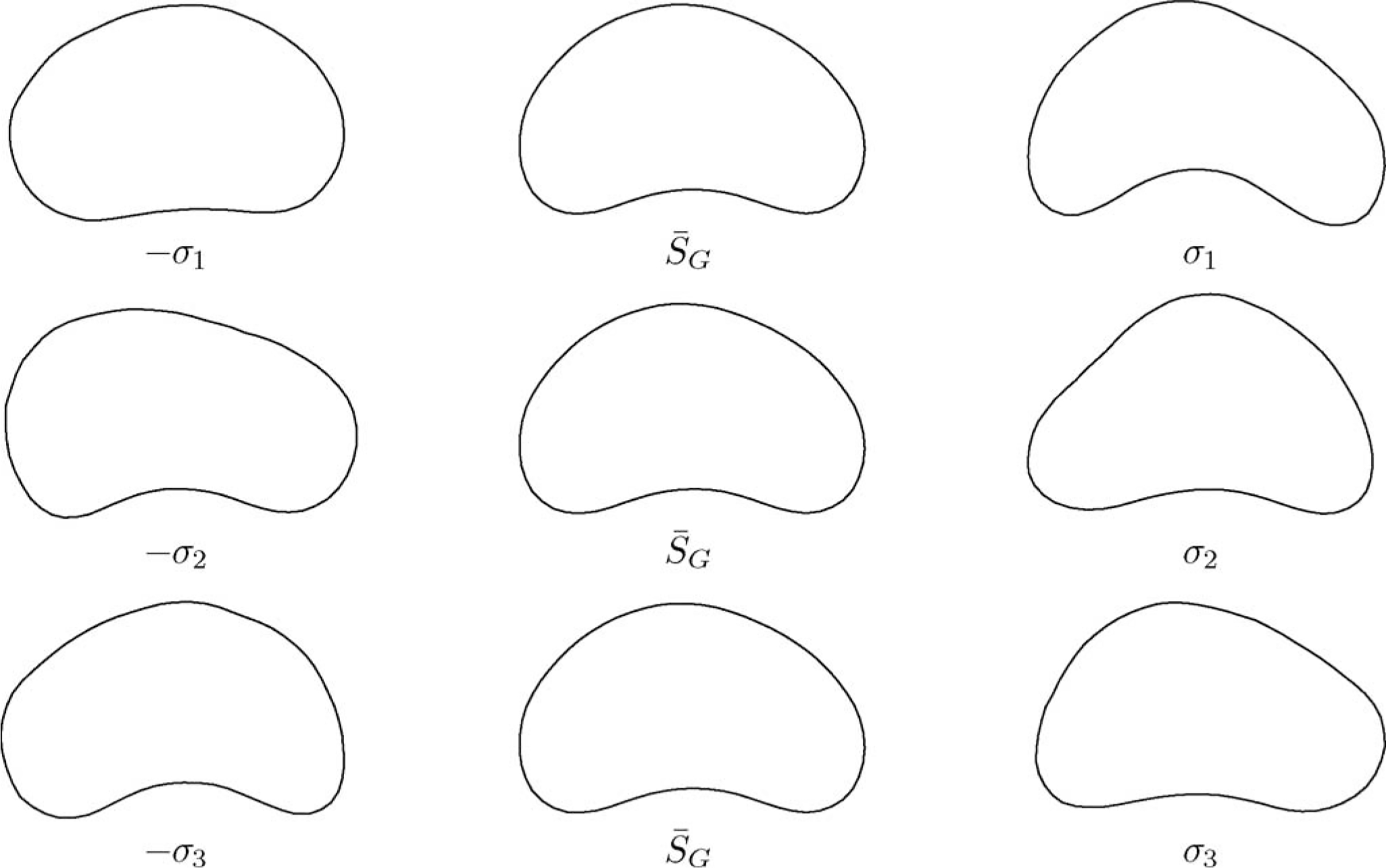
Example shapes generated by the GPSS. The mean shape ${\overline{S}}_G$ is drawn in the second column. Shapes generated by varying the mean shape with the largest three modes of variation (σ₁, σ₂, σ₃) are drawn in the first and third rows, respectively.

B. ALSS

ALSS ${\mathcal{S}}_A^t$ is continuously learned at each time t during the segmentation process, which describes the statistics of the prostate shape in a local area. Each ALSS consists of a mean shape, an eigenshape matrix, and the corresponding eigenvalues. To adaptively capture the shape changes in local neighborhood, ALSS is learned from the N most recent segmented contours {S_i|i = t − N + 1, …, t} of a subject. The mean shape is computed as

$${\overline{S}}_A^t=\frac{1}{N}\sum _{i=t-N+1}^t{S}_i$$ (6)

and the eigenvalues and eigenvectors are computed by

$${\mathbf{P}}^t={\mathbf{U}}^t{\mathbf{\Sigma }}^t{\mathbf{V}}^t.$$ (7)

The computed ALSS instance ${\mathbf{S}}_A^t$ at time t is then used for segmenting the frame at t + 1 with the segmented contour S_t for initialization. Once the segmentation is done, the obtained prostate shape S_t+1 will be added into the training shape set and shape S_t−N+1 will be removed. ALSS is updated using (6) and (7) with the new set of training shapes and denoted as S_t+1. With the updated ALSS, we move to segment the next frame. The learning and segmentation process is repeated until the whole video sequence is segmented. Sample shapes generated by ALSS at different times are shown in Fig. 3.

Fig. 3.

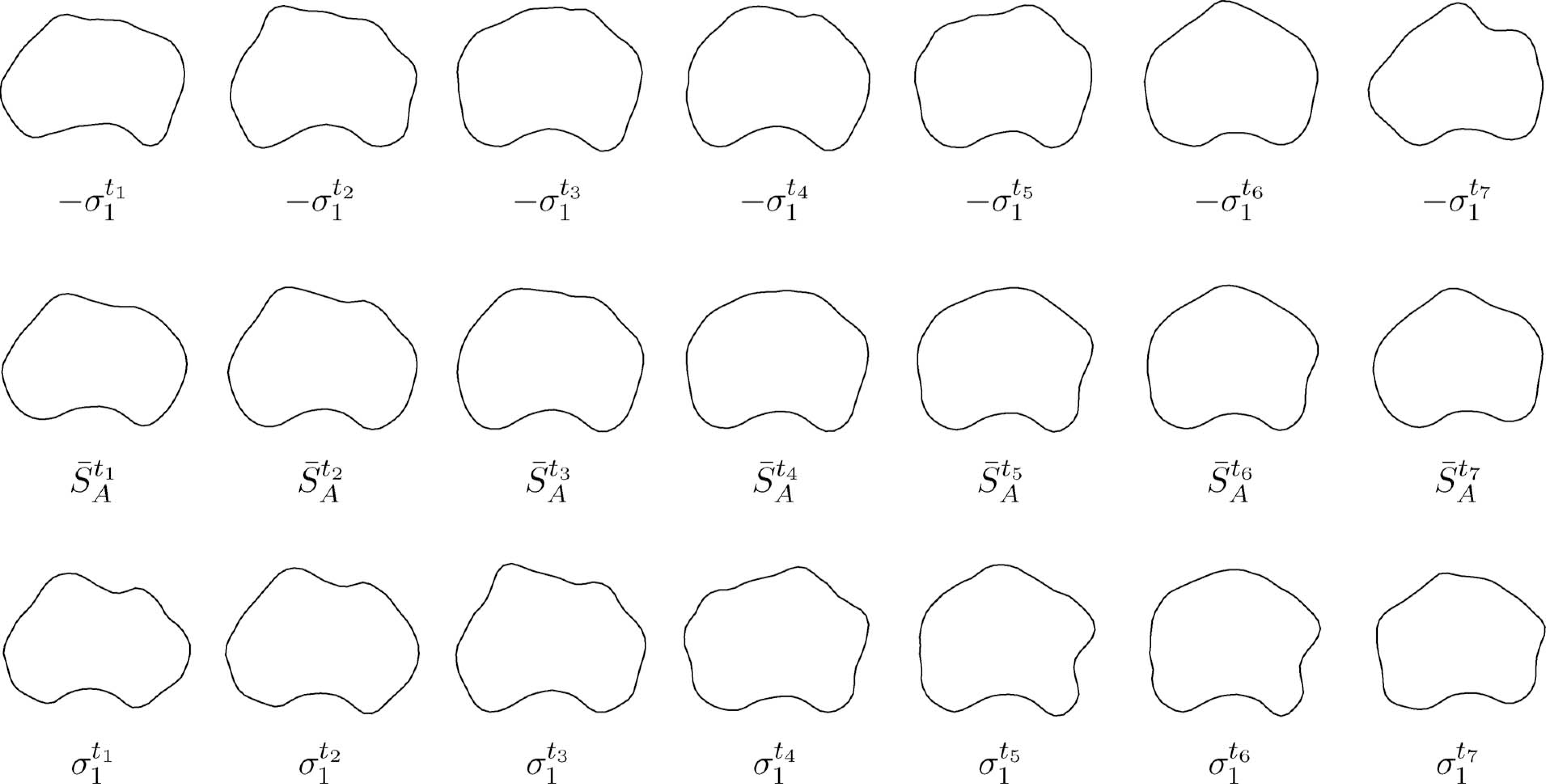
Example shapes generated by the ALSS. The mean shapes ${\overline{S}}_A^t$ at each time instance are drawn in the second row. Shapes generated by varying the mean shapes with the largest mode of variation ${\sigma }_1^t$ at each time are drawn in the first and third rows, respectively.

III. TRUS Video Segmentation

A. Model-Based Segmentation

The GPSS and ALSS are used together with the discrete deformable model (DDM) [4] for prostate segmentation. The DDM consists of a deformable contour S represented by a series of K contour points, i.e., S = {v_i|i = 1, …, K}, and an associated energy functional. The prostate is segmented from TRUS video sequences by deforming the contour to minimize the energy functional in each frame. In our paper, the energy functional of a contour point v_i in DDM for segmenting the video frame at time t is defined as

$$E^t\left({\mathbf{v}}_i\right)=E_{\text{image}}^t\left({\mathbf{v}}_i\right)+E_{\text{int}}^t\left({\mathbf{v}}_i\right)+E_{\text{shape}}^t\left({\mathbf{v}}_i\right).$$ (8)

The image term $E_{\text{imag}e}^t\left({\mathbf{v}}_i\right)$ in (8) attracts the contour toward the prostate boundary by searching for prostate boundary features in the image. The easily observable dark-to-bright transition around the prostate in TRUS images is considered as a discriminative boundary feature [4], [24], which is obtained by computing the contrast of the normal vector profile (NVP) of a candidate contour point

$$E_{\text{imag}e}^t\left({\mathbf{v}}_i\right)=\frac{1}{2m}{\mathbf{p}}^T\cdot {\mathbf{f}}_i.$$ (9)

The contrast filter p is a vector defined as [1, …, 1, −1, …, −1]^T with length 2m, where 2m denotes the total number of points on NVP. Let n denote the normal direction of the contour at point v_i, which is pointing from inside to outside. NVP f_i is a vector [f_i1, f_i2, …, f_i2m]^T, where the element f_ij is the intensity of the jth pixel at location v_ij = v_i + (j − m)δn and δ is a spacing parameter.

The internal energy term $E_{\text{int}}^t\left({\mathbf{v}}_i\right)$ in (8) preserves the geometric shape of the contour during deformation by applying the constraints of continuity and curvature as in [25]. In our study, we consider the case when E_int(v_i) includes the second-order term, i.e., the computation of E_int(v_i) involves the contour points v_i−1 and v_i+1. The internal energy term can be computed as

$$\begin{gathered} E_{\text{int}}\left({\mathbf{v}}_i\right)=\alpha \left(\Vert {\mathbf{v}}_i-{\mathbf{v}}_{i-1}\Vert +\Vert {\mathbf{v}}_{i+1}-{\mathbf{v}}_i\Vert -2d\right) \\ +\beta \Vert \left({\mathbf{v}}_i-{\mathbf{v}}_{i-1}\right)-\left({\mathbf{v}}_{i+1}-{\mathbf{v}}_i\right)\Vert \end{gathered}$$ (10)

where α and β are the weights of the continuity and curvature, respectively, and d is the average distance between neighboring model points. The first term on the right side of (10) tends to keep the contour points from either too close or too far. The second term smooths the model by penalizing sharp angles.

The shape energy term $E_{\text{shape}}^t(\mathbf{v})$ applies the shape constraint derived from a priori shape statistics to the segmented contour. It is defined by the distance between point v_i from the contour and the corresponding point ${\mathbf{v}}_i^{\prime }$ from the shape prior ${\widehat{S}}^t$ estimated by using either GPSS or ALSS

$$E_{\text{shape}}^t\left({\mathbf{v}}_i\right)=\gamma \Vert {\mathbf{v}}_i-{\mathbf{v}}_i^{\prime }\Vert$$ (11)

where γ is a positive weighting parameter. The correspondence between the points is determined by the orders that the contour points are sampled from the shapes as presented in Section II-A.

The shape constraint plays a key role in prostate segmentation, where the essential part is the estimation of the shape prior ${\widehat{S}}^t$. The shape statistics S^t used for segmenting frame t is defined as

$${\mathbf{S}}^t=\{\begin{array}{ll}{\mathbf{S}}_G,\hfill & \text{if}t-t_0<N\hfill \\ {\mathbf{S}}_A^t,\hfill & \text{if}t-t_0\ge N\hfill \end{array}$$ (12)

where t₀ is the starting frame number and N is the number of frames that are used for computing ALSS. The shape statistics definition in (12) indicates that GPSS is used when segmenting the first N frames. After that, ALSS can be initialized using the segmented shapes, which then takes over the shape constraint term. Once available, ALSS will also be updated adaptively during the segmentation process as described earlier.

B. Energy Minimization

A two-step optimization strategy is used to minimize the energy in (8). In the first step, the iterative shape fitting method of the active shape model (ASM) is employed [23]. To quickly deform the shape to get close to the prostate boundary, only the first and the third terms of (8) are used in this step. In each iteration, a deformable contour is first updated via a local search around its current location along the normal directions of the contour for the dark-to-bright transition of prostate boundary. Then shape statistics S^t is used to constrain the newly updated deformable contour according to (12). In our work, three iterations are done in a coarse-to-fine multiresolution fashion. The ASM fitting method is robust but not accurate enough due to the strong shape constraint. However, it can provide a very good starting point for the deformable segmentation in the second step.

In the second step, deformable segmentation is performed. In each iteration of the deformable segmentation, the deformable contour is updated via a local search with all the three terms of the energy function (8) considered simultaneously. Since the internal energy term is second order, i.e., computation of the term requires more than one contour point, a full search for minimization is computationally very expensive. For fast computation, the dynamic programming technique in [26] is used in our study for energy minimization. It guarantees to get the global minimum inside the search range and the computational complexity is only O(nm³), where n is the number of contour points and m is the size of search range.

C. Segmentation Scheme

The overall segmentation scheme of the proposed method is shown in Fig. 4. In our method, GPSS is first computed by using a number of manually segmented contours obtained from a number of different subjects’ TRUS video sequences. The GPSS deformable contour defined in (8) is used to segment the first N frames from frame 0 to frame N − 1 independently. The mean shape ${\overline{S}}_G$ in the GPSS is used to automatically initialize the segmentation contour. The resulting shapes {S_i|i = 0, …, N − 1} will be stored. After that, an initial ALSS, denoted by ${\mathbf{S}}_A^{N-1}$, is computed by using the segmented contours from those N frames. This ALSS is then used as the shape constraint of the deformable contour for segmenting the next frame.

Fig. 4.

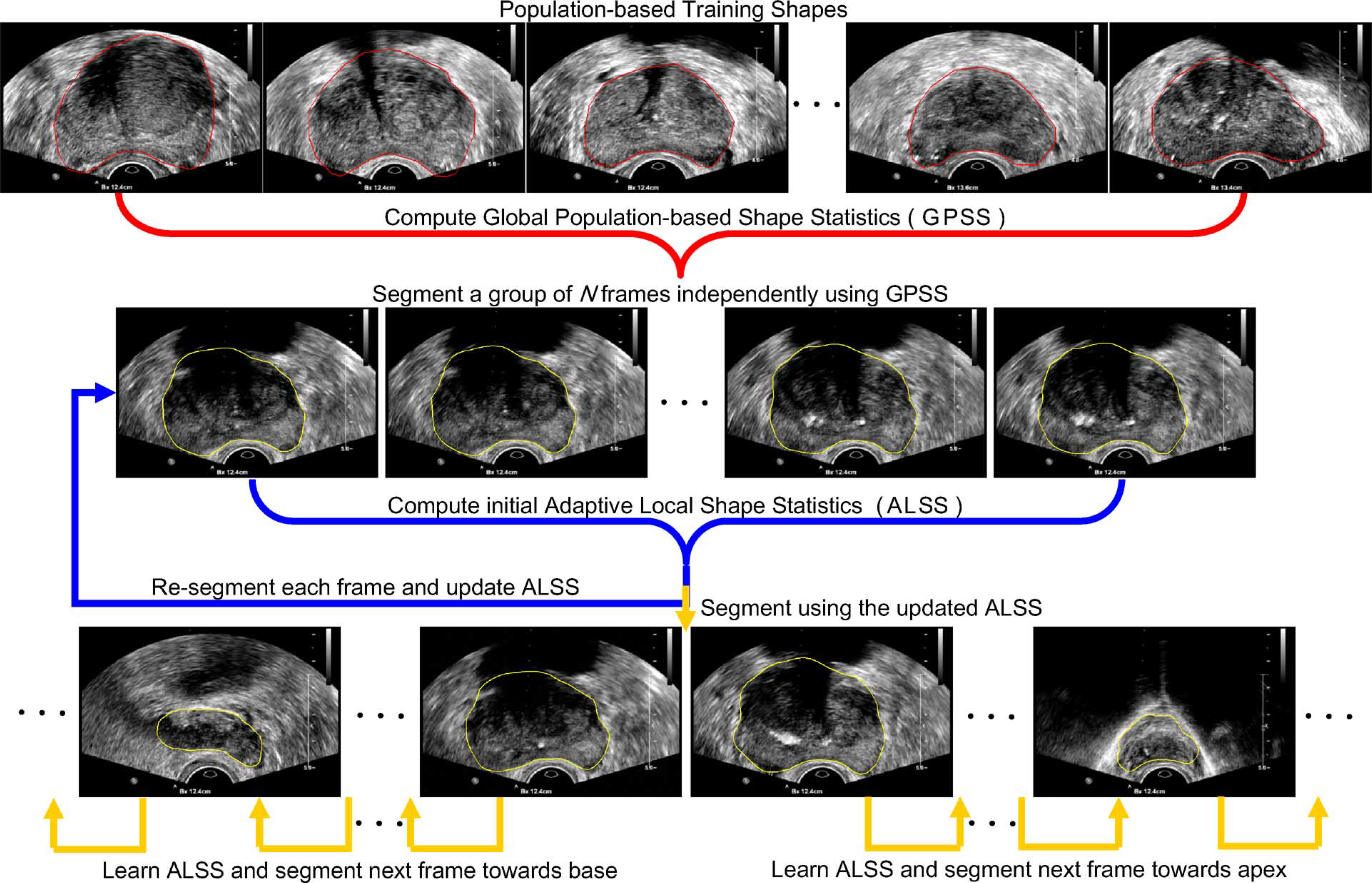
Overall scheme of the proposed TRUS video segmentation method.

As shown in the second row of Fig. 4, the deformable contour using ALSS will go back to segment the first frame of the video sequence, which is now considered as the (N + 1)th frame, with the previous segmentation result as the initialization. After the segmentation is done, the obtained prostate shape S_N will be added into the training shape set and shape S₀ will be removed. ALSS is learned by using the new set of training shapes and denoted as ${\mathbf{S}}_A^N$. With the updated ALSS, the deformable contour moves to segment the next frame with shape S_N as initialization. The learning and segmentation process is repeated until the whole video sequence is segmented.

IV. Experiments

A. Materials

The TRUS video sequences used in our experiments were obtained using an iU22 ultrasound system (Philips Healthcare, Andover, MA). The 2-D TRUS scan was performed from the base to the apex of the prostate in the axial orientation with a Philips C9-ultrasound probe. The TRUS images were digitized by using a video card. Each frame has 640 × 480 pixels. The pixel sizes of the frame-grabbed images were 0.15 and 0.18 mm in 4 and 5 cm depth settings, respectively. In our experiments, 19 video sequences with 3064 frames in total were grabbed from 19 different patients for prostate cancer biopsy. Manual segmentation performed by an experienced radiologist was considered as the ground truth for validation. Since the frames were continuously grabbed with a frame rate of 30 frames/s, the change between neighboring frames was small. Thus, the radiologist only manually segmented 301 frames from all the video sequences with equal temporal distance.

B. Parameter Setting

In our experiments, the deformable contour had n = 64 contour points. Three iterations of deformable segmentation were performed for each frame. The size of search range in each iteration was m = 11, i.e., five search points on each side of the contour. When doing deformable segmentation, all the energy terms in (8) were normalized into the range of [0, 1]. The weighting parameters in (10) and (11) were set to α = 0.4, β = 0.4, and γ = 0.5.

As a special parameter to our proposed method, the best training set size N for learning ALSS was determined by using an experiment. For each value of N between 1 and 20, ten randomly selected video sequences were segmented and quantitatively evaluated. Note that ALSS is the segmentation result of the previous frame when N = 1. The variation of performance by changing the value of N is shown in Fig. 5. The overall smoothed red curve clearly indicates that the segmentation error first decreased as N increased and then became larger and larger as N continued to increase after 6. The reason is that if too few shapes are used for learning ALSS, the segmentation may be too restrictive to the previous shapes and errors can be easily accumulated during the segmentation process. On the other hand, if the training shape set is too big, ALSS will not be able to quickly adapt to the shape changes and thus results in larger segmentation errors. Therefore, N = 6 was chosen in our experiments and ALSS-6 is used to indicate the proposed method for convenience.

Fig. 5.

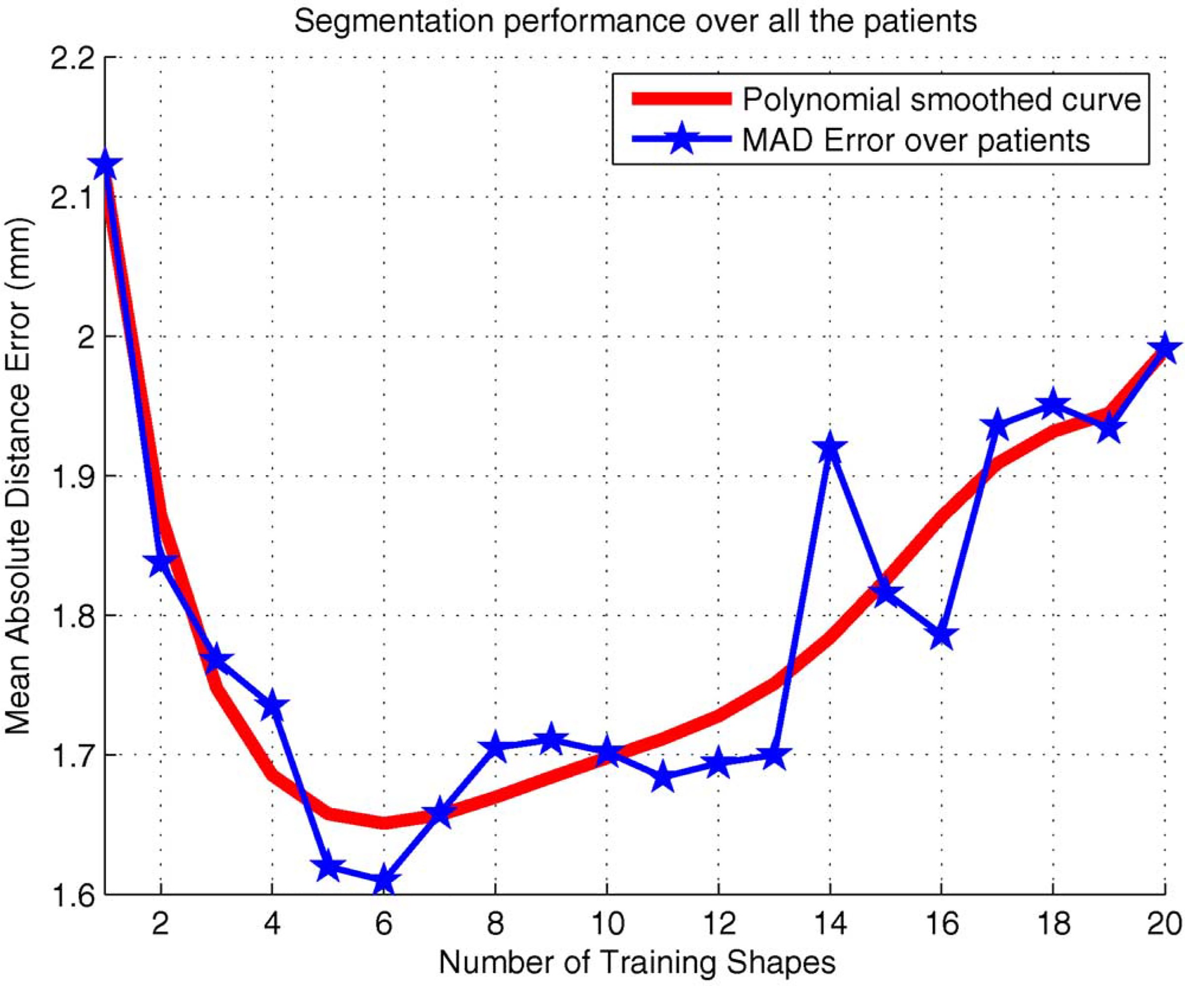
Variation of segmentation performance by changing the number of training shapes N for learning ALSS.

The proposed method was developed in C++ based on ITK [27]. The method segments TRUS video in a fully automatic fashion. In our experiments, it took about 200 ms for segmenting each frame on a Core2 1.86 GHz PC.

C. Evaluation Methods

For performance comparison, we also implemented two other methods with the same parameter settings as the proposed method. The first method was to independently segment all the frames using GPSS (the segmentation strategy in [10] and [11]), which is hereafter denoted as Method-1. The mean shape ${\overline{S}}_G$ in the GPSS was used to initialize the segmentation automatically. The second method had a very similar segmentation scheme as the proposed method but using only GPSS, which is denoted as Method-2 in the rest of the paper. Method-2 used the typical video segmentation strategy of propagating segmentation result of one frame to the next for initialization to take advantages of the similarity between the neighboring frames. The mean shape ${\overline{S}}_G$ in the GPSS was used to automatically initialize the segmentation in the first frame.

For quantitatively evaluating the performance of the segmentation methods, two measurement methods were used. One is the mean absolute distance (MAD) error. Let v_i and ${\mathbf{v}}_i^{\prime }$ denote the ith contour point from a segmented contour and the ground truth, respectively, after equally spaced distance-based sampling [24]. The MAD is defined as

$$\mathrm{MAD}=\frac{1}{n}\sum _{i=1}^n\Vert {\mathbf{v}}_i-{\mathbf{v}}_i^{\prime }\Vert .$$ (13)

Another quantitative measurement was the dice similarity coefficient (DSC) defined as

$$\mathrm{DSC}=\frac{2\left|A_s\cap A_g\right|}{\left|A_s\right|+\left|A_g\right|}$$ (14)

where A_s and A_g are the areas enclosed by the segmented contour and the ground truth, respectively. The standard deviation of the measurement was also computed to evaluate the variation of the segmentation results for each patient.

D. Experimental Results

All the 19 video sequences were segmented using the three methods, respectively. The results are shown in Table I. It can be seen that ALSS-6 outperformed the other two methods in all of the cases. In terms of the average MAD over all the 19 patients, the segmentation error of ALSS-6 was 51.8% smaller than that of Method-1 and was 21.9% smaller than that of Method-2. The improvement in both comparisons was significant. In our study, the statistical significance was evaluated using paired t test (p < 0.05). The DSC measurement was consistent with the MAD result in general.

TABLE I.

MAD (mm) and DSC Between the Ground Truth and Segmentations Done by the Three Different Methods Described in the Text on Each TRUS Video Sequence

Methods		Seq-1	Seq-2	Seq-3	Seq-4	Seq-5	Seq-6	Seq-7	Seq-8	Seq-9	Seq-10
Method-1	MAD	3.28	2.54	2.24	1.66	3.09	2.54	1.73	2.67	2.34	2.80
	DSC	0.79	0.84	0.87	0.88	0.81	0.85	0.87	0.83	0.86	0.82
Method-2	MAD	1.85	2.68	2.00	2.56	2.44	1.05	0.84	1.53	1.93	1.79
	DSC	0.90	0.84	0.89	0.86	0.84	0.89	0.92	0.87	0.87	0.86
ALSS-6	MAD	1.68	2.06	1.76	1.48	1.99	0.78	0.74	1.29	1.84	1.56
	DSC	0.92	0.88	0.92	0.90	0.87	0.92	0.94	0.89	0.91	0.90
Methods		Seq-11	Seq-12	Seq-13	Seq-14	Seq-15	Seq-16	Seq-17	Seq-18	Seq-19		Average
Method-1	MAD	1.66	1.20	3.01	1.63	3.02	4.73	1.92	2.97	2.53		2.53±0.81
	DSC	0.93	0.92	0.87	0.89	0.83	0.69	0.88	0.86	0.83		0.85±0.05
Method-2	MAD	2.30	1.19	2.71	1.68	2.90	1.99	2.13	3.09	1.54		2.01±0.63
	DSC	0.91	0.92	0.87	0.89	0.81	0.85	0.86	0.87	0.89		0.87±0.03
ALSS-6	MAD	1.69	1.02	2.17	1.76	2.66	1.82	1.65	1.92	1.47		1.65 ±0.47
	DSC	0.95	0.93	0.91	0.93	0.84	0.88	0.90	0.92	0.90		0.91±0.03

To show the robustness of the proposed method to initialization, we performed a set of experiments by varying the mean shape with random translation along X and Y axes (up to 10 pixels), scaling (up to 15%), and rotation (up to 15°), respectively, as shown in Fig. 6. The segmentation results had no significant change (p > 0.05) in ten runs.

Fig. 6.

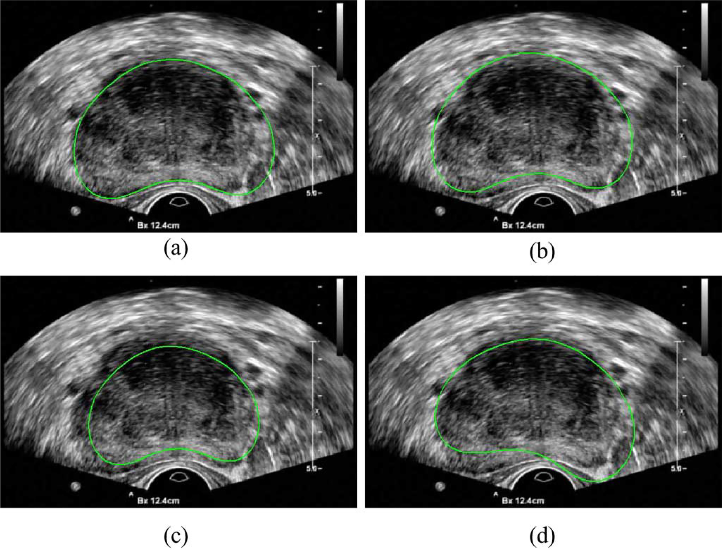
Automatic initialization of the segmentation by (a) using the mean shape ${\overline{S}}_G$ of the GPSS, (b) with translation, (c) with scaling, and (d) with rotation.

We also compared the performance of the three methods in the base, midgland, and apex regions separately. Fig. 7 shows some segmentation results of a TRUS video sequence in different regions. It can be seen that the segmentation results of ALSS-6 are generally very close to the prostate boundaries, while the other two methods are not very accurate, especially in the base and apex areas. For quantitative evaluation, the ground truth segmentations of each patient were sequentially divided into three groups with equal number of frames in each group. Since the video sequence was obtained by scanning through the prostate from the base to apex, the three groups were labeled as base, midgland, and apex in the specified order. The evaluation results are shown in Table II. Compared to Method-1 and Method-2, the segmentation performance was significantly improved in all the regions by using ALSS-6.

Fig. 7.

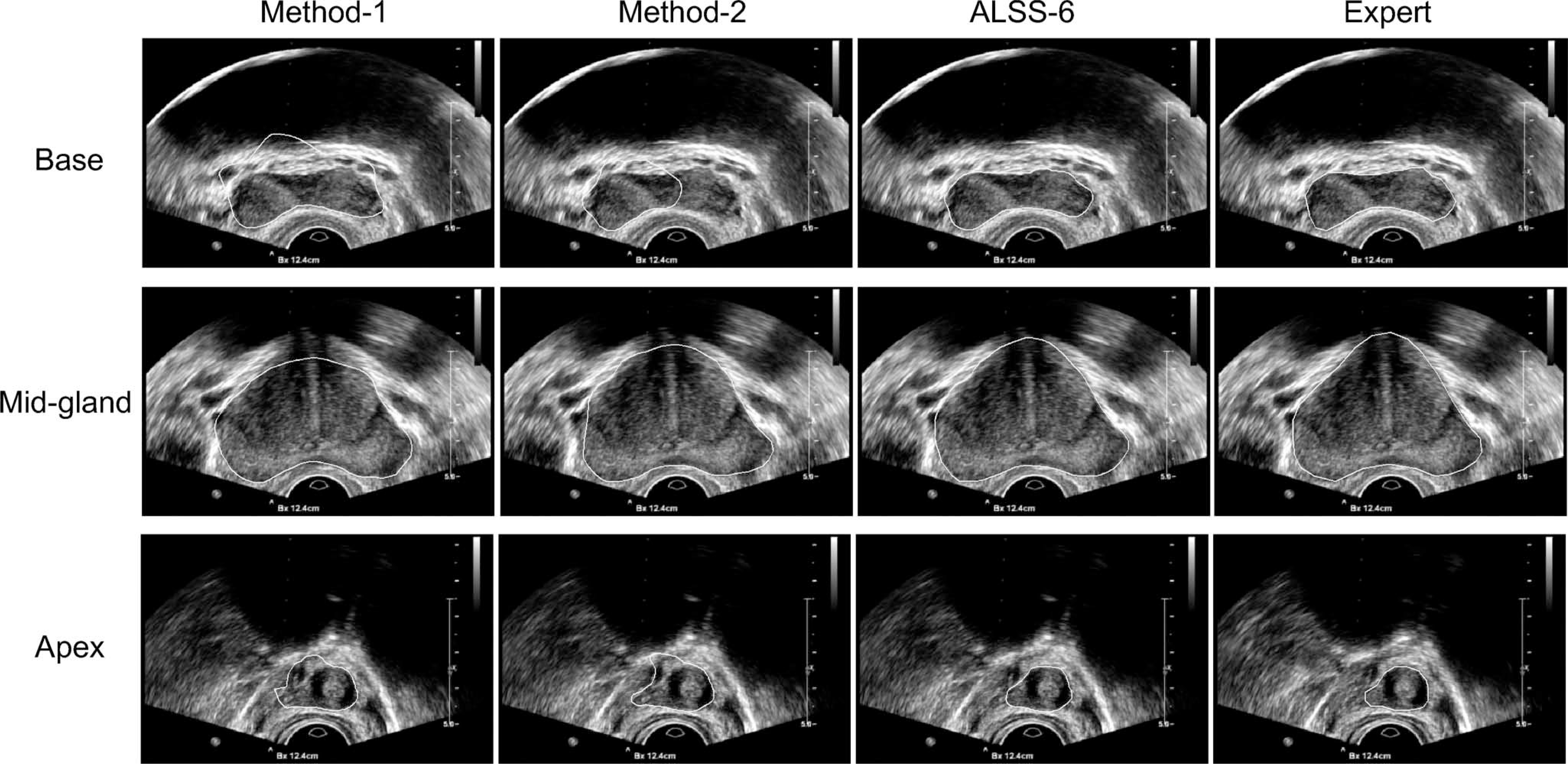
Some segmentation results from the base, midgland, and apex regions obtained by using the three different methods (see the text) and by the expert, respectively.

TABLE II.

MAD Errors (mm) of the Three Different Methods (Described in the Text) in the Base, Midgland, and Apex Areas Over the 19 Video Sequences, Respectively

Region	Method-1	Method-2	ALSS-6
base	2.44±1.16	1.94±1.04	1.63±0.74
mid-gland	1.46±0.57	1.45±0.54	1.21±0.49
apex	3.55±1.66	2.68±1.00	2.28±0.84

The performance improvement of ALSS-6 in the base and apex regions is obvious. Compared to Method-1 and Method-2, ALSS-6 reduced the MAD errors by 49.4% and 18.9% in the base and by 55.6% and 17.7% in the apex, respectively. It can also be observed that Method-2 performed better than Method-1 in the base and apex regions using the same GPSS. The reason is that Method-2 adaptively exploited the similarity between neighboring frames by using the segmented shape from the previous frame to initialize the segmentation of the next frame, while Method-1 treated each frame independently. By initializing the segmentation in the same way as Method-2, ALSS-6 obtained smaller segmentation errors because the large shape variations of the prostate in those areas were effectively captured by ALSS.

The performance of the three methods in the midgland region is also interesting. The results obtained by using Method-1 and Method-2 have no significant difference, which suggests that the similarity between neighboring frames was not very useful when segmenting the midgland. Compared to those two methods, however, ALSS-6 performed significantly better by reducing the segmentation errors by 20.8% and 19.4%, respectively. This is due to the fact that ALSS is patient specific and thus leads to better segmentation results than GPSS.

E. Discussion

The advantages of the proposed method are threefold. First, ALSS can provide more accurate prostate shape constraint for segmenting a TRUS video sequence, because it is learned from the patient’s own data and thus specific to the subject. More importantly, compared to the work in [21] where all the segmented shapes were used to compute patient-specific global shape statistics, ALSS is more sensitive to the local shape changes as the TRUS probe moves to scan different regions of the prostate, since only shapes from the previous N frames are used for learning. This can significantly improve the prostate segmentation performance in the base and apex areas, by overcoming the large and rapid shape variations of the prostate in those areas. Finally, the proposed method is robust to the initialization. In general, a deformable contour using GPSS can obtain good segmentation results in the midgland area [10], [11]. In our study, we use the mean shape ${\overline{S}}_G$ from the GPSS to automatically initialize the segmentation. After the initial N frames are independently segmented with GPSS, ALSS is obtained and used to resegment those frames, which can further prevent the segmentation from being led by an accidentally bad initialization.

V. Conclusion

In this paper, we proposed learning local shape statistics adaptively for segmenting the prostate in 2-D TRUS video sequences. By incorporating ALSS into a deformable contour, more accurate segmentation results were obtained for whole prostate segmentation as compared to other previous techniques. In particular, segmentation performance in the base and apex regions was significantly improved. To the best of our knowledge, this is the first method in the field that can successfully segment the base and apex of the prostate in 2-D TRUS by using the patient-specific and locally adaptive shape statistics. Application of the proposed segmentation strategy to 3-D ultrasound video segmentation may be investigated in our future work.

References

- [1].American Cancer Society. (2010). “What are the key statistics about prostate cancer?” [Online]. Available: http://www.cancer.org/.
- [2].Shen D, Lao Z, Zeng J, Zhang W, Sesterhenn IA, Sun L, Moul JW, Herskovits EH, Fichtinger G, and Davatzikos C, “Optimized prostate biopsy via a statistical atlas of cancer spatial distribution,” Med. Image Anal, vol. 8, pp. 139–150, 2003. [DOI] [PubMed] [Google Scholar]
- [3].Kadoury S, Yan P, Xu S, Glossop ND, Choyke PL, Turkbey B, Pinto P, Wood BJ, Kruecker J, “Realtime TRUS/MRI fusion targeted-biopsy for prostate cancer: A clinical demonstration of increased positive biopsy rates,” in Prostate Cancer Imaging (ser. Lecture Notes in Computer Science), vol. 6367, New York: Springer-Verlag, 2010, pp. 52–62. [Google Scholar]
- [4].Yan P, Xu S, Turkbey B, and Kruecker J, “Discrete deformable model guided by partial active shape model for TRUS image segmentation,” IEEE Trans. Biomed. Eng, vol. 57, no. 5, pp. 1158–1166, May 2010. [DOI] [PMC free article] [PubMed] [Google Scholar]
- [5].Shao F, Ling KV, Ng WS, and Wu R, “Prostate boundary detection from ultrasonographic images,” J. Ultrasound Med, vol. 22, pp. 605–623, 2003. [DOI] [PubMed] [Google Scholar]
- [6].Nobel JA and Boukerroui D, “Ultrasound image segmentation: A survey,” IEEE Trans. Med. Imag, vol. 25, no. 8, pp. 987–1010, August. 2006. [DOI] [PubMed] [Google Scholar]
- [7].Abolmaesumi P and Sirouspour MR, “An interacting multiple model probabilistic data association filter for cavity boundary extraction from ultrasound images,” IEEE Trans. Med. Imaging, vol. 23, no. 6, pp. 772–784, June. 2004. [DOI] [PubMed] [Google Scholar]
- [8].Gong L, Pathak SD, Haynor DR, Cho PS, and Kim Y, “Parametric shape modeling using deformable superellipses for prostate segmentation,” IEEE Trans. Med. Imag, vol. 23, no. 3, pp. 340–349, March. 2004. [DOI] [PubMed] [Google Scholar]
- [9].Badiei S, Salcudean SE, Varah J, and Morris WJ, “Prostate segmentation in 2D ultrasound images using image warping and ellipse fitting,” in Proc. Mid. Image Comput. Comput.-Assisted Intervention Conf. (MICCAI), 2006, vol. 4191, pp. 17–24. [DOI] [PubMed] [Google Scholar]
- [10].Ladak HM, Mao F, Wang Y, Downey DB, Steinman DA, and Fenster A,“Prostateboundarysegmentationfrom2Dultrasoundimages,” Med. Phys, vol. 27, no. 8, pp. 1777–1788, 2000. [DOI] [PubMed] [Google Scholar]
- [11].Shen D, Zhan Y, and Davatzikos C, “Segmentation of prostate boundaries from ultrasound images using statistical shape model,” IEEE Trans. Med. Imaging, vol. 22, no. 4, pp. 539–551, April. 2003. [DOI] [PubMed] [Google Scholar]
- [12].Cosío FA, “Automatic initialization of an active shape model of the prostate,” Med. Image Anal, vol. 12, no. 4, pp. 469–483, 2008. [DOI] [PubMed] [Google Scholar]
- [13].Wang Y, Cardinal HN, Downey DB, and Fenster A, “Semiautomatic three-dimensional segmentation of the prostate using two-dimensional ultrasound images,” Med. Phys, vol. 30, pp. 887–897, May 2003. [DOI] [PubMed] [Google Scholar]
- [14].Zhan Y and Shen D, “Deformable segmentation of 3-D ultrasound prostate images using statistical texture matching method,” IEEE Trans. Med. Imag, vol. 25, no. 3, pp. 256–272, March. 2006. [DOI] [PubMed] [Google Scholar]
- [15].Ray N and Acton S, “Data acceptance for automated leukocyte tracking through segmentation of spatiotemporal images,” IEEE Trans. Biomed. Eng, vol. 52, no. 10, pp. 1702–1712, October. 2005. [DOI] [PubMed] [Google Scholar]
- [16].Yan P, Xu S, Turkbey B, and Kruecker J, “Segmenting TRUS video sequences using local shape statistics,” in Medical Imaging 2010: Visualization, Image-Guided Procedures and Modeling. vol. 7625, Bellingham, WA: SPIE, 2010, p. 762514. [Google Scholar]
- [17].Yan P and Kruecker J, “Incremental shape statistics learning for prostate tracking in TRUS,” in Proc. Int. Conf. Med. Image Comput. Comput.-Assisted Intervention (MICCAI), 2010, vol. 13, no. 2, pp. 42–49. [DOI] [PubMed] [Google Scholar]
- [18].Jacob G, Noble JA, Behrenbruch CP, Kelion AD, and Banning AP, “A shape-space based approach to tracking myocardial borders and quantifying regional left ventricular function applied in echocardiography,” IEEE Trans. Med. Imag, vol. 21, no. 3, pp. 226–238, March. 2002. [DOI] [PubMed] [Google Scholar]
- [19].Sun W, Çetin M, Chan R, Reddy V, Holmvang G, Chandar V, and Willsky AS, “Segmenting and tracking the left ventricle by learning the dynamics in cardiac images,” in Proc. Inf. Process. Med. Imag. Conf. (IPMI), 2005, pp. 553–565. [DOI] [PubMed] [Google Scholar]
- [20].Zhu Y, Papademetris X, Sinusas AJ, and Duncan JS, “A dynamical shape prior for LV segmentation from RT3D echocardiography,” in Proc. Int. Conf. Med. Image Comput. Comput.-Assisted Intervention (MICCAI), 2009, vol. 12, no. 1, pp. 206–213. [DOI] [PMC free article] [PubMed] [Google Scholar]
- [21].Shi Y, Qi F, Xue Z, Chen L, Ito K, Matsuo H, and Shen D, “Segmenting lung fields in serial chest radiographs using both population-based and patient-specific shape statistics,” IEEE Trans. Med. Imag, vol. 27, no. 4, pp. 481–494, April. 2008. [DOI] [PubMed] [Google Scholar]
- [22].Feng Q, Foskey M, Chen W, and Shen D, “Segmenting CT prostate images using population and patient-specific statistics for radiotherapy,” Med. Phys, vol. 37, no. 8, pp. 4121–4132, 2010. [DOI] [PMC free article] [PubMed] [Google Scholar]
- [23].Cootes TF, Taylor CJ, Cooper DH, and Graham J, “Active shape models: Their training and application,” Comput. Vis. Image Understand, vol. 61, no. 1, pp. 38–59, January. 1995. [Google Scholar]
- [24].Hodge AC, Fenster A, Downey DB, and Ladak HM, “Prostate boundary segmentation from ultrasound images using 2-D active shape models: Optimisation and extension to 3-D,” Comput. Methods Programs Biomed, vol. 84, pp. 99–113, 2006. [DOI] [PubMed] [Google Scholar]
- [25].Williams DJ and Shah M, “A fast algorithm for active contours and curvature estimation,” CVGIP: Image Understand, vol. 55, no. 1, pp. 14–26, 1992. [Google Scholar]
- [26].Amini AA, Weymouth TE, and Jain RC, “Using dynamic programming for solving variational problems in vision,” IEEE Trans. Pattern Anal. Mach. Intell, vol. 12, no. 9, pp. 855–866, September. 1990. [Google Scholar]
- [27].Ibanez L, Schroeder W, Ng L, and Cates J. (2005). The ITK Software Guide, 2nd ed. Kitware, Inc., [Online]. Available: http://www.itk.org/ItkSoftwareGuide.pdfs [Google Scholar]