Discrete Deformable Model Guided by Partial Active Shape Model for TRUS Image Segmentation

Abstract

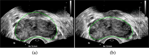
Automatic prostate segmentation in transrectal ultrasound (TRUS) images is highly desired in many clinical applications. However, robust and automated prostate segmentation is challenging due to the low SNR in TRUS and the missing boundaries in shadow areas caused by calcifications or hyperdense prostate tissues. This paper presents a novel method of utilizing a priori shapes estimated from partial contours for segmenting the prostate. The proposed method is able to automatically extract prostate boundary from 2-D TRUS images without user interaction for shape correction in shadow areas. During the segmentation process, missing boundaries in shadow areas are estimated by using a partial active shape model, which takes partial contours as input but returns a complete shape estimation. With this shape guidance, an optimal search is performed by a discrete deformable model to minimize an energy functional for image segmentation, which is achieved efficiently by using dynamic programming. The segmentation of an image is executed in a multiresolution fashion from coarse to fine for robustness and computational efficiency. Promising segmentation results were demonstrated on 301 TRUS images grabbed from 19 patients with the average mean absolute distance error of 2.01 mm ± 1.02 mm.

I. INTRODUCTION

Prostate cancer is the second most common cancer among American men after skin cancer. It is the second leading cause of cancer death in men in the United States [1]. Transrectal ultrasound (TRUS) is the most frequently used method for image-guided biopsy and therapy of prostate cancer due to its real-time nature, low cost, and simplicity [2]. Accurate segmentation of the prostate can play a key role in many procedures, such as biopsy needle placement [3], biopsy and therapy planning [4], and motion monitoring [5], [6]. However, segmentation of prostate boundaries from TRUS images is a difficult task.

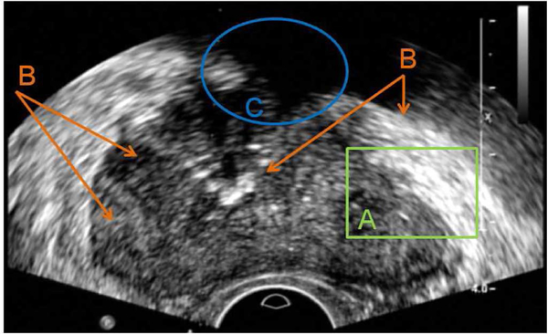
For a prostate segmentation method to succeed, the following challenges of TRUS shown in Fig. 1 have to be properly addressed. First of all, compared to computed tomography (CT) or magnetic resonance (MR) images, the SNR of TRUS images is much lower, which often causes algorithms relying on single pixels to fail. Second, pixel intensity distributions are inhomogeneous both inside and outside of the prostate. Regions with similar contrast and intensity distributions can be observed in both prostate and nonprostate areas. The same type of tissue may have quite different pixel intensities and contrast at different parts. Therefore, there is no global characterization of prostate and nonprostate areas, which makes it hard to directly differentiate the prostate from surrounding tissues based on pixel intensities and region appearances. Finally, shadow artifacts often appearing at the anterior side of the prostate make the segmentation difficult because of the lack of image information in those areas [7].

Fig. 1.

Major challenges for segmentation of prostate boundaries from TRUS images. (a) Low SNR. (b) Large intensity variation inside of the prostate, and similarity between prostate and nonprostate tissues. (c) Shadow artifact where no boundary is available.

A number of prostate segmentation methods were reported in the past decade, which usually require expert interaction during the process by either initializing contours or adjusting segmentation results for successful segmentation [8], [9]. Among the reported methods, deformable-model- and statistical-shape-model-based algorithms demonstrated the most promising segmentation results. Badiei et al. [10] presented a semiautomatic segmentation method by warping ellipses to fit the detected edges in TRUS images. The method took advantage of the similarity between the prostate’s shape and the warped ellipse. Although the method is simple and efficient, its application is limited to images in midgland region with regular shapes. In addition, it needs six points selected from specific locations to initialize the algorithm. A 2-D semiautomatic discrete dynamic contour (DDC) model for prostate boundary segmentation was presented by Ladak et al. [11]. The DDC deforms in the prostate image to extract boundary starting from an initial contour defined by four manually picked points. Wang et al. [12] extended the method to 3-D segmentation, but it requires manually editing the segmentation results to get required accuracy. Shen et al. [13] and Zhan and Shen [14] presented automatic segmentation methods for extracting prostate contour/surface from 2-D and 3-D US images. Spatially adaptive Gabor support vector machine (G-SVM) was developed to classify texture patterns extracted by rotation invariant Gabor filter bank. Statistical shape model was then fit to the output image of G-SVM to get prostate boundary in the image. However, due to the use of G-SVM, the method is computationally intensive and may not be appropriate for TRUS-guided prostate interventions. In addition, as other automatic segmentation algorithms [15], [16], the algorithm demonstrated only on images without significant shadow artifacts.

In this paper, we propose a new automatic segmentation method for extracting prostate boundaries from 2-D TRUS images by using a partial active shape model (PASM) with a discrete deformable model (DDM) to address the aforementioned challenges. For computational efficiency, a coarse-to-fine multiresolution strategy is used in both initialization and contour deformation. When segmenting an image, as opposed to approximating a whole prostate boundary in the traditional shape-estimation methods proposed in [12], [17], and [13], PASM only uses some parts of the prostate contour with salient boundary features for shape estimation to avoid the misleading information produced by shadows. After this, DDM searches for the global minimum in a defined range under the guidance of shape prior, which is estimated by using PASM. The proposed method is able to extract a complete prostate boundary even when part of the boundary is missing due to imaging shadows, which was previously manually corrected by user interaction as in other works [12], [17].

The rest of this paper is organized as follows. The selected prostate boundary feature is presented in Section II. The proposed algorithms of PASM and DDM are presented in Sections III and IV, respectively. Section V summarizes the integrated multiresolution segmentation method. The segmentation performance of the proposed method is demonstrated in Section VI with quantitative evaluation on TRUS images. We conclude the work in Section VII.

II. PROSTATE BOUNDARY FEATURE EXTRACTION

The proposed segmentation method consists of two major components, the prostate shape fitting using PASM and the deformable segmentation using DDM. Since prostate boundary feature plays a key role in both components, feature extraction is first presented.

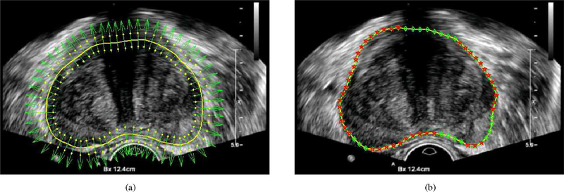
In TRUS images, the most noticeable feature of the prostate boundary is the dark-to-bright transition from the inside to the outside of the prostate. In order to extract this feature, the normal vector profile (NVP) is used [17]. In our work, each contour is represented by a set of sequential points. Let $\overrightarrow{n}=\left(n_x,n_y\right)$ denote the normal direction of a contour at point (x, y), which is pointing from inside to outside, as shown in Fig. 2(a). NVP is a vector f = [f₁, f₂, …, f_2m]^T. Element f_i is the intensity of the ith pixel at location (x_i, y_i) = (x + (i − m)n_x, y + (i − m)n_y ).

Fig. 2.

(a) Normal vector and two candidate points in the normal vector profile of each contour point are shown in the figure for illustration. (b) Contour is composed by a series of contour points as shown in green diamond and the detected salient contour points are shown in red pentagon.

Algorithm 1.

Partial Salient Contour Detection

- Get all the salient contour points whose NVP contrast c is smaller than −1.

- Estimate the intensity distribution of the prostate according to the shape initialization.

- Compute the mean value of NVPs. If the value is smaller than the lower boundary of the prostate’s intensity range, remove the point from the salient point set, since this is likely to be in shadow area.

- Apply ID median filter to the point list and remove isolated points, which are often caused by noise.

To detect the dark-to-bright transition, the contrast of NVP f is computed as c = p^T · f/2m, where p is a vector defined as [1, …, 1, −1, …,−1]^T with length 2m. The saliency of each contour point is measured by the contrast c of NVP. A contour point is considered to be salient if c is smaller than a threshold. In our work, the threshold is selected as −1, which ensures the minimum amount of the dark-to-bright transition and is able to exclude some noise points. Contour parts containing the consecutive salient contour points are then detected by using Algorithm 1. A detection example is shown in Fig. 2(b).

III. PARTIAL ACTIVE SHAPE MODEL

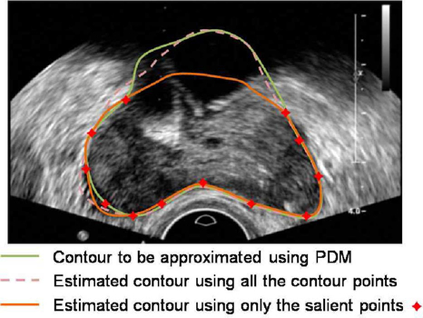
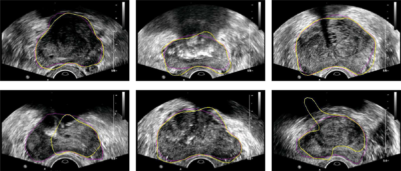
Shape priors can be very useful in guiding image segmentation, especially when the boundaries to be segmented are not clear because of the low SNR, limited image resolution, or missing boundary information [18]. During the segmentation process, the shape prior of an object can be estimated by using the shape statistics according to an input contour. However, due to the commonly observed shadow artifacts in TRUS images, an incorrect shape may be estimated based on an input contour, which is far away from the desired segmentation result, as shown in Fig. 3. It will be hard to obtain a reasonable segmentation in the following steps with this misleading shape estimation. Some segmentation results due to bad shape estimation are shown in Fig. 4. In order to solve the problem, a new PASM is proposed in this paper. The idea is to use only those salient contour points for shape estimation, which may provide better estimation than using the whole contour. In the following sections, we present the details of computing shape statistics using the point distribution model (PDM) and estimating the shape prior using PASM.

Fig. 3.

Illustration of prostate shape estimation from salient partial contour. Due to the shadow artifacts, which are commonly observed in TRUS images, the given initial contour may be far from the desired contour. A misleading shape can be estimated by using the whole initial contour. While using only the salient partial contours, a more reasonable shape estimation can be obtained.

Fig. 4.

Example segmentation results of the prostate from ultrasound images without PASM. Shape priors are estimated by using the whole contour during the segmentation process. Yellow contours show the automatic segmentation results and the ground truth is shown in magenta.

A. Computing Prostate Shape Statistics

PDM has been successful in modeling shape statistics since it was introduced by Cootes et al. [19]. PDM is a statistical approach able to extract a compact representation from a set of training instances. In PDM, each planar shape is represented by n 2-D points as the vector

$$\mathbf{X}={\left[x_1,x_2,\dots ,x_n;y_1,y_2,\dots ,y_n\right]}^T.$$ (1)

Thus, each shape is an observation in the 2n dimensional space. Fig. 5 shows a set of training images with prostate contour manually outlined. In our work, the contour points are equally spaced (Euclidean-distance-based spacing) sampled from the shapes.

Fig. 5.

Build the PDM from contour points on a set of manual segmentation results. Each planar shape x_i is represented by n points along the contour.

After normalization [13], principal component analysis (PCA) is used to account for the redundancy in the m input data after alignment. The resulting shape model consists of a function of the mean shape $\overline{\mathbf{X}}$ and a matrix Φ, which includes the most significant t eigenvectors of the covariance matrix of the input data as, shown in (2) at the bottom of the page.

$$\mathrm{\Phi }={\left[\begin{array}{cccccccccc}{e}_{11}& e_{12}& e_{13}& e_{14}& e_{15}& e_{16}& \dots & \dots & e_{12n-1}& e_{12n}\\ e_{21}& e_{22}& e_{23}& e_{24}& e_{25}& e_{26}& \dots & \dots & e_{22n-1}& e_{22n}\\ & & ⋮& & & ⋮& \dots & \dots & & ⋮\\ e_{t1}& e_{t2}& e_{t3}& e_{t4}& e_{t5}& e_{t6}& \dots & \dots & e_{t2n-1}& e_{t2n}\end{array}\right]}^T$$ (2)

The modes are ordered according to the percentage of variation that they explain. In our work, we set the percentage threshold as 98% of the total variation to choose the number of modes. With PDM, a new shape x can be decomposed by using the mean shape and the eigenvectors to be compactly represented by a parameter vector b as

$$\mathbf{b}={\mathbf{\Phi }}^T(\mathbf{x}-\overline{\mathbf{x}}).$$ (3)

The approximation of the shape in the training shape space is obtained by linearly combining the eigenvectors as

$$\widehat{\mathbf{x}}=\overline{\mathbf{x}}+\mathrm{\Phi }\mathbf{b}$$ (4)

which can be used to estimate shape prior in the segmentation process.

B. Estimating Shape Prior From Salient Partial Contour

If the whole contour is used for shape estimation, an estimated shape can be obtained by using (3) and (4). However, in order to deal with the shadow artifacts, only the partial salient contour will be used for shape estimation. Therefore, a new method is proposed in our paper.

Let x_s denote the salient contour parts of a contour x detected by the method in Section II. ${\overline{\mathbf{x}}}_s$ and Φ_s are the corresponding points of those salient parts in the mean shape $\overline{\mathbf{X}}$ and the eigenvectors matrix Φ, respectively, after removing the nonsalient parts, i.e.,

$${\overline{\mathbf{x}}}_s={\left[{\overline{x}}_1,{\overline{x}}_2,{\overline{\cancel{x}}}_3,{\overline{\cancel{x}}}_4,\dots ,{\overline{x}}_n;{\overline{y}}_1,{\overline{y}}_2,{\overline{y}}_3,{\overline{y}}_4,\dots ,{\overline{y}}_n\right]}^T$$ (5)

$${\mathrm{\Phi }}_s={\left[\begin{array}{cccccccccc}{e}_{11}& e_{12}& {\cancel{e}}_{13}& {\cancel{e}}_{14}& {\cancel{e}}_{15}& e_{16}& \dots & \cancel{·}··& {\cancel{e}}_{12n-1}& e_{12n}\\ e_{21}& e_{22}& {\cancel{e}}_{23}& {\cancel{e}}_{24}& {\cancel{e}}_{25}& e_{26}& \dots & \cancel{·}··& {\cancel{e}}_{22n-1}& e_{22n}\\ & & \cancel{⋮}& & \cancel{⋮}& & \dots & \cancel{·}··& & ⋮\\ e_{t1}& e_{t2}& {\cancel{e}}_{t3}& {\cancel{e}}_{t4}& {\cancel{e}}_{t5}& e_{t6}& \dots & \cancel{·}··& {\cancel{e}}_{t2n-1}& e_{t2n}\end{array}\right]}^T$$ (6)

and as shown in (6), at the bottom of the next page.

According to (4), the partial contour can be represented by

$${\mathbf{x}}_s={\overline{\mathbf{x}}}_s+{\mathbf{\Phi }}_s{\mathbf{b}}_s+ϵ$$ (7)

where ϵ is the approximation error. The parameter vector b_s can be computed by minimizing the mean square of the error E = ǁϵǁ², which yields

$$\arg \underset{{\mathbf{b}}_s}{\min }E=\arg \underset{{\mathbf{b}}_s}{\min }{\Vert {\mathbf{x}}_s-{\overline{\mathbf{x}}}_s-{\mathbf{\Phi }}_s{\mathbf{b}}_s\Vert }^2.$$ (8)

Differentiating both sides of (8) with respect to b_s results in

$$\frac{\partial E}{\partial {\mathbf{b}}_s}=2{\mathbf{\Phi }}_s^T{\mathbf{\Phi }}_s{\mathbf{b}}_s-2{\mathbf{\Phi }}_s^T\left({\mathbf{x}}_s-{\overline{\mathbf{x}}}_s\right).$$ (9)

The mean square error E is minimized when the left side of (9) equals to 0. Therefore, the coefficients b_s can be computed by using Moore–Penrose inverse as

$${\mathbf{b}}_s={\left({\mathbf{\Phi }}_s^T{\mathbf{\Phi }}_s\right)}^{-1}{\mathbf{\Phi }}_s^T\left({\mathbf{x}}_s-{\overline{\mathbf{x}}}_s\right).$$ (10)

The estimated shape from PASM is generated by replacing the coefficients b in (4) with b_s

$$\widehat{\mathbf{x}}=\overline{\mathbf{x}}+\mathbf{\Phi }{\mathbf{b}}_s.$$ (11)

Unlike the previous work on partial PCA [20]– [23], where partial training data are used and the eigenvectors are computed using the EM method, our method uses complete training contours to build a PDM. In addition, the proposed method takes partial contour as input and gives a complete contour as output. The shape $\widehat{\mathbf{x}}$ estimated from (11) has two desired properties. First, the estimated shape is an approximation to the partial salient contour x_s by fitting the corresponding parts of the shape statistics to it by minimizing the mean square error E. Second, the estimated shape is an interpolation of the shape statistics with weights b_s for the components in the rest of the contour.

IV. DISCRETE DEFORMABLE MODEL

Under the guidance of shape prior estimated by using PASM, deformable model is employed to segment TRUS images for extracting boundaries. However, it is computationally inhibitive to compute the NVP features at every pixel location with all the possible orientations, which is required by the traditional deformable model [24]. Thus, a DDM is proposed. In order to deform the shape model efficiently for minimizing the energy function, an optimal search is performed by using dynamic programming, which greatly reduces the computational complexity and guarantees the global minimum inside the search range.

The proposed DDM consists of a shape model represented by a series of points, with an associated energy function. The prostate is segmented from TRUS images by deforming the DDM by moving the model points to minimize the energy. In our study, for each model point, the energy function consists of three terms: the external image feature term, the internal contour continuity and curvature term, and the PASM shape guidance term

$$E\left(v_i\right)=E_{\text{ext}}\left(v_i\right)+E_{\text{int}}\left(v_i\right)+E_{\text{PASM}}\left(v_i\right).$$ (12)

The external energy E_ext(v_i) is defined by the contrast of NVP features and attracts the contour toward the prostate boundary defined by dark-to-bright transition, as in Section II

$$E_{\text{ext}}\left(v_i\right)={\mathbf{p}}^T\cdot \mathbf{f}.$$ (13)

The internal energy E_int(v_i) is defined by the model continuity and curvature, and used to preserve the geometric shape of the model during deformation. In our paper, we consider the case when E_int(v_i) includes the second-order term, i.e., the computation of E_int(v_i) involves the model points v_i−1 and v_i+1. The internal energy term can be computed as

$$\begin{gathered} E_{\text{int}}\left(v_i\right)=\alpha \left(\Vert v_i-v_{i-1}\Vert +\Vert v_{i+1}-v_i\Vert -2d\right) \\ +\beta \Vert \left(v_i-v_{i-1}\right)-\left(v_{i+1}-v_i\right)\Vert \end{gathered}$$ (14)

where α and β are the weights of the continuity and curvature, respectively, and d is the average distance between neighboring model points. The first term at the right side of (14) tends to keep the contour points from either too close or too far. The second term smooths the model by penalizing sharp angles.

The PASM term is defined by the distance between point v_i from the model and the corresponding point $v_i^{\prime }$ on the estimated shape using PASM

$$E_{\text{PASM}}\left(v_i\right)=\gamma \Vert v_i-v_i^{\prime }\Vert$$ (15)

where γ is a positive weighting parameter. Besides guiding the deformable model to get smoother contour and to overcome imaging noise, the PASM term drives the deformable model toward the estimated shape prior in the shadow areas.

The total energy function that DDM seeks to minimize is the sum of the energy at each model point

$$\begin{gathered} E_{\text{total}}\left(v_1,v_2,\dots ,v_n\right)=E_1\left(v_n,v_1,v_2\right)+E_n\left(v_{n-1},v_n,v_1\right) \\ +\sum _{i=2}^{n-1}{E}_i\left(v_{i-1},v_i,v_{i+1}\right). \end{gathered}$$ (16)

To efficiently minimize the energy function (16), dynamic programming [25], [26] is employed by DDM to perform an optimal search for the global minimum in a defined range. Dynamic programming will give the same result as the global search, but with much lower computational complexity. Furthermore, unlike the traditional deformable model [24], dynamic programming is not moving the model points one by one, but searching over the whole specified space. It helps DDM to avoid being trapped by local minimum. Therefore, DDM is able to catch the prostate boundary even if the initialized contour is not close to the boundary.

V. MULTIRESOLUTION SEGMENTATION FRAMEWORK

In this section, we present the details of our automatic initialization algorithm and the overall integrated segmentation framework.

A. Initialization

Initialization is a very important step in automatic deformable segmentation. For an algorithm to successfully extract the prostate boundary, the initialized contour is required to be close to the boundary of interest. Initialization should also be fast and robust. The initialization process proposed in this paper is guided by the NVP features and the PDM to exploit both the dark-to-bright transition and shape statistics. Unlike most other model-based techniques, which require a manual initialization to start the model fitting, we use an automatic initialization method. To increase the capture range and the efficiency of the initialization process, a coarse-to-fine pyramid approach is used. In our method, the mean shape of the training models is first used as a seed contour. It is downsized to fit the coarsest level to start the initialization.

At each resolution level, the contour points of the seed model move along the normal direction to find the dark-to-bright transition. After all the points have moved, partial salient contour x_s can be detected, as described in Section II. By using x_s and the corresponding mean shape parts ${\overline{x}}_s$ in PDM, a similarity transformation T_s can be computed by

$$\left[\begin{array}{lll}{x}_1,\hfill & \dots ,\hfill & x_m\hfill \\ y_1,\hfill & \dots ,\hfill & y_m\hfill \end{array}\right]\approx {\mathbf{T}}_s\left[\begin{array}{lll}{\overline{x}}_1,\hfill & \dots ,\hfill & {\overline{x}}_m\hfill \\ {\overline{y}}_1,\hfill & \dots ,\hfill & {\overline{y}}_m\hfill \end{array}\right]$$ (17)

where m denotes the number of salient contour points. The transformed shape ${\mathbf{T}}_s\overline{\mathbf{x}}$ is then used as the initialization result at the current level. The shape obtained at the finest level is considered as the final initialization result. An example of initialization is shown in Fig. 6.

Fig. 6.

Example of the initialization process. (a) Overlay of the mean shape in PDM on an image to be segmented. (b) Obtained initial contour after transforming the mean shape to fit the current image.

Algorithm 2.

Multi-resolution TRUS image segmentation

- Compute the prostate shape statistics using PDM (see Section III-A)

- Preprocess the target image using median filtering.

- Decompose the image into a pyramid [27] for multiresolution analysis.

- Initialize a contour automatically as in Section V-A. for coarse-to-fine levels in the image pyramid do

- Estimate shape $\widehat{\mathbf{x}}$ using the PASM model as in Section III.

- Segment the prostate boundary using DDM with the estimated shape $\widehat{\mathbf{x}}$ as in Section IV.

end for

- Return with the segmentation result from DDM at the finest level.

B. Overall Segmentation Framework

The overall steps of the integrated multiresolution segmentation method are provided in Algorithm 2. In order to suppress noise, median filtering is applied as a preprocessing step. After experimenting with different window sizes, the 5×5 window size was chosen in our study, which gave the best results in our experiments.

It is worth noting that in each resolution level, DDM deformation is just performed once to get the global minimum inside the search range. Unlike in other traditional deformable-model-based approaches [24], [28], there is no need to have multiple iterations. Therefore, the process is efficient and fast.

VI. EXPERIMENTS

A. Materials

Ultrasound images used in the experiments were obtained by using an iU22 scanner (Philips Healthcare, Andover, MA). Ultrasound video frames were grabbed by using a video card. Each image has a size of 640 × 480 pixels. The pixel sizes of the frame-grabbed images are 0.1493, 0.1798, and 0.2098 mm for 4, 5, and 6 cm depth settings, respectively. In our experiments, 19 video sequences with 3064 frames in total were grabbed from 19 different patients for prostate cancer biopsy.

Manual ultrasound segmentations obtained by a radiologist were considered as the ground truth for evaluation. Since the images were continuously grabbed from videos with a frame rate of 30 ft/s, the change between neighboring images was small. Thus, one out of every ten frames was manually segmented. The radiologist ensured that the segmented images cover the base, midgland, and apex regions of the prostate. In total, 301 of the 3064 images were manually segmented for validation. In our experiments, 62 prostate contours previously obtained from a different dataset were used for learning the PDM.

For quantitatively evaluating the performance of the automatic segmentation methods, the mean absolute distance (MAD) error was employed. Let v_i and $v_i^{\prime }$ denote the ith contour point from the segmented contour and the ground truth, respectively, after equally spaced distance sampling. The MAD is defined as

$$\text{MAD}=\frac{1}{n}\sum _{i=1}^n\Vert v_i-v_i^{\prime }\Vert$$ (18)

where n is the number of sample points of each contour. To see how much variation exists in the segmentation results for a particular patient image sequence, the standard deviation of the distance error was also computed as

$$\text{STD}=\frac{1}{N}\sum _{j=1}^N\sqrt{\frac{1}{n}\sum _{i=1}^n{\left(d_{ji}-{\overline{d}}_j\right)}^2}$$ (19)

where d_ji is the absolute distance error of the ith contour point in the jth image of a patient and ${\overline{d}}_j$ is the MAD error of the jth image.

B. Parameter Settings

In our experiments, the deformable contour had n = 64 contour points. Three iterations of deformable segmentation were performed for each image. The size of the search range in each iteration was m = 5, i.e., five search points on each side of the contour. When doing deformable segmentation, all the energy terms in (12) were normalized into the range of [0, 1] by using Sigmoid function for easy tuning of the parameters. After a set of trials, the following values were used for the parameters in our experiment presented in this paper. The parameters α and β, which control the contour continuity and curvature, were set to be [0.1, 0.4, 0.5] and [0.1, 0.2, 0.5] for the three iterations, respectively. The shape prior influence factor γ was set to be [0.1, 0.2, 0.1].

It is worth noting that the proposed method is not sensitive to the parameter settings. In our experiments, no significant segmentation error variation was observed by varying the parameters up to ±0.3 from the given values. The statistical significance was evaluated using paired t test (p < 0.05) in our study.

The proposed method was implemented in C++ based on ITK [29] and took about 0.3 s to segment the prostate from a 640 × 480 image on a Core2 1.86-GHz PC.

C. Experimental Results

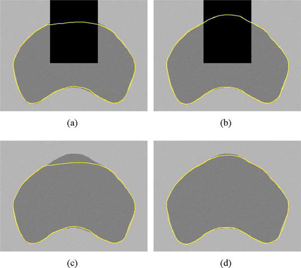
To demonstrate the performance of the proposed PASM method, we first applied the method to segmenting a synthetic TRUS image with a shadow region on the upper part of the prostate. For comparison, the method of using the complete contour for shape prior estimation is also included. As shown in Fig. 7, using PASM was able to get better segmentation result. The reason is that PASM estimates the shape prior in the shadow region completely based on other salient contour parts. Therefore, it will not be influenced by the segmented shape in the shadow region.

Fig. 7.

Segmentation results on a synthetic TRUS image with shadow artifact. (a) Result without using PASM. (b) Result using PASM. (c) and (d) Segmentation results in (a) and (b) imposed on the ground truth image.

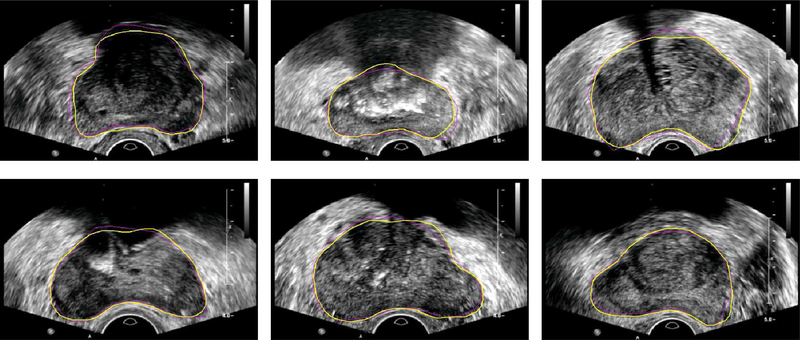
Some example segmentation results of using PASM on real TRUS images are shown in Fig. 8. Compared to the segmentation results on the same images shown in Fig. 4, the segmentation performance has been significantly improved after PASM was applied. The shape model without partial salient contour detection was used in other model-based prostate segmentation methods such as [11] and [13]. Note that the proposed method was applied for segmenting the whole prostate instead of only the midgland region. Segmentation results in the base and the apex regions are shown in Fig. 9.

Fig. 8.

Example segmentation results of the prostate from ultrasound images with shadow areas on top of the prostate. Yellow contours show the automatic segmentation results and the ground truth is shown in magenta.

Fig. 9.

Example segmentation results of the prostate with ground truth in (a) the base and (b) the apex regions.

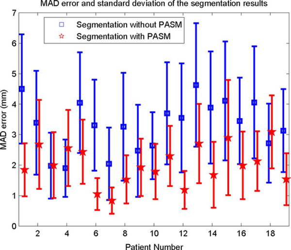
The quantitative evaluation results of the automatic segmentation methods are shown in Fig. 10. It can be seen that the PASM-based method obtained significantly better results (p < 0.05) in almost all the cases compared to the one without PASM. To get an overall quantitative evaluation of the segmentation results over all the patients, the average MAD error was computed by taking the average of the segmentation errors. The average MAD error of the segmentation results using PASM is 2.01 mm ± 1.02 mm over the whole prostate, while the error is 3.30 mm ± 1.55 mm for the segmentation results without using PASM, which was 64.2% improvement.

Fig. 10.

MAD error and standard deviation of the distance between manually and automatically segmented prostate contours.

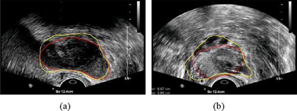
In two of the 19 patients (4 and 18), the PASM-based method did not perform as the method without using PASM, as shown in Fig. 10. Two segmented frames taken from the data are shown in Fig. 11 as an example for illustration. Good performance was obtained by both methods in the midgland of the prostate, which also conforms the results in [11] and [13]. However, in this special case, PASM-based method did not perform well in the area close to the base of the prostate. It can be seen that the boundary between the prostate and the bladder is almost indistinguishable and the upper boundary of the bladder was incorrectly captured by the PASM-based method. On the other hand, the method without using PASM got trapped by the boundaries that happened to be the prostate boundary in this case. Therefore, it performed better. One possible solution to this problem is to model the prostate shape more precisely in different regions, rather than using a global shape model for segmenting the whole prostate, to exclude the irregular shape and the “false” prostate boundary from the segmentation results.

Fig. 11.

Automatic segmentation results of the data from patient 18. Yellow contours show the automatic segmentation results using PASM and the results without using PASM are shown in red. (Left) Image from the middle of the prostate. (Right) Image from the area close to the base of the prostate.

VII. CONCLUSION

In this paper, we demonstrated that missing boundary information in prostate TRUS image can be well estimated from the available partial salient contours. By using the estimated complete shape together with a robust DDM model, the prostate can be automatically segmented from TRUS images with significantly improved results. The study in this paper also features an efficient segmentation algorithm. By using the proposed DDM method, computational complexity has been significantly reduced. The time required for segmenting each image is much shorter than other existing methods.

While the algorithm is very effective for prostate midgland segmentation, its accuracy in the base and apex of the prostate is limited mostly due to the irregular shape of the prostate in those areas and hardly distinguished structure boundaries. The problem will be addressed in our future work. In addition, hardware acceleration will also be explored in the hope to run the algorithm in real-time interventional procedures.

Biography

Pingkun Yan (S’04–M’06) received the B.Eng. degree in electronics engineering and information science from the University of Science and Technology of China, Hefei, China, in 2001, and the Ph.D. degree in electrical and computer engineering from the National University of Singapore, Singapore, in 2006.

He was a Research Associate with the Computer Vision Laboratory, University of Central Florida, Orlando. He is currently a Senior Member of the Research Staff of Philips Research North America, Briarcliff Manor, NY. His research interests include computer vision, pattern recognition, machine learning, and their applications to medical image analysis and image-guided interventions. He is an Associate Editor of the Machine Vision and Applications (Springer).

Dr. Yan was a Program Committee Member of a number of international conferences. He is a full member of the Sigma Xi and a member of the Medical Image Computing and Computer Assisted Intervention Society.

Sheng Xu received the M.S. and Ph.D. degrees in computer science from the Johns Hopkins University, Baltimore, MD.

He is a Senior Member of the Research Staff of Philips Research North America, Briarcliff Manor, NY. His current research interests include surgical navigation, medical image processing, and medical robotics.

Baris Turkbey was born in 1978 in Ankara, Turkey. He received the Medical degree from Hacettepe University School of Medicine, Ankara, in 2003.

For four years, he was a Radiology Resident in the Department of Radiology, Hacettepe University. He is currently a Fellow in the Molecular Imaging Program, National Institutes of Health, Bethesda, MD. His current research interests include genitourinary radiology, molecular imaging, as well as emergency radiology.

Dr. Turkbey is a member of the Radiological Society of North America, the American Roentgen Ray Society, and the Turkish Society of Radiology.

Jochen Kruecker (S’01–M’04) received the Diploma in physics from Rheinische Friedrich-Wilhelms-Universiät, Bonn, Germany, in 1997, and the Ph.D. degree in applied physics from the University of Michigan, Ann Arbor, in 2003.

From 1995 to 1997, he was a Research Assistant with TIMUG e.V., Bonn. During 1997 and 1998, he was with the Ultrasound Group, Basic Radiological Sciences Division, University of Michigan, where he was a Postdoctoral Fellow in the Department of Radiology during 2003 and was engaged in conducting research in ultrasound image registration and breast imaging. During November 2004, he joined Philips Research North America, Briarcliff Manor, NY, where he is currently engaged in the interventional image guidance projects in collaboration with the National Institutes of Health Clinical Center, Bethesda, MD. His research interests include medical image processing and registration, 2-D and 3-D ultrasound imaging, multimodality image fusion, and novel guidance technologies for interventional biopsy and therapy procedures.

REFERENCES

- [1].American Cancer Society. (2008). “Prostate cancer,” American Cancer Society; Atlanta, GA: [Online]. Available: http://www.cancer.org/ [Google Scholar]
- [2].Fichtinger G, Krieger A, Susil RC, Tanács A, Whitcomb LL, and Atalar E, “Transrectal prostate biopsy inside closed MRI scanner with remote actuation, under real-time image guidance,” in Proc. MICCAI (1), 2002, pp. 91–98. [Google Scholar]
- [3].Hodge KK, McNeal JE, Terris MK, and Stamey TA, “Random-systematic versus directed ultrasound-guided core-biopsies of the prostate,” J. Urol, vol. 142, pp. 71–75, 1989. [DOI] [PubMed] [Google Scholar]
- [4].Shen D, Lao Z, Zeng J, Zhang W, Sesterhenn IA, Sun L, Moul JW, Herskovits EH, Fichtinger G, and Davatzikos C, “Optimized prostate biopsy via a statistical atlas of cancer spatial distribution,” Med. Image Anal, vol. 8, pp. 139–150, 2003. [DOI] [PubMed] [Google Scholar]
- [5].Kruecker J, Xu S, Glossop N, Guion P, Choyke P, Singh A, and Wood BJ, “Fusion of real-time transrectal ultrasound with pre-acquired MRI for multimodality prostate imaging,” in Proc. Med. Imag. 2007: Vis., Image-Guid. Procedures Display (SPIE Medical Imaging), vol. 6509, pp. 1201–1212. [Google Scholar]
- [6].Xu S, Kruecker J, Guion P, Glossop N, Neeman Z, Choyke P, Singh AK, and Wood BJ, “Closed-loop control in fused MR-TRUS image-guided prostate biopsy,” in Proc. MICCAI (Lecture Notes in Comput. Sci.), 2007, vol. 4791, pp. 128–135. [DOI] [PMC free article] [PubMed] [Google Scholar]
- [7].Yan P, Xu S, Turkbey B, and Kruecker J, “Optimal search guided by partial active shape model for prostate segmentation in TRUS images,” in Proc. Med. Imag. 2009: Vis., Image-Guid. Procedures Model., Bellingham, WA, vol. 7261, pp. 1G01–1G11. [Google Scholar]
- [8].Shao F, Ling KV, Ng WS, and Wu R, “Prostate boundary detection from ultrasonographic images,” J. Ultrasound Med, vol. 22, pp. 605–623, 2003. [DOI] [PubMed] [Google Scholar]
- [9].Nobel JA and Boukerroui D, “Ultrasound image segmentation: A survey,” IEEE Trans. Med. Imag, vol. 25, no. 8, pp. 987–1010, August. 2006. [DOI] [PubMed] [Google Scholar]
- [10].Badiei S, Salcudean SE, Varah J, and Morris WJ, “Prostate segmentation in 2D ultrasound images using image warping and ellipse fitting,” in Proc. MICCAI, 2006, vol. 4191, pp. 17–24. [DOI] [PubMed] [Google Scholar]
- [11].Ladak HM, Mao F, Wang Y, Downey DB, Steinman DA, and Fenster A, “Prostate boundary segmentation from 2D ultrasound images,” Med. Phys, vol. 27, no. 8, pp. 1777–1788, 2000. [DOI] [PubMed] [Google Scholar]
- [12].Wang Y, Cardinal HN, Downey DB, and Fenster A, “Semiautomatic three-dimensional segmentation of the prostate using two-dimensional ultrasound images,” Med. Phys, vol. 30, pp. 887–897, May 2003. [DOI] [PubMed] [Google Scholar]
- [13].Shen D, Zhan Y, and Davatzikos C, “Segmentation of prostate boundaries from ultrasound images using statistical shape model,” IEEE Trans. Med. Imag, vol. 22, no. 4, pp. 539–551, April. 2003. [DOI] [PubMed] [Google Scholar]
- [14].Zhan Y and Shen D, “Deformable segmentation of 3-D ultrasound prostate images using statistical texture matching method,” IEEE Trans. Med. Imag, vol. 25, no. 3, pp. 256–272, March. 2006. [DOI] [PubMed] [Google Scholar]
- [15].Gong L, Pathak SD, Haynor DR, Cho PS, and Kim Y, “Parametric shape modeling using deformable super ellipses for prostate segmentation,” IEEE Trans. Med. Imag, vol. 23, no. 3, pp. 340–349, March. 2004. [DOI] [PubMed] [Google Scholar]
- [16].Abolmaesumi P and Sirouspour MR, “An interacting multiple model probabilistic data association filter for cavity boundary extraction from ultrasound images,” IEEE Trans. Med. Imag, vol. 23, no. 6, pp. 772–784, June. 2004. [DOI] [PubMed] [Google Scholar]
- [17].Hodge AC, Fenster A, Downey DB, and Ladak HM, “Prostate boundary segmentation from ultrasound images using 2D active shape models: Optimisation and extension to 3D,” Comput. Methods Progr. Biomed, vol. 84, pp. 99–113, 2006. [DOI] [PubMed] [Google Scholar]
- [18].Yan P, Shen W, Kassim AA, and Shah M, “Segmentation of neighboring organs in medical image with model competition,” in Proc. MICCAI (Lecture Notes in Comput. Sci.), 2005, vol. 3749, pp. 270–277. [DOI] [PubMed] [Google Scholar]
- [19].Cootes TF, Taylor CJ, Cooper DH, and Graham J, “Active shape models—Their training and application,” Comput. Vis. Image Understanding, vol. 61, no. 1, pp. 38–59, January. 1995. [Google Scholar]
- [20].Rama JR, Tarrés F, and Eisert P, “Partial PCA in frequency domain,” in Proc. 50th Int. Symp. ELMAR, Zadar, Croatia, September. 2008, vol. 2, pp. 463–466. [Google Scholar]
- [21].Ahn J-H and Oh J-H, “A constrained EM algorithm for principal component analysis,” Neural Comput. no. 15, pp. 57–65, 2003. [DOI] [PubMed] [Google Scholar]
- [22].Skocaj D, Leonardis A, and Bischof H, “Weighted and robust learning of subspace representations,” Pattern Recognit, vol. 40, no. 5, pp. 1556–1569, May 2007. [Google Scholar]
- [23].Tipping ME and Bishop CM, “Probabilistic principal component analysis,” J. R. Statist. Soc., vol. 61, pp. 611–622, 1999. [Google Scholar]
- [24].Williams DJ and Shah M, “A fast algorithm for active contours and curvature estimation,” CVGIP: Image Understanding, vol. 55, no. 1, pp. 14–26, 1992. [Google Scholar]
- [25].Amini AA, Weymouth TE, and Jain RC, “Using dynamic programming for solving variational problems in vision,” IEEE Trans. Pattern Anal. Mach. Intell, vol. 12, no. 9, pp. 855–866, September. 1990. [Google Scholar]
- [26].Bergtholdt M and Schnörr C, “Shape priors and online appearance learning for variational segmentation and object recognition in static scenes,” in Proc. 27th DAGM Symp. Pattern Recognit. (Lecture Notes in Comput. Sci.). Berlin, Germany: Springer-Verlag, 2005, vol. 3663, pp. 342–350. [Google Scholar]
- [27].Burt PJ and Adelson EH, “The Laplacian pyramid as a compact image code,” IEEE Trans. Commun, vol. COM-31, no. 4, pp. 532–540, April. 1983. [Google Scholar]
- [28].Kass M, Witkin A, and Terzopoulos D, “Snakes: Active contour models,” Int. J. Comput. Vis, vol. 1, no. 4, pp. 321–331, 1987. [Google Scholar]
- [29].Ibanez L, Schroeder W, Ng L, and Cates J. (2005). The ITK Software Guide. (2nd ed.). ISBN 1–930934-15–7 [Online]. Available: http://www.itk.org/ItkSoftwareGuide.pdf [Google Scholar]