Near Optimal Linear Algebra in the Online and Sliding Window Models

Abstract

We initiate the study of numerical linear algebra in the sliding window model, where only the most recent W updates in a stream form the underlying data set. Although many existing algorithms in the sliding window model use or borrow elements from the smooth histogram framework (Braverman and Ostrovsky, FOCS 2007), we show that many interesting linear-algebraic problems, including spectral and vector induced matrix norms, generalized regression, and lowrank approximation, are not amenable to this approach in the row-arrival model. To overcome this challenge, we first introduce a unified row-sampling based framework that gives randomized algorithms for spectral approximation, low-rank approximation/projection-cost preservation, and ℓ₁-subspace embeddings in the sliding window model, which often use nearly optimal space and achieve nearly input sparsity runtime. Our algorithms are based on “reverse online” versions of offline sampling distributions such as (ridge) leverage scores, ℓ₁ sensitivities, and Lewis weights to quantify both the importance and the recency of a row; our structural results on these distributions may be of independent interest for future algorithmic design.

Although our techniques initially address numerical linear algebra in the sliding window model, our row-sampling framework rather surprisingly implies connections to the well-studied online model; our structural results also give the first sample optimal (up to lower order terms) online algorithm for low-rank approximation/projection-cost preservation. Using this powerful primitive, we give online algorithms for column/row subset selection and principal component analysis that resolves the main open question of Bhaskara et al. (FOCS 2019). We also give the first online algorithm for ℓ₁-subspace embeddings. We further formalize the connection between the online model and the sliding window model by introducing an additional unified framework for deterministic algorithms using a merge and reduce paradigm and the concept of online coresets, which we define as a weighted subset of rows of the input matrix that can be used to compute a good approximation to some given function on all of its prefixes. Our sampling based algorithms in the row-arrival online model yield online coresets, giving deterministic algorithms for spectral approximation, low-rank approximation/projection-cost preservation, and ℓ_1-subspace embeddings in the sliding window model that use nearly optimal space.

I. Introduction

The advent of big data has reinforced efforts to design and analyze algorithms in the streaming model, where data arrives sequentially, can be observed in a small number of passes (ideally once), and the proposed algorithms are allowed to use space that is sublinear in the size of the input. For example in a typical e-commerce setup, the entries of a row represent the number of each item purchased by a customer in a transaction. As the transaction is completed, the advertiser receives an entire row of information as an update, which corresponds to the row-arrival model. Then the underlying covariance matrix summarizes information about which items tend to be purchased together, while low-rank approximation identifies a representative subset of transactions.

However, the streaming model does not fully address settings where the data is time-sensitive; the advertiser is not interested in the outdated behavior of customers. Thus one scenario that is not well-represented by the streaming model is when recent data is considered more accurate and important than data that arrived prior to a certain time window, as in applications such as network monitoring [8], [9], [18]–[20], event detection in social media [32], and data summarization [11], [25]. To model such settings, Datar et al. [21] introduced the sliding window model, which is parametrized by the size W of the window that represents the size of the active data that we want to analyze, in contrast to the so-called “expired data”. The objective is to compute or approximate statistics only on the active data using memory that is sublinear in the window size W.

The sliding window model is more appropriate than the unbounded streaming model in a number of applications [2], [30], [34], [37]. For example in large scale social media analysis, each row in a matrix can correspond to some online document, such as the content of a Twitter post, and given some corresponding time information. Although a streaming algorithm can analyze the data starting from a certain time, analysis with a recent time frame, e.g., the most recent week or month, could provide much more attractive information to advertisers or content providers. Similarly in the task of data summarization, the underlying data set is a matrix whose rows correspond to a number of subjects, while the columns correspond to a number of features. Information on each subject arrives sequentially and the task is to select a small number of representative subjects, which is usually done through some kind of PCA [33], [35]. However, if the behavior of the subjects has recently and indefinitely changed, we would like the summary to only be representative of the updated behavior, rather than the outdated information.

Another time-sensitive scenario that is not well-represented by the streaming model is when irreversible decisions must be made upon the arrival of each update in the stream, which enables further actions downstream, such as in scheduling, facility location, and data structures. The goal of the online model is to address such settings by requiring immediate and permanent actions on each element of the stream as it arrives, while still remaining competitive with an optimal offline solution that has full knowledge of the entire input. We specifically study the case where the online model must also use space sublinear in the size of the input, though this restriction is not always enforced across algorithms in the online model for other problems. In the context of online PCA, an algorithm receives a stream of input vectors and must immediately project each input vector into a lower dimension space of its choice. The projected vector can then be used as input to some downstream rotationally invariant algorithm, such as classification, clustering, or regression, which would run more efficiently due to the lower dimensional input. Moreover, PCA serves as a popular preprocessing step because it often actually improves the quality of the solution by removing isotropic noise [6] from the data. Thus in applications such as clustering, the denoised projection can perform better than the original input. The online model has also been extensively used in many other applications, such as learning [3], [5], [28], (prophet) secretary problems [24], [26], [36], ad allocation [31], and a variety of graph applications [12], [13], [27].

Generally, the sliding window model and the online model do not seem related, resulting in a different set of techniques being developed for each problem and each setting. Surprisingly, our results exhibit a seemingly unexplored and interesting connection between the sliding window model and the online model. Our observation is that an online algorithm should be correct on all prefixes of the input, in case the stream terminates at that prefix; on the other hand, a sliding window algorithm should be correct on all suffixes of the input, in case the previous elements expire leaving only the suffix (and perhaps a bunch of “dummy” elements). Then can we gain something by viewing each update to a sliding window algorithm as an update to an online algorithm in reverse? At first glance, the answer might seem to be no; we cannot simulate an online algorithm with the stream in reverse order because it would have access to the entire stream whereas a sliding window algorithm only maintains a sketch of the previous elements upon each update. However, it turns out that in the row-arrival model, a sketch of the previous elements often suffices to approximately simulate the entire stream input to the online algorithm. Indeed, we show that any row-sampling based online algorithm for the problems of spectral approximation, low-rank approximation/projection-cost preservation, and ℓ₁-subspace embedding automatically implies a corresponding deterministic sliding window algorithm for the problem!

A. Our Contributions

We initiate and perform a comprehensive study for both randomized and deterministic algorithms in the sliding window model. We first present a randomized row sampling framework for spectral approximation, low-rank approximation/projection-cost preservation, and ℓ₁-subspace embeddings in the sliding window model. Most of our results are space or time optimal, up to lower order terms. Our sliding window structural results imply structural results for the online setting, which we use to give algorithms for row/column subset selection, PCA, projection-cost preservation, and subspace embeddings in the online model. Our online algorithms are simple and intuitive, yet they either are novel for the particular problem or improve upon the state-of-the-art, e.g., Bhaskara et al.(FOCS 2019) [4]. Finally, we formalize a surprising connection between online algorithms and sliding window algorithms by describing a unified framework for deterministic algorithms in the sliding window model based on the merge-and-reduce paradigm and the concept of online coresets, which are provably generated by online algorithms.

Row Sampling Framework for the Sliding Window Model:

One may ask whether existing algorithms in the sliding window model can be generalized to problems for numerical linear algebra. In the full version of the paper [7], we give counterexamples showing that various linear-algebraic functions, including the spectral norm, vector induced matrix norms, generalized regression, and low-rank approximation, are not smooth according to the definitions of [10] and therefore cannot be used in the smooth histogram framework. This motivates the need for new frameworks for problems of linear algebra in the sliding window model. We first give a row sampling based framework for space and runtime efficient randomized algorithms for numerical linear algebra in the sliding window model.

Framework I.1 (Row Sampling Framework for the Sliding Window Model).

There exists a row sampling based framework in the sliding window model that upon the arrival of each new row of the stream with condition number κ chooses whether to keep or discard each previously stored row, according to some predefined probability distribution for each problem. Using the appropriate probability distribution, we obtain for any approximation parameter ε > 0:

1. A randomized algorithm for spectral approximation in the sliding window model that with high probability, outputs a matrix M that is a subset of (rescaled) rows of an input matrix $A\in {ℝ}^{W\times d}$ such that (1 − ε) A^⊤A ⪯ M^⊤M ⪯ (1 + ε) A^⊤A, while storing $\mathcal{O}\left(\frac{d}{{\epsilon }^2}\text{ log }n\text{ log }\kappa \right)$ rows at any time and using nearly input sparsity time. (See Theorem II.4.)

2. A randomized algorithm for low-rank approximation/projection-cost preservation in the sliding window model that with high probability, outputs a matrix M that is a subset of (rescaled) rows of an input matrix $A\in {ℝ}^{W\times d}$ such that for all rank k orthogonal projection matrices $P\in {ℝ}^{d\times d}$,

   $$\Vert M-MP{\Vert }_F^2\in (1\pm \epsilon )\Vert A-AP{\Vert }_F^2,$$

   while storing $\mathcal{O}\left(\frac{k}{{\epsilon }^2}\text{ log }n{\text{ log}}^2\kappa \right)$ rows at any time and using nearly input sparsity time. (See Theorem II.10.)

3. A randomized algorithm for ℓ₁-subspace embeddings in the sliding window model that with high probability, outputs a matrix M that is a subset of (rescaled) rows of an input matrix $A\in {ℝ}^{W\times d}$ such that (1 − ε) ∥Ax∥₁ ≤ ∥Mx∥₁ ≤ (1 + ε) ∥Ax∥₁ for all $x\in {ℝ}^d$, while storing $\mathcal{O}\left(\frac{d^2}{{\epsilon }^2}{\text{ log}}^{2}n\text{ log }\kappa \right)$ rows at any time. (See Theorem IV.5.)

Here we say the stream has condition number κ if the ratio of the largest to smallest nonzero singular values of any matrix formed by consecutive rows of the stream is at most κ.

For low-rank approximation/projection-cost preservation, we can further improve the polylogarithmic factors from $\mathcal{O}\left(\frac{k}{{\epsilon }^2}\text{ log }n{\text{ log}}^2\kappa \right)$ rows stored at any time to $\mathcal{O}\left(\frac{k}{{\epsilon }^2}{\text{ log}}^{2}n\right)$, under the assumption that the entries of the underlying matrix are integers with magnitude at most poly(n) even though log κ can be as large as $\mathcal{O}(d\text{ log }n)$ with these assumptions. To the best of our knowledge, not only are our contributions in Framework I.1 the first such algorithms for these problems in the sliding window model, but also Theorem II.4 and Theorem II.10 are both space and runtime optimal up to lower order terms, even compared to row sampling algorithms in the offline setting for most reasonable regime of parameters [1], [23].

Numerical Linear Algebra in the Online Model:

An important step in the analysis of our row sampling framework for numerical linear algebra in the sliding window model is bounding the sum of the sampling probabilities for each row. In particular, we provide a tight bound on the sum of the online ridge leverage scores that was previously unexplored. We show that our bounds along with the paradigm of row sampling with respect to online ridge leverage scores offer simple online algorithms that improve upon the state-of-the-art across broad applications.

Theorem I.2 (Online Rank k Projection-Cost Preservation).

Given parameters ε > 0, k > 0, and a matrix $A\in {ℝ}^{n\times d}$, whose rows a₁, … , a_n arrive sequentially in a stream with condition number κ, there exists an online algorithm that with high probability, outputs a matrix M that has $\mathcal{O}\left(\frac{k}{{\epsilon }^2}\text{ log }n{\text{ log}}^2\kappa \right)$ (rescaled) rows of A and for all rank k orthogonal projection matrices $P\in {ℝ}^{d\times d}$,

$$(1-\epsilon )\Vert A-AP{\Vert }_F^2\le \Vert M-MP{\Vert }_F^2\le (1+\epsilon )\Vert A-AP{\Vert }_F^2.$$

(See Theorem III.1.)

Theorem III.1 immediately yields improvements on the two online algorithms recently developed by Bhaskara et al. (FOCS 2019) for online row subset selection and online PCA [4].

Theorem I.3 (Online Row Subset Selection).

Given parameters ε > 0, k > 0, and a matrix $A\in {ℝ}^{n\times d}$, whose rows a₁, … , a_n arrive sequentially in a stream with condition number κ, there exists an online algorithm that with high probability, outputs a matrix M with $\mathcal{O}\left(\frac{k}{\epsilon }\text{ log }n{\text{ log}}^2\kappa \right)$ rows that contains a matrix T of k rows such that

$${\Vert A-A{T}^{-1}T\Vert }_F^2\le (1+\epsilon ){\Vert A-A_{(k)}\Vert }_F^2.$$

(See Theorem III.2.)

By comparison, the online row subset selection algorithm of [4] stores $\mathcal{O}\left(\frac{k}{{\epsilon }^2}\text{ log }n{\text{ log}}^2\kappa \right)$ rows to succeed with high probability. Moreover, our algorithm provides the guarantee of the existence of a subset T of k rows that provides a (1 + ε)-approximation to the best rank k solution, whereas [4] promises the bicriteria result that their matrix with rank $\mathcal{O}\left(\frac{k}{{\epsilon }^2}\text{ log }n{\text{ log}}^2\kappa \right)$ is a (1 + ε)-approximation to the best rank k solution.

The online PCA algorithm of [4] also offers this bicriteria guarantee; for an input matrix $A\in {ℝ}^{n\times d}$, they give an algorithm that outputs a matrix $M\in {ℝ}^{n\times m}$, where $m=\mathcal{O}\left(\frac{k}{{\epsilon }^2}{(\text{ log }n+\text{ log }\kappa )}^4\right)$ and a matrix X of rank m, so that $\Vert A-MX{\Vert }_F^2\le (1+\epsilon ){\Vert A-A_{(k)}\Vert }_F^2$. Our online row subset selection can also be adjoined with the online PCA algorithm of [4] to offer the promise of the existence of a submatrix $Y\in {ℝ}^{k\times d}$ within X such that there exists a matrix B with $\Vert A-BY{\Vert }_F^2\le (1+\epsilon ){\Vert A-A_{(k)}\Vert }_F^2$.

Theorem I.4 (Online Principal Component Analysis).

Given parameters n, d, k, ε > 0 and a matrix $A\in {ℝ}^{n\times d}$ whose rows arrive sequentially in a stream with condition number κ, let $m=\mathcal{O}\left(\frac{k}{{\epsilon }^2}{(\text{ log }n+\text{ log }\kappa )}^4\right)$. There exists an algorithm for online PCA that immediately outputs a row $m_i\in {ℝ}^m$ after seeing row $a_i\in {ℝ}^d$ and with high probability, outputs a matrix $X\in {ℝ}^{m\times d}$ at the end of the stream such that

$$\Vert A-MX{\Vert }_F^2\le (1+\epsilon ){\Vert A-A_{(k)}\Vert }_F^2,$$

where A_(k) is the best rank k approximation to A. Moreover, X contains a submatrix $Y\in {ℝ}^{k\times d}$ such that there exists a matrix B such that

$$\Vert A-BY{\Vert }_F^2\le (1+\epsilon ){\Vert A-A_{(k)}\Vert }_F^2.$$

(See Theorem III.3.)

Our sliding window algorithm for ℓ₁-subspace embeddings also uses an online ℓ₁-subspace embedding algorithm that we develop.

Theorem I.5 (Online ℓ₁-Subspace Embedding).

Given $\epsilon >\frac{1}{n}$ and a matrix $A\in {ℝ}^{n\times d}$, whose rows a₁, … , a_n arrive sequentially in a stream with condition number κ, there exists an online algorithm that outputs a matrix M with $\mathcal{O}\left(\frac{d^2}{{\epsilon }^2}{\text{ log}}^{2}n\text{ log }\kappa \right)$ (rescaled) rows of A such that

$$(1-\epsilon )\Vert Ax{\Vert }_1\le \Vert Mx{\Vert }_1\le (1+\epsilon )\Vert Ax{\Vert }_1,$$

for all $x\in {ℝ}^d$ with high probability. (See Theorem IV.4.)

A Coreset Framework for Deterministic Sliding Window Algorithms:

To formalize a connection between online algorithms and sliding window algorithms, we give a framework for deterministic sliding window algorithms based on the merge-and-reduce paradigm and the concept of an online coreset, which we define as a weighted subset of rows of A that can be used to compute a good approximation to some given function on all prefixes of A. On the other hand, observe that a row-sampling based online algorithm does not know when the input might terminate, so it must output a good approximation to any prefix of the input, which is exactly the requirement of an online coreset! Moreover, an online cannot revoke any of its decisions, so the history of its decisions are fully observable. Indeed, each of our online algorithms imply the existence of an online coreset for the corresponding problem.

Framework I.6 (Coreset Framework for Deterministic Sliding Window Algorithms).

There exists a merge-and-reduce framework for numerical linear algebra in the sliding window model using online coresets. If the input stream has condition number κ, then for approximation parameter $\epsilon >\frac{1}{n}$, the framework gives:

1. A deterministic algorithm for spectral approximation in the sliding window model that outputs a matrix M that is a subset of (rescaled) rows of an input matrix $A\in {ℝ}^{w\times d}$ such that (1 − ε) A^⊤A ⪯ M^⊤M ⪯ (1 + ε) A^⊤A, while storing $\mathcal{O}\left(\frac{d}{{\epsilon }^2}{\text{ log}}^{4}n\text{ log }\kappa \right)$ rows at any time. (See Theorem V.5).

2. A deterministic algorithm for low-rank approximation/projection-cost preservation in the sliding window model that outputs a matrix M that is a subset of (rescaled) rows of an input matrix $A\in {ℝ}^{W\times d}$ such that for all rank k orthogonal projection matrices $P\in {ℝ}^{d\times d}$,

   $$\Vert M-MP{\Vert }_F^2\in (1\pm \epsilon )\Vert A-AP{\Vert }_F^2,$$

   while storing $\mathcal{O}\left(\frac{k}{{\epsilon }^2}{\text{ log}}^{4}n{\text{ log}}^2\kappa \right)$ rows at any time. (See Theorem V.7.)

3. A deterministic algorithm for ℓ₁-subspace embeddings in the sliding window model that outputs a matrix M that is a subset of (rescaled) rows of an input matrix $A\in {ℝ}^{W\times d}$ such that (1 − ε) ∥Ax∥₁ ≤ ∥Mx∥₁ ≤ (1 + ε) ∥Ax∥₁ for all $x\in {ℝ}^d$, while storing $\mathcal{O}\left(\frac{d}{{\epsilon }^2}{\text{ log}}^{5}n\text{ log }\kappa \right)$ rows at any time. (See Theorem V.11).

All of the results presented using Framework I.6 are space optimal, up to lower order terms [1], [17], [23]. Again we have the property for low-rank approximation/projection-cost preservation that the number of sampled rows can be improved from $\mathcal{O}\left(\frac{k}{{\epsilon }^2}\text{ log }n{\text{ log}}^2\kappa \right)$ to $\mathcal{O}\left(\frac{k}{{\epsilon }^2}{\text{ log}}^{2}n\right)$, under the assumption that the entries of the underlying matrix are integers at most poly(n) in magnitude.

We remark that neither our randomized framework Framework I.1 nor our deterministic framework Framework I.6 requires the sliding window parameter W as input during the processing of the stream. Instead, they create oblivious data structures from which approximations for any window can be computed after processing the stream. We outline our methods in this extended abstract and defer all proofs to [7].

II. Row Sampling Framework for the Sliding Window Model

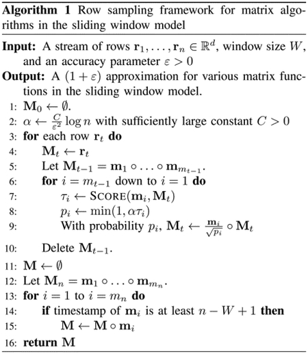
In this section, we give space and time efficient algorithms for matrix functions in the sliding window model. Our general approach will be to use the following framework. As the stream $r_1,\dots ,r_n\in {ℝ}^d$ arrives, we shall maintain a weighted subset of these rows at each time. Suppose at some time t, we have a matrix $M_t=r_{t,1}○\dots ○r_{t,m_t}$ of weighted rows of the stream that can be used to give a good approximation to the function applied to any suffix of the stream. Upon the arrival of row t + 1, we first set M_t+1 = r_t+1. Then starting with i = m_t and moving backwards toward i = 1, we repeatedly prepend a weighted version of r_t,i to M_t+1 with some probability that depends on r_t,i, M_t+1, and the matrix function to be approximated. Once the rows of M_t have each been either added to M_t+1 or discarded, we proceed to row t + 2, i.e., the next update in the stream.

Note that the matrices M_t serve no real purpose other than for presentation; the framework is just storing a subset of weighted rows at each time and repeatedly performing online row sampling, starting with the most recent row. Since an online algorithm must be correct on all prefixes of the input, then our framework must be correct on all suffixes of the input and in particular, on the sliding window. This observation demonstrates a connection between online algorithms and sliding window algorithms that we explore in greater detail in future sections. We give our framework in Algorithm 1.

A. ℓ₂-Subspace Embedding

We first give a randomized algorithm for spectral approximation in the sliding window model that is both space and time efficient. [16] defined the concept of online (ridge) leverage scores and show that by sampling each row of a matrix A with probability proportional to its online leverage score, the weighted sample at the end of the stream provides a (1 + ε) spectral approximation to A. We recall the definition of online ridge leverage scores of a matrix from [16], as well as introduce reverse online ridge leverage scores.

Definition II.1 (Online/Reverse Online (Ridge) Leverage Scores).

For a matrix $A=a_1○\dots ○a_n\in {ℝ}^{n\times d}$, let A_i = a₁ ○ … ○ a_i and Z_i = a_n ○ … ○ a_i. Let λ ≥ 0. The online λ-ridge leverage score of row a_i is defined to be $\text{min}\left(1,a_i{\left(A_{i-1}^{\top }{A}_{i-1}+\lambda \mathbb{I}\right)}^{-1}{a}_i^{\top }\right)$, while the reverse online λ-ridge leverage score of row a_i is defined to be $\text{min}\left(1,a_i{\left(Z_{i+1}^{\top }{Z}_{i+1}+\lambda \mathbb{I}\right)}^{-1}{a}_i^{\top }\right)$. The (reverse) online leverage scores are defined respectively by setting λ = 0, though we use the convention that if the (reverse) online leverage score of a_i is 1 if rank(A_i) > rank(A_i−1) (respectively if rank(Z_i) > rank(Z_i+1)).

From the definition, it is evident that the reverse online (ridge) leverage scores are monotonic; whenever a new row is added to A, the scores of existing rows cannot increase.

Intuitively, the online leverage score quantifies how important row a_i is, with respect to the previous rows, while the reverse online leverage score quantifies how important row a_i is, with respect to the following rows, and the ridge leverage scores are regularized versions of these quantities. As the name suggests, online (ridge) leverage scores seem appropriate for online algorithms while reverse online (ridge) leverage scores seem appropriate for sliding window algorithms, where recency is an emphasis. Hence, we use reverse online leverage scores in computing the sampling probability of each particular row in Algorithm 2 that serves as our customized Score function in Algorithm 1 for spectral approximation.

However, these quantities are related; [16] provide an asymptotic bound on the sum of the online ridge leverage scores of any matrix, which also implies a bound on the sum of the reverse online ridge leverage scores, by reversing the order of the rows in a matrix. We present these results for the case where the input matrix has full rank, noting that similar bounds can be provided if the input matrix is not full rank by replacing the smallest singular value with the smallest nonzero singular value.

Lemma II.2 (Bound on Sum of Online Ridge Leverage Scores).

[16] Let the rows of $A=a_1○\dots ○a_n\in {ℝ}^{n\times d}$ arrive in a stream with condition number κ and let ℓ_i be the online (ridge) leverage score of a_i with regularization λ. Then ${\sum }_{i=1}^n{\mathcal{l}}_i=\mathcal{O}\left(d\text{ log }\frac{\Vert A{\Vert }_2}{\lambda }\right)$ for λ > σ_min(A) and ${\sum }_{i=1}^n{\mathcal{l}}_i=\mathcal{O}(d\text{ log }\kappa )$ for λ ≤ σ_min(A). It follows that if τ_i is the reverse online ridge leverage score of a_i, then ${\sum }_{i=1}^n{\tau }_i=\mathcal{O}\left(d\text{ log }\frac{\Vert A{\Vert }_2}{\lambda }\right)$ for λ > σ_min(A) and ${\sum }_{i=1}^n{\tau }_i=\mathcal{O}(d\text{ log }\kappa )$ for λ ≤ σ_min(A).

We show that at any time t, Algorithm 1 using the Score function of Algorithm 2 stores a matrix M_t whose rows with timestamp after a time i ∈ [t] provides a (1 + ε) spectral approximation to any matrix Z_i = r_t○…○r_i. This statement shows a good approximation to any suffix of the stream at all times and in particular for t = n and i = n − W + 1, shows that Algorithm 1 using the Score function of Algorithm 2 outputs a spectral approximation for the matrix induced by the sliding window model.

Lemma II.3 (Spectral Approximation Guarantee, Bounds on Sampling Probabilities).

Let t ∈ [n], λ ≥ 0 and ε > 0. For i ∈ [t], let $q_i=\text{min}\left(1,\alpha \cdot r_i{\left(Z_{i+1}\top Z_{i+1}\right)}^{-1}{r}_i^{\top }\right)$, where Z_i+1 = r_t ○ … ○ r_i+1. Then with high probability after the arrival of row r_t, Algorithm 1 using the Score function of Algorithm 2 will have sampled each row r_i with probability at least q_i and probability at most 4q_i. Moreover, if Y is the suffix of M_t consisting of the (scaled) rows whose timestamps are at least i, then

$$(1-\epsilon )\left(Z_i^{\top }{Z}_i+\lambda \mathbb{I}\right)⪯Y^{\top }Y+\lambda \mathbb{I}⪯(1+\epsilon )\left(Z_i^{\top }{Z}_i+\lambda \mathbb{I}\right).$$

Theorem II.4 (Randomized Spectral Approximation Sliding Window Algorithm).

Let $r_1,\dots ,r_n\in {ℝ}^d$ be a stream of rows and κ be the condition number of the stream. Let W > 0 be a window size parameter and A = r_n−W+1 ○ … ○ r_n be the matrix consisting of the W most recent rows. Given a parameter ε > 0, there exists an algorithm that outputs a matrix M with a subset of (rescaled) rows of A such that (1 − ε) A^⊤A ⪯ M^⊤M ⪯ (1 + ε) A^⊤A and stores $\mathcal{O}\left(\frac{d}{{\epsilon }^2}\text{ log }n\text{ log }\kappa \right)$ rows at any time, with high probability.

B. Low-Rank Approximation

In this section, we give a randomized algorithm for low-rank approximation in the sliding window model that is both space and time optimal, up to lower order terms. Throughout this section, we use A_(k) to denote the best rank k approximation to a matrix $A\in {ℝ}^{n\times d}$ so that $A_{(k)}:={\text{argmin}}_{\text{rank}(X)\le k}\Vert A-X{\Vert }_F^2$ . Recall the following definition of a projection-cost preservation, from which it follows that obtaining a projection-cost preservation of A suffices to produce a low-rank approximation of A.

Definition II.5 (Rank k Projection-Cost Preservation [15]).

For m < n, a matrix $M\in {ℝ}^{m\times d}$ of rescaled rows of $A\in {ℝ}^{n\times d}$ is a (1 + ε) projection-cost preservation if, for all rank k orthogonal projection matrices $P\in {ℝ}^{d\times d}$,

$$(1-\epsilon )\Vert A-AP{\Vert }_F^2\le \Vert M-MP{\Vert }_F^2\le (1+\epsilon )\Vert A-AP{\Vert }_F^2.$$

[15] showed that an additive-multiplicative spectral approximation of a matrix A along with an additional moderate condition that holds for ridge leverage score sampling gives a projection-cost preservation of A.

Lemma II.6.

[15] Let $A=a_1○\dots ○a_n\in {ℝ}^{n\times d}$ and $\lambda \le \frac{{\Vert A-A_{(k)}\Vert }_F^2}{k}$. Let p be the largest integer such that σ_p(A)² ≥ λ and let X = A − A_(p). Let $S\in {ℝ}^{m\times n}$ be a sampling matrix so that M = AS is a subset of scaled rows of A. If $(1-\epsilon )\left(A^{\top }A+\lambda \mathbb{I}\right)\underset{\_}{\prec }{M}^{\top }M+\lambda \mathbb{I}⪯(1+\epsilon )(A^{\top }A+\lambda \mathbb{I})$ and $\left|\Vert SX{\Vert }_F^2-\Vert X{\Vert }_F^2\right|\le \epsilon {\Vert A-A_{(k)}\Vert }_F^2$, then M is a rank k projection-cost preservation of A with approximation parameter 24ε.

We focus our discussion on the additive-multiplicatve spectral approximation since the same argument of [15] with Freedman’s inequality rather than Chernoff bounds shows sampling matrices generated from ridge leverage scores satisfy the condition $\left|\Vert SX{\Vert }_F^2-\Vert X{\Vert }_F^2\right|\le \epsilon {\Vert A-A_{(k)}\Vert }_F^2$ with high probability, even when the entries of S are not independent:

Lemma II.7.

[15] Let $A=a_1○\dots ○a_n\in {ℝ}^{n\times d}$, $\lambda =\frac{{\Vert A-A_{(k)}\Vert }_F^2}{k}$, and τ_i be the ridge leverage score of a_i with regularization λ. Let p be the largest integer such that σ_p(A)² ≥ λ and let X = A − A_(p). Let $S\in {ℝ}^{m\times n}$ be a sampling matrix so that row a_i is sampled by S, not necessarily independently, with probability at least $\text{min}\left(1,\frac{C{\tau }_i}{{\epsilon }^2}\text{ log }n\right)$ for sufficiently large constant C. Then $\left|\Vert SX{\Vert }_F^2-\Vert X{\Vert }_F^2\right|\le \epsilon {\Vert A-A_{(k)}\Vert }_F^2$ with high probability.

On the other hand, our space analysis in Section II-A relied on bounding the sum of the online leverage scores by $\mathcal{O}(d\text{ log }\kappa )$ through Lemma II.2; a better bound is not known if we set $\lambda =\frac{{\Vert A-A_{(k)}\Vert }_F^2}{k}$. This gap provides a barrier for algorithmic design not only in the sliding window model but also in the online model. We show a tighter analysis showing that the sum of the online ridge leverage scores for $\lambda =\frac{{\Vert A-A_{(k)}\Vert }_F^2}{k}$ is $\mathcal{O}(k\text{ log }\kappa )$.

Now if we knew the value of $\frac{{\Vert A-A_{(k)}\Vert }_F^2}{k}$ a priori, we could set $\lambda \le \frac{{\Vert A-A_{(k)}\Vert }_F^2}{k}$ and immediately apply Lemma II.3 to show that the output of Algorithm 1 with a SCORE function that uses the λ regularization outputs a matrix M that is a rank k projection-cost preservation of A.

Initially, even a constant factor approximation to $\frac{{\Vert A-A_{(k)}\Vert }_F^2}{k}$ seems challenging because the quantity is not smooth. This issue can be circumvented using additional procedures, such as spectral approximation on rows with reduced dimension [14]. Even simpler, observe that sampling with any regularization factor $\lambda <\frac{{\Vert A-A_{(k)}\Vert }_F^2}{k}$ would still provide the guarantees of Lemma II.6.

We could set λ = 0 and still obtain a rank k projection-cost preservation of A, but smaller values of λ correspond to larger number of sampled rows and the total number of sampled rows for λ = 0 would be proportional to d, as opposed to our goal of k. Instead, observe that if B is any prefix or suffix of rows of A, then ${\Vert B-B_{(k)}\Vert }_F^2\le {\Vert A-A_{(k)}\Vert }_F^2$. In other words, we can use the rows that have already been sampled to give a constant factor approximation to ${\Vert A-A_{(k)}\Vert }_F^2$ as it evolves, i.e., as more rows of A arrive. We again pay for the underestimate to ${\Vert A-A_{(k)}\Vert }_F^2$ by sampling an additional number of rows, but we show that we cannot sample too many rows before our approximation to ${\Vert A-A_{(k)}\Vert }_F^2$ doubles, which only incurs an additional $\mathcal{O}(\text{ log }\kappa )$ factor in the number of sampled rows. We give the Score function for low-rank approximation in Algorithm 3.

We first bound the probability that each row is sampled, analogous to Lemma II.3.

Lemma II.8 (Projection-Cost Preservation Guarantee, Bounds on Sampling Probabilities).

Let t ∈ [n] be fixed and for each i ∈ [t], let Z_i = r_t ○ … ○ r_i. Let $\lambda =\frac{{\Vert Z_{i+1}-{\left(Z_{i+1}\right)}_{(k)}\Vert }_F^2}{k}$ and ε > 0. Let $r_i{\left(Z_{i+1}\top Z_{i+1}+\lambda \mathbb{I}\right)}^{-1}{r}_i^{\top })$. Then with high probability after the arrival of row r_t, Algorithm 1 using the Score function of Algorithm 3 will have sampled row r_i with probability at least q_i and probability at most 2q_i. Moreover, if Y is the suffix of M_t consisting of the (scaled) rows whose timestamps are at least i, then

$$(1-\epsilon )\left(Z_i^{\top }{Z}_i+\lambda \mathbb{I}\right)⪯Y^{\top }Y+\lambda \mathbb{I}⪯(1+\epsilon )\left(Z_i^{\top }{Z}_i+\lambda \mathbb{I}\right).$$

We now give a tighter bound on the sum of the online λ-ridge leverage scores l_i for $\lambda =\frac{{\Vert A-A_{(k)}\Vert }_2^2}{k}$.

Lemma II.9 (Bound on Sum of Online Ridge Leverage Scores).

Let $A\in {ℝ}^{n\times d}$ have condition number κ. Let β ≥ 1, k ≥ 1 be constants and $\lambda =\frac{{\Vert A-A_{(k)}\Vert }_2^2}{\beta k}$. Then ${\sum }_{i=1}^n{l}_i=\mathcal{O}(k\text{ log }\kappa )$.

The sum of the reverse online λ-ridge leverage scores is bounded by the same quantity, since the rows of the input matrix can simply be considered in reverse order. We now show that Algorithm 1 using the Score function of Algorithm 3 gives a relative error low-rank approximation with efficient space usage.

Theorem II.10 (Randomized Low-Rank Approximation Sliding Window Algorithm).

Let $r_1,\dots ,r_n\in {ℝ}^d$ be a stream of rows and κ be the condition number of the matrix r₁ ○ …. ○ r_n. Let W > 0 be a window size parameter and A = r_n−W+1 ○ …. ○ r_n be the matrix consisting of the W most recent rows. Given a parameter ε > 0, there exists an algorithm that with high probability, outputs a matrix M that is a (1 + ε) rank k projection-cost preservation of A and stores $\mathcal{O}\left(\frac{k}{{\epsilon }^2}\text{ log }n{\text{ log}}^2\kappa \right)$ rows at any time.

We describe how to achieve nearly input sparsity runtime and elaborate on bounded precision and condition number in [7].

III. Simple Rank Constrained Algorithms in the Online Model

In this section, we show that the paradigm of row sampling with respect to online ridge leverage scores offers simple analysis for a number of online algorithms that improve upon the state-of-the-art.

A. Online Projection-Cost Preservation

As a warm-up, we first demonstrate how our previous analysis bounding the sum of the online ridge leverage scores can be applied to analyze a natural online algorithm for producing a projection-cost preservation of a matrix $A=a_1○\dots ○a_n\in {ℝ}^{n\times d}$. Our algorithm samples each row with probability equal to the online ridge leverage scores, where the regularization parameter λ_i is computed at each step. Note that if A_i = a₁ ○ …. ○ a_i, then ${\Vert A_i-{\left(A_i\right)}_{(k)}\Vert }_F^2\le {\Vert A_j-{\left(A_j\right)}_{(k)}\Vert }_F^2$ for any i < j. Thus if ${\lambda }_i=\frac{{\Vert A_{i-1}-{\left(A_{i-1}\right)}_{(k)}\Vert }_F^2}{k}$, then sampling row a_i with online ridge leverage score regularized by λ_i has a higher probability than with ridge leverage score regularized by $\lambda =\frac{{\Vert A-A_{(k)}\Vert }_F^2}{k}$. Although [16] was only interested in spectral approximation and therefore set λ = εσ_min(A), they nevertheless shows that online row sampling with any regularization λ gives an additive-multiplicative spectral approximation to A. Thus by setting $\lambda =\frac{{\Vert A-A_{(k)}\Vert }_F^2}{k}$, our algorithm outputs a rank k projection-cost preservation of A by Lemma II.6 and Lemma II.7. Moreover, our bounds for the sum of the online ridge leverage scores in Lemma II.9 show that our algorithm only samples a small number of rows, optimal up to lower order factors.

Theorem III.1 (Online Rank k Projection-Cost Preservation).

Given parameters ε > 0, k > 0, and a matrix $A\in {ℝ}^{n\times d}$ whose rows a₁, … , a_n arrive sequentially in a stream with condition number κ, there exists an online algorithm that outputs a matrix M with $\mathcal{O}\left(\frac{k}{{\epsilon }^2}\text{ log }n{\text{ log}}^2\kappa \right)$ (rescaled) rows of A such that

$${\Vert M-M_{(k)}\Vert }_F^2\in (1\pm \epsilon ){\Vert A-A_{(k)}\Vert }_F^2,$$

and thus M is a rank k projection-cost preservation of A, with high probability.

B. Online Row Subset Selection

We next describe how to perform row subset selection in the online model. Our starting point is an offline algorithm by [15] and the paradigm of adaptive sampling [22], [23], [29], which is the procedure of repeatedly sampling rows of A with probability proportional to their squared distances to the subspace spanned by Z. [15] first obtained a matrix Z that is a constant factor low-rank approximation to the underlying matrix A through ridge-leverage score sampling. They observed that a theorem by [22] shows that adaptive sampling $\mathcal{O}\left(\frac{k}{\epsilon }\right)$ additional rows S of A against the rows of Z suffices for Z∪S to contain a (1 + ε) factor approximation to the online row subset selection problem.

[15] then adapted this approach to the streaming model by maintaining a reservoir of $\mathcal{O}\left(\frac{k}{\epsilon }\right)$ rows and replacing rows appropriately as new rows arrive and more information about Z is obtained. Alternatively, we modify the proof of [22] if Z is given to show that adaptive sampling can also be performed on data streams to obtain a different but valid S by oversampling each row of A by a $\mathcal{O}\left(\frac{k}{\epsilon }\right)$ factor. Moreover by running a low-rank approximation algorithm in parallel, downsampling can be performed as rows of Z arrive, so that the above approach can be performed in one stream.

In the online model, we cannot downsample rows of S once they are selected, since Z evolves as the stream arrives. Fortunately, [15] showed that the adaptive sampling probabilities can be upper bounded by the λ-ridge leverage scores, where $\lambda =\frac{1}{k}{\Vert A-A_{(k)}\Vert }_F^2$. Since the λ-ridge leverage scores are at most the online λ-ridge leverage scores, we can again sample rows proportional to their online λ-ridge leverage scores. It then suffices to again use Lemma II.9 to bound the number of rows sampled in this manner.

Theorem III.2 (Online Row Subset Selection).

Given parameters $0<\epsilon <\frac{1}{2}$, k > 0 and a matrix $A\in {ℝ}^{n\times d}$ whose rows a₁, … , a_n arrive sequentially in a stream with condition number κ, there exists an online algorithm that with high probability, outputs a matrix M with $\mathcal{O}\left(\frac{k}{\epsilon }\text{ log }n{\text{ log}}^2\kappa \right)$ rows that contains a matrix T of k rows such that

$${\Vert A-A{T}^{-1}T\Vert }_F^2\le (1+\epsilon ){\Vert A-A_{(k)}\Vert }_F^2.$$

C. Online Principal Component Analysis

Recall that in the online PCA problem, rows of the matrix $A=a_1○\dots ○a_n\in {ℝ}^{n\times d}$ arrive sequentially in a data stream and after each row a_i arrives, the goal is to immediately output a row $m_i\in {ℝ}^{1\times m}$ such that at the end of the stream, there exists a low-rank matrix $X\in {ℝ}^{m\times d}$ such that

$$\Vert A-MX{\Vert }_F^2\le (1+\epsilon ){\Vert A-A_{(k)}\Vert }_F^2,$$

where M = m₁ ○ … ○ m_n and A_(k) is again the best rank k approximation to A.

[4] gave an algorithm for the online PCA problem that embeds into a matrix X that has rank $\mathcal{O}\left(\frac{k}{{\epsilon }^2}{(\text{ log }n+\text{ log }\kappa )}^4\right)$ with high probability, where κ is the condition number of A. Their algorithm maintains and updates the matrix X throughout the data stream. After the arrival of row a_i, the matrix X is updated using a combination of residual based sampling and a black-box theorem of [6]. Row m_i is then output as the embedding of a_i into X by m_i = a_iX⁽ⁱ⁾, where X⁽ⁱ⁾ is the matrix X after row i has been processed by X. X has the property that no rows from X are ever removed across the duration of the algorithm, so then m_i is only an upper bound on the best embedding of a_i. However, this matrix X does not provably contain a good rank k approximation to A. That is, X does not contain a rank k submatrix $Y\in {ℝ}^{k\times d}$ such that there exists a matrix B such that

$$\Vert A-BY{\Vert }_F^2\le (1+\epsilon ){\Vert A-A_{(k)}\Vert }_F^2.$$

Recall that our online row subset selection algorithm returns a matrix $Z\in ℝ$ with $\mathcal{O}\left(\frac{k}{\epsilon }\text{ log }n{\text{ log}}^2\kappa \right)$ rows of A that contains a submatrix Y of k rows that is a good rank k approximation of A. Thus, our algorithm for online row subset selection algorithm can be combined with the algorithm of [4] to output matrices M and W such that MW is a good approximation to the online PCA problem but also so that W contains a submatrix Y of k rows that is a good rank k approximation of A. Namely, the algorithm of [4] can be run to produce a matrix X⁽ⁱ⁾ after the arrival of each row a_i. Moreover, our online row subset selection algorithm can be run to produce a matrix Z⁽ⁱ⁾ after the arrival of each row a_i. Let $W^{(0)}={ℝ}^{0\times d}$ and let W⁽ⁱ⁾ append the newly added rows of X⁽ⁱ⁾ and Z⁽ⁱ⁾ to W⁽ⁱ⁻¹⁾. We then immediately output the embedding m_i = a_iW⁽ⁱ⁾.

Theorem III.3 (Online Principal Component Analysis).

Given parameters n, d, k, ε > 0 and a matrix $A\in {ℝ}^{n\times d}$ whose rows arrive sequentially in a stream with condition number κ, let $m=\mathcal{O}\left(\frac{k}{{\epsilon }^2}{(\text{ log }n+\text{ log }\kappa )}^4\right)$. There exists an algorithm for online PCA that immediately outputs a row $m_i\in {ℝ}^m$ after seeing row $a_i\in {ℝ}^d$ and outputs a matrix $W\in {ℝ}^{m\times d}$ at the end of the stream such that

$$\Vert A-MW{\Vert }_F^2\le (1+\epsilon ){\Vert A-A_{(k)}\Vert }_F^2,$$

where A_(k) is the best rank k approximation to A. Moreover, W contains a submatrix $Y\in {ℝ}^{k\times d}$ such that there exists a matrix B such that

$$\Vert A-BY{\Vert }_F^2\le (1+\epsilon ){\Vert A-A_{(k)}\Vert }_F^2.$$

IV. ℓ₁-Subspace Embeddings

In this section, we consider ℓ₁-subspace embeddings in both the online model and the sliding window model.

Definition IV.1 ((Online) ℓ₁ Sensitivity).

For a matrix $A=a_1○\dots ○a_n\in {ℝ}^{n\times d}$, we define the ℓ₁ sensitivity of a_i by ${\text{max}}_{x\in {ℝ}^d}\frac{|a_i^{\top }x|}{\Vert Ax{\Vert }_1}$ and the online ℓ₁ sensitivity of a_i by ${\text{max}}_{x\in {ℝ}^d}\frac{|a_i^{\top }x|}{\Vert A_{i}x{\Vert }_1}$, where A_i = a₁ ○ … ○ a_i. We again that use the convention that the online ℓ₁ sensitivity of a_i is 1 if rank(A_i) > rank(A_i−1).

Note that from the definition, the online ℓ₁ sensitivity of a row is at least as large as the ℓ₁ sensitivity of the row. Similarly, the (online) ℓ₁ sensitivity of each of the previous rows in A cannot increase when a new row r is added to A. Thus we can use the online ℓ₁ sensitivities to define an online algorithm for ℓ₁-subspace embedding.

We first show ℓ₁ sensitivity sampling gives an ℓ₁-subspace embedding.

Lemma IV.2.

For $\epsilon >\frac{1}{n}$, Algorithm 4 returns a matrix M such that with high probability, we have for all $x\in {ℝ}^d$,

$$|\Vert \mathbf{\text{Mx}}{\Vert }_1-\Vert \mathbf{\text{Ax}}{\Vert }_1|\le \epsilon \Vert \mathbf{\text{Ax}}{\Vert }_1.$$

To analyze the space complexity, it remains to bound the sum of the online ℓ₁ sensitivities. Much like the proof of Theorem II.4, we first bound the sum of regularized online ℓ₁ sensitivities and then relate these quantities. We then require a few structural results relating online leverage scores and their relationships to regularized online ℓ₁ sensitivities.

Lemma IV.3 (Bound on Sum of Online ℓ₁ Sensitivities).

Let $A=a_1○\dots ○a_n\in {ℝ}^{n\times d}$. Let ${\zeta }_i^{\text{OL}}(A)$ be the online ℓ₁ sensitivity of a_i with respect to A, for each i ∈ [n]. Then ${\sum }_{i=1}^n{\zeta }_i^{\text{OL}}(A)=\mathcal{O}(d\text{ log }n\text{ log }\kappa )$.

We now give the full guarantees of Algorithm 4.

Theorem IV.4 (Online ℓ₁-Subspace Emebedding).

Given ε > 0 and a matrix $A\in {ℝ}^{n\times d}$ whose rows a₁, … , a_n arrive sequentially in a stream with condition number κ, there exists an online algorithm that outputs a matrix M with $\mathcal{O}\left(\frac{d^2}{{\epsilon }^2}{\text{ log}}^{2}n\text{ log }\kappa \right)$ (rescaled) rows of A such that

$$(1-\epsilon )\Vert Ax{\Vert }_1\le \Vert Mx{\Vert }_1\le (1+\epsilon )\Vert Ax{\Vert }_1,$$

for all $x\in {ℝ}^d$ with high probability.

Finally, note that we can use the reverse online ℓ₁ sensitivities in the framework of Algorithm 1 to obtain an ℓ₁-subspace embedding in the sliding window model.

Since we are considering a sliding window algorithm, we consider the reverse online ℓ₁ sensitivities rather than using the online ℓ₁ sensitivities as for the online ℓ₁-subspace embedding algorithm in Algorithm 4. For a matrix $A=a_1○\dots ○a_n\in {ℝ}^{n\times d}$, the reverse online ℓ₁ sensitivity of row a_i is defined in the natural way, by ${\text{max}}_{x\in {ℝ}^d}\frac{a_i^{\top }x}{{\Vert Z_{i-1}x\Vert }_1}$ if rank(Z_i−1) = rank(Z_i) and by 1 otherwise, where Z_i = a_n ○ … ○ a_i. Note that Algorithm 1 with the Score function in Algorithm 5 evaluates the importance of each row compared to the following rows, so we are approximately sampling by reverse online ℓ₁ sensitivities, as desired. The proof follows along the same lines as Theorem II.4 and Theorem II.10, using a martingale argument to show that the approximations for the reverse online ℓ₁ sensitivities induce sufficiently high sampling probabilities, while still using the sum of the online ℓ₁ sensitivities to bound the total number of sampled rows. We sketch the proof below, as Section V presents an improved algorithm for ℓ₁-subspace embedding in the sliding window model that is nearly space optimal, up to lower order factors.

Theorem IV.5 (Randomized ℓ₁-Subspace Embedding Sliding Window Algorithm).

Let $r_1,\dots ,r_n\in {ℝ}^d$ be a stream of rows and κ be the condition number of the matrix r₁ ○ … ○ r_n. Let W > 0 be a window size parameter and A = r_n−W+1 ○ … ○ r_n be the matrix consisting of the W most recent rows. Given a parameter ε > 0, there exists an algorithm that outputs a matrix M with a subset of (rescaled) rows of A such that $(1-\epsilon )\Vert Ax{\Vert }_1\le \Vert Mx{\Vert }_1\le (1+\epsilon )\Vert Ax{\Vert }_1$ for all $x\in {ℝ}^d$ and stores $\mathcal{O}\left(\frac{d^2}{{\epsilon }^2}{\text{ log}}^{2}n\text{ log }\kappa \right)$ rows at any time, with high probability.

We detail how to efficiently provide constant factor approximations to the sensitivities in [7].

V. A Coreset Framework for Deterministic Sliding Window Algorithms

We give a framework for deterministic sliding window algorithms based on the merge and reduce paradigm and the concept of online coresets. We define an online coreset for a matrix A as a weighted subset of rows of A that also provides a good approximation to prefixes of A:

Definition V.1 (Online Coreset).

An online coreset for a function f, an approximation parameter ε > 0, and a matrix $A\in {ℝ}^{n\times d}=a_1○\dots ○a_n$ is a subset of weighted rows of A such that for any A_i = a₁ ○ … ○ a_i with i ∈ [n], we have f(M_i) is a (1 + ε)-approximation of f(A_i), where M_i is the matrix that consists of the weighted rows of A in the coreset that appear at time i or before.

We can use deterministic online coresets for deterministic sliding window algorithms using a merge and reduce framework. The idea is to store the m_space most recent rows in a block B₀, for some parameter m_space related to the coreset size. Once B₀ is full, we reduce B₀ to a smaller number of rows by setting B₁ to be a $\left(1+\frac{\epsilon }{\text{ log }n}\right)$ coreset of B₀, starting with the most recent row, and then empty B₀ so that it can again store the most recent rows. Subsequently, whenever B₀ is full, we merge successive non-empty blocks B₀, … , B_i and reduce them to a ${\left(1+\frac{\epsilon }{\text{ log }n}\right)}^i$ coreset, indexed as B_i+1. Since the entire stream has length n, then by using $\mathcal{O}(\text{ log }n)$ blocks B_i, we will have a ${\left(1+\frac{\epsilon }{\text{ log }n}\right)}^{\text{ log }n}$ coreset, starting with the most recent row. Rescaling ε, this gives a merge and reduce based framework for (1 + ε) deterministic sliding window algorithms based on online coresets. We give the framework in full in Algorithm 6.

Lemma V.2.

B_i in Algorithm 6 is a ${\left(1+\frac{\epsilon }{\text{ log }n}\right)}^i$ online coreset for 2ⁱ⁻¹m_space rows.

Theorem V.3.

Let $r_1,\dots ,r_n\in {ℝ}^{1\times d}$ be a stream of rows, ε > 0, and A = r_n−W+1 ○ … ○ r_n be the matrix consisting of the W most recent rows. If there exists a deterministic online coreset algorithm for a matrix function f that stores S(n,d,ε) rows, then there exists a deterministic sliding window algorithm that stores $\mathcal{O}\left(S\left(n,d,\frac{\epsilon }{\text{ log }n}\right)\text{ log }n\right)$ rows and outputs a matrix M such that f(M) is a (1 + ε)-approximation of f(A).

The online row sampling algorithm of [16] shows the existence of an online coreset for spectral approximation. This coreset can be inefficiently but explicitly computed by computing the online leverage scores, enumerating over sufficiently small subsets of scaled rows, and checking whether a subset is an online coreset for spectral approximation.

Theorem V.4 (Online Coreset for Spectral Approximation).

[16] For a matrix $A\in {ℝ}^{n\times d}=a_1○\dots ○a_n$, there exists a constant C > 0 and a deterministic algorithm Coreset(A,ε) that outputs an online coreset of $\frac{Cd}{{\epsilon }^2}\text{ log }n\text{ log }\kappa$ weighted rows of A. For any i ∈ [n], let M_i be the weighted rows of A in the coreset that appear at time i or before. Then $(1-\epsilon ){\Vert A_{i}x\Vert }_2\le {\Vert M_{i}x\Vert }_2\le (1+\epsilon ){\Vert A_{i}x\Vert }_2$ for all $x\in {ℝ}^d$, where A_i = a₁ ○ … ○ a_i.

Then Theorem V.3 and Theorem V.4 imply:

Theorem V.5 (Deterministic Sliding Window Algorithm for Spectral Approximation).

Let $r_1,\dots ,r_n\in {ℝ}^{1\times d}$ be a stream of rows and κ be the condition number of the stream. Let ε > 0 and A = r_n−W+1 ○ … ○ r_n be the matrix consisting of the W most recent rows. There exists a deterministic algorithm that stores $\mathcal{O}\left(\frac{d}{{\epsilon }^2}{\text{ log }}^{4}n\text{ log }\kappa \right)$ rows and outputs a matrix M such that (1 − ε)∥Ax∥₂ ≤ ∥Mx∥₂ ≤ (1 + ε) ∥Ax∥₂ for all $x\in {ℝ}^d$.

Theorem III.1 shows that the existence of an online coreset for computing a rank k projection-cost preservation.

Theorem V.6 (Online Coreset for Rank k Projection-Cost Preservation).

For a matrix $A\in {ℝ}^{n\times d}=a_1○\dots ○a_n$, there exists a constant C > 0 and a deterministic algorithm Coreset(A,ε) that outputs an online coreset of $\frac{Ck}{{\epsilon }^2}\text{ log }n\text{ log }\kappa$ weighted rows of A. For any i ∈ [n], let M_i be the weighted rows of A in the coreset that appear at time i or before. Then M_i is a (1+ε) projection-cost preservation for A_i := a₁ ○ … ○ a_i.

Thus Theorem V.3 and Theorem V.6 give:

Theorem V.7 (Deterministic Sliding Window Algorithm for Rank k Projection-Cost Preservation).

Let $r_1,\dots ,r_n\in {ℝ}^{1\times d}$ be a stream of rows and κ be the condition number of the stream. Let ε > 0 and A = r_n−W+1 ○…○r_n be the matrix consisting of the W most recent rows. There exists a deterministic algorithm that stores $\mathcal{O}\left(\frac{d}{{\epsilon }^2}{\text{ log}}^{4}n\text{ log }\kappa \right)$ rows and outputs a matrix M such that (1 − ε)∥A − AP∥_F ≤ ∥M − MP∥_F ≤ (1 + ε) ∥A − AP∥_F for all rank k orthogonal projection matrices $P\in {ℝ}^{d\times d}$.

For ℓ₁-subspace embeddings, we can use our online coreset from Theorem IV.4, but in fact [17] showed the existence of an offline coreset for ℓ₁-subspace embeddings that stores a smaller number of rows. The offline coreset of [17] is based on sampling rows proportional to their Lewis weights. We define a corresponding online version of Lewis weights:

Definition V.8 ((Online) Lewis Weights).

For a matrix $A=a_1○\dots ○a_n\in {ℝ}^{n\times d}$, let A_i = a₁ ○ … ○ a_i. Let w_i(A) denote the Lewis weight of row a_i. Then the Lewis weights of A are the unique weights such that $w_i(A)={\left(a_i{\left(A^{\top }{W}^{-1}A\right)}^{-1}{a}_i^{\top }\right)}^{1/2}$, where W is a diagonal matrix with W_i,i = w_i(A). Equivalently, w_i(A) = τ_i(W^−1/2A), where τ_i(W^−1/2A) denotes the leverage score of row i of W^−1/2A. We define the online Lewis weight of a_i to be the Lewis weight of row a_i with respect to the matrix A_i−1 and use the convention that the Lewis weight of a_i is 1 if rank(A_i) > rank(A_i−1).

Theorem V.9 (Online Coreset for ℓ₁-Subspace Embedding).

[17] Let $A\in {ℝ}^{n\times d}=a_1○\dots ○a_n$, If there exists an upper bound C > 0 on the sum of the online Lewis weights of A, then there exists a deterministic algorithm Coreset(A,ε) that outputs an online coreset of $\mathcal{O}(\frac{C}{{\epsilon }^2}\text{ log }n)$ weighted rows of A. For any i ∈ [n], let M_i be the weighted rows of A in the coreset that appear at time i or before. Then M_i is an ℓ₁-subspace embedding for A_i := a₁ ○ … ○ a_i with approximation (1 + ε).

We bound the sum of the online Lewis weights by first considering a regularization of the input matrix, which only slightly alters each score.

Lemma V.10 (Bound on Sum of Online Lewis Weights).

Let $A=a_1○\dots ○a_n\in {ℝ}^{n\times d}$. Let $w_i^{\text{OL}}(A)$ be the online Lewis weight of a_i with respect to A, for each i ∈ [n]. Then ${\sum }_{i=1}^n{w}_i^{\text{OL}}(A)=\mathcal{O}(d\text{ log }n\text{ log }\kappa )$.

Then from Theorem V.3, Theorem V.9, and Lemma V.10:

Theorem V.11 (Deterministic Sliding Window Algorithm for ℓ₁-Subspace Embedding).

Let $r_1,\dots ,r_n\in {ℝ}^{1\times d}$ be a stream of rows and κ be the condition number of the stream. Let ε > 0 and A = r_n−W+1 ○ … ○ r_n be the matrix consisting of the W most recent rows. There exists a deterministic algorithm that stores $\mathcal{O}\left(\frac{d}{{\epsilon }^2}{\text{ log }}^{5}n\text{ log }\kappa \right)$ rows and outputs a matrix M such that (1 − ε)∥Ax∥₁ ≤ ∥Mx∥₁ ≤ (1 + ε) ∥Ax∥₁ for all $x\in {ℝ}^d$.

Note that Theorem V.3 also provides an approach for a randomized ℓ₁-subspace embedding sliding window algorithm that improves upon the space requirements of Theorem IV.5, by using online coresets randomly generated sampling rows with respect to their online Lewis weights. Moreover, recall that in some settings, the online model does not require algorithms to use space sublinear in the size of the input. In these settings, Lemma V.10 could also potentially be useful in a row-sampling based algorithm for online ℓ₁-subspace embedding that improves upon the sample complexity of Theorem IV.4. We provide further details on efficient online coreset construction by derandomizing the OnlineBSS algorithm of [16] in [7].

References

- [1].Andoni A, Chen J, Krauthgamer R, Qin B, Woodruff DP, and Zhang Q. On sketching quadratic forms. In Proceedings of the 2016 ACM Conference on Innovations in Theoretical Computer Science, pages 311–319, 2016. [Google Scholar]
- [2].Babcock B, Babu S, Datar M, Motwani R, and Widom J. Models and issues in data stream systems. In Proceedings of the Twenty-first ACM SIGACT-SIGMOD-SIGART Symposium on Principles of Database Systems, pages 1–16, 2002. [Google Scholar]
- [3].Balcan M, Dick T, and Vitercik E. Dispersion for datadriven algorithm design, online learning, and private optimization. In 59th IEEE Annual Symposium on Foundations of Computer Science, FOCS, pages 603–614, 2018. [Google Scholar]
- [4].Bhaskara A, Lattanzi S, Vassilvitskii S, and Zadimoghaddam M. Residual based sampling for online low rank approximation. In 60th IEEE Annual Symposium on Foundations of Computer Science, FOCS, pages 1596–1614, 2019. [Google Scholar]
- [5].Blum A, Kumar V, Rudra A, and Wu F. Online learning in online auctions. In Proceedings of the Fourteenth Annual ACM-SIAM Symposium on Discrete Algorithms, pages 202–204, 2003. [Google Scholar]
- [6].Boutsidis C, Garber D, Karnin ZS, and Liberty E. Online principal components analysis. In Proceedings of the Twenty-Sixth Annual ACM-SIAM Symposium on Discrete Algorithms, SODA, pages 887–901, 2015. [Google Scholar]
- [7].Braverman V, Drineas P, Musco C, Musco C, Upadhyay J, Woodruff DP, and Zhou S. Near optimal linear algebra in the online and sliding window models. CoRR, abs/1805.03765, 2018. [PMC free article] [PubMed] [Google Scholar]
- [8].Braverman V, Grigorescu E, Lang H, Woodruff DP, and Zhou S. Nearly optimal distinct elements and heavy hitters on sliding windows. In Approximation, Randomization, and Combinatorial Optimization. Algorithms and Techniques, APPROX/RANDOM, pages 7:1–7:22, 2018. [Google Scholar]
- [9].Braverman V, Lang H, Ullah E, and Zhou S. Improved algorithms for time decay streams. In Approximation, Randomization, and Combinatorial Optimization. Algorithms and Techniques, APPROX/RANDOM, pages 27:1–27:17, 2019. [Google Scholar]
- [10].Braverman V and Ostrovsky R. Smooth histograms for sliding windows. In 48th Annual IEEE Symposium on Foundations of Computer Science (FOCS) Proceedings, pages 283–293, 2007. [Google Scholar]
- [11].Chen J, Nguyen HL, and Zhang Q. Submodular maximization over sliding windows. CoRR, abs/1611.00129, 2016. [Google Scholar]
- [12].Cohen IR, Peng B, and Wajc D. Tight bounds for online edge coloring. In 60th IEEE Annual Symposium on Foundations of Computer Science, FOCS, pages 1–25. IEEE Computer Society, 2019. [Google Scholar]
- [13].Cohen IR and Wajc D. Randomized online matching in regular graphs. In Proceedings of the Twenty-Ninth Annual ACM-SIAM Symposium on Discrete Algorithms, SODA, pages 960–979, 2018. [Google Scholar]
- [14].Cohen MB, Elder S, Musco C, Musco C, and Persu M. Dimensionality reduction for k-means clustering and low rank approximation. In Proceedings of the Forty-Seventh Annual ACM on Symposium on Theory of Computing, STOC, pages 163–172, 2015. [Google Scholar]
- [15].Cohen MB, Musco C, and Musco C. Input sparsity time low-rank approximation via ridge leverage score sampling. In Proceedings of the Twenty-Eighth Annual ACM-SIAM Symposium on Discrete Algorithms (SODA), pages 1758–1777, 2017. [Google Scholar]
- [16].Cohen MB, Musco C, and Pachocki JW. Online row sampling. In Approximation, Randomization, and Combinatorial Optimization. Algorithms and Techniques, APPROX/RANDOM, pages 7:1–7:18, 2016. [Google Scholar]
- [17].Cohen MB and Peng R. ℓp row sampling by lewis weights. In Proceedings of the Forty-Seventh Annual ACM on Symposium on Theory of Computing, STOC, pages 183–192, 2015. [Google Scholar]
- [18].Cormode G. The continuous distributed monitoring model. SIGMOD Record, 42(1):5–14, 2013. [Google Scholar]
- [19].Cormode G and Garofalakis MN. Streaming in a connected world: querying and tracking distributed data streams. In EDBT 2008, 11th International Conference on Extending Database Technology, Proceedings, page 745, 2008. [Google Scholar]
- [20].Cormode G and Muthukrishnan S. What’s new: finding significant differences in network data streams. IEEE/ACM Transactions on Networking, 13(6):1219–1232, 2005. [Google Scholar]
- [21].Datar M, Gionis A, Indyk P, and Motwani R. Maintaining stream statistics over sliding windows. SIAM J. Comput, 31(6):1794–1813, 2002. [Google Scholar]
- [22].Deshpande A, Rademacher L, Vempala S, and Wang G. Matrix approximation and projective clustering via volume sampling. Theory of Computing, 2(12):225–247, 2006. [Google Scholar]
- [23].Deshpande A and Vempala SS. Adaptive sampling and fast low-rank matrix approximation. In Approximation, Randomization, and Combinatorial Optimization. Algorithms and Techniques, APPROX/RANDOM, pages 292–303, 2006. [Google Scholar]
- [24].Ehsani S, Hajiaghayi M, Kesselheim T, and Singla S. Prophet secretary for combinatorial auctions and matroids. In Proceedings of the Twenty-Ninth Annual ACM-SIAM Symposium on Discrete Algorithms, SODA, pages 700–714. SIAM, 2018. [Google Scholar]
- [25].Epasto A, Lattanzi S, Vassilvitskii S, and Zadimoghaddam M. Submodular optimization over sliding windows. In Proceedings of the 26th International Conference on World Wide Web, WWW, pages 421–430, 2017. [Google Scholar]
- [26].Esfandiari H, Hajiaghayi M, Liaghat V, and Monemizadeh M. Prophet secretary. SIAM J. Discrete Math, 31(3):1685–1701, 2017. [Google Scholar]
- [27].Gamlath B, Kapralov M, Maggiori A, Svensson O, and Wajc D. Online matching with general arrivals. In 60th IEEE Annual Symposium on Foundations of Computer Science, FOCS, pages 26–37. IEEE Computer Society, 2019. [Google Scholar]
- [28].Hazan E and Koren T. The computational power of optimization in online learning. In Proceedings of the 48th Annual ACM SIGACT Symposium on Theory of Computing, STOC, pages 128–141, 2016. [Google Scholar]
- [29].Mahabadi S, Razenshteyn I, Woodruff DP, and Zhou S. Non-adaptive adaptive sampling on turnstile streams. In Symposium on Theory of Computing Conference, STOC, 2020. [Google Scholar]
- [30].Manku GS and Motwani R. Approximate frequency counts over data streams. PVLDB, 5(12):1699, 2012. [Google Scholar]
- [31].Naor JS and Wajc D. Near-optimum online ad allocation for targeted advertising. ACM Trans. Economics and Comput, 6(3–4):16:1–16:20, 2018. [Google Scholar]
- [32].Osborne M, Moran S, McCreadie R, Lunen AV, Sykora M, Cano E, Ireson N, MacDonald C, Ounis I, He Y, Jackson T, Ciravegna F, and O’Brien A. Real-time detection, tracking and monitoring of automatically discovered events in social media. In Proceedings of the 52nd Annual Meeting of the Association for Computational Linguistics, 2014. [Google Scholar]
- [33].Papadimitriou S and Yu PS. Optimal multi-scale patterns in time series streams. In Proceedings of the ACM SIGMOD International Conference on Management of Data, pages 647–658, 2006. [Google Scholar]
- [34].Papapetrou O, Garofalakis MN, and Deligiannakis A. Sketching distributed sliding-window data streams. VLDB J, 24(3):345–368, 2015. [Google Scholar]
- [35].Qahtan AA, Alharbi B, Wang S, and Zhang X. A pcabased change detection framework for multidimensional data streams: Change detection in multidimensional data streams. In Proceedings of the 21th ACM SIGKDD International Conference on Knowledge Discovery and Data Mining, pages 935–944, 2015. [Google Scholar]
- [36].Rubinstein A. Beyond matroids: secretary problem and prophet inequality with general constraints. In Proceedings of the 48th Annual ACM SIGACT Symposium on Theory of Computing, STOC, pages 324–332, 2016. [Google Scholar]
- [37].Wei Z, Liu X, Li F, Shang S, Du X, and Wen J. Matrix sketching over sliding windows. In Proceedings of the 2016 International Conference on Management of Data, SIGMOD Conference, pages 1465–1480, 2016. [Google Scholar]