Kinetics Model of Femtosecond Laser Ionization in Nitrogen and Comparison to Experiment

Abstract

A zero-dimensional kinetics simulation of femtosecond laser ionization in nitrogen is proposed that includes fast gas heating effects, electron scattering (elastic and inelastic) rate coefficients from BOLSIG+ and photoionization based on filamentation theory. Key rate coefficients possessing significant uncertainty are tuned (within the range of variation found in literature) to reproduce the time-varying signal acquired by a bandpass-filtered photomultiplier tube with good agreement up to several hundred nanoseconds. Separate spectral measurements calibrate the relative strength of signal components. Derived equations relate the model to experimental measurements in absolute units. Reactions contributing to the rate of change of important species are displayed in terms of absolute rate and relative fraction. In general, decreasing the gas density lengthens the duration of early reactions and delays the start of later reactions. The model agrees with data taken in a variable temperature and pressure free jet by an intensified camera. Results demonstrate that initial signal depends primarily on gas density and secondarily on gas temperature. The optimal (maximum) initial signal occurs at a gas density below atmospheric. Decreases in gas density alter the evolution of excited-state populations, postponing the peak (while reducing its value) and slowing the rate of decay. For the optimal case, populations are favorably shifted in time with respect to the gate delay (and width) to boost the signal. Reductions in gas temperature generally enhance initial signal due to elevated dissociative recombination of cluster ions (along with excited-state coupling from quenching and energy pooling).

I. INTRODUCTION

A focused, femtosecond-duration laser pulse generates a weakly ionized plasma in pure nitrogen or air, setting into motion numerous plasma and chemical reactions that span across multiple timescales. The kinetics establish and maintain sizable populations of atomic nitrogen and electronically-excited molecular nitrogen, ultimately producing (via spontaneous emission) a long-lived signal in the visible along with a short-lived signal in the ultraviolet.¹ The kinetic mechanisms generally apply to a wide variety of situations involving laser-induced plasmas such as the collisional evolution of the resonance-enhanced multiphoton ionization (REMPI) of nitrogen as detected by radar,² the dissociation step necessary prior to pumping atomic nitrogen for backwards lasing in air,³ and the collisional processes essential for populating the emitting species of nitrogen in femtosecond laser electronic excitation tagging (FLEET).⁴

In particular, the unseeded molecular tagging method of FLEET enables nonintrusive measurements of velocity^4,5 and temperature⁶ in gases containing molecular nitrogen. The method is versatile, easy-to-implement (requiring only a single laser and a single camera) and can be used to study a wide range of flows, including turbulent,⁷ cryogenic,⁸ highspeed,^9,10 combusting,^11,12 as well highly unsteady flows with both subsonic and supersonic components.¹³ Tagged regions appear as luminescent lines in the gas, whose position and intensity can be tracked by a time-delayed, fast-gated camera. Signals (in the visible) lasting tens of microseconds after the exciting laser pulse in air¹² and more than sixty microseconds in pure nitrogen¹⁴ have been reported. Velocities are determined by measuring the displacement that occurs during the time delay. Temperature is determined by resolving the second positive spectrum of nitrogen and then analyzing its distribution of rotational energy (with the assumption of equilibrium between the translational and rotational modes).⁶ In addition to velocity and temperature, there is potential for simultaneous measurement of density¹⁵ and species concentration.¹⁶

We devise a zero-dimensional kinetics simulation of femtosecond laser ionization in nitrogen by modifying the scheme suggested by Shneider et al.¹⁷ for argon-nitrogen plasmas generated by picosecond lasers and extending the efforts of Zhang et al.¹⁸ to model the signal enhancement resulting from the addition of argon to pure nitrogen. This new scheme incorporates over fifty plasma and chemical reactions to determine the temporal evolution of ten nitrogen-derived species: atoms, N, molecules, N₂, electronically-excited molecules such as N₂(A), N₂(B), N₂(C), cations such as N⁺, ${\text{N}}^{+},{\text{N}}_2^{+},{\text{N}}_3^{+},{\text{N}}_4^{+},$ and free electrons, e⁻, along with three temperatures: translational, T_g, vibrational, T_v, and electronic, T_e. Development of the model requires tuning of several rate coefficients with large uncertainty (to values within the range of variation found in literature) and comparison to experimental measurements (for tuning and overall validation).

Using the model, we seek to characterize the chemical kinetics that contribute to the emitting species of femtosecond laser ionization in nitrogen at the low temperatures and pressures relevant for velocimetry in supersonic and hypersonic testing facilities. Previous unpublished work has indicated a possible signal enhancement at cryogenic temperatures. Furthermore, the model offers potential for investigating the kinetics of flight-accurate Reynolds number transonic testing environments which maintain low temperature, but atmospheric and higher pressure.

II. KINETICS MODEL

Table I lists all the chemical and plasma reactions included in the model (simulation). Note that the electronically-excited states are abbreviated as follows: N₂(C)=N₂(C³Π_u), N₂(B)=N₂(B³Π_g), ${\text{N}}_2(\text{A})={\text{N}}_2\left({\text{A}}^3{\mathrm{\Sigma }}_{\text{u}}^{\text{t}}\right)\text{and}{\text{N}}_2\left({\text{a}}^{\prime }\right)={\text{N}}_2\left({\text{a}}^{\prime 1}{\mathrm{\Sigma }}_{\text{u}}^{-}\right).$ When no electronic state is specified, the species is assumed to be in the electronic ground state: ${\text{N}}_2={\text{N}}_2({\text{X}}^1{\mathrm{\Sigma }}_{\text{g}}^{+}),{\text{N}}_2^{+}={\text{N}}_2^{+}({\text{X}}^2{\mathrm{\Sigma }}_{\text{g}}^{+})\text{or}\text{N}=\text{N}({}^4\text{S}).$ Also note the use of Avogadro’s number, N_A = 6.022 × 10²³ mol⁻¹.

TABLE I:

Chemical and plasma processes included in model and their associated rate coefficients.

Number	Reaction	Rate Coefficient, k =	Units	Reference
Atomic Recombination
R1	2 N + N2 → N2(B) + N2	$8.27\times {10}^{-34}\exp \left(\frac{500}{T_{\text{g}}}\right)$	cm6 s−1	20–27
Fluorescent
R2	N2(A) → N2 + hν	0.5	s−1	28 and 29
R3	N2(B) → N2(A) + hν	1.52 × 10−5	s−1	23 and 30
R4	N2(C) → N2(A) + hν	2.69 × 10−7	s−1	30 and 31
Energy Pooling
R5abc	2N2(A) → N2(B) + N2(v) + ϵtr	$2.9\times {10}^{-9}\sqrt{\frac{T_{\text{g}}}{300}}$	cm3 s−1	32–35
R6bcd	2 N2(A) → N2(C) + N2(v)	$2.6\times {10}^{-10}\sqrt{\frac{T_g}{300}}$	cm3 s−1	29 and 35
Electron-Ion Recombination & Ionization
R7a	${\text{e}}^{-}+{\text{N}}_4^{+}\to {\text{N}}_2(\text{A})+{\text{N}}_2$	$2.5\%\times 2.4\times {10}^{-6}\sqrt{\frac{300}{T_e}}$	cm3 s−1	34, 36, and 37
R8a	${\text{e}}^{-}+{\text{N}}_4^{+}\to {\text{N}}_2(\text{B})+{\text{N}}_2$	$87\%\times 2.4\times {10}^{-6}\sqrt{\frac{300}{T_{\text{e}}}}$	cm3 s−1	34, 36–38
R9a	${\text{e}}^{-}+{\text{N}}_4^{+}\to {\text{N}}_2(\text{C})+{\text{N}}_2$	$11\%\times 2.4\times {10}^{-6}\sqrt{\frac{300}{T_{\text{e}}}}$	cm3 s−1	34, 36, 37, and 39
R10	$2{\text{e}}^{-}+{\text{N}}_4^{+}\to {\text{e}}^{-}+2{\text{N}}_2$	$7\times {10}^{-20}{\left(\frac{300}{T_e}\right)}^{4.5}$	cm6 s−1	34
R11	${\text{e}}^{-}+{\text{N}}_3^{+}\to \text{N}+{\text{N}}_2$	$2.0\times {10}^{-7}\sqrt{\frac{300}{T_{\text{e}}}}$	cm3 s−1	23 and 37
R12b	${\text{e}}^{-}+{\text{N}}_2^{+}\to 2\text{N}+{ϵ}_{\text{tr}}$	$2.8\times {10}^{-7}\sqrt{\frac{300}{T_{\text{e}}}}$	cm3 s−1	23 and 40
R13	${\text{e}}^{-}+{\text{N}}_2^{+}\to {\text{N}}_2+h\nu$	$4\times {10}^{-12}{\left(\frac{300}{T_{\text{e}}}\right)}^{0.7}$	cm3 s−1	41
R14	${\text{e}}^{-}+{\text{N}}_2^{+}+{\text{N}}_2\to 2{\text{N}}_2$	$6\times {10}^{-27}{\left(\frac{300}{T_{\text{e}}}\right)}^{1.5}$	cm6 s−1	23
R15	$2{\text{e}}^{-}+{\text{N}}_2^{+}\to {\text{e}}^{-}+{\text{N}}_2$	$1\times {10}^{-19}{\left(\frac{300}{T_{\text{e}}}\right)}^{4.5}$	cm6 s−1	23
R16	${\text{e}}^{-}+{\text{N}}_2\to 2{\text{e}}^{-}+{\text{N}}_2^{+}$	$5.05\times {10}^{-11}\frac{\sqrt{T_{\text{e}}}+1.10\times {10}^{-5}{T}_{\text{e}}^{1.5}}{\exp \left(\frac{1.82\times {10}^5}{T_{\text{e}}}\right)}$	cm3 s−1	42 and 43
R17	${\text{e}}^{-}+{\text{N}}^{+}\to \text{N}+h\nu$	$3.5\times {10}^{-12}{\left(\frac{300}{T_{\text{e}}}\right)}^{0.7}$	cm3 s−1	41
R18	${\text{e}}^{-}+{\text{N}}^{+}+{\text{N}}_2\to \text{N}+{\text{N}}_2$	$6\times {10}^{-27}{\left(\frac{300}{T_{\text{e}}}\right)}^{1.5}$	cm6 s−1	23
R19	$2{\text{e}}^{-}+{\text{N}}^{+}\to {\text{e}}^{-}+\text{N}$	$1\times {10}^{-19}{\left(\frac{300}{T_e}\right)}^{4.5}$	cm6 s−1	23
Quenching
R20	${\text{N}}_3^{+}+{\text{N}}_2(\text{A})\to {\text{N}}^{+}+2{\text{N}}_2$	6 × 10−10	cm3 s−1	44 and 45
R21	${\text{N}}_2^{+}+{\text{N}}_2(\text{A})\to {\text{N}}_3^{+}+\text{N}$	3 × 10−10	cm3 s−1	23, 44, and 46
R22	${\text{N}}_2^{+}+{\text{N}}_2(\text{A})\to {\text{N}}^{+}+\text{N}+{\text{N}}_2$	4 × 10−10	cm3 s−1	17, 44, and 46
R23a	N2(A) + N2 → 2N2	2.0 × 10−17	cm3 s−1	21, 36, 41, 47–50
R24a	N + N2(A) → N + N2	$6.2\times {10}^{-11}{\left(\frac{300}{T_{\text{g}}}\right)}^{2/3}$	cm3 s−1	34, 36, 41, 47, 51–53
R25ab	N2(B) + N2 → N2(A) + N2(v)	$1.2\times {10}^{-11}$	cm3 s−1	23, 33, 35, 36, 46, 54–57
R26bd	N2(C) + N2 → N2(B) + N2(v)	$1.2\times {10}^{-11}{\left(\frac{300}{T_{\text{g}}}\right)}^{0.33}$	cm3 s−1	35 and 58
Ion Conversion
R27	${\text{N}}_4^{+}+{\text{N}}_2\to {\text{N}}_2^{+}+2{\text{N}}_2$	$2.1\times {10}^{-16}\exp \left(\frac{T_{\text{g}}}{121}\right)$	cm3 s−1	36, 46, 59, and 60
R28	${\text{N}}_4^{+}+\text{N}\to {\text{N}}^{+}+2{\text{N}}_2$	$1\times {10}^{-11}$	cm3 s−1	23 and 46
R29	${\text{N}}_4^{+}+\text{N}\to {\text{N}}_3^{+}+{\text{N}}_2$	1 × 10−9	cm3 s−1	61
R30	${\text{N}}_3^{+}+\text{N}\to {\text{N}}_2^{+}+{\text{N}}_2$	6.6 × 10−11	cm3 s−1	23 and 46
R31	${\text{N}}_3^{+}+{\text{N}}_2\to {\text{N}}^{+}+2{\text{N}}_2$	6 × 10−11	cm3 s−1	44 and 46
R32	${\text{N}}_2^{+}+{\text{N}}_2\to {\text{N}}^{+}+\text{N}+{\text{N}}_2$	1.2 × 10−11	cm3 s−1	44 and 46
R33	${\text{N}}_2^{+}+{\text{N}}_2\to {\text{N}}_3^{+}+\text{N}$	5.5 × 10−12	cm3 s−1	44 and 46
R34	${\text{N}}_2^{+}+\text{N}\to {\text{N}}^{+}+{\text{N}}_2$	$7.2\times {10}^{-13}\exp \left(\frac{300}{T_g}\right)$	cm3 s−1	17 and 46
R35	${\text{N}}_2^{+}+2{\text{N}}_2\to {\text{N}}_4^{+}+{\text{N}}_2$	$6.8\times {10}^{-29}{\left(\frac{300}{T_{\text{g}}}\right)}^{1.64}$	cm6 s−1	60
R36	${\text{N}}_2^{+}+\text{N}+{\text{N}}_2\to {\text{N}}_3^{+}+{\text{N}}_2$	$0.9\times {10}^{-29}\exp \left(\frac{400}{T_{\text{g}}}\right)$	cm6 s−1	23 and 46
R37	${\text{N}}^{+}+{\text{N}}_2\to {\text{N}}_2^{+}+\text{N}$	$1\times {10}^{-13}$	cm3 s−1	44
R38	${\text{N}}^{+}+2{\text{N}}_2\to {\text{N}}_3^{+}+{\text{N}}_2$	$2.0\times {10}^{-29}{\left(\frac{300}{T_{\text{g}}}\right)}^{2.0}$	cm6 s−1	62
R39	${\text{N}}^{+}+\text{N}+{\text{N}}_2\to {\text{N}}_2^{+}+{\text{N}}_2$	$1\times {10}^{-29}\left(\frac{300}{T_g}\right)$	cm6 s−1	41
Electron-Neutral Collisions
R40b	${\text{e}}^{-}+{\text{N}}_2\to {\text{e}}^{-}+2\text{N}+{ϵ}_{\text{tr}}$	$\frac{1.2\times {10}^{25}}{N_{\text{A}}{T}_{\text{e}}^{1.6}}\exp \left(-\frac{113.200}{T_{\text{e}}}\right)$	cm3 s−1	35, 43, 63, and 64
R41	${\text{e}}^{-}+{\text{N}}_2\to {\text{e}}^{-}+{\text{N}}_2$	$f\left(T_{\text{e}}\right),\text{e.g.,}f(\mathrm{11\; 600}\text{K})\approx 8.25\times {10}^{-8}$	cm3 s−1	65–68
R42	${\text{e}}^{-}+{\text{N}}_2\to {\text{e}}^{-}+{\text{N}}_2(v)$	$f\left(T_{\text{e}}\right),\text{e.g.,}f(\mathrm{11\; 600}\text{K})\approx 8.45\times {10}^{-9}$	cm3 s−1	66–68
R43e	${\text{e}}^{-}+{\text{N}}_2(v)\to {\text{e}}^{-}+{\text{N}}_2$	$f\left(T_{\text{e}},T_{\text{v}}\right),\text{e.g.,}f(\mathrm{11\; 600}\text{K},600\text{K})\approx 2.69\times {10}^{-11}$	cm3 s−1	66–68
R44	${\text{e}}^{-}+{\text{N}}_2\to {\text{e}}^{-}+{\text{N}}_2(\text{A},v=0-4)$	$f\left(T_{\text{e }}\right)\text{e.g.,}f(\mathrm{11\; 600}\text{K})\approx 1.59\times {10}^{-12}$	cm3 s−1	66–68
R45e	${\text{e}}^{-}+{\text{N}}_2(\text{A},v=0-4)\to {\text{e}}^{-}+{\text{N}}_2$	$f\left(T_{\text{e}}\right),\text{e.g.,}f(\mathrm{11\; 600}\text{K})\approx 2.67\times {10}^{-11}$	cm3 s−1	66–68
R46	${\text{e}}^{-}+{\text{N}}_2\to {\text{e}}^{-}+{\text{N}}_2(\text{A},v=5-9)$	$f\left(T_{\text{e}}\right),\text{e.g.},f(\mathrm{11\; 600}\text{K})\approx 5.63\times {10}^{-12}$	cm3 s−1	66–68
R47e	${\text{e}}^{-}+{\text{N}}_2(\text{A},v=5-9)\to {\text{e}}^{-}+{\text{N}}_2$	$f\left(T_{\text{e}}\right),\text{e.g.,}f(\mathrm{11\; 600}\text{K})\approx 1.80\times {10}^{-10}$	cm3 s−1	66–68
R48	${\text{e}}^{-}+{\text{N}}_2\to {\text{e}}^{-}+{\text{N}}_2(\text{B})$	$f\left(T_{\text{e}}\right),\text{e.g.},f(\mathrm{11\; 600}\text{K})\approx 2.35\times {10}^{-11}$	cm3 s−1	66–68
R49e	${\text{e}}^{-}+{\text{N}}_2(\text{B})\to {\text{e}}^{-}+{\text{N}}_2$	$f\left(T_{\text{e}}\right),\text{e.g.},f(\mathrm{11\; 600}\text{K})\approx 9.85\times {10}^{-10}$	cm3 s−1	66–68
R50	${\text{e}}^{-}+{\text{N}}_2\to {\text{e}}^{-}+{\text{N}}_2(\text{A},v>9)$	$f\left(T_{\text{e}}\right),\text{e.g.,}f(\mathrm{11\; 600}\text{K})\approx 4.06\times {10}^{-12}$	cm3 s−1	66–68
R51e	${\text{e}}^{-}+{\text{N}}_2(\text{A},v>9)\to {\text{e}}^{-}+{\text{N}}_2$	$f\left(T_{\text{e}}\right),\text{e.g.,}f(\mathrm{11\; 600}\text{K})\approx 4.06\times {10}^{-12}$	cm3 s−1	66–68
R52	${\text{e}}^{-}+{\text{N}}_2\to {\text{e}}^{-}+{\text{N}}_2(\text{C})$	$f\left(T_{\text{e}}\right),\text{e.g.,}f(\mathrm{11\; 600}\text{K})\approx 6.18\times {10}^{-12}$	cm3 s−1	66–68
R53e	${\text{e}}^{-}+{\text{N}}_2(\text{C})\to {\text{e}}^{-}+{\text{N}}_2$	$f\left(T_{\text{e}}\right),\text{e.g.,}f(\mathrm{11\; 600}\text{K})\approx 4.06\times {10}^{-9}$	cm3 s−1	66–68
Vibrational-Translational Relaxation
R54	${\text{N}}_2(v)+{\text{N}}_2\to 2{\text{N}}_2$	$f(T_{\text{g}}),\text{e.g.},f(300\text{K})\approx 3.05\times {10}^{-21}$	cm3 s−1	69 and 70

^aTuned value for rate coefficient. See Table IV.

^bReaction contributes to fast gas heating. See Table III.

^cTemperature dependence derived from assumption that $k\propto \overline{v}\propto \sqrt{T_{\text{g}}}.$

^dRelatively large spread of rate coefficients reported in literature. Listed coefficient taken from cited reference. See Table IV for additional references.

^eSuperelastic rate coefficient calculated from inverse cross sections. See text for details.

Throughout the paper, n will signify the number density of the species indicated by the subscript (e.g., $n_{{\text{N}}_2}$ for molecular nitrogen) in units¹⁹ of cm⁻³ while T will represent the temperature of the mode indicated by the subscript in units of K.

A. Fluorescence, Recombination and Quenching

The low concentration of absorbing species and small length scale of the tagged region lead to an optically thin condition for the plasma. We computed the rate coefficients for R3 and R4 by summing the spontaneous emission coefficients³⁰ of the readily observed (i.e., prominent) B-state transitions (11, 7) and (11, 8), and C-state transitions (0, 0), (0, 1), (0, 2), (0, 3) and (0, 4), respectively.⁵ Although the FLEET signal contains other similarly prominent transitions, for modeling simplicity, we assume the population responsible for the first or second positive signal originates in either N₂(B,v = 11) or N₂(C,v = 0), respectively. The computed rate coefficients agree with those found in literature.

Although Popov²² assumes nitrogen atoms recombine via 2N + N₂ → N₂(A,B) + N₂ and Koyssi et al.²³ through 2N + N₂ → N₂(X,A) + N₂, our model assumes R1 solely proceeds according to 2N + N₂ → N₂(B) + N₂ because of the closer similarity in energy level between dissociation and N₂(B,v ≈ 11) than N₂(A) or N₂(X). Furthermore, three-body atomic recombination into N₂(B) + N₂ agrees with Becker et al.²⁶ and Henriques et al.²¹ Also, Clyne et al.²⁴ and Campbell et al.²⁵ experimentally confirm the value of the R1 rate coefficient from cryogenic to above room temperatures while Yamashita²⁷ confirms the value at room temperature. We sought agreement among multiple sources for the coefficient’s value and temperature dependence because of the reaction’s importance for the long life of the first positive signal observed in FLEET and the possible signal enhancement that occurs at cryogenic temperatures. Evident from Table II, the rate coefficient increases manyfold at cryogenic temperatures. Coupled with greater gas density at these temperatures, there is reason to believe that the R1 rate increases dramatically, producing significant quantities of N₂(B) and thus enhanced first positive signal relative to room temperature.

TABLE II.

Relative effect of low temperature on the atomic recombination rate coefficient.

Tg [K]	100	200	400
kR1(Tg)/kR1(300 K)	28	2.3	0.66

Some references^20,23 include electron-cluster ion dissociative recombination with ground-state products, ${\text{e}}^{-}+{\text{N}}_4^{+}\to 2{\text{N}}_2;$ however, we neglected this reaction because we believed the roughly 15eV of energy liberated by recombination would produce at least one electronically-excited molecule, i.e., ${\text{e}}^{-}+{\text{N}}_4^{+}\to {\text{N}}_2(\text{A},\text{B},\text{C})+{\text{N}}_2.$ The exact fraction of A-, B- or C-state nitrogen produced is not well known, certainly less known than the overall rate coefficient for the recombination process. Therefore, the rate coefficients of the constituent reactions R7, R8 and R9 were tuned (see Table IV).

TABLE IV.

Reactions with relatively high uncertainty in rate coefficients (in units of cm³ s⁻¹).

Number	Min. / Max.	Ref.	Additional Ref.
R5	$\begin{array}{c}7.7\pm 1.1\times {10}^{-11}\\ {1.1}_{-0.5}^{+2}\times {10}^{-9}\end{array}$	33 32	34
R6a	$\begin{array}{c}2.1\times {10}^{-11}\\ {2.6}_{-1.4}^{+2}\times {10}^{-10}\end{array}$	92 29	34, 48, and 93
R7b	2.6 × 10−7 4.6 ± 0.9 × 10−6	34 37	36
R8b	2.6 × 10−7 4.6 ± 0.9 × 10−6	34 37	36 and 38
R9b	2.6 ± 0.3 × 10−6 4.6 ± 0.9 × 10−6	34 and 39 37	36
R23c	3 × 10−19 3 × 10−16	41 and 50 21 and 36	47–49
R24	5 × 10−12 6.5 × 10−11	41 and 52 51	34, 36, 47, and 53
R25	1.61 ± 0.08 × 10−12 1 × 10−10	56 36	23, 33, 46, 54, 55, and 57
R26a	1 × 10−11 2.67 ± 0.14 × 10−11	34 58	57 and 94

^aNon-tuned coefficient with a relatively large spread of values across literature.

^bIkezoe et al.³⁷ and Gordiets et al.³⁶ did not explicitly specify the electronic state of the products.

^cThe listed maximum of k = 3 × 10⁻¹⁶ was used by the kinetic schemes of Henriques et al.²¹ and Gordiets et al.³⁶ However, the original citation⁴⁸ described a much smaller coefficient, k < 3 × 10⁻¹⁸. Therefore, the upper limit considered during tuning was k = 3.8 ± 0.4 × 10⁻¹⁷, taken from Levron et al.⁴⁹

For the quenching of C-state nitrogen, R26, we assumed the immediate production of B-state nitrogen, N₂(C)+N₂ → N₂(B)+N₂(v), an approach used by several groups.^34,35 This reaction approximates the actual probable mechanism, N₂(C)+N₂ → N₂(aʹ)+N₂ and then N₂(aʹ)+N₂ → N₂(B)+N₂, given by others.^23,36 Since the aʹ-state is not considered within our current model, and the rate coefficients for quenching of N₂(C) are nearly identical, we employed the approximation in which quenching directly populates the B-state.

B. Electron-Neutral Collisions

Most of the rate coefficients for electron-neutral collisions were calculated with the aid of BOLSIG+ (version 03/2016)⁶⁶ using the cross sections^67,68 for electron scattering by nitrogen that accompany a standard installation of the software. BOLSIG+ numerically solves the Boltzmann equation for electrons in a weakly ionized gas under a uniform electric field to obtain rate coefficients, k(T_e), from basic scattering cross sections, σ(ϵ_e), where ϵ_e denotes electron kinetic energy (in units of eV). By solving the Boltzmann equation, the software natively accounts for potential non-Maxwellian behavior of the electron energy distribution function (EEDF),⁷¹ F₀(ϵ_e), such as that which arises from the relatively large interaction cross sections between electrons and the vibrational modes of N₂. Note that the ideal gas, fluid model (i.e., continuum) approach must remain valid (or at least approximately valid) for these rate coefficients and reactions to accurately reproduce the plasma kinetics.

Rate coefficients for impact excitation, R42, R44, R46, R48, R50 and R52, at varying mean energies (i.e., varying T_e) were directly outputted by BOLSIG+ and then cast into a lookup table to enable k = f(T_e) during the simulation. Even though our model only utilizes a subset of the BOLSIG+ output since it only tracks N(v), N₂(A), N₂(B) and N₂(C), all elastic and inelastic scattering processes from the standard dataset^67,68 for nitrogen were included so that the resulting EEDF and rate coefficients were representative of a realistic nitrogen plasma. Note that the coefficient listed for R42 is a summation of all vibrational excitation rate coefficients,⁷² $k_{\text{R}42}=\sum _{v=1}^8{k}_v.$

The rate coefficient for elastic collisions, R41, was computed via

$$k\left(T_{\text{e}}\right)=\sqrt{2q_{\text{e}}/m_{\text{e}}}\int \sigma \left({ϵ}_{\text{e}}\right)F_0\left({ϵ}_{\text{e}}\right){ϵ}_{\text{e}}\text{d}{ϵ}_{\text{e}},$$ (1)

using the momentum transfer cross sections, σ(ϵ_e), for electron collisions with nitrogen from Itikawa⁶⁵ and the EEDF calculated by BOLSIG+. Note that q_e = 1.6022 × 10⁻¹⁹ C and m_e = 9.1094 × 10⁻³¹ kg are the elementary charge and electron mass, respectively. The momentum frequency directly outputted by BOLSIG+ was not used since it included the effect of inelastic collisions. Recall that electron mean kinetic energy is given by ${\overline{ϵ}}_0=\int F_0\left({ϵ}_{\text{e}}\right){ϵ}_{\text{e}}^{1.5}\text{d}{ϵ}_{\text{e}}=\frac{3}{2q_{\text{e}}}{k}_{\text{B}}{T}_{\text{e}}.$ For example, T_e = 11 600 K implies ${\overline{ϵ}}_{\text{e}}\approx 1.5\text{eV},$ a representative value of energy included in Table I.

Superelastic collisions ensure equilibration of electron kinetic energy with other modes at very long times in the decaying plasma, such as T_e(t) → T_v(t) instead of the nonphysical situation of T_e(t) < T_v(t). Rate coefficients for R45, R47, R49, R51 and R53 were computed using Equation (1) and inverse scattering cross sections derived via the principle of detailed balance, i.e., ${\sigma }^{\text{inv}}\left({ϵ}_{\text{e}}\right)=\frac{g^1}{g^{\text{u}}}\frac{{ϵ}_{\text{e}}+U}{{ϵ}_{\text{e}}}\sigma ({ϵ}_{\text{e}}+(U),$ where g^l and g^u denote the multiplicity of the lower and upper states, respectively, while U symbolizes the threshold energy for the transition from the lower to upper state. Computations of the rate coefficient for R43 additionally required inclusion of the fraction of ground state nitrogen in excited vibrational level v > 0. Specifically $k_{\text{R}43}=\sum _{v=1}^8{k}_v^{\text{fnv}}\frac{n_{{\text{N}}_2(v)}}{n_{{\text{N}}_2}}\text{ where }{k}_v^{\text{inv}}$ is the superelastic rate coefficient for quenching of vibrational level v (computed in the manner previously described) and $\frac{n_{{\text{N}}_2(v)}}{n_{{\text{N}}_2}}$ is the fraction of ground state nitrogen in vibrational level v. For a harmonic oscillator obeying a Boltzmann distribution,⁷³

$$\frac{n_{{\text{N}}_2(v)}}{n_{{\text{N}}_2}}=\frac{\exp \left(-v\frac{h{w}_{\text{v}}}{k_{\text{B}}{T}_{\text{v}}}\right)}{\sum _{v=0}^{\infty }\exp \left(-v\frac{h{\nu }_{\text{v}}}{k_{\text{B}}{T}_{\text{v}}}\right)},$$ (2)

where hν_v = 3374 K × k_B is the quantum of vibrational energy⁷³ for nitrogen and k_B = 1.3806 × 10⁻²³ J K⁻¹ is the Boltzmann constant. Note that energy balance considerations (Section IIC4) also require the threshold energy for vibrational excitation, U_v, prior to summation: $\sum _{v=1}^8{U}_v{k}_v^{\text{inv}}\frac{n_{{\text{N}}_2(v)}}{n_{{\text{N}}_2}}.$

Observe that the preceding approach to accounting for superelastic collisions is approximate since such collisions also alter the shape of the EEDF and form structures.^74,75 An improved (more self-consistent) approach would also include superelastic collisions during the solution of the Boltzmann equation; however, this approach was neglected in favor of expediency and limiting the dimensionality of the k lookup table. The resulting error in rate coefficients (from BOLSIG+ without superelastic collisions) was assumed to have less impact on excited-state emission than the fundamental limitations associated with modeling the tagged region as zero-dimensional (discussed in Sections IIC4 and IIIE).

Furthermore, the assumption of a Boltzmann (equilibrium) distribution for vibrational energy is likely approximate because the excitation of certain vibrational levels by electron impact (specifically, v = 1–8 by the constituent reactions of R42), and, according to Gorse et al.,⁷⁴ energy pooling and quenching reactions (specifically, v = 8 by R5, v = 2 by R6 and v ≈ 6 by R25) leads to non-equilibrium structures within the distribution. Nevertheless, for the sake of simplicity and to enable assignment of a vibrational temperature T_v, this non-equilibrium is neglected, implying an additional assumption of swift vibrational-vibrational (VV) redistribution of energy.

C. Species, Charge and Energy Balance Considerations

1. Species Balance

The rates coefficients and chemical equations within Table I are employed in the usual manner to formulate the generation and consumption terms for the time rate of change of each of the ten tracked species: N, N₂, N₂(A), N₂(B), N₂(C), N⁺, ${\text{N}}_2^{+},{\text{N}}_3^{+},{\text{N}}_4^{+}$ and e^–. Tracking of the electronic ground-state vibrational population, $n_{{\text{N}}_2}(v)$ (with units of cm⁻³), is accomplished by assuming a harmonic oscillator and Boltzmann distribution for vibrational energy (previously discussed in Section IIB for vibrational superelastic collisions), and accounting for changes in the total vibrational energy content as defined by Equation (4). Use of balanced chemical equations in Table I automatically ensured conservation of nitrogen atoms.

2. Charge Balance

Use of balanced chemical equations in Table I when formulating the generation and consumption terms for the species rates of change automatically ensured conservation of electrical charge.

3. Fast Gas Heating

Popov^35,40 and others discuss “fast gas heating,” or rapid energy release into the translational and vibrational modes of the gas during the post-discharge due to relaxation of energy stored in electronic states (including predissociation) and ionization. Popov defined “fast gas heating” as that which occurs within much shorter timescales than vibrational-translation (VT) relaxation and VV exchange. Table III lists the fast gas heating values for the translational, ϵ_tr, and vibrational, ϵ_v, modes. To account for fast gas heating and improve the energy balance in the model, we added terms to the governing equations for dT_g/dt and dT_v/dt and assumed all energy released in fast gas heating reactions immediately acts to raise the temperature. The respective volumetric heating contributions (in units of J cm⁻³ s⁻¹) are given by $Q_{\text{tr}}=\sum _i{ϵ}_{\text{tr},i}{q}_{\text{e}}{r}_i\text{ and }{Q}_{\text{v}}=\sum _i{ϵ}_{\text{v},i}{q}_{\text{e}}{r}_i,$ where r_i is the rate of reaction i (in units of cm⁻³ s⁻¹).

TABLE III.

Fast gas heating of translational and vibrational modes.

Number	Heating Value [eV]	Reference
R5a	ϵtr = 3.5, ϵv = 1.5	35
R6a	ϵv = 1.3	35
R12	ϵtr = 3.5	40
R25a	ϵv = 1.2	35
R26a	ϵv = 3.7	35
R40	ϵtr = 1	35

^aϵ_v estimated from the energy difference of the products and reactants based on the values of their electronic states listed in Ref. 68.

4. Energy Balance and Temperature Calculations

For the energy balance within our model, we adapted previous approaches^17,76 of mapping out the energy flow within a decaying plasma. Our energy considerations were primarily intended for capturing the evolution of T_e(t) since it undergoes significant (over an order of magnitude) variation over short timescales (tens of nanoseconds) and the plasma reaction rates strongly depend upon it. The variation of T_e is far greater and swifter than either T_g or T_v and thus needs satisfactory representation in the model. Although we included many effects in the energy balance (discussed in the following sections), several considerations were neglected that are important for accurately characterizing T_g(t) and T_v(t) and the development of the FLEET plasma beyond several hundred nanoseconds after the initial laser pulse. In particular, we did not consider expansion work done by the gas or any fluid dynamic effects since these would require at least one spatial dimension in the model. Experiments⁷⁷ and simulations⁷⁸ show that rapid heating of the tagged region leads to the expulsion of shockwaves, and gasdynamic expansion that lowers the density (with respect to the surroundings) within the first microsecond and persists for tens of microseconds. Furthermore, we neglected vibrational anharmonicity and VV exchange since there was no source of continuous pumping of the upper vibrational levels, although inclusion of these effects could potentially enhance the VT relaxation rates (since the quanta of upper vibrational levels more closely match the translational energy of molecules). Elastic Coulomb (electron-ion) collisions were omitted since electrons were far more likely to elastically collide with N₂ whose number density dwarfed those of ions. Lastly, the energy released by numerous recombination, quenching and ion conversion reactions was not included in the balance because of uncertainty in the distribution of the energy among the translational and vibrational modes of the products of these reactions. Neglecting this heat release leads to a lossy energy balance. All in all, the energy balance was believed to be adequate for characterizing T_e(t) in a zero-dimensional model (which itself fundamentally limits fidelity) of a decaying plasma, but inadequate for realistically portraying T_g(t) and T_v(t) at later times (i.e., microsecond timescale). Thus, solutions to T_g(t) and T_v(t) are approximate.

The total translational, vibrational⁷³ and electronic energy (in units of Jcm⁻³) are respectively given by

$$E_{\text{tr}}\left(T_{\text{g}}\right)=n_{{\text{N}}_2}\frac{3}{2}{k}_{\text{B}}{T}_{\text{g}},$$ (3)

$$E_{\text{v}}\left(T_{\text{v}}\right)=\frac{n_{{\text{N}}_2}h{\nu }_{\text{v}}}{\exp \left(\frac{h{\nu }_v}{k_{\text{B}}{T}_{\text{v}}}\right)-1},$$ (4)

$$E_{\text{e}}\left(T_{\text{e}}\right)=n_{\text{e}}\frac{3}{2}{k}_{\text{B}}{T}_{\text{e}},$$ (5)

with the vibrational zero-point energy, $\frac{1}{2}h{\nu }_{\text{v}},$ neglected in Equation (4) since it does not appear explicitly in any resulting expression. The governing equations for T_g, T_v and T_e are derived from these formulas, along with the assumption that $\text{d}{n}_{{\text{N}}_2}/\text{d}t\approx 0.$ Throughout the section, Q will stand for various heating rates in units of J cm⁻³ s⁻¹.

The rate of change for the gas’ translational temperature (in units of K s⁻¹) is given by

$$Q_{\text{R}41}=\frac{3}{2}{k}_{\text{B}}{n}_{\text{e}}{\nu }_{\text{elas}}\left(T_{\text{e}}-T_{\text{g}}\right){\delta }_{{\text{N}}_2},$$ (6)

$$Q_{\text{R}54}=\frac{E_{\text{v}}\left(T_{\text{v}}\right)-E_{\text{v}}\left(T_{\text{g}}\right)}{{\tau }_{\text{VT}}},$$ (7)

$$C_{\text{tr}}=\frac{3}{2}{k}_{\text{B}}{n}_{{\text{N}}_2},$$ (8)

$$\frac{\text{d}{T}_{\text{g}}}{\text{d}t}=\left(Q_{\text{R}41}+Q_{\text{R}}{\beta }_{\text{A}}+Q_{\text{tr}}\right)/C_{\text{tr}},$$ (9)

where ${\nu }_{\text{elas }}=k_{\text{R}41}{n}_{{\text{N}}_2}$ gives the elastic collision frequency (in s⁻¹), ${\delta }_{{\text{N}}_2}=2m_{\text{e}}/m_{{\text{N}}_2}$ gives the mass ratio coefficient of electrons to gas molecules and ${\tau }_{\text{VT}}={\left(k_{\text{R}54}{n}_{{\text{N}}_2}\right)}^{-1}$ provides the time constant for VT relaxation (in s). Q_R41 represents gas heating from elastic collisions with electrons. The heating rate from VT relaxation, Q_R54, utilizes the functional form of vibrational energy defined by Equation (4). C_tr is simply a coefficient resulting from Equation (3) with units of J cm⁻³ K⁻¹.

The rate of change for the gas’ vibrational temperature (in units of K s⁻¹) is given by the following

$$Q_{\text{R}42}=\sum _{v=1}^8{U}_v{k}_v{n}_{{\text{N}}_2}{n}_{\text{e}},$$ (10)

$$Q_{\text{R}43}=\sum _{v=1}^8{U}_v{k}_v^{\text{inv}}\frac{n_{{\text{N}}_2(v)}}{n_{{\text{N}}_2}}{n}_{{\text{N}}_2}{n}_{\text{e}},$$ (11)

$$C_{\text{v}}=n_{{\text{N}}_2}{\left(\frac{h{\nu }_{\text{v}}}{T_{\text{v}}}\right)}^2\frac{\exp \left(\frac{h{\nu }_{\text{v}}}{k_{\text{B}}{T}_{\text{v}}}\right)}{k_{\text{B}}{\left(\exp \left(\frac{h{\nu }_{\text{v}}}{k_{\text{B}}{T}_{\text{v}}}\right)-1\right)}^2},$$ (12)

$$\frac{\text{d}{T}_{\text{v}}}{\text{d}t}=\left(Q_{\text{R}42}+Q_{\text{v}}-Q_{\text{R}43}-Q_{\text{R}54}\right)/C_{\text{v}},$$ (13)

where Q_R42 and Q_R43 represent vibrational heating from impact excitation and superelastic collisions, respectively. Again, C_v is simply a coefficient with units of J cm⁻³ K⁻¹ that arises from differentiation⁷³ of Equation (4).

The rate of change for electronic temperature (in units of K s⁻¹) is given by the following set of equations

$$\begin{gathered} Q_{\text{supelas }}=r_{\text{R}45}{U}_{{\text{N}}_2(\text{A},v=0-4)}+r_{\text{R}47}{U}_{{\text{N}}_2(\text{A},v=5-9)} \\ +r_{\text{R}49}{U}_{{\text{N}}_2(\text{B})}+r_{\text{R}51}{U}_{{\text{N}}_2(\text{A},v>9)} \\ +r_{\text{R}53}{U}_{{\text{N}}_2(\text{C})}, \end{gathered}$$ (14)

$$Q_{\text{recomb }}=r_{\text{R}10}{U}_{{\text{N}}_2^{+}}+r_{\text{R}15}{U}_{{\text{N}}_2^{+}}+r_{\text{R}19}{U}_{{\text{N}}^{+}},$$ (15)

$$\begin{gathered} Q_{\text{impact }}=r_{\text{R}16}{U}_{{\text{N}}_2^{+}}+r_{\text{R}40}{U}_{\text{diss}}+r_{\text{R}44}{U}_{{\text{N}}_2(\text{A},v=0-4)} \\ +r_{\text{R}46}{U}_{{\text{N}}_2(\text{A},v=5-9)}+r_{\text{R}48}{U}_{{\text{N}}_2(\text{B})} \\ +r_{\text{R}50}{U}_{{\text{N}}_2(\text{A},v>9)}+r_{\text{R}52}{U}_{{\text{N}}_2(\text{C})}, \end{gathered}$$ (16)

$$C_{\text{e}}=\frac{3}{2}{k}_{\text{B}}{n}_{\text{e}},$$ (17)

$$\begin{gathered} \frac{\text{d}{T}_{\text{e}}}{\text{d}t}=(Q_{\text{R}43}+Q_{\text{supelas}}+Q_{\text{recomb}}-Q_{\text{R}41} \\ -Q_{\text{R}42}-Q_{\text{impact }})/C_{\text{e}}-\frac{\text{d}{n}_{\text{e}}}{\text{d}t}\frac{T_{\text{e}}}{n_{\text{e}}}, \end{gathered}$$ (18)

where Q_supelas, Q_recomb and Q_impact denote the heating of electrons due to electronic superelastic collisions, recombination with ions,⁷⁹ and impact with neutrals (excitation, dissociation and ionization), respectively. C_e is a coefficient with units of J cm⁻³ K⁻¹ that results from Equation (5) while r designates the reaction rate identified by the subscript in units of cm⁻³ s⁻¹. $U_{{\text{N}}_2(\text{A},v=0-4)},U_{{\text{N}}_2(\text{A},v=5-9)},U_{{\text{N}}_2(\text{B})},U_{{\text{N}}_2(\text{A},v>9)}\text{ and }{U}_{{\text{N}}_2(\text{C})}$ represent the threshold energies for electronic excitation taken from the LXCat database.⁶⁸ U_diss symbolizes the dissociation energy of molecular nitrogen while U_N+ and $U_{{\text{N}}_2^{+}}$ signify the ionization energies of atomic and molecular nitrogen, respectively. All energies are in units of J. The last term on the right-hand side of Equation (18) arises from differentiation of Equation (5) and accounts for ϵ_e released or absorbed by electrons during recombination or ionization, respectively.

D. Initial Conditions and Photoionization

The model’s initial conditions reflect the typical experimental parameters for FLEET velocimetry (which attempt to optimize accuracy and precision while minimizing perturbations to the gas).

1. Assumptions on Initial Species and Temperatures

User input supplies pre-pulse (t = 0) values for pressure, p(0), and temperature, T_g(0). The ideal gas relation provides the pre-pulse number density of molecular nitrogen, $n_{{\text{N}}_2}(0)=1\times {10}^{-6}\frac{p(0)}{k_{\text{B}}{T}_{\text{g}}(0)}\left(\text{e.g.,}{n}_{{\text{N}}_2}(0)\approx 2.4\times {10}^{19}{\text{cm}}^{-3}\text{at }101.3\times {10}^3\text{Pa},300\text{K}\right).$

The photoionization model needs $n_{{\text{N}}_2}(0)\text{ to calculate }{n}_{{\text{N}}_2^{+}}\left(t_0\right)$ and n_e(t₀) at the end of the laser pulse and start of the simulation (t = t₀ = 70 fs). We assume the presence of initially only N₂, ${\text{N}}_2^{+}$ and e^– at that time. This assumption is predicated on the idea that the infrared laser light, an electromagnetic wave, more readily couples to the molecules’ electronic rather than vibrational modes and photoionization rather than photodissociation dominates. In reality, due to the extreme intensity of the focused, femtosecond-duration laser pulse, finite populations of other species may also be present including electronically-excited ions and molecules.

Since t₀ is much shorter than the timescales of thermalization, T_g(t₀) = T_g(0). Assuming an unheated (room temperature) source of gas for the plenum and thermal equilibrium prior to the laser pulse,

$$T_{\text{v}}\left(t_0\right)=\{\begin{array}{ll}300\text{K},\hfill & T_{\text{g}}(0)<300\text{K}\hfill \\ T_{\text{g}}(0),\hfill & T_{\text{g}}(0)\ge 300\text{K}\hfill \end{array},$$ (19)

since gas temperatures below 300 K are experimentally achieved by rapid expansion through a nozzle which freezes the vibrational modes.

Roughly approximating photoionization as an above-threshold, multiphoton process provides a simple way to estimate the initial electron temperature. For a multiphoton proess, $N_{\text{ph}}=\mathrm{ceil}\left(\frac{U_{{\text{N}}_2^{+}}}{h{\nu }_{\text{L}}}\right)$ gives the minimum number of photons required for ionization, where ceil(·) is the ceiling function, ${\nu }_{\text{L}}=\frac{{\omega }_{\text{L}}}{2\pi }=\frac{c}{{\lambda }_{\text{L}}}$ is the laser’s central frequency, h = 6.626 × 10⁻³⁴ Js is the Planck constant and c = 2.9979 × 10⁸ m s⁻¹ is the speed of light in vacuum. Therefore, a laser with a central wavelength of λ_L = 800 × 10⁻⁹ m requires N_ph = 11. If N_ph,add denotes the number of additional photons in excess of the ionization requirement, then the initial electronic temperature becomes

$$T_{\text{e}}\left(t_0\right)=\frac{2}{3k_{\text{B}}}\left(h{\nu }_{\text{L}}\left(N_{\text{ph}}+N_{\text{ph},\text{add}}\right)-U_{{\text{N}}_2^{+}}\right).$$ (20)

For N_ph,add = 0, T_e(t₀) ≈ 11 300 K; however, N_ph,add = 2, T_e(t₀) ≈ 35 300 K seems to provide better agreement with experimental results, producing the correct signal trend with above-atmospheric density: $S\propto n_{{\text{N}}_2}(0)$ (discussed more in Section IVE).

2. Nominal Laser Parameters

We used a regeneratively-amplified Ti:sapphire laser (Spectra-Physics Solstice) during the experimental effort. Assuming a Gaussian pulse shape and intensity profile, with a pulse duration (FWHM) of Δt_L = t₀ = 70 × 10⁻¹⁵ s, a pulse energy of U_L = 0.5 × 10⁻³ J, the same central wavelength of λ_L = 800 × 10⁻⁹ m, a spectral bandwidth (FWHM) of 35 × 10⁻⁹ m, an incident beam diameter (1/e²) of D_L = 7 × 10⁻³ m and focused by a lens of focal length, f_L = 0.3 m, then geometric optics dictates a beam waist radius (1/e²) of $w_0=2\frac{{\lambda }_L}{\pi }\frac{f_{\text{L}}}{D_{\text{L}}}\approx 22\times {10}^{-6}\text{m}$ and a Rayleigh range of $z_{\text{R}}=\pi \frac{w_0^2}{{\lambda }_{\text{L}}}\approx 1.9\times {19}^{-3}\text{m}$, which produces a peak power of $P_{\text{L}}=2\sqrt{\frac{\ln (2)}{\pi }}\frac{U_{\text{L}}}{\text{Δ}{t}_{\text{L}}}\approx 6.7\times {10}^9\text{W}$ and a peak intensity of $I_{\text{L}}=2\frac{P_{\mathrm{L}}}{\pi w_0^2}\approx 9.0\times {10}^{18}{\text{W m}}^{-2}.$

3. Photoionization Details

Calculation of the Keldysh parameter, ${\gamma }_{\text{K}}={\omega }_{\text{L}}\frac{\sqrt{2m_e{U}_{N_2^{+}}}}{q_e{E}_{\text{L}}}\approx 0.38<0.5,$ indicates photoionization is dominated primarily by tunneling rather than multiphoton processes,⁸⁰ where $E_{\text{L}}=\sqrt{\frac{2I_{\text{L}}}{c{ϵ}_0}}$ is the laser’s peak electric field strength and ϵ₀ = 8.8542 × 10⁻¹² F m⁻¹ is the permittivity of free space.

Talebpour et al.^81,82 provide the photoionization rate as a function of intensity, $w_{{\text{N}}_2^{+}}\left(I_{\text{L}}\right),$ for femtosecond lasers in N₂ with λ_L = 800 nm and 8.2 × 10¹⁶ W m⁻² ≤ I_L ≤ 1.0 × 10¹⁹ W m⁻², based on the experimentally validated theory of Perelomov, Popov and Terent’ev (PPT) for tunneling ionization. Interestingly, $w_{{\text{N}}_2^{+}}\left(I_{\text{L}}\right)$ exhibits an approximate power law dependence on intensity,⁸² $w_{{\text{N}}_2^{+}}\propto I_{\text{L}}^{\alpha },$ with α ≈ 7.5 for I_L < 1 × 10¹⁸ W m⁻², similar in mathematical form to multiphoton ionization, although with a smaller exponent.⁸³

With $w_{{\text{N}}_2^{+}}\left(I_{\text{L}}\right)$ known, the ionization yield simply becomes^82,83

$$n_{{\text{N}}_2^{+}}\left(t_0\right)=w_{{\text{N}}_2^{+}}\left(I_{\text{L}}\right)n_{{\text{N}}_2}(0)\text{Δ}{t}_{\text{L}},$$ (21)

which linearly depends on initial gas density. Since the laser pulse is short compared to the time between collisions, collisional ionization processes (such as avalanche) can be disregarded. Conservation of charge and species implies

$$n_{\text{e}}\left(t_0\right)=n_{{\text{N}}_2^{+}}\left(t_0\right),$$ (22)

$$n_{{\text{N}}_2}\left(t_0\right)=n_{{\text{N}}_2}(0)-n_{{\text{N}}_2^{+}}\left(t_0\right).$$ (23)

Due to the high intensity of the focused femtosecond laser pulse, non-linear effects arise that contribute to self-focusing (Kerr effect) and defocusing (plasma) of the beam, causing deviations from geometric optics and limiting the maximum achievable intensity (i.e., intensity clamping). Self-focusing is associated with an increase in refractive index given by^82–85 Δη = η₂I_L, with the Kerr non-linear index taking the form ${\eta }_2\left(n_{{\text{N}}_2}\right)={\eta }_{2,\text{STP}}\frac{n_{{\text{N}}_2}}{n_{\text{STP}}},$ where η_2,STP = 3.19 × 10⁻²³ m² W⁻¹ and n_STP ≈ 2.4 × 10¹⁹ cm⁻³ respectively represent the index and density at atmospheric conditions (101.3 × 10³ Pa, 300 K). The density dependence was assumed to follow the observed linear pressure dependence^85,86 and the value of η_2,STP for N₂ at 800 nm includes both the electronic and rotational (Raman) responses typical for a laser pulse of the duration used.^87,88 Defocusing is associated with a decrease in refractive index due to the formation of a plasma and is given by^82–85 $\text{Δ}\eta =-\frac{n_e}{2n_{e,\text{crit}}},$ with n_e computed from Equations (21) and (22). The critical electron density (in cm⁻³) is $n_{e,\text{crit}}=\frac{{ϵ}_0{m}_e}{1\times {10}^6{q}_e^2}{\omega }_{\text{L}}^2,$ obtained by equating the laser’s angular frequency with the electron plasma frequency, ${\omega }_{\text{L}}={\omega }_{\text{pe}}=\sqrt{\frac{n_{\text{e}}{q}_{\text{e}}^2}{{ϵ}_0{m}_{\text{e}}}}.$

To roughly estimate the laser intensity and thus ionization at the focal point, we adapt the approach used in the study of femtosecond filamentation^82–85 in which Kerr self-focusing balances plasma defocusing and leads to the equality

$$\frac{{\eta }_{2,\text{STP}}}{n_{\text{STP}}}{I}_{\text{L}}=\frac{w_{{\text{N}}_2^{+}}\left(I_{\text{L}}\right)\text{Δ}{t}_{\text{L}}}{2n_{\text{e},\text{crit}}},$$ (24)

after neglecting diffraction and canceling out the linear dependence on gas density by both sides. Solving for laser intensity yields a constant (clamped) value of I_L ≈ 6.5 × 10¹⁷ W m⁻², and, from Equation (21) for room temperature and pressure, n_e(t₀) ≈ 7.2 × 10¹⁶ cm⁻³. This electron number density agrees with the reported value⁸⁴ in air at similar conditions, n_e = 5.2 × 10¹⁶ cm⁻³ for I_L = 5 × 10¹⁷ W m⁻², and greatly contrasts with the unrealistically high value obtained by assuming purely geometric focusing, n_e ≈ 2.2 × 10²² cm⁻³ for I_L ≈ 9.0 × 10¹⁸ W m⁻². Estimates of gas temperature rise due to thermalization of electron potential (ionization) and kinetic energy, discussed later in Section IVD, support this value for n_e(t₀). Moreover, the clamped intensity agrees with other references^82,89 for femtosecond laser filaments in atmospheric air, I_L ≈ 4 × 10¹⁷–6.6 × 10¹⁷ W m⁻². The independence of laser intensity on gas density⁹⁰ in Equation (24) has been observed by others,⁸⁵ although at low densities, self-focusing weakens with respect to geometric focusing and the balance should become one of geometric focusing and plasma defocusing. For modeling simplicity, the error incurred by using Equation (24) at low densities is assumed to be tolerable.

E. Solution of Equations

The rates of change for the ten species and three temperatures comprise a system of coupled, first-order, non-linear, ordinary differential equations. We employed MATLAB’s built-in ode15s function (a variable-step, variable-order, multi-step solver for stiff problems) to solve the system and evaluate the reaction rates, r(t), species number densities, n(t), and temperatures, T(t), at each time step. The visible (VIS) and ultraviolet (UV) signals, which correspond to the first and second positive systems of nitrogen, respectively, are given by

$$S_{\text{VIS}}(t)\propto r_{\text{R}3}(t)=k_{\text{R}3}{n}_{{\text{N}}_2(\text{B})}(t),$$ (25)

$$S_{\text{UV}}(t)\propto r_{\text{R}4}(t)=k_{\text{R}4}{n}_{{\text{N}}_2(\text{C})}(t).$$ (26)

III. TUNING OF RATE COEFFICIENTS AND FLEET SPECTRAL MEASUREMENTS

Several reaction rate coefficients contain significant uncertainty in their value (i.e., a large spread is reported across literature, sometimes with orders of magnitude variation). Table IV tabulates the seven tuned and two non-tuned rate coefficients with their reported ranges and associated references.⁹¹ These reactions strongly influence the rise time and peak value of N₂(A), N₂(B) and N₂(C) at early times $(t\lesssim 0.01\mathrm{\text{μs}})$ and the lifetime at later times $(t\gtrsim 1\mathrm{\text{μs}}).$ We sought to tune these coefficients (within the bounds set by previous reporting, Table IV) to best reproduce the N₂(B) and N₂(C) populations (i.e., VIS and UV signal) observed in experiments at room temperature and atmospheric pressure. Although the model should ideally predict the populations over a wide range of conditions, for the purposes of coefficient tuning, the signal at 300 K and 101.3 × 10³ Pa was chosen as the point of reference. The tuning effort required both computational and experimental elements. The computational aspect involved varying the model’s rate coefficients, recording the output and then repeating the process for many different combinations of tuned values. The experimental effort entailed measuring the relative size and temporal behavior of N₂(B) and N₂(C) in a nitrogen free jet. Both elements are discussed in detail in the following sections.

A. Random (‘Monte Carlo’) Parameter Search for Tuning Rate Coefficients in Model

In the spirit of the Monte Carlo method and multi-parameter optimization, the rate coefficients for reactions R5, R23, R24 and R25 were randomly varied over the ranges delineated in Table IV. The rate coefficients for dissociative recombination of cluster ions (R7, R8 and R9) were varied in a slightly different manner. A value for the base coefficient was randomly selected from the range 2.6 × 10⁻⁷ to 5.5 × 10⁻⁶ cm³ s⁻¹ (the entire extent of the range for this type of reaction). Once the base coefficient was selected, each of the three reactions was randomly assigned a fraction of the base coefficient’s value. This approach assumed that previous efforts to characterize the rate coefficient were actually measurements of the overall reaction (i.e., base coefficient) and not its constituent processes. See the discussion in Section IIA for more details.

Once values for the seven tuned coefficients were assigned, the system was solved in the manner previously described and its solution $(\text{i.e.,}{n}_{{\text{N}}_2(\text{B})}(t)\text{and}{n}_{{\text{N}}_2(\text{C})}(t))$ was recorded. This process was repeated over 240000 times (trials) in an attempt to adequately sample all of the possible combinations of rate coefficient values. The sampling size was considered satisfactory for the sake of an example of tuning by random parameter search. More precise and efficient tuning would require use of an optimization algorithm.

Figure 1 plots the normalized populations of B-state (red) and C-state (blue) nitrogen from 19 ‘Monte Carlo’ trials (solid lines) to roughly illustrate the model’s sensitivity to the tuned rate coefficients. Photomultiplier (PMT) experimental data (boxes) are superimposed for reference and discussed in detail in Section IIIE. In the figure, the results were normalized by the value of $n_{{\text{N}}_2(\text{B})}$ at t = 2.9 × 10⁻³ μs (the starting time for the experimental data). The 19 trials were chosen according to their rank in a least-squares best fit to the experimental data based on matching the ratio of $n_{{\text{N}}_2(\text{B})}\text{ to }{n}_{{\text{N}}_2(\text{C})}.$ The the 1st through 5th best fits are shown along with progressively poorer fits (i.e., 10th, 20th, 50th, 100th, 200th, ..., 200000th) to provide some sense of the spread. Observe the large spread for $t\lesssim 3\times {10}^{-3}\mathrm{\text{μs}}$ and $t\gtrsim 3\mathrm{\text{μs}}$ when the best fit metric fails due to a lack of experimental data. Also, note a population inversion, $n_{{\text{N}}_2(\text{C})}>n_{{\text{N}}_2(\text{B})}$, in a few cases for $t\gtrsim 1\times {10}^{-3}\text{μs}$, which we considered unlikely to occur in this decaying plasma.

FIG. 1.

Simulation results (solid lines) from 19 ‘Monte Carlo’ trials compared to PMT experimental data (boxes).

One takeaway from the spread shown in Figure 1 is that the rate coefficients for energy pooling and dissociative recombination, which are not precisely known, can be found by tuning this relatively simple kinetics model to fit the experimental data. With this approach, additional time-resolved data would need to be obtained, for example, at earlier time delays when the populations achieve their maximum value, to uniquely determine the coefficients. Furthermore, an optimization algorithm (such as an artificial neural network), instead of a random parameter search, would be employed to intelligently and efficiently tune the rate coefficients. Such efforts would increase the confidence in the values obtained for the tuned coefficients in Table I given the large range for the rate coefficients (Table IV) and the model’s sensitivity to them (Figure 1).

The formula for the residuals used to compare the ratio of excited populations in the simulation (sim) and experiment (exp) was

$$\mathrm{res}=\frac{\log \left(n_{{\text{N}}_2(\text{B}),\mathrm{sim}}(t)\right)}{\log \left(n_{{\text{N}}_2(\text{C}),\mathrm{sim}}(t)\right)}-\frac{\log \left(n_{{\text{N}}_2(\text{B}),\exp }(t)\right)}{\log \left(n_{{\text{N}}_2(\text{C}),\exp }(t)\right)},$$ (27)

with the number densities first normalized in the manner described for Figure 1 and then discretely sampled at logarithmic intervals of t. Use of logarithms ensured fairer weighting over the extensive span of time and variation in amplitude. Ranking of the trials was based on least squares of the residuals. The purpose of the metric was to find the simulation trial (i.e., set of tuned rate coefficients) that best replicated the experiment’s temporal behavior and ratio of N₂(B) to N₂(C).

B. Measurement of FLEET Spectrum

In order to quantitatively compare the N₂(B) and N₂(C) populations, it was first necessary to measure the relative strength of the visible and ultraviolet emission of these excited states. This task was accomplished by spectroscopy of FLEET in nitrogen and several key assumptions and approximations. Once the relative strength had been established, the time varying behavior of the signals (populations) could then be quantified with a photomultiplier tube and bandpass filters.

We acquired the spectrum of FLEET in a quartz cell flowing pure nitrogen (≥ 99.998%) at approximately room temperature and atmospheric pressure using a half-meter focal length spectrometer (Princeton Instruments Acton SP-500i) calibrated for wavelength and a diffraction grating (Princeton Instruments, 600 gr mm⁻¹, 500 nm blaze wavelength). A scientific camera (Princeton Instruments PIXIS 512B CCD) recorded background-subtracted spectra using five-second integration times. The femtosecond laser (Spectra-Physics Solstice) was operated at a repetition rate of 1000Hz with the same nominal parameters as listed in Section IID2 except for a slightly lower⁹⁵ pulse energy of 0.3 × 10⁻³ J.

Unfortunately, the experiment lacked both a notch filter to block the laser light⁹⁶ and a longpass filter to block the second-order modes of the diffraction grating. We subtracted the laser line from the FLEET spectrum by assuming a Gaussian line shape (with the spectral parameters given by Section IID2) and choosing the amplitude of the Gaussian such that the signal in regions without known spectral features went exactly to zero (as would be expected if no laser contamination were present). Subtraction of the second-order modes within the first positive spectrum was not possible and though non-ideal, was assumed to be tolerable since the first negative⁹⁷ features, not accounted for by the model, already contaminated the second positive spectrum and could likewise not be subtracted.

Manufacturer provided data on camera quantum efficiency, QE_cam(λ), and grating efficiency, η_gr(λ) enabled correction of the acquired FLEET spectrum for instrument sensitivity. Further correction of the UV portion of the spectrum was achieved by leveraging the second positive lines of N₂(C,v = 0). See Table V and, additionally, Section IIA. A continuous correction curve was formed from calibration points at the specified wavelengths, λ. The calibration points were adjusted so that the ratios of the integrated second positive features and spontaneous emission coefficients equaled one another, i.e., $\int S(\lambda )\text{d}\lambda /\int S_{(0,4)}(\lambda )\text{d}\lambda =k/k_{(0,4)}.$ The (0, 4) feature was chosen as the reference point because it was far enough into the visible spectrum to not need UV correction and strong enough to have satisfactory signal-to-noise ratio (SNR).

TABLE V.

Second positive features used to calibrate UV region.

(v′,v″)	(0, 0)	(0, 1)	(0, 2)	(0, 3)	(0, 4)	Unit	Ref.
λ	337.1	357.7	380.5	405.9	434.4	nm	31
k/k (0,4)	46.2	30.9	12.3	3.81	1	s−1	30

Figure 2 plots the FLEET spectrum in nitrogen, superimposing the original acquisition from the spectrometer (blue), the spectrum corrected for instrument sensitivity (red), and the spectrum recorrected with the second positive calibration (black) which was actually used in calculations. The curves in the plot had the laser line shape subtracted out and were normalized by the peak signal of the recorrected spectrum. Observe that each correction progressively bolsters the strength of the UV signal with respect to the VIS signal.

FIG. 2.

FLEET spectrum in nitrogen at ambient temperature and pressure with laser line shape subtracted.

C. Formulas and Assumptions for Relating Spectrometer, Photomultiplier and Model Results

If r_ph(λ,t) symbolizes the theoretical spectral rate of change of photon density in the tagged region (in units of cm⁻³ s⁻¹ nm⁻¹), then the signal on the spectrometer is related via

$$S_{\text{spec}}(\lambda )\propto \int Q{E}_{\text{cam}}(\lambda ){\tilde{\eta }}_{\text{gr}}(\lambda )r_{\text{ph}}(\lambda ,t)\text{d}t,$$ (28)

with the second positive calibration absorbed into a modified grating efficiency ${\tilde{\eta }}_{\text{gr}}$(λ) and e the collection efficiency and unit conversion factors neglected.

Since the model only considers VIS and UV emission, the entire FLEET spectrum was consolidated into two bands: a VIS band given by Δλ_VIS = 498–895nm and a UV band given by Δλ_UV = 332–493nm. Selection of these ranges was based on the prominent lines of the first and second positive systems listed in Lofthus et al.,³¹ identifiable features in the measured spectrum (Figure 2) and exclusion of the first negative features around 315nm and 320nm. For example, given by $S_{\text{spec},\text{VIS}}={\int }_{\text{Δ}{\lambda }_{\text{VIS}}}{S}_{\text{spec}}(\lambda )\text{d}\lambda ,$ or equivalently,

$$S_{\text{spec},\text{VIS}}=\int S_{\text{spec}}(\lambda )T_{\text{Δ}{\lambda }_{\text{VIS}}}^{\prime }(\lambda )\text{d}\lambda ,$$ (29)

where $T_{\mathrm{\Delta }{\lambda }_{\text{VIS}}}^{\prime }(\lambda )$ is an ideal rectangular bandpass filter that passes 100% within Δλ_VIS and 0% otherwise. Similarly, the VIS signal in the model is related to r_ph(λ,t) by

$$r_{\text{R}3}(t)=\int r_{\text{ph}}(\lambda ,t)T_{\text{Δ}{\lambda }_{\text{VIS}}}^{\prime }(\lambda )\text{d}\lambda .$$ (30)

Furthermore, the VIS signal collected by the PMT has the form

$$\begin{gathered} S_{\text{PMT},\text{VIS}}(t)\propto \int Q{E}_{\text{PMT}}(\lambda )T_{\text{VIS}}(\lambda )r_{\text{ph}}(\lambda ,t) \\ \times T_{\text{Δ}{\lambda }_{\text{VIS}}}^{\prime }(\lambda )\text{d}\lambda , \end{gathered}$$ (31)

with the collection efficiency and unit conversion factors neglected and the PMT quantum efficiency, QE_PMT(λ), provided by the manufacturer. T_VIS(λ) represents the VIS bandpass filter function used in the PMT experiment (shown in Figure 3 and described in Section IIID). With the appropriate substitutions, UV band quantities such as S_spec,UV, r_R4(t) and S_PMT,UV(t) are calculated in the same manner.

FIG. 3.

Spectral transmission functions for the visible and ultraviolet filters, denoted by T_VIS(λ) and T_UV(λ), respectively. Note the UV filter transmits significantly less light and slightly leaks around 645 nm.

Relating the time integrated FLEET spectrum, S_spec(λ), to a spectrally integrated photomultiplier signal such as S_PMT,VIS(t) requires an assumption that the spectral lines within the band, Δλ_VIS, evolve monolithically in time. In other words, the relative strengths of the spectral lines within a band are invariant in time, although the strengths can vary uniformly by a time-dependent factor, say, f_VIS(t).

Noting t as the variable of integration, Equation (28) can be rewritten as $\frac{S_{\text{spec}}(\lambda )}{Q{E}_{\text{cam}}(\lambda ){\tilde{\eta }}_{\text{gr}}(\lambda )}\propto \int r_{\text{ph}}(\lambda ,t)\text{d}t$. We limit this new equation to a particular band by multiplying both sides by $T_{\text{Δ}{\lambda }_{\text{VIS}}}^{\prime }(\lambda )$. Then, by invoking the assumption of monolithic evolution, the integral on the right-hand side can be taken over any arbitrary time interval and therefore eliminated, yielding

$$\frac{S_{\text{spec}}(\lambda )T_{\text{Δ}{\lambda }_{\text{VIS}}}^{\prime }}{Q{E}_{\text{cam}}(\lambda ){\tilde{\eta }}_{\text{gr}}(\lambda )}{f}_{\text{VIS}}(t)\propto r_{\text{ph}}(\lambda ,t)T_{\text{Δ}{\lambda }_{\text{VIS}}}^{\prime }(\lambda ),$$ (32)

where the factor f_VIS(t) accounts for the monolithic variation of the signal in Δλ_VIS over time. This equation enables us to formulate a ratio between the signal observed by an instrument and the signal that would have been collected from the desired band of the FLEET spectrum (in Figure 2) had the instrument possessed ideal rectangular spectral sensitivity. In practice, the factor f_VIS(t) cancels out along with any unit conversion factors. Also, with the appropriate substitutions, the above formulas readily apply to the UV band as well.

D. Bandpass Filters for Isolating VIS and UV Signal

For the experiment, we isolated the VIS and UV bands by layering multiple colored glass filters together. The VIS filter was composed of a longpass (Edmund Optics 66–088, 550nm cut-on) and a shortpass (Edmund Optics 84–725, 650nm cut-off). The goal was to maximize light collection from the relatively dim, but long-lived VIS signal. The UV filter was composed of two bandpasses (Thorlabs FGB37, 332–608nm, and Lattice Electro Optics BG39–20, 350–587nm) to suppress leakage around 650nm, a shortpass (Edmund Optics 84715, 400nm cut-off) and a neutral density filter (Thorlabs ND10A, 1.0 OD) to attenuate the relatively bright, but short-lived UV signal. Manufacturer provided data enabled calculation of the filter transmission functions shown in Figure 3 and denoted respectively by T_VIS(λ) and T_UV(λ). Although the filters only transmit a subset of the total emission within Δλ_VIS and Δλ_UV, they nevertheless attempt to capture the strongest lines observed^5,98 within the bands.

E. Photomultiplier (PMT) Experiment and Comparison to Model

Using the nominal parameters listed in Section IID2 and a repetition rate of 1000Hz, the laser (Spectra-Physics Solstice) generated FLEET in a pure nitrogen (≥ 99.998%) free jet of large diameter (29 × 10⁻³ m) relative to the confocal parameter (b = 2z_R ≈ 3.7 × 10⁻³ m).

The configuration delivered the gas at approximately room temperature and atmospheric pressure. We estimated the volume of the tagged region as $vo{l}_{\mathrm{tag}}=1\times {10}^6\pi w_0^{2}b\approx 5.6\times {10}^{-6}{\text{cm}}^3.$

The linearity of the PMT (Hamamatsu R636–10, 2ns rise time) operating at 1025VDC with the expected signal levels was confirmed by comparison to photodiode (Thorlabs DET10A, 1ns rise time) measurements. Efforts to reduce stray light and laser scattering included painting relevant surfaces matte black, placing the PMT with its 2.1mm diameter entrance aperture and collection optics in a light tube, and passing the beam through a half-wave plate to rotate its linear polarization vector. The entrance to the collection optics consisted of a lens of diameter D_col = 0.075m offset from the tagged region by its focal length, L_col = 0.12m, which corresponded to a light cone collection efficiency of ${\eta }_{\text{col}}=\frac{1}{2}-\frac{L_{\text{col}}}{2\sqrt{L_{\text{col}}^2+D_{\text{col}}^2/4}}\approx 2.3\%.$

A digital oscilloscope (LeCroy WaveJet 334, 350MHz bandwidth) acquired signals from the PMT via impedance-matched cables and terminations. Since the signal amplitude varied by orders of magnitude, low and high input ranges on the oscilloscope were used (±1V and ±10V). The resulting signals were then spliced together (after deconvolution in postprocessing) to prevent saturation at early times when the signal was strong and improve the signal-to-noise ratio at later times when the signal was weak. To compensate for noise, on-scope averaging of 256 waveforms was performed. Due to output limitations of the oscilloscope operating in this mode, variance went unmeasured and had to be estimated. Even with on-scope averaging, the SNR decreased with time and noise became perceptible at about t ≈ 0.3 μs. Therefore, the signals were further refined by averaging a set of 10 on-scope averages (or 2560 single-shot measurements in total). All signal traces were background subtracted and deconvolved from an instrument response function based on laser scattering. The noise floor was clearly distinguishable and signal below this threshold was discarded, explaining the abrupt termination of the fast-decaying UV signal at t = 3.2 μs in the figures. The slow-decaying VIS signal, in contrast, never dropped below the noise floor and was retained completely (up to t = 47 μs). Spurious signal reflections were omitted and a moving average filter of variable window size was applied to slightly smooth the data. Based on the idea of a confidence interval for the mean, the sample standard deviation was roughly estimated by $s\approx \frac{1}{2}\left({\mu }_{\max }-{\mu }_{\min }\right)\frac{\sqrt{256}}{1.9693},$ where μ_max and μ_min respectively correspond to the maximum and minimum 256-shot average at a particular instant in time and the factor of 1.9693 in the denominator comes from Student’s t-distribution with 255 degrees of freedom and 95% two-tailed confidence. In lieu of direct measurement of variance, this approximation enabled estimation of s (and thus error bars) at each mean data point in time.

Relying on the assumptions of Section IIIC and utilizing Equations (30) and (31) yields a relationship between the PMT voltage signal (as measured by the oscilloscope) and the rate of change of photon density in the simulation,

$$\begin{array}{l}{V}_{\text{PMT},\text{VIS}}(t)=r_{\text{R}3}(t)\\ \times \frac{\int Q{E}_{\text{PMT}}(\lambda )T_{\text{VIS}}(\lambda )r_{\text{ph}}(\lambda ,t)T_{\text{Δ}{\lambda }_{\text{VIS}}}^{\prime }(\lambda )\text{d}\lambda }{\int r_{\text{ph}}(\lambda ,t)T_{\text{Δ}{\lambda }_{\text{VIS}}}^{\prime }(\lambda )\text{d}\lambda }\\ \times {\text{vol}}_{\text{tag}}{\eta }_{\text{col}}{\eta }_{\text{aper}}{g}_{\text{PMT}}{q}_{\text{e}}{R}_{\text{scope}},\end{array}$$ (33)

where vol_tag and η_col are defined previously, g_PMT = 1 × 10⁵ is the approximate PMT gain at 1025 VDC and R_scope = 50Ω is the oscilloscope input impedance. A scaling factor of η_aper = 2.5% accounts for the clipping of incoming light by the PMT’s aperture and other experimental uncertainties. Equation (32) enables substitution of the Δλ_VIS band of the measured FLEET spectrum (black line in Figure 2) for $r_{\text{ph}}(\lambda ,t)T_{\text{Δ}{\lambda }_{\text{VIS}}}^{\prime }(\lambda )$ in the ratio. The resulting equation for the VIS band (and one similarly constructed for the UV band) can be solved for r_R3(t) (or r_R4(t)) to convert the experimental results with units of V into a rate of change of photon density with units of cm⁻³ s⁻¹.

Figure 4 shows these converted experimental results (boxes) along with the best fit simulation (solid lines) from the ‘Monte Carlo’ trials. Recall that Equations (25) and (26) relate the rate of change of the photon density (upper subfigure) in the tagged region to its corresponding excited-state population (lower subfigure). Note that without the scaling factor η_aper, the experimental curves would lie below the simulation results. Also, note that a normalized version of the lower subfigure appears in Figure 1 along with other ‘Monte Carlo’ trials. Importantly, the red curves exhibit the general behavior of fast decay followed by slow decay, which has been observed in many time-resolved experiments.^4,5,98–100

FIG. 4.

Photon density rate in the tagged region (upper) and excited-state populations (lower) for the simulation (solid lines) and PMT experiment (boxes) in nitrogen at 300 K and 101.3 × 10³ Pa. Note that a normalized version of the lower subfigure is presented with other ‘Monte Carlo’ trials in Figure 1. Markers and error bars denote means and estimated standard deviations, respectively.

Regarding similarities, the simulation and experiment curves show relatively good agreement in absolute magnitude¹⁰¹ and ratio of blue to red at t = 2.9 × 10⁻³ μs. Like the experimental red curves (although unobserved in the blue curves because of the early truncation), the simulation curves level off before beginning to decay again. For the photon rates, the blue and red curves of the simulation intersect each other like those of the experiment.

Regarding differences, the simulation lacks an inflection point that occurs around t ≈ 0.01 μs in the experiment curves, although this inflection may be spurious, an artifact of PMT saturation and/or error in the deconvolution. The simulation curves generally decay faster, and, for the case of the red curve, longer than the experiment. The faster decay is probably explained by the model’s neglect of gas dynamic expansion (which lowers the overall density) and spatial distribution of species. The model effectively concentrates all species into a zero-dimensional point with constant overall density, hastening the reaction rates compared to reality (or a model which includes these physics). However, the size of the estimated error bars toward the lower extent of the curves suggests growing experimental uncertainty and perhaps smaller actual disparity between the model and experiment. The simulation appears to have a stronger coupling between the red and blue curves than the experiment. In the model, for $t\ge 1\times {10}^{-3}\mathrm{\text{μs}},$ the repopulation of N₂(B) and N₂(C) by energy pooling of N₂(A) drives this coupling, with some additional contributions to coupling from the decay of N₂(C) into N₂(B) by quenching and fluorescence. Furthermore, N₂(B) and N₂(C) ultimately decay into N₂(A), which feeds the energy pooling process and adds to the coupling.

IV. MODELING RESULTS, DISCUSSION AND COMPARISON TO EXPERIMENT

A. Species Populations and Contributing Reactions at Atmospheric Conditions

Figure 5 plots the number densities of atoms (solid lines), electronically-excited molecules (dotted lines) and charged species (dashed lines) in time. The effectively constant concentration of molecular nitrogen $\left(n_{{\text{N}}_2}(t)\approx 2.4\times {10}^{19}{\text{cm}}^{-3}\right)$ lies well above the displayed data. The N₂(B) and N₂(C) populations shown here are the same as depicted in Figure 4 (lower) and were repeated in this figure for reference. Except for ${\text{N}}_2^{+}$ and e^– which began with finite population, all the species rapidly grew from zero population at t = t₀ = 7 × 10⁻⁸ μs to their values at t = 1 × 10⁻⁷ s. We should emphasize the speculative nature of results for $t\gtrsim 1\mathrm{\text{μs}}$ (and certainly for t ≫ 1 μs) since important physics such as fluid dynamics and spatial variation of species are neglected. Omission of these physics fundamentally alters the rate computations within the model, causing the N₂(B) and N₂(C) populations to decay faster than observed experimentally (see Figure 4 and Section IIIE).

FIG. 5.

Number densities of atoms (solid line), excited molecules (dotted lines) and charged species (dashed lines) in the simulation for nitrogen at 300 K and 101.3 × 10³ Pa. Note that n_N2(t) ≈ 2.4 × 10¹⁹ cm⁻³.

Observe the persistently large population of atomic nitrogen at this pressure and temperature. Figure 6 plots the production (solid lines) and consumption (dashed lines) reactions contributing to the N population, with the absolute rates (in units of cm⁻³ s⁻¹) in the upper subfigure and the relative contribution fraction (in units of %) in the lower subfigure. The contribution fraction is computed by dividing a given rate by the sum of the absolute value of each of the rates contributing to the production and consumption of the species at an instant in time. For clarity, only reactions with a contribution fraction of at least 10% are shown; therefore, the curves do not necessarily sum to 100%. According to the figure, impact dissociation (R40) and dissociative recombination (R12 and later, R11) contribute to the growth of N, whose population peaks around t ≈ 0.06 μs. Electron impact processes such as R40 dominate at early timescales when n_e and T_e are greatest. The second peak of the R40 curve (Figure 6, lower) occurs because the rate of dissociative recombination of ${\text{N}}_2^{+}$ plummeted as $n_{{\text{N}}_2^{+}}$ plummeted, enabling R40 to reassert dominance over R12. Ion exchange reactions (R29 and R39) and three-body atomic recombination (R1) consume N. At later timescales $(t\gtrsim 0.2\mathrm{\mu }\text{s}),$ atomic recombination dominates, drawing from the large reservoir of N to bolster the N₂(B) population and indirectly, the N₂(A) (by quenching of B-state) and N₂(C) (by energy pooling of A-state) populations. The presence of R1, as opposed to its absence,¹⁰² dramatically lengthens the lifetimes of these electronically-excited species for $t\gtrsim 1\mathrm{\text{μs}}$ in Figure 5.

FIG. 6.

Reactions contributing to the production (solid lines) or consumption (dashed lines) of N. Upper subfigure shows absolute value of rates while lower subfigure depicts each rate’s contribution fraction at a particular time. Only reaction rates with relative contributions of at least 10% are shown.

Figure 7 shows the reactions contributing to N₂(B). Impact excitation (R48) dominates early on, followed by dissociative recombination of ${\text{N}}_4^{+}$ cluster ions (R8) and then N₂(A) energy pooling (R5). Note these latter two reactions had tuned rate coefficients. R48 terminates abruptly at t ≈ 1 × 10⁻⁵ μs because T_e fell outside the computed domain for k = f(T_e), or in terms of kinetic energy, ${\overline{ϵ}}_{\text{e}}\ll U_{{\text{N}}_2(\text{B})}/q_{\text{e}}.$ There was some contribution, ≤ 9.0%, from the quenching of N₂(C) (R26) when the population of N₂(C) reached its maximum. At later timescales, atomic recombination (R1) rose to prominence, contributing to the relatively long lifetime of N₂(B) and the VIS signal. The quenching of N₂(B) (R25), with its tuned rate coefficient, far exceeded the first positive fluorescence (R3) which had a maximum (absolute) fraction of about 0.04%.

FIG. 7.

Production (solid lines) and consumption (dashed lines) reactions for N₂(B). See caption in Figure 6 for details.

Figure 8 showcases the reactions that contribute to N₂(C). Similar to N₂(B), impact excitation (R52) dominates at the start, followed by dissociative recombination of ${\text{N}}_4^{+}$ cluster ions (R9, a tuned reaction) and then N₂(A) energy pooling (R6). R52 terminates abruptly around t ≈ 1 × 10⁻⁵ μs for the same reasons as in Figure 7. Like for N₂(B), quenching (R26) dominates the N₂(C) loss rates, though the second positive fluorescence (R4) has a much larger maximum (absolute) fraction, about 7.5%, because of its higher spontaneous emission probability.

FIG. 8.

Production (solid lines) and consumption (dashed lines) reactions for N₂(C). See caption in Figure 6 for details.

Figure 9 plots the reaction contributions for N₂(A). The impact excitation reactions (R44, R46 and R50) dominate early timescales, with the magnitude of their contribution simply a reflection of the interaction cross sections for different A-state vibrational levels. As time progresses, dissociative recombination of ${\text{N}}_4^{+}$ cluster ions (R7) and then quenching of N₂(B) (R25), both tuned reactions, dominate the generation of N₂(A). Another set of tuned reactions, energy pooling into N₂(B) (R5) and then quenching by atomic nitrogen (R24), drive the depletion of N₂(A). Pooling of N₂(A) into N₂(C) (R6) is small, ≤ 4.8%, while quenching of N(A) by N (R23) is practically negligible, < 0.1%, for its tuned rate coefficient.

FIG. 9.

Production (solid lines) and consumption (dashed lines) reactions for N₂(A). See caption in Figure 6 for details.

Finally, observe the coupling among the N₂(A), N₂(B) and N₂(C) populations in Figure 5 due to the energy pooling and cascade reactions discussed in Section IIIE. The presence of these energy pooling reactions, as opposed to their absence,¹⁰³ greatly enhances the lifetime of N₂(C) for $t\gtrsim 1\mathrm{\text{μs}}.$

B. Ionization and Dissociation Fraction at Atmospheric Conditions

The initial ionization fraction was ${\chi }_{\text{e}}\left(t_0\right)=\frac{n_{\text{e}}\left(t_0\right)}{n_{{\text{N}}_2}(0)+n_{\text{e}}\left(t_0\right)}\approx 0.29\%.$ The peak dissociation fraction was ${\alpha }_{\text{diss },\max }=\max \left(\frac{n_N(t)}{n_N(t)+2n_{N_2}(t)}\right)\approx 0.11\%$ and occurred around t ≈ 0.05 μs, although this fraction remained relatively constant (±2% of its peak) between $t\gtrsim 1\times {10}^{-4}\mathrm{\text{μs and}}t\lesssim 1\mathrm{\text{μs}}.$ Furthermore, this fraction is substantially lower than α_diss,max = 38–46% measured by Limbach et al.⁷⁷ with Rayleigh scattering polarimetry. That experiment relied on a shorter focal length lens, f_L = 0.175m, and a shorter duration laser pulse, Δt_L = 50 × 10⁻¹⁵ s, which increased the geometric focusing intensity approximately 2.6–6.4 times. Multiplying the clamped intensity (I_L ≈ 6.5 × 10¹⁷ Wm⁻²) by this factor of 2.6–6.4 and then substituting it into Equation (21) produces χ_e(t₀) ≈ 42–100%. This result perhaps explains the considerably larger dissociation fraction (via dissociative recombination of electrons and ions), but neglects plasma defocusing which would act to limit the laser intensity and prevent it from significantly exceeding its clamped value. Therefore, the reason for the discrepancy remains unresolved.

C. Temperature Evolution and Contributing Processes at Atmospheric Conditions

Figure 10 shows the translational (T_g), vibrational (T_v) and electronic (T_e) temperatures in time for nitrogen at atmospheric conditions.

FIG. 10.

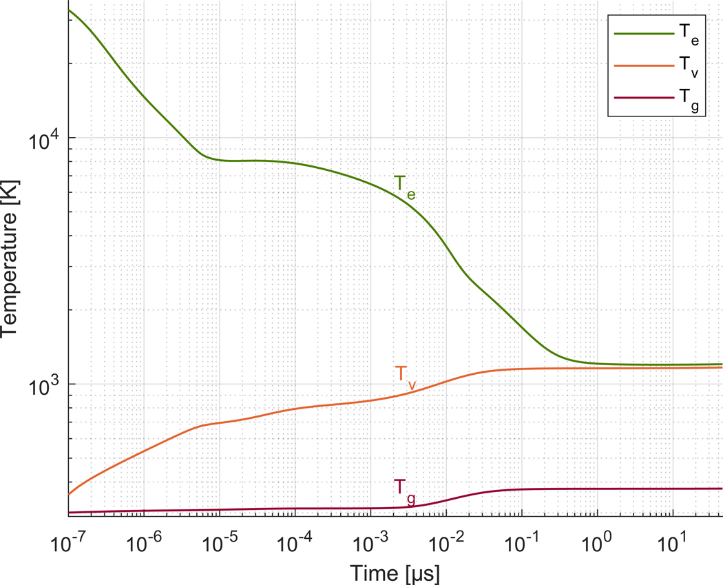
Translational (T_g), vibrational (T_v) and electronic (T_e) temperature in the simulation for nitrogen at 300 K and 101.3 × 10³ Pa. Note T_g(t₀) = T_v(t₀) = 300 K (not shown).

Fast gas heating (described in Section IIC3) provided the bulk of the energy imparted to the translational mode in the model. The absolute rate of translational fast gas heating (Q_tr) monotonically decreased in time (as did heating by elastic collisions, R41) except between $4\times {10}^{-4}\mathrm{\text{μs}}\lesssim t\lesssim 0.05\mathrm{\text{μs}}.$ Over this interval, instead of decreasing, the rate of fast gas heating increased up to 15 fold, causing the inflection in the curve of T_g that began around t ≈ 3 × 10⁻³ μs.

Impact excitation of vibrational modes (R42) primarily drove the growth of T_v until around t ≈ 3 × 10⁻⁴ μs when vibrational fast gas heating (Q_v) overtook it to become the dominant contributor. Similar to fast gas heating for translation, the absolute rate for vibration monotonically decreased in time (as did R42) except over the interval $3\times {10}^{-6}\mathrm{\text{μs}}\lesssim t\lesssim 0.03\mathrm{\text{μs}}$ in which it experienced up to a 22 fold increase, producing the inflection in the curve of T_v that began around t ≈ 3 × 10⁻⁴ μs.

Although fast gas heating dominated the rate contributions for both T_g and T_v at later times, the absolute value of the rate diminished over time by many orders of magnitude. The severely weakened rate could only effect a marginal increase in temperature, explaining the apparent plateau for $t\gtrsim 0.2\mathrm{\text{μs}}\text{.}$

T_e monotonically decreases in time generally much faster than the other temperatures increase. In such a situation, characteristic of a decaying plasma, the electron kinetic energy losses equal or exceed gains. Figure 11 depicts this condition in a set of plots constructed similarly to those previously shown except with absolute rates in units of Ks⁻¹. The figure shows impact dissociation (R40) leading the loss terms at early times, followed by impact excitation of vibrational modes (R42), and then, to a lesser extent, elastic collisions (R41). The (absolute) contribution fraction from R42 remains between about 38–49% after $t\gtrsim 1\times {10}^{-5}\mathrm{\text{μs}}.$ The kinetic energy released by electrons recombining with ions (denoted by dn_e/dt) acts to counter the loss terms. Furthermore, vibrational superelastic collisions (R43) balance the losses at later times, slowing the decay of T_e(t) and causing it to track the value of T_v(t). Three-body electron-ion recombination (R19), which releases U_N⁺, and electronic superelastic collisions (R49) also slow the fall of T_e, but to a much lesser extent.

FIG. 11.

Processes contributing to the rise (solid lines) and fall (dashed lines) of T_e in time with their absolute rates (upper) and contribution fractions (lower). Only processes with a relative contribution of at least 10% are presented.

D. Estimate for Maximum Gas Temperature Rise

An estimate of the maximum rise in translational temperature from complete thermalization of the laser energy imparted during above-threshold ionization is given by

$$\mathrm{\Delta }{T}_{\text{g}}\approx \frac{n_{\text{e}}\left(t_0\right)\left(\frac{3}{2}{k}_{\text{B}}{T}_{\text{e}}\left(t_0\right)+U_{{\text{N}}_2^{+}}\right)}{n_{{\text{N}}_2}(0)c_p}\approx 197\text{K},$$ (34)

with initial conditions from Section IID and nitrogen’s specific heat at constant pressure, $c_p=\frac{7}{2}{k}_{\text{B}}{\text{J K}}^{-1}.$ This value agrees with ΔT_g ≈ 120–230 K found by Edwards et al.⁶ based on fitting a theoretical spectrum (with an elevated rotational temperature) to the observed spectrum of the second positive system. Such an agreement indicates that the model’s values for n_e(t₀) and T_e(t₀) are likely within an order of magnitude of their experimental value. Note that each additional photon of the prototypical above-threshold process increases the temperature rise by roughly 15 K.

E. Initial Electronic Temperature Based on Above Atmospheric Density Experimental Results

Using an image intensifier lens-coupled to a camera, Burns et al.⁸ observed a linear relationship¹⁰⁴ between FLEET initial signal and gas density, $S\left(t_1\right)\propto n_{{\text{N}}_2}(0),$ in nitrogen for $t_1\approx 0.07-0.08\mathrm{\text{μs and}}\frac{n_{{\text{N}}_2}(0)}{n_{\text{STP}}}\approx 1-\mathrm{5.5.}$ For the model to produce a comparable trend over similar densities and time delays, an increased initial electronic temperature (i.e., N_ph,add > 0) was required.

As $n_{{\text{N}}_2}$(0) is increased within the model, the species curves shift earlier in time (due to overall quickening of reactions) and higher in population (due to greater initial densities) relative to the depiction in Figure 5. Additionally, the ‘knees’ of N₂(A), N₂(B) and N₂(C), which occur around t ≈ 0.8–2 μs in Figure 5, shift earlier and higher as well. As T_e(t₀) is increased within the model, the initial growth of N, N₂(A), N₂(B) and N₂(C) prior to 1 × 10⁻⁷ μs is accelerated (due to expedited electron impact reactions) and the dissociation of nitrogen is more complete, yielding a greater ‘steady-state’ concentration of N. The elevated level of N encourages more vigorous atomic recombination, shifting the ‘knees’ in the decay curves of N₂(A), N₂(B) and N₂(C) to earlier times and larger populations. Recall the ability of atomic recombination to enhance not only the lifetime of the B-state, but also the A-state (via quenching of B-state) and the C-state (via energy pooling of A-state). Importantly, when combined with density changes, increasing the initial electronic temperature magnifies the curve shifts (and shifts of the ‘knees’) caused by increased density.

The time and population at which these ‘knees’ occur dictates the signal measured by the gated intensifier. Figure 12 attempts to illustrate this point. If the intensifier’s integration period, Δt_gate, occurs over the steeper part of the curve ahead of the ‘knee,’ any shifting of the curve earlier in time because of density increases will lead to a lower recorded signal (Figure 12, left) and thus an inverse trend. In contrast, when the integration period is taken over the flatter part of the curve after the ‘knee,’ whose value of population increases with density increases, a higher recorded signal results (Figure 12, right). In this way, a higher T_e(t₀) can shift the location of the ‘knee’ to a more favorable time with respect to the integration period (or delay, t₁), causing the recorded signal to increase with increasing density.

FIG. 12.

Increasing density and/or T_e(t₀) shifts the ‘knee’ of the curve in time and magnitude, affecting the recorded signal. For a given t₁ and Δt_gate, at low T_e(t₀), the low density curve will record a greater signal (left), but at high T_e(t₀), the opposite prevails (right).

In the model, T_e(t₀) was set by incrementally increasing the value of N_ph,add in Equation (20) until the signal exhibited an approximately linear relationship with density over the range $\frac{n_{{\text{N}}_2}(0)}{n_{\text{STP}}}\approx 1-5.5$ for a delay t₁ ≈ 0.4 μs and an assumed gate width Δt_gate = 1 μs. Although further increments to N_ph,add enabled the model to better replicate the linear dependence as time delays approached those in the experiment (t₁ ≈ 0.07–0.08 μs), there was concern that the number of additional photons, and thus, the initial electronic temperature, was unrealistically high. Therefore, a compromise of N_ph,add = 2 was used. Measurements of electron temperature (e.g., Thomson scattering) are needed to validate this choice for N_ph,add.

F. Comparison to Below Atmospheric Density Experimental Results

This section compares the model to experimental results at sub-atmospheric conditions. A separate paper¹⁰⁵ will document in greater detail the experimental procedure, data processing approach and additional results.

1. Flow Facility and Intensified Camera Experimental Setup

In a free jet facility custom-built¹⁰⁶ for testing laser-based diagnostics at NASA Langley Research Center, FLEET signal intensities and lifetimes were measured in pure nitrogen (≥ 99.995%) over a range of temperature (72–298K) and pressure (1.7–758Torr) conditions. Gas cylinders supplied high-pressure flow to a converging-diverging nozzle to produce a pressure-matched free jet inside a hermetically sealed and continuously evacuated chamber instrumented for optical access. Regulation of the stagnation pressure controlled the jet’s static pressure. Selection of the nozzle’s expansion contour (subsonic, Mach 1.0, 1.8, 2.7 or 4.0) controlled the jet’s static temperature for near-constant stagnation temperature. For each test condition, schlieren imaging provided confirmation of the absence of shockwaves and collimation of the free jet. High-accuracy sensors tracked the stagnation (plenum), static (chamber wall) and pitot (probe in jet) pressures while a thermocouple monitored the stagnation temperature (plenum).

A fast-framing camera (Photron FASTCAM Mini AX200 CMOS) lens-coupled to a twostage image intensifier (LaVision HighSpeed IRO S25) recorded the FLEET signal using a gate width of Δt_gate = 0.5 μs and time delays of 0.1, 0.2, 0.5, 1, 2, 5, 10.1, 20.1 and 30.1 μs. For early delays, t ≤ 1 μs, the gate width was excessive relative to the decay rate, leading to lifetime measurements longer than actuality (as compared to the PMT results in Figure 4, upper). Maintaining a constant gate width was intended to ensure more consistent comparison across delays (acquired in separate burst series) and avoid introduction of an extra experimental parameter.

A bandpass filter (Semrock custom, 385–771nm) was placed in front of the intensifier’s objective lens (Nikon Nikkor 135mm f/2). Figure 13 shows the filter’s transmission function, T_BP(λ), which passes both the VIS and UV components and thus mixes the two signal contributions. Based on the objective lens’ diameter of D_col = 67.5 × 10⁻³ m and an offset distance from the tagged region of approximately L_col ≈ 0.56m, we estimated a light cone collection efficiency of roughly η_col ≈ 0.09%.

FIG. 13.

Measured spectral transmission function, T_BP(λ), of bandpass filter for image intensifier. Note that filter does not block UV. Taken from Reference 105.

The laser (Spectra-Physics Solstice) was operated at 1000Hz with nominal parameters as before (Section IID2) except for slightly higher pulse energy, U_L ≈ 0.9 × 10⁻³ J, and tighter focusing, f_L = 0.25m. From the model’s perspective, these parameters were essentially equivalent because ionization remained within the tunneling regime (γ_K ≈ 0.24 < 0.5) and the assumption of intensity clamping fixed the laser intensity and thus electron yield. For this focal length, the tagged volume became vol_tag ≈ 2.7 × 10⁻⁶ cm³. The laser beam was oriented radially through the center of the jet to write FLEET lines across its diameter (5.4–10mm) in the core flow.

2. FLEET Image Acquisition and Processing

Over 6600 single-shot measurements were taken at each time delay for every temperature and pressure (density) combination. Each laser shot corresponded to a seven-frame burst of the imaging system. Three frames preceded the laser pulse, clearing the camera sensor of accumulation and ghosting artifacts,¹⁴ and providing a suitable background image for subtraction.¹⁰⁷ Four frames followed the laser pulse, capturing the FLEET signal at the desired delay and additional offsets of 10, 20 and 30 μs. The first six delays (0.1–5 μs) corresponded to independent acquisitions whereas the last three delays (10.1–30.1 μs) came from the same burst as the 0.1 μs delay (i.e., acquired in succession). Therefore, signal analysis relied upon aggregate statistics rather than single-shot values.

The resulting images were dewarped based on a dot card calibration. The tagged line in each image was identified and fit with a series of Gaussian profiles¹⁴ to determine the center and peak signal at each location (i.e., transverse slice) along the FLEET line. Data pruning algorithms filtered out poor fits, outliers or otherwise unacceptable data (e.g., low SNR). Mean and standard deviation statistics were compiled from Gaussian fit results at five central points within the free jet.¹⁰⁸ Results were included in the overall analysis when at least three of the five points exceeded a minimum specified number of single-shot measurements (above 140), otherwise they were excluded. The number of satisfactory single-shot measurements generally started around 6600 at t₁ = 0.1 μs and gradually dwindled with increasing delay up to 2 μs. Beyond 2 μs, or for certain static conditions with short lifetimes, the decrease was more dramatic and fitting Gaussian profiles to the line or even simply distinguishing the signal from noise in the image became problematic.

In an approach similar to the one used to construct Equation (33), we related the signal captured by the intensified camera (at some time delay, t_i) to the rate of change of photon densities within the simulation,

$$\begin{gathered} S_{\text{int}}\left(t_i\right)=({\int }_{t_i}^{t_i+\mathrm{\Delta }{t}_{\text{gnte}}}{r}_{\text{R}3}(t) \\ \times \frac{\int Q{E}_{\text{int}}(\lambda )T_{\text{BP}}(\lambda )r_{\text{ph}}(\lambda ,t)T_{\mathrm{\Delta }{\lambda }_{\text{VIS}}}^{\prime }(\lambda )\text{d}\lambda }{\int r_{\text{ph}}(\lambda ,t)T_{\mathrm{\Delta }{\lambda }_{\text{VIS}}}^{\prime }(\lambda )\text{d}\lambda }\text{d}t \\ +{\int }_{t_i}^{t_i+\mathrm{\Delta }{t}_{\text{gate}}}{r}_{\text{R}4}(t) \\ \times \frac{\int Q{E}_{\text{int}}(\lambda )T_{\text{BP}}(\lambda )r_{\text{ph}}(\lambda ,t)T_{\mathrm{\Delta }{\lambda }_{\text{UV}}}^{\prime }(\lambda )\text{d}\lambda }{\int r_{\text{ph}}(\lambda ,t)T_{\mathrm{\Delta }{\lambda }_{\text{UV}}}^{\prime }(\lambda )\text{d}\lambda }\text{d}t) \\ \times vo{l}_{\mathrm{tag}}{\eta }_{\text{col}}{g}_{\text{int}}, \end{gathered}$$ (35)

where QE_int(λ) was the intensifier’s quantum efficiency given by manufacturer. The tagged volume, vol_tag, and estimated collection efficiency, η_col, were previously calculated for the optical configuration. When using the intensifier with a similar camera (CMOS sensor with 20 μm pixels) and an identical gain setting of 60%, the manufacturer provided the approximate conversion factor of g_int ≈ 35.6 AU.

Similar to before, Equation (32) enables substitution of the Δλ_VIS band of the measured FLEET spectrum (black line in Figure 2) for $r_{\text{ph}}(\lambda ,t)T_{\mathrm{\Delta }{\lambda }_{\text{VIS}}}^{\prime }(\lambda )$ while the UV counterpart to Equation (32) enables substitution of the Δλ_UV band of the spectrum for $r_{\text{ph}}(\lambda ,t)T_{\mathrm{\Delta }{\lambda }_{\text{UV}}}^{\prime }(\lambda ).$

However, unlike before, the resulting equation cannot be solved for photon density rate because of the mixing of the VIS and UV contributions. Therefore, r_R3(t) and r_R4(t) must come from the model and the resulting equation provides a means to compare the model to the experiment in terms of recorded signal (in arbitrary units or AU).

3. Comparison and Analysis of Initial Signal Trends with Density and Temperature

Figure 14 shows the converted modeling (triangles) and experimental (boxes) results for initial signal, S(t₁), with t₁ = 0.1 μs and Δt_gate = 0.5 μs. The experimental markers and error bars correspond to means and standard deviations, respectively, based on approximately 6600 single-shot measurements. The figure illustrates that the initial signal of both the simulation and experiment strongly depends upon density and achieves an optimal value at reduced density, though the optimal point differs between the two curves (0. 11kgm⁻³ and 1.6 × 10⁻² kgm⁻³, respectively). Other experiments^5,100 in nitrogen have similarly shown the maximum (initial) signal occurring at reduced pressure (density) and exceeding the value at atmospheric conditions. Compare the species curves of the atmospheric case¹⁰⁹ in Figure 5 and the near-optimal signal case at similar temperature, but reduced density (0.15kgm⁻³) in Figure 15. The optimization of signal arises not from increased dissociation fraction (see next paragraph), but from retardation of the temporal evolution of the electronically-excited species (due to overall slowing of reactions) which postpones their climax and slows their rate of decay before the opening of the intensifier gate at t = 0.1 μs. Although decreasing the density shifts the population curves later in time, it also depresses their magnitude (due to smaller initial conditions) so that further rarefaction actually reduces the recorded signal. Therefore, for a particular time delay and gate width, there is an optimal value of gas density that maximizes the signal. Recall Section IVE also discusses curve shifts in time and magnitude because of density changes.

FIG. 14.

Simulation (triangles) compared to experiment (boxes) for FLEET initial signal as a function of density and temperature. Simulation accounts for entire tagged region whereas experiment considers only peak signal in center. Error bars correspond to one standard deviation. Taken from Reference 105.

FIG. 15.

Number densities of atoms (solid line), excited molecules (dotted lines) and charged species (dashed lines) in the simulation for nitrogen at 297 K and 13.4 × 10³ Pa. Note that $n_{{\text{N}}_2}(t)\approx 3.2\times {10}^{18}{\text{cm}}^{-3}$ (i.e., 0.15 kg m⁻³).

Dissociation fraction generally increases with decreasing density (as evident in Figure 15) due to a suppression and postponement of the loss pathways for N such as three-body atomic recombination (R1) and certain ion conversion reactions (R29 and R39). Additionally, the low density elongates the timescales of action for impact dissociation (R40) and dissociative recombination (R11 and R12) at early times, while at later times, it prolongs ion conversion such as R32¹¹⁰ and R37, and for the warm cases, three-body electron-ion recombination (R19). Although this situation leads to a larger fraction of atomic nitrogen, it does little to boost the initial signal at low densities because, for the same reasons, atomic recombination proceeds too slowly to affect N₂(B) at the early delays (0.1–0.5us). Furthermore, higher initial gas temperature slightly magnifies the rise in dissociation fraction associated with rarefaction.

Regarding the relative contributions of reactions for N, N₂(A), N₂(B) and N₂(C), decreasing gas density generally elongates the timescales of early reactions (especially lengthening the duration of those involving e^–) and delays the start of later reactions. For N, the later, second peak of the impact dissociation (R40) curve in Figure 6 (lower) subsides. For N₂(B), three-body atomic recombination (R1) becomes less important and fluorescence into B-state (R4) gains some importance at the lowest densities. For N₂(C), energy pooling (R6) and quenching (R26) become relatively less important while fluorescence (R4) grows in importance.

Figure 14 also conveys the weaker influence of gas temperature relative to density in governing initial signal strength. Although colder temperatures consistently produce a stronger signal in the simulation, especially below 0.15kgm⁻³, only the coldest temperatures appear to do so in the experiment. The optimal (peak) signal of the simulation and experiment (at coldest temperature), is merely 30% higher than the corresponding signal at similar density, but warmest temperature. The greatest low temperature signal enhancement takes place at 1.6 × 10⁻² kgm⁻³ for the simulation (a factor of improvement of 3.4 times) and 0.3kgm⁻³ for the experiment (a similar factor of 2.3 times). According to the modeling results, low temperatures favor the formation of cluster ions, boosting the size of the ${\text{N}}_4^{+}$ population. A larger ${\text{N}}_4^{+}$ population accelerates electron-cluster ion dissociative recombination and produces more electronically-excited species (primarily N₂(B) via R8, but also N₂(A) via R7 and N₂(C) via R9). Furthermore, greater B-state population begets greater A- and C-state populations because of the aforementioned coupling mechanisms of energy pooling, quenching and even fluorescence (relatively strengthened by low density). Ultimately, the levels of N₂(A), N₂(B) and N₂(C) are all elevated compared to the warm case, leading to consistently larger recorded signal for delays up to t ≤ 1 μs in the simulation and $t\lesssim 5\mathrm{\text{μs}}$ in the experiment. For this range of conditions, three-body atomic recombination (R1) does not play a vital role in the low temperature enhancement. Retarded by the low densities, R1 rises to prominence far too late (t > 10 μs) to influence the signal at 0.1 μs. Therefore, the magnitude of enhancement suggested by Table II is irrelevant.

In Figure 14, the optimal (0.11 kg m⁻³ and 82 K) and atmospheric reference signals of the simulation exceed the corresponding (i.e., same density and temperature) results of the experiment by 72 and 78 times, respectively. This seemingly great discrepancy in magnitude is partially explained by the fact that the simulation effectively sums the entire signal in the tagged region whereas the experiment only considers the average of the peak signal in the center. In particular, using the apparent thickness of a single pixel (78 × 10⁻⁶ m) instead of the confocal parameter (2.6 × 10⁻³ m) reduces vol_tag and thus the simulation results by roughly 33 times. Furthermore, there is uncertainly in converting the model’s photon density rates into the signal recorded by the intensified camera, namely in vol_tag (which probably changes with conditions), η_col and g_int. Therefore, we regard this factor of agreement acceptable and did not include additional scaling coefficients.

The ratio of optimal signal at reduced density to signal at atmospheric conditions is similar for the simulation (ratio of 9) and experiment (ratio of 18). Unfortunately, the range between the minimum and maximum signal for the simulation disagrees with that of the experiment, exhibiting a total variation of almost two orders of magnitude. A breakdown in the validity of the modeling assumptions may explain this departure from the experimental signal trend at the lowest densities. We relied on a continuum approach to the plasma kinetics (necessary when using rate coefficients from BOLSIG+). However, at the lowest density, the electron mean free path substantially exceeds the beam waist (i.e., radius of the tagged region), ${\lambda }_{\text{MFP},\text{e}}=\sqrt{\frac{8k_{\text{B}}{T}_{\text{e}}}{\pi m_{\text{e}}}}/{\nu }_{\text{elas}}\approx 140\times {10}^{-6}\text{m}⋙{\overline{w}}_0\approx 18\times {10}^{-6}\text{m},$ and a continuum does not accurately represent the rarefied condition. Furthermore, we approximated photoionization as independent of gas density based on the balance between self-focusing and plasma defocusing in Equation (24). However, at very low density, self-focusing weakens relative to geometric focusing and the balance should include the effect of geometric focusing instead of neglecting it. Inclusion of this new term would prevent gas density from simply canceling out, implying a dependence.

V. SUMMARY AND CONCLUSIONS

We proposed a zero-dimensional kinetics model of femtosecond laser ionization in nitrogen with fast gas heating, tuned rate coefficients, electron scattering (elastic and inelastic) from BOLSIG+ and photoionization based on filamentation. The model is summarily described by

$$\begin{array}{c}\text{fs laser}\to n_{{\text{N}}_2^{+}}+n_{\text{e}}+n_{{\text{N}}_2}\to \text{ reactions }\to \\ n_{{\text{N}}_2(\text{B})}+n_{{\text{N}}_2(\text{C})}+\dots \end{array}$$ (36)

At the outset of the simulation, we consider only ${\text{N}}_2^{+}$, e^– and N₂, excluding other species such as atoms (from photodissociation), electronically-excited cations (such as those responsible for first negative emission) or multiply-ionized cations. The plasma and chemical reactions ultimately produce sizable populations of N₂(B) and N₂(C), giving rise to observable visible (to near infrared) and ultraviolet signal, respectively. According to time-resolved measurements using a bandpass-filtered photomultiplier tube (tempered by FLEET spectral measurements), the ultraviolet signal initially dominates until overtaken by the visible signal around t ≈ 2–3 μs. We developed equations to accurately relate the model (which consolidates the emission into two ideal bands) to the experimental measurements (made with a PMT, spectrometer and intensified camera).

At atmospheric conditions, the time-varying signals of the model compare favorably to those from the PMT in terms of absolute magnitude, ratio of VIS to UV and general behavior (fast and slow decay regimes). Regrettably, the model exhibits a noticeably faster decay rate, departing from the experimental results within the first several hundred nanoseconds. This departure limits the applicability of modeling results to the microsecond timescale. We attribute the disagreement to the neglect of fluid dynamics (e.g., gas expansion) and lack of spatial dimensions (e.g., no molecular or ambipolar diffusion) which concentrate all mass into a point and artificially accelerate the reaction rates. Moreover, the energy balance, intended for tracking the swift decay of electronic temperature, only approximately resolves the translational and vibrational temperature evolution. Accurate awareness of translational temperature becomes necessary when considering fluid dynamic effects driven by heating (at the later timescales).

We note that our simplified approach to determining electron scattering rate coefficients neglects the effect of superelastic collisions on the EEDF and the non-equilibrium distribution of vibrational energy. Furthermore, researchers¹¹¹ have shown the importance of considering many vibrational levels (i.e., more than v = 1–8) to better capture both the microscopic (e.g., EEDF, vibrational energy distribution) and macroscopic $(\text{e.g.},{\overline{ϵ}}_{\text{e}},\text{effective}{T}_{\text{v}},n_{\text{N}},n_{{\text{N}}_2}(\text{A}),n_{{\text{N}}_2(\text{B})})$ properties of the plasma. Therefore, an improved version of the model would incorporate a more complete set of cross sections^112,113 for electron impact vibrational excitation and dissociation than the standard dataset accompanying BOLSIG+. Also, accounting for additional vibrational levels would then warrant determining the rates of VT relaxation and dissociation of highly vibrationally excited molecules by atoms.¹¹⁴

The simplicity of the model and its response to changes in rate coefficients affords an opportunity to accurately determine (via tuning) poorly known rate coefficients such as dissociative electron-cluster ion recombination, A- and B-state quenching, and A-state energy pooling. We tune the model to fit the time-resolved PMT measurements at atmospheric conditions, but constrain our tuning to the rate coefficient ranges reported in literature. Given that our effort represents a first attempt at tuning, we emphasize the need for additional refinement and validation of the tuned values.

The electronically-excited states exhibit an interdependence or coupling in time within the model. This coupling arises from the decay cascade of N₂(C) into N₂(B) and then into N₂(A), primarily from collisional quenching, but also from fluorescence (second positive) at the lowest gas densities. Energy pooling by N₂(A) which repopulates N₂(B) and N₂(C) also contributes to the coupling. At long times, these excited species establish a quasi-equilibrium (evident in the figures by their slowed decay) because recombination of N into N₂(B) counteracts the losses sustained by quenching of N₂(A) into N₂. The quasi-equilibrium persists as long as sufficient N population exists.

At atmospheric densities and above, increases to the initial electronic temperature shift the ‘knees’ in the curves (i.e., quasi-equilibrium) of the excited-state populations earlier in time and larger in magnitude. Higher T_e(t₀) yields more complete dissociation of N₂ which naturally accelerates the rate of atomic recombination. More vigorous atomic recombination, combined with the coupling of the excited-state populations, drives the shifts of the ‘knees.’

The model outputs the contribution fraction of the consumption and generation reactions for each of the tracked species (showing figures for the species important to FLEET signal). At atmospheric conditions, electron-containing reactions dominate the earliest timescales (where impact processes lead recombination with ions), followed by quenching, energy pooling and finally, atomic recombination. Changes in initial gas density affect the contribution fractions. In general, decreasing gas density elongates the duration of early reactions and delays the start of later reactions.

Modeling results were compared to intensified camera measurements of FLEET in a variable temperature and pressure free jet. For initial (peak) signal at t₁ = 0.1 μs and Δt_gate = 0.5 μs, the model demonstrated a qualitatively similar trend with initial gas density, achieving an optimal signal at reduced density that exceeded the atmospheric value. Such an optimization holds promise for supersonic and hypersonic measurements that require satisfactory signal at short time delays and gate widths. The optimization arises from shifting the excited species populations in time (delaying their maximum and slowing their decay) such that the intensifier gate captures a higher signal. Since the absolute magnitudes of the population curves decrease with decreasing density, there exists an optimal density for a given time delay and gate width.

Reducing the initial gas temperature slightly enhanced the initial signal for both the simulation and experiment. The increase ranged from 30% to a factor of roughly 2–3. Modeling results indicated the recombination of ${\text{N}}_4^{+}$ cluster ions into excited molecules and their coupling provided the enhancement as opposed to atomic recombination, which occurs too late with respect to the time delay.

At the lowest densities, the model departed from the experiment, experiencing a far greater initial signal roll-off. We attribute this departure to a breakdown in the validity of key modeling assumptions.

Currently, the only comparisons to experiment are based on the first and second positive emissions; however, we desire additional experimental validation of the model. Microwave scattering¹¹⁵ could measure the instantaneous number density of electrons at different initial conditions to validate the photoionization model (probing its gas density dependence) and the overall recombination rate of electrons. Laser Thomson scattering would enable measurement of the initial electronic temperature and its decay in time. Laser absorption (or laser-induced fluorescence) could monitor the population of metastable N₂(A) to justify its size and the rate coefficients of energy pooling (which contribute to the coupling of the excited molecules). We would like to test (or refine) the monolithic assumption for the spectral bands within the time-varying signal. Therefore, we require better spectrally- and time-resolved measurements such as from a photomultiplier with a monochromator to isolate individual rovibrational features (instead of entire bands) and ensure proper extinction of unwanted wavelengths.¹¹⁶ These measurements would initially be taken at atmospheric conditions and then extended to other pressures (and temperatures).

REFERENCES

- 1.In reality, the spectral components of the ‘ultraviolet’ and ‘visible’ signal span the near ultraviolet to blue and yellow to near-infrared, respectively. For brevity, these bands will be referred to simply as ultraviolet and visible throughout the paper.
- 2.McGuire S and Miles R, J. Chem. Phys 141, 244301 (2014). [DOI] [PubMed] [Google Scholar]
- 3.Dogariu A and Miles R, in Air Lasing, Springer Series in Optical Sciences, edited by Polynkin P and Cheng Y (Springer International Publishing, Cham, 2018) Chap. 2, pp. 19–43. [Google Scholar]
- 4.Michael JB, Edwards MR, Dogariu A, and Miles RB, Appl. Opt 50, 5158 (2011). [DOI] [PubMed] [Google Scholar]
- 5.Edwards MR, Femtosecond Laser Electronic Excitation Tagging, B.S.E. thesis, Princeton University, Department of Mechanical & Aerospace Engineering (2012). [Google Scholar]
- 6.Edwards MR, Dogariu A, and Miles RB, AIAA J. 53, 2280 (2015). [Google Scholar]
- 7.Edwards MR, Limbach CM, Miles RB, and Tropina AA, in 53rd AIAA Aerospace Sciences Meeting (AIAA, 2015). [Google Scholar]
- 8.Burns RA, Peters CJ, and Danehy PM, Meas. Sci. Technol 29, 115302 (2018). [DOI] [PMC free article] [PubMed] [Google Scholar]
- 9.Calvert ND, Dogariu A, and Miles RB, in 44th AIAA Plasmadynamics and Lasers Conference (AIAA, 2013). [Google Scholar]
- 10.Dogariu LE, Dogariu A, Miles RB, Smith MS, and Marineau EC, in 2018 AIAA Aerospace Sciences Meeting (AIAA, 2018). [Google Scholar]
- 11.DeLuca NJ, Miles RB, Jiang N, Kulatilaka WD, Patnaik AK, and Gord JR, Appl. Opt 56, 8632 (2017). [DOI] [PubMed] [Google Scholar]
- 12.Miles RB, Edwards MR, Michael JB, Calvert ND, and Dogariu A, in 51st AIAA Aerospace Sciences Meeting Including the New Horizons Forum and Aerospace Exposition (AIAA, 2013). [Google Scholar]
- 13.Peters CJ, Miles RB, Burns RA, Bathel BF, Jones GS, and Danehy PM, in 32nd AIAA Aerodynamic Measurement Technology and Ground Testing Conference (AIAA, 2016). [Google Scholar]
- 14.Peters CJ, Danehy PM, Bathel BF, Jiang N, Calvert ND, and Miles RB, in 31st AIAA Aerodynamic Measurement Technology and Ground Testing Conference (AIAA, 2015). [Google Scholar]
- 15.Burns RA, Danehy PM, and Peters CJ, in 32nd AIAA Aerodynamic Measurement Technology and Ground Testing Conference (AIAA, 2016). [Google Scholar]
- 16.Halls BR, Jiang N, Gord JR, Danehy PM, and Roy S, Appl. Opt 56, E94 (2017). [DOI] [PubMed] [Google Scholar]
- 17.Shneider MN, Baltuka A, and Zheltikov AM, J. Appl. Phys 110, 083112 (2011). [Google Scholar]
- 18.Zhang Y, Calvert N, Shneider MN, and Miles RB, in 32nd AIAA Aerodynamic Measurement Technology and Ground Testing Conference (AIAA, 2016). [Google Scholar]
- 19.For the sake of brevity, implied units such as atoms, molecules, particles, et al. will be omitted here and elsewhere.
- 20.Guerra V, A. S P, and Loureiro J, Eur. Phys. J. Appl. Phys 28, 125 (2004). [Google Scholar]
- 21.Henriques J, Tatarova E, and Ferreira CM, J. Appl. Phys 109, 023301 (2011), rate coefficient for N2(A) + N2 → 2N2 taken from Clark et al. (1980) seems to have been multiplied by 1 × 10². Also, the reaction 2N + N2 → N2(a1Πg) + N2 should actually be a two-body radiative recombination process, i.e., 2N → N2(a1Πg) + h ν, according to the original source Becker et al. (1972). [Google Scholar]
- 22.Popov NA, Plasma Phys. Rep 35, 436 (2009). [Google Scholar]
- 23.Kossyi IA, Kostinsky AY, Matveyev AA, and Silakov VP, Plasma Sources Sci. Technol 1, 207 (1992). [Google Scholar]
- 24.Clyne MAA and Stedman DH, J. Phys. Chem 71, 3071 (1967). [Google Scholar]
- 25.Campbell IM and Thrush BA, Proc. R. Soc. Lond. A 296, 201 (1967). [Google Scholar]
- 26.Becker KH, Fink EH, Groth W, Jud W, and Kley D, Faraday Discuss. Chem. Soc 53, 35 (1972). [Google Scholar]
- 27.Yamashita T, J. Chem. Phys 70, 4248 (1979). [Google Scholar]
- 28.Capitelli M, Ferreira CM, Gordiets BF, and Osipov AI, Plasma Kinetics in Atmospheric Gases, 1st ed., Springer Series on Atomic, Optical, and Plasma Physics (Springer-Verlag Berlin Heidelberg, 2000). [Google Scholar]
- 29.Hays GN and Oskam HJ, J. Chem. Phys 59, 6088 (1973). [Google Scholar]
- 30.Gilmore FR, Laher RR, and Espy PJ, J. Phys. Chem. Ref. Data 21, 1005 (1992). [Google Scholar]
- 31.Lofthus A and Krupenie PH, J. Phys. Chem. Ref. Data 6, 113 (1977). [Google Scholar]
- 32.Hays GN and Oskam HJ, J. Chem. Phys 59, 1507 (1973). [Google Scholar]
- 33.Piper LG, J. Chem. Phys 88, 6911 (1988). [Google Scholar]
- 34.Klopovsky KS, Mukhovatova AV, Popov AM, Popov NA, Popovicheva OB, and Rakhimova TV, J. Phys. D Appl. Phys 27, 1399 (1994). [Google Scholar]
- 35.Popov NA, Phys J D Appl. Phys 44, 285201 (2011). [Google Scholar]
- 36.Gordiets BF, Ferreira CM, Guerra VL, Loureiro JMAH, Nahorny J, Pagnon D, Touzeau M, and Vialle M, IEEE Trans. Plasma Sci 23, 750 (1995), rate coefficient for N2(A) + N2 → 2N2 taken from Clark et al. (1980) seems to have been multiplied by 1 × 10². [Google Scholar]
- 37.Ikezoe Y, Matsuoka S, and Nakamura H, Chem. Phys. Lett 177, 366 (1991). [Google Scholar]
- 38.Keister KE, Wagner CJ, Putney JL, Hewitt JD, and Eden JG, Phys. Rev. A 89, 013401 (2014). [Google Scholar]
- 39.Cao YS and Johnsen R, J. Chem. Phys 95, 7356 (1991). [Google Scholar]
- 40.Popov NA, Plasma Phys. Rep 27, 886 (2001). [Google Scholar]
- 41.Bortner MH and Baurer T, eds., Defense Nuclear Agency Reaction Rate Handbook, 2nd ed. (Department of Defense Nuclear Information & Analysis Center (DASIAC), 1972). [Google Scholar]
- 42.Takaki K, Chang J-S, and Kostov KG, IEEE Trans. Dielectr. Electr. Insul 11, 481 (2004). [Google Scholar]
- 43.Moravej M, Yang X, Barankin M, Penelon J, Babayan SE, and Hicks RF, Plasma Sources Sci. Technol 15, 204 (2006), rate coefficient for taken from Takaki et al. (2004) used wrong unit conversion and should be multiplied by 1.16 × 10⁴. Rate coefficient for e− + N2 → e− + 2N was slightly modified from Park (1988). [Google Scholar]
- 44.Akishev Y, Grushin M, Karalnik V, Petryakov A, and Trushkin N, J. Phys. D Appl. Phys 43, 215202 (2010). [Google Scholar]
- 45.Polak LS, Sergeev PA, and Slovetsky DI, in Plasmachemical Reactions and Processes, edited by Polak LS (Nauka, Moscow, 1977) pp. 87–107. [Google Scholar]
- 46.Slovetsky DI, Mechanisms of Chemical Reactions in Non-Equilibrium Plasmas (Nauka, Moscow, 1980). [Google Scholar]
- 47.Herron JT, J. Phys. Chem. Ref. Data 28, 1453 (1999). [Google Scholar]
- 48.Clark WG and Setser DW, J. Phys. Chem 84, 2225 (1980). [Google Scholar]
- 49.Levron D and Phelps AV, J. Chem. Phys 69, 2260 (1978). [Google Scholar]
- 50.Hunten DM and McElroy MB, Rev. Geophys 4, 303. [Google Scholar]
- 51.Young RA and Saint John GA, J. Chem. Phys 48, 895 (1968). [Google Scholar]
- 52.Thrush BA, J. Chem. Phys 47, 3691 (1967). [Google Scholar]
- 53.Wray KL, J. Chem. Phys 44, 623 (1966). [Google Scholar]
- 54.Piper LG, J. Chem. Phys 97, 270 (1992). [Google Scholar]
- 55.Heidner III RF, Sutton DG, and Suchard SN, Chem. Phys. Lett 37, 243 (1976). [Google Scholar]
- 56.Dreyer JW and Perner D, Chem. Phys. Lett 16, 169 (1972). [Google Scholar]
- 57.Bak MS, Kim W, and Cappelli MA, Appl. Phys. Lett 98, 011502 (2011). [Google Scholar]
- 58.Pereira L, Morozov A, Fraga MM, Heindl T, Krcken R, Wieser J, and Ulrich A, Eur. Phys. J. D 56, 325 (2010). [Google Scholar]
- 59.Hiraoka K and Nakajima G, J. Chem. Phys 88, 7709 (1988), provides equilibrium constant as function of temperature for [Google Scholar]
- 60.Bhringer H and Arnold F, J. Chem. Phys 77, 5534 (1982), provides reverse rate coefficient as function of temperature for [Google Scholar]
- 61.Kaufman F, inChemical Reactions in Electrical Discharges, Advances in Chemistry, Vol. 80, edited by Blaustein BD (American Chemical Society, 1969) Chap. 3, pp. 29–47, assumes rate coefficient for equals that of since molecular velocities are similar. [Google Scholar]
- 62.Dheandhanoo S and Johnsen R, Planet. Space Sci 31, 933 (1983). [Google Scholar]
- 63.Bultel A, Chron BG, and Vervisch P, Plasma Sources Sci. Technol 4, 597 (1995), rate coefficient for e− + N2 → e− + 2N was slightly modified from Park (1988). [Google Scholar]
- 64.Park C, Thermophys J Heat Tr. 2, 8 (1988). [Google Scholar]
- 65.Itikawa Y, J. Phys. Chem. Ref. Data 35, 31 (2006). [Google Scholar]
- 66.Hagelaar GJM and Pitchford LC, Plasma Sources Sci. Technol 14, 722 (2005). [Google Scholar]
- 67.Phelps AV and Pitchford LC, Phys. Rev. A 31, 2932 (1985). [DOI] [PubMed] [Google Scholar]
- 68.LXCat, “SIGLO database,” www.lxcat.net/SIGLO, retrieved on June 4, 2013.
- 69.Blythe AR, Cottrell TL, and Read AW, Trans. Faraday Soc 57, 935 (1961), using the “modified” theory which better agrees with the experimental data. Recall that the rate coefficient, kVT, relates to the relaxation time, γ, via [Google Scholar]
- 70.Cottrell TL and Read AW, J. Chem. Phys 37, 2733 (1962), provides experimental confirmation of the theory of Blythe et al. (1961) for vibrational-translation relaxation in N2 for roughly 500 K to 5500 K. [Google Scholar]
- 71.BOLSIG+’s EEDF is given by (in units of eV−1.5), where F(ϵe) is the EEDF defined in the usual manner.
- 72.The standard installation of BOLSIG+ has cross sections for v = 1–8 and includes both resonant and non-resonant contributions for v = 1.
- 73.McQuarrie DA, Statistical Mechanics, 1st ed. (University Science Books, Mill Valley, California, 2000). [Google Scholar]
- 74.Gorse C and Capitelli M, J. Appl. Phys 62, 4072 (1987). [Google Scholar]
- 75.Capitelli M, Colonna G, De Pascale O, Gorse C, Hassouni K, and Longo S, Plasma Sources Sci. Technol 18, 014014 (2009). [Google Scholar]
- 76.Shneider MN, Zheltikov AM, and Miles RB, Phys. Plasmas 18, 063509 (2011). [Google Scholar]
- 77.Limbach CM and Miles RB, AIAA J. 55, 112 (2017), article describes a higher temperature rise and N2 dissociation fraction in the FLEET tagged region than reported elsewhere (or calculated by the kinetics model). [Google Scholar]
- 78.New-Tolley MR, Shneider MN, and Miles RB, in 2018 Aerodynamic Measurement Technology and Ground Testing Conference (AIAA, 2018) paper uses the elevated temperature rise of Limbach et al. (2017) as input for the simulation to converge with the results of blast wave theory. [Google Scholar]
- 79.We assumed that the much lighter electron third body absorbs all of the energy released during recombination and no energy goes into the translational or vibrational modes of the molecule(s). Furthermore, the dissociation energy of in R10 was neglected.
- 80.DeWitt MJ and Levis RJ, J. Chem. Phys 108, 7739 (1998). [Google Scholar]
- 81.Talebpour A, Yang J, and Chin SL, Opt. Commun 163, 29.(1999), due to a typographical error, the plotted ionization rate of nitrogen should be reduced by a factor of 10 according to Kasparianet al. (2000). [Google Scholar]
- 82.Kasparian J, Sauerbrey R, and Chin SL, Appl. Phys. B 71, 877 (2000). [Google Scholar]
- 83.Couairon A and Mysyrowicz A, Phys. Rep 441, 47 (2007). [Google Scholar]
- 84.Daigle J-F, Jaron-Becker A, Hosseini S, Wang T-J, Kamali Y, Roy G, Becker A, and Chin SL, Phys. Rev. A 82, 023405 (2010). [Google Scholar]
- 85.Bernhardt J, Liu W, Chin SL, and Sauerbrey R, Appl. Phys. B 91, 45 (2008). [Google Scholar]
- 86.Brzsnyi Á, Heiner Z, Kovcs AP, Kalashnikov MP, and Osvay K, Opt. Express 18, 25847 (2010). [DOI] [PubMed] [Google Scholar]
- 87.Zahedpour S, Wahlstrand JK, and Milchberg HM, Opt. Lett 40, 5794 (2015). [DOI] [PubMed] [Google Scholar]
- 88.Wahlstrand JK, Cheng Y-H, and Milchberg HM, Phys. Rev. A 85, 043820 (2012), although measurements were performed at 550–635nm, they also apply to 800nm to within 3%. [DOI] [PubMed] [Google Scholar]
- 89.Xu S, Sun X, Zeng B, Chu W, Zhao J, Liu W, Cheng Y, Xu Z, and Chin SL, Opt. Express 20, 299 (2012). [DOI] [PubMed] [Google Scholar]
- 90.Pressure and density are assumed to be interchangeable in this context.
- 91.An extensive, though certainly non-exhaustive listing of references.
- 92.Stedman DH and Setser DW, J. Chem. Phys 50, 2256 (1969). [Google Scholar]
- 93.Piper LG, J. Chem. Phys 88, 231 (1988). [Google Scholar]
- 94.Valk F, Aints M, Paris P, Plank T, Maksimov J, and Tamm A, J. Phys. D Appl. Phys 43, 385202 (2010). [Google Scholar]
- 95.The pulse energies are effectively equivalent from the point of view of the model.
- 96.We could have alternated between the laser’s first and second harmonic when generating FLEET to produce two separate spectra and then judiciously stitch together a composite spectrum without either laser line. However, we wished to avoid introducing additional experimental parameters into the measurement and therefore used solely 800nm.
- 97.Reaction given by
- 98.Michael JB, Edwards MR, Dogariu A, and Miles RB, in 50th AIAA Aerospace Sciences Meeting Including the New Horizons Forum and Aerospace Exposition (AIAA, 2012). [Google Scholar]
- 99.DeLuca NJ, Femtosecond Laser Electronic Excitation Tagging (FLEET) for a Hypersonic Optical Air Data System, M.S.E. thesis, Princeton University, Department of Mechanical & Aerospace Engineering (2014). [Google Scholar]
- 100.Calvert ND, Femtosecond Laser Electronic Excitation Tagging for Aerodynamic and Thermodynamic Measurements, Ph.D. dissertation, Princeton University, Department of Mechanical & Aerospace Engineering (2016). [Google Scholar]
- 101.The scaling factor required for agreement is reasonable considering the number of estimations and uncertainties required to back calculate the photon density rate in the tagged region.
- 102.When atomic recombination is disabled, the curves for N2(A), N2(B) and N2(C) have no ‘knee’ around t ≈ 0.8–2 μs and instead continue to rapidly decay.
- 103. [With energy pooling disabled, the N2(A) and N2(B) curves look approximately like their counterparts in Figure 5, but the N2(C) curve loses its ‘knee’ around t ≈ 2 μs and instead maintains its rapid descent to eventual zero population.]
- 104.We assume the relationship holds for constant temperature (300 K) and variable pressure.
- 105.Peters CJ, Burns RA, Miles RB, and Danehy PM, “Effect of low temperatures and pressures on signal, lifetime, accuracy and precision of femtosecond laser tagging velocimetry,” (2019), manuscript in preparation. [Google Scholar]
- 106.Designed and assembled by R. A. Burns, C. J. Peters and P. M. Danehy in 2017.
- 107.The camera’s built-in shading (black level) correction made additional background subtraction unnecessary.
- 108.For a given delay, the aggregate mean signal clearly peaked at the center of the jet.
- 109.Although the temperature should match the experiment, the species curves at 300 K are practically indistinguishable from those at 292 K and similar pressure.
- 110.The effect on reaction R32 is especially pronounced for the warm cases.
- 111.Colonna G, Laporta V, Celiberto R, Capitelli M, and Tennyson J, Plasma Sources Sci. Technol 24, 035004 (2015). [Google Scholar]
- 112.Laporta V, Celiberto R, and Wadehra JM, Plasma Sources Sci. Technol 21, 055018 (2012). [Google Scholar]
- 113.Laporta V, Little DA, Celiberto R, and Tennyson J, Plasma Sources Sci. Technol 23, 065002 (2014). [Google Scholar]
- 114.Esposito F, Armenise I, and Capitelli M, Chem. Phys 331, 1 (2006). [Google Scholar]
- 115.Shneider MN and Miles RB, J. Appl. Phys 98, 033301 (2005). [Google Scholar]
- 116.Such an effort would take care to eliminate contamination from second-order diffraction and laser light.