A homogenized constrained mixture (and mechanical analog) model for growth and remodeling of soft tissue

Abstract

Most mathematical models of the growth and remodeling of load-bearing soft tissues are based on one of two major approaches: a kinematic theory that specifies an evolution equation for the stress-free configuration of the tissue as a whole or a constrained mixture theory that specifies rates of mass production and removal of individual constituents within stressed configurations. The former is popular because of its conceptual simplicity, but relies largely on heuristic definitions of growth; the latter is based on biologically motivated micromechanical models, but suffers from higher computational costs due to the need to track all past configurations. In this paper, we present a temporally homogenized constrained mixture model that combines advantages of both classical approaches, namely, a biologically motivated micromechanical foundation, a simple computational implementation, and low computational cost. As illustrative examples, we show that this approach describes well both cell-mediated remodeling of tissue equivalents in vitro and the growth and remodeling of aneurysms in vivo. We also show that this homogenized constrained mixture model suggests an intimate relationship between models of growth and remodeling and viscoelasticity. That is, important aspects of tissue adaptation can be understood in terms of a simple mechanical analog model, a Maxwell fluid (i.e., spring and dashpot in series) in parallel with a “motor element” that represents cell-mediated mechanoregulation of extracellular matrix. This analogy allows a simple implementation of homogenized constrained mixture models within commercially available simulation codes by exploiting available models of viscoelasticity.

1. Introduction

Computational modeling of the growth and remodeling (G&R) of soft tissues has attracted considerable attention over the past two decades. In the mid-1990s, it was suggested that one can capture gross consequences of growth via constitutive equations for the evolution of the stress-free configuration at the tissue level. Importantly, the associated inelastic deformations were incorporated within a multiplicative decomposition of the total deformation gradient into an elastic and inelastic part (Rodriguez, Hoger et al. 1994), not unlike certain models of finite strain plasticity. Because of its conceptual simplicity, this “kinematic growth theory” continues to be used widely (see (Ambrosi, Ateshian et al. 2011, Menzel and Kuhl 2012)), and references therein). Beginning in the late-1990s, however, it was recognized that soft tissue G&R necessarily occurs via mass turnover, including the continuous deposition and degradation of different constituents that form the extracellular matrix (Humphrey and Rajagopal 2002). Again, the associated deformations were considered in terms of a multiplicative decomposition, albeit one that included the deposition of individually prestressed constiutents within the tissue while it is deformed elastically by external loads. This understanding gave rise to a second major class of G&R models based on multi-network theory and known as constrained mixture theories since it was assumed, for simplicity, that the individual constituents deform with the tissue as a whole (see (Ateshian and Humphrey 2012, Valentín and Holzapfel 2012, Cyron and Humphrey 2016) and references therein). Compared with the conceptually simpler kinematic growth models, constrained mixture models are computationally more expensive for they require one to track the history of prior configurations for each of the individually evolving constituents. The advantage of this more complex theory, however, is that cell-mediated mass production and removal can be related more closely with the actual mechanobiology. Indeed, it is because of its closer relationship with the biology that the constrained mixture approach has yielded several important theoretical insights, including that of the driving role of mass turnover in pathologies such as aneurysmal enlargement (Kroon and Holzapfel 2009), the necessity of prestress in living tissue (Cyron and Humphrey 2014), and the concept of mechanobiological stability as a governing principle in physiological and pathological G&R (Cyron and Humphrey 2014, Cyron, Wilson et al. 2014).

In this paper, we seek a computationally less expensive approach that yet preserves some of the salient features of the contrained mixture theory. Specifically, we use an informal temporal averaging to derive a new class of models, which we refer to as homogenized constrained mixture models. This new class of models is shown to agree well with in vitro data for tissue equivalents and to be equivalent to classical constrained mixture models in the linear regime as well as, via one illustrative example, to yield similar results in the nonlinear regime. Unlike classical constrained mixture models, homogenized constrained mixture models do not deal with myriad evolving configurations; rather, they refer to a single time-independent reference configuration and, at each point and for each material species, a time-dependent inelastic local deformation (as in viscoelastic fluids). Interpreted in this way, G&R can be considered as a special type of nonlinear viscoelasticity, represented by a mechanical analog model consisting of a Maxwell fluid in parallel with a motor-element that models cell-mediated mechanoregulation of matrix. In summary, the proposed new class of homogenized constrained mixture models combines the conceptual simplicity and computational efficiency of kinematic growth models (Rodriguez, Hoger et al. 1994) with the well-defined micromechanical foundation of classical constrained mixture models (Humphrey and Rajagopal 2002) and thus provides a promising new approach for multiscale simulations of problems of soft tissue growth and remodeling.

2. Homogenized constrained mixture models

2.1. Basic Kinematics

Let a body with initial (not necessarily stress-free) reference configuration κ(0) be deformed at G&R time s into a current configuration κ(s) so that reference volume elements dV are mapped into current volume elements dv via dv = det(F)dV, where F denotes the usual deformation gradient. Within this standard setting of nonlinear continuum mechanics, we illustrate in Figure 1 both the kinematic growth theory (Rodriguez, Hoger et al. 1994) and the classical constrained mixture model (Humphrey and Rajagopal 2002). In the former, one typically assumes a stress-free reference configuration κ(0). Growth is imagined as a process whereby each infinitesimal volume expands inelastically by the addition of mass. This expansion (which does not stress the volume element) is captured by an inelastic deformation gradient F_g that makes neighboring volume elements in general overlap, that is, it leads to geometrically incompatible configurations. Hence, at each time an additional elastic deformation F_a is required to assemble the individual volume elements elastically into a contiguous body. This elastic deformation combines multiplicatively with a subsequent elastic deformation due to external loads F_E to produce a total elastic deformation F_e = F_EF_a, whereby the total deformation at each G&R time s is

$$F(s)=F_E(s)F_a(s)F_g(s)=F_e(s)F_g(s)$$ (1)

and leads to a configuration of the whole tissue in mechanical equilibrium that satisfies the constraint of geometric compatibility. This kinematic growth theory is conceptually simple but it does not account for the simultaneous presence of different constituents in the body that can have different reference configurations. Moreover, it does not explicity consider mass turnover of individual constituents, including the continuous deposition and degradation that happens in living tissue even in the absence of growth (i.e., changes of tissue mass).

Figure 1:

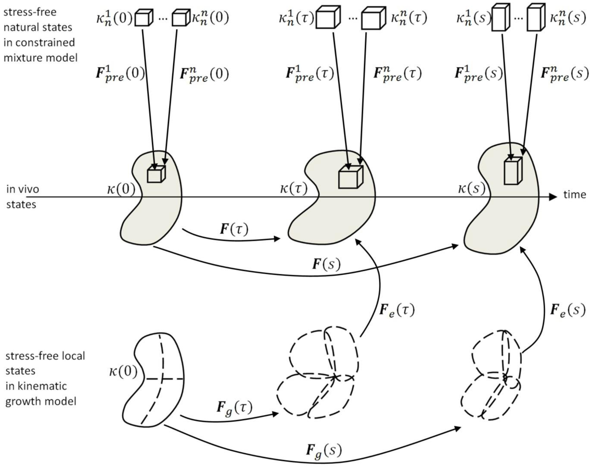
A body in a reference configuration κ(0) is deformed over time into current configurations κ(τ) and κ(t) by external loading and simultaneous growth and remodeling (G&R). In the kinematic growth theory (Rodriguez, Hoger et al. 1994), a stress-free reference configuration κ(0) is assumed, and the total deformation is split into an inelastic growth deformation F_g and an elastic deformation F_e that ensures mechanical equilibrium and geometric compatibility. The inelastic growth deformation F_g alone does not necessarily render a geometrically compatible deformation field but may rather lead to a fictitious intermediate configuration where the body is composed of a (in general infinite) number of patches that may overlap or also form gaps. In contrast, constrained mixture models (Humphrey and Rajagopal 2002) model deformations of individual constituents, with mass added to current configurations at G&R time τ via constituents having a “prestretch” $F_{pre}^{i(\tau )}$ relative to their respective natural (stress-free) configurations ${\kappa }_n^i(\tau )$. Thus, in each volume element there exists simultaneously a mixture of mass increments from n constituents while each constituent itself is a mixture of infinitesimal mass increments deposited during n_t past infinitesimal time intervals (where n_t is infinite in the limit of continuous deformation and G&R). Each of the nn_t mass increments has, in general, a different natural (stress-free) configuration that must be tracked.

To overcome these limitations, constrained mixture models of G&R (Humphrey and Rajagopal 2002) assume that each volume element comprises a constrained mixture of n material constituents (e.g., elastin, families of locally parallel collagen fibers, or smooth muscle) whose respective mechanical quantities are denoted by superscript i ∈ (1, …, n) and which deform together so that different constituents deposited at the same material point X have the same position x¹(X, s) =…= xⁿ(X, s) = x(X, s) ∈ κ(s) in the current configuration. Note, however, that different constituents may exhibit different levels of elastic stretch in κ(s) depending on the portions of their total deformation that are elastic versus inelastic. In this way, constrained mixture models allow different stress-free configurations for different constituents; they can even treat each of the n constituents as consisting of an infinite number of infinitesimal mass increments deposited at each prior time. For example, at G&R time τ ∈ [0, s], infinitesimal mass increments of each of the n constituents can be deposited into the body in configuration κ(τ) with some elastic prestretch $F_{pre}^{i(\tau )}(i=1,\dots ,n)$. Once these increments have been added, they all deform together, with all previously added increments for all constituents, by some F_τ(s) = F(s)F⁻¹(τ) (cf. Figure 1 and Eq. (2) in (Figueroa, Baek et al. 2009)). Thus, at time s the elastic deformation of each mass increment added at time τ is, for the i-th constituent,

$$F_e^{i(\tau )}(s)=F(s)F^{-1}(\tau )F_{pre}^{i(\tau )}.$$ (2)

Importantly, F_τ(s) can be computed regardless of the reference configuration chosen. We can also conceptualize the deformation similar to that in the kinematic growth theory by a decomposition into elastic and inelastic deformation

$$F(s)=F_e^{i(\tau )}(s)F_{gr}^{i(\tau )}(s),$$ (3)

with the inelastic G&R deformation

$$F_{gr}^{i(\tau )}(s)={\left[F_e^{i(\tau )}(s)\right]}^{-1}F(s)={\left[F_{pre}^{i(\tau )}\right]}^{-1}F(\tau ).$$ (4)

That is, the constrained mixture model also enables a multiplicative split into elastic and inelastic deformations, though both quantities generally differ for different mass increments deposited at different times (noting, for example the dependence of $F_e^{i(\tau )}(s)$ on τ via F⁻¹(τ) in (2)) for different constituents. It is for this reason that the classical constrained mixture model (Humphrey and Rajagopal 2002) requires one to track n different natural configurations for the n constituents at each G&R time of deposition τ ∈ [0, s]. In a discrete setting, n_t evaluation times are considered within the time interval [0, s], with n_t ≫ n, and the computational complexity arises mainly from the different references configurations defined at different times.

The motivation for this paper, therefore, is to define an effective, temporally homogenized elastic deformation gradient $F_e^i(s)$ and inelastic deformation gradient $F_{gr}^i(s)$ for each constituent at each G&R time of interest. These homogenized quantities are chosen such that one obtains a similar (and in certain limit cases identical) mechanical behavior for the i-th constituent if one assumes that the whole mass of the i-th constituent exhibits these homogenized elastic and inelastic deformations compared to the case where one thinks of the i-th constituent as composed of a multitude of mass increments deposited at myriad times τ ≤ s, each with a different elastic and inelastic stretch $F_e^{i(\tau )}(s)$ and $F_{gr}^{i(\tau )}(s)$, respectively.

Given any reference configuration κ(0) and external loading on the body, as well as the temporally homogenized inelastic stretch $F_{gr}^i(s)$ up to G&R time s, the homogenized elastic deformation $F_e^i(s)$ can be computed immediately from the condition of mechanical equilibrium and geometric compatibility (cf. (Rodriguez, Hoger et al. 1994)). Thus, given the elastic and inelastic deformations in the initial configuration, all that is required to use homogenized quantities $F_e^i(s)$ and $F_{gr}^i(s)$ is a temporal evolution equation for $F_{gr}^i(s)$. Derivation of this evolution equation is the core of this paper. Note, therefore, that inelastic deformations may result from two processes in a constrained mixture model. First, growth (i.e., a change in mass) leads to an inelastic deformation $F_g^i$ of the reference volume elements in which the mass is deposited or degraded. Second, an additional inelastic deformation $F_r^i$ may result in a constrained mixture simply from the replacement of old mass increments by new mass increments having an, in general, different reference configuration. Such remodeling (i.e., mass exchange) can change the effective traction-free configuration of the i-th constituent without changing its total mass. The total (homogenized) inelastic deformation of the i-th species can thus be written as composition of these two processes, namely

$$F_{gr}^i=F_r^i{F}_g^i.$$ (5)

Thus, the total deformation in a homogenized constrained mixture model is

$$F=F_e^i{F}_{gr}^i=F_e^i{F}_r^i{F}_g^i.$$ (6)

Deriving an evolution equation for $F_{gr}^i$ requires an evolution equation for both the growth $F_g^i$ and the exchange-related remodeling $F_r^i$. The evolution of $F_g^i$ is determined by the amount and orientation of the constituent mass deposited and can thus be defined by standard mechanobiological growth equations (such as the ones used in kinematic or constrained mixture growth models). Thus, only the evolution of the inelastic deformation $F_r^i$ is developed here. Note that the similarity between (1) and (6) implies that homogenized constrained mixture models are as simple to apply as kinematic growth models (Rodriguez, Hoger et al. 1994), while they still rely on the same micromechanical ideas as classical constrained mixture models (Humphrey and Rajagopal 2002).

2.2. Inelastic deformation by mass turnover

We first introduce appropriate quantities to define mass turnover. Let the total current mass of each constituent per volume element dV in the reference configuration κ(0) be called reference mass density ${\varrho }_0^i(s)$; clearly, this quantity changes via mass deposition and degradation. Let ${\dot{\varrho }}_{0+}^i(s)$ be the rate at which constituent mass is deposited per volume dV. As in current constrained mixture models, we assume that each new mass increment ${\dot{\varrho }}_{0+}^i(\tau )d\tau >0$ deposited over the time interval dτ, at time τ, is subsequently degraded such that at time s > τ only the fraction 0 ≤ qⁱ(s, τ) ≤ 1 survives, with qⁱ(s = τ, τ) = 1. Herein we assume mass removal by a Poisson process, that is

$${\dot{q}}^i(s,\tau )=-\frac{1}{T^i}{q}^i(s,\tau )$$ (7)

with some characteristic decay time Tⁱ. Although we could allow inhomogeneous Poisson processes, that is, Tⁱ that vary in time, we restrict these variations to depend on physical state variables that are common for the whole species (e.g., local pH, temperature, or average stress) and do not to depend explicitly on time τ. In the simplest case of a constant Tⁱ, (7) leads to an exponential survival function that is consistent with a first order decay, namely

$$q^i(s,\tau )=\text{exp}\left[-(s-\tau )/T^i\right].$$ (8)

While (7) appears to be a reasonable model in view of known experimental observations, and is key to the homogenization approach developed herein, we emphasize that it necessarily limits the modeling as discussed in Appendix C.

Next, let the rate of mass removal (e.g., degradation) be denoted by ${\dot{\varrho }}_{0-}^i$ whereby from (7) we have

$${\dot{\varrho }}_{0-}^i(s)=-\frac{{\varrho }_0^i(s)}{T^i}.$$ (9)

The total rate of change of reference mass density is thus

$${\dot{\varrho }}_0^i(s)={\dot{\varrho }}_{0+}^i(s)+{\dot{\varrho }}_{0-}^i(s)$$ (10)

which effectively determines the net volume that has to be allocated by $F_g^i$. Hence, all continuum mechanical growth models have to define ${\dot{\varrho }}_0^i(s)$, either directly or indirectly (e.g., via $det\left(F_g^i\right)$). The above model of mass turnover has only one additional free parameter per constituent, the decay time Tⁱ, that is not required in kinematic growth models (Rodriguez, Hoger et al. 1994). This parameter is well-known from constrained mixture models (Humphrey and Rajagopal 2002).

Homogenizing temporally, we seek mechanical parameters and state variables that represent the large number of different mass increments of a constituent deposited over time with, in general, individual natural configurations via a homogeneous material having a single equivalent stress-free configuration and strain energy function. There are various ways to perform such a homogenization, a full review and analysis of which is beyond the scope of this paper. Herein, we pursue a simple temporal homogenization by assuming that mass turnover does not change the general mechanical behavior of a constituent (i.e., its strain energy function), only its average stress-free configuration. To quantify this effect, let new mass of the i-th constituent be deposited with some deposition Cauchy stress ${\sigma }_{pre}^i(s)$. In a constrained mixture of mass increments having the same density (such as the one formed by the myriad mass increments of the i-th constituent deposited over time), the Cauchy stress σⁱ(s) of the mixture becomes the mass-averaged Cauchy stress of all mass increments forming the mixture. Therefore, degrading extant mass with (average) Cauchy stress σⁱ(s) at a rate ${\dot{\varrho }}_{0-}^i(s)$ and depositing new mass with prestress ${\sigma }_{pre}^i(s)$ at a rate ${\dot{\varrho }}_{0+}^i(s)$ induces in a given volume element – if the total deformation F and growth deformation $F_g^i$ are kept constant – in the time interval ds a change in the Cauchy stress

$${\dot{\sigma }}_r^i(s)ds=\frac{{\sigma }_{pre}^i(s){\dot{\varrho }}_{0+}^i(s)ds+{\sigma }^i(s)\left[{\varrho }_0^i(s)+{\dot{\varrho }}_{0-}^i(s)ds\right]}{{\varrho }_0^i(s)+{\dot{\varrho }}_0^i(s)ds}-{\sigma }^i(s)$$ (11)

where the first term on the right-hand side is the mass-averaged Cauchy stress at time s + ds and the second term is the one at time s. Neglecting higher order terms, (11) gives, with (9) and (10),

$${\dot{\sigma }}_r^i(s)=-\frac{{\dot{\varrho }}_{0+}^i\left[{\sigma }^i(s)-{\sigma }_{pre}^i(s)\right]}{{\varrho }_0^i(s)}=-\left[\frac{{\dot{\varrho }}_0^i(s)}{{\varrho }_0^i(s)}+\frac{1}{T^i}\right]\left[{\sigma }^i(s)-{\sigma }_{\mathit{\text{pre}}}^i(s)\right].$$ (12)

The stress rate ${\dot{\sigma }}_r^i(s)$ by mass turnover only (i.e., deposition and degradation of mass increments at a different stress level in a constant geometric configuration) can be expressed, for a given strain energy function, by an equivalent rate of change of the elastic deformation (gradient) ${\dot{F}}_e^i$, that is,

$${\dot{\sigma }}_r^i={\left[\frac{\partial {\sigma }^i}{\partial F_e^i}:{\dot{F}}_e^i\right]}_{F,F_g^i=\mathit{\text{const}}},$$ (13)

while recalling that for (12) we had assumed constant total and growth deformations (i.e., F, $F_g^i=\mathit{\text{const}}$). This assumption leads via its implication $F_e^i{F}_r^i=\mathit{\text{const}}$, with (6), to

$${\dot{F}}_e^i=-F_e^i{\dot{F}}_r^i{\left(F_r^i\right)}^{-1}.$$ (14)

With (14) we can rewrite (13) as

$${\dot{\sigma }}_r^i=-{\left[\frac{\partial {\sigma }^i}{\partial F_e^i}\right]}_{\mathit{F},F_g=\mathit{\text{const}}}:\left[F_e^i{\dot{F}}_r^i{\left(F_r^i\right)}^{-1}\right].$$ (15)

Defining the inelastic remodeling related velocity gradient (cf. Eq. (9) in (Himpel, Kuhl et al. 2005))

$$L_r^i={\dot{F}}_r^i{\left(F_r^i\right)}^{-1},$$ (16)

we arrive (cf. Appendix A) at

$$\left[\frac{{\dot{\varrho }}_0^i(s)}{{\varrho }_0^i(s)}+\frac{1}{T^i}\right]\left[S^i-S_{pre}^i\right]={\left[\frac{\partial S^i}{\partial C_e^i}:\left[C_e^i{L}_r^i+{\left(L_r^i\right)}^T{C}_e^i\right]\right]}_{F,F_g=\mathit{\text{const}}}$$ (17)

with the elastic right Cauchy-Green deformation tensor $C_e^i={\left(F_e^i\right)}^T{F}_e^i$, and the 2^nd Piola-Kirchhoff stresses Sⁱ and prestresses $S_{pre}^i=det(F)F^{-1}{\sigma }_{pre}^i{F}^{-T}$. As pointed out in Appendix A, ${\dot{F}}_r^i$ can be computed in m dimensions from (16) and (17) by solving a system of m(m + 1)/2 linear equations. Then, we can compute with the initial condition $F_r^i=I$ (with identity tensor I) the temporally homogenized inelastic deformation induced by mass turnover at any time. Note that all quantities in (16) and (17) are objective, hence ${\dot{F}}_r^i$ is an objective rate.

2.3. Physical interpretation

The inelastic stress rate by mass turnover described in (12) and (17) can be interpreted in the context of the theory of viscoelastic fluids. To see this, we first introduce the mass-averaged mean prestress of all mass increments forming the i-th species

$${\overline{\sigma }}_{pre}^i(s)={\int }_{-\infty }^s{\sigma }_{pre}^i(\tau )\frac{q^i(s,\tau ){\dot{\varrho }}_{0+}^i(\tau )}{{\varrho }_0^i(s)}d\tau ,$$ (18)

whose time derivative is, with (7),

$$\frac{\partial }{\partial t}{\overline{\sigma }}_{pre}^i(s)={\left[\frac{q^i(s,\tau ){\dot{\varrho }}_{0+}^i(\tau )}{{\varrho }_0^i(s)}{\sigma }_{pre}^i(\tau )\right]}_{s=\tau }-\left[\frac{{\dot{\varrho }}_0^i(s)}{{\varrho }_0^i(s)}+\frac{1}{T^i}\right]{\int }_{-\infty }^{\mathit{t}}\frac{q^i(s,\tau ){\dot{\varrho }}_{0+}^i(\tau )}{{\varrho }_0^i(s)}{\sigma }_{pre}^i(\tau )d\tau .$$ (19)

Using qⁱ(s, s) = 1 and, from (9) and (10), ${\dot{\varrho }}_{0+}^i(s)/{\varrho }_0^i(s)={\dot{\varrho }}_0^i(s)/{\varrho }_0^i(s)+1/T^i$, we can write (19) as

$$\frac{\partial }{\partial t}{\overline{\sigma }}_{pre}^i(s)=\left[\frac{{\dot{\varrho }}_0^i(s)}{{\varrho }_0^i(s)}+\frac{1}{T^i}\right]{\sigma }_{pre}(s)-\left[\frac{{\dot{\varrho }}_0^i(s)}{{\varrho }_0^i(s)}+\frac{1}{T^i}\right]{\overline{\sigma }}_{pre}^i(s).$$ (20)

With this preliminary remark, imagine a body in an initial state with ${\sigma }^i(s)={\sigma }_{pre}^i(s)$ so that turnover does not alter stress over time (cf. (12)). Moreover, assume no change of volume by growth (i.e., ${\dot{F}}_g^i=I$), that is, focus on the effect of mass turnover only, and consider a uniform Heaviside deformation ΔF on the whole body at time $\widehat{s}$. The stress response will be an immediate $\Delta {\sigma }^i={\sigma }^i\left({\widehat{s}}^{+}\right)-{\overline{\sigma }}_{pre}^i$. Subsequently, the system is, by definition, not subject to any further displacement so that evolution of stress is determined by mass turnover alone. The stress rate is thus

$$\frac{\partial }{\partial s}{\sigma }^i(s)={\dot{\sigma }}_r^i(s)=-\left[\frac{{\dot{\varrho }}_0^i(s)}{{\varrho }_0^i(s)}+\frac{1}{T^i}\right]\left[{\sigma }^i(s)-{\sigma }_{pre}^i(s)\right].$$ (21)

Subtracting (20) from (21) gives the stress evolution equation

$$\frac{\partial }{\partial s}\left[{\sigma }^i(s)-{\overline{\sigma }}_{pre}^i\right]=-\left[\frac{{\dot{\varrho }}_0^i(s)}{{\varrho }_0^i(s)}+\frac{1}{T^i}\right]\left[{\sigma }^i(t)-{\overline{\sigma }}_{pre}^i\right],$$ (22)

which implies, for constant prestress, an exponential “active stress recovery” with characteristic time ${\dot{\varrho }}_0^i(s)/{\varrho }_0^i(s)+1/T^i$. This stress recovery can be understood as the stress relaxation of a Maxwell fluid (i.e., a spring and dashpot in series) with a parallel “motor element” (cf. Figure 2), which can thus be considered a mechanical-analog model for materials subjected to mass turnover as considered herein.

Figure 2:

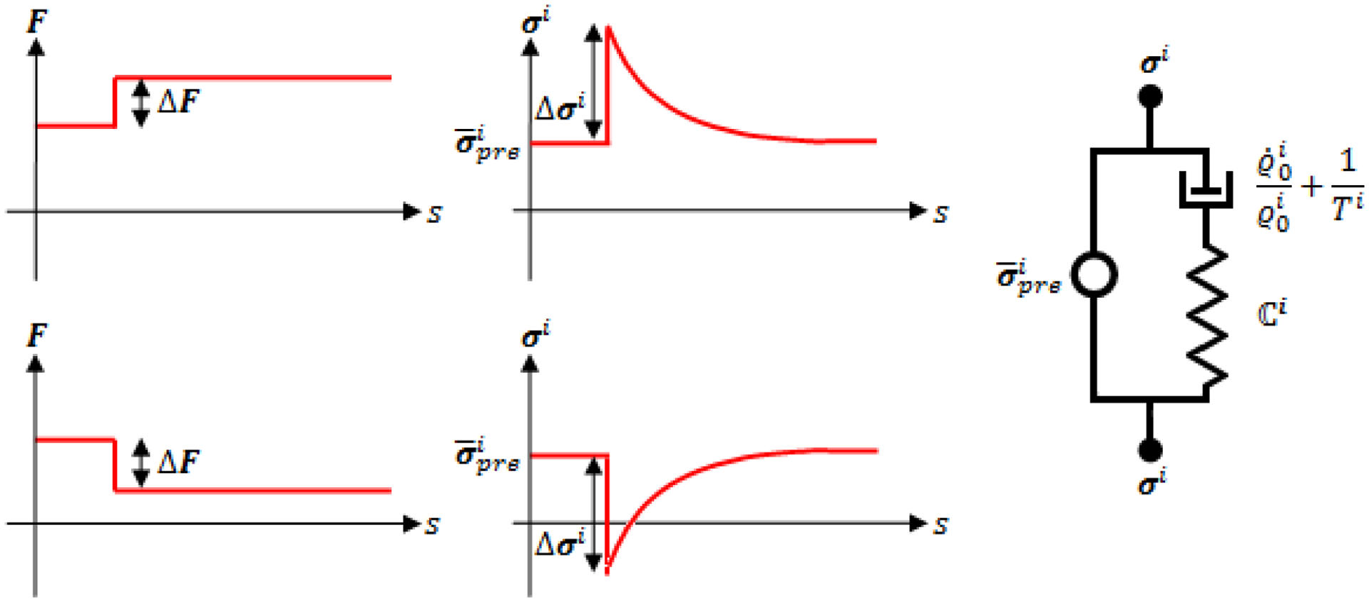
Heaviside perturbation in deformation (left) and resulting instantaneous stress response and “active stress recovery” (center) in a material subject to mass turnover for two different cases: increased deformation or loading (top) and decreased deformation or loading (bottom). Note that stress does not relax towards zero as in typical viscoelastic materials, but instead towards a prestress, which is exactly the behavior of the mechanical analog model on the right: a motor element exerting the stress ${\overline{\sigma }}_{\text{pre}}^i$ in parallel with a Maxwell material (i.e., a dashpot with time constant ${\dot{\varrho }}_0^i(s)/{\varrho }_0^i(s)+1/T^i$ in series with a (in general nonlinear) spring with some stiffness ${ℂ}^i$ that relates deformation increments ΔF and immediate, elastic stress increments Δσⁱ)

In Appendix B we provide an alternative derivation of (22) for the special case of linear elasticity starting from a classical (non-homogenized) constrained mixture model. This derivation demonstrates the close similarity (and equivalence in the linear regime) of the mechanical behavior of classical and temporally homogenized constrained mixture models, and thus the conceptual utility of the mechanical analog model in Figure 2 to both. We also examine in Appendix B the relation between this mechanical analog model and the Volterra equations and kernel functions of the theory of linear viscoelasticity. In Appendix C we discuss mathematical differences between classical and homogenized constrained mixture models for G&R using the idea of “similar sets” introduced in (Rajagopal and Srinivasa 1998). These discussions allow us to review relationships between a “viscoelasticity” induced by mass turnover in living tissue (cf. Figure 2) and classical viscoelasticity of engineering materials.

It is instructive to discuss physical properties of the mechanical analog model in Figure 2. Maxwell bodies are inherently unable to support loads in a static state. The mechanical analog model in Figure 2 can do so only by the motor element in parallel, which models the generation and maintenance of a (average) tissue prestress ${\overline{\sigma }}_{pre}^i(s)$. This confirms the key role of prestress in living tissue suggested in the prestress corollary in (Cyron and Humphrey 2014). The analog model in Figure 2 thus provides an intuitive explanation for the presence of prestress in living tissue – it is a mathematically necessary property of a tissue subject to continuous mass turnover that yet seeks to maintain a static geometry, that is, to establish a so-called mechanobiological equilibrium (Cyron and Humphrey 2014). Extracellular matrix homeostasis thus depends on a cell-mediated mechanoregulation that necessarily includes the incorporation under stress of new constituents within extant matrix (Humphrey, Dufresne et al. 2014).

3. Illustrative examples

3.1. Active stress recovery by remodeling in tissue equivalents

Quantitative validation of mathematical models of G&R is difficult in vivo, but in vitro studies using tissue equivalents can provide the requisite longitudinal mechanical data (e.g., (Bai, Lee et al. 2014)). Indeed, it is sometimes possible to delineate in vitro the separate contributions of growth (changes in mass) and remodeling (changes in microstructure). In this section, we compare the homogenized constrained mixture model developed herein with experimental observations in uniaxial fibroblast-seeded collagen gels (Brown, Prajapati et al. 1998, Ezra, Ellis et al. 2010). Noting the short time scale of these experiments, growth was likely negligible and stress evolution was assumed to be determined solely by load-induced elastic deformations and remodeling according to (12).

Like other cell types, dermal fibroblasts seek to establish a homeostatic level of stress in initially nearly stress-free collagen gels and collagen-GAG sponges (Brown, Prajapati et al. 1998). Perturbation of stress from this homeostatic target induced by a step increase in stretch at time s_P elicits an immediate increase of stress and a subsequent slow recovery of the homeostatic value (see the tension-time data reported in Figure 2a of (Brown, Prajapati et al. 1998)). A host of subsequent papers has examined this phenomenon (see (Simon and Humphrey 2014) for a review) and identified fibroblast-driven remodeling of the collagen network as the underlying mechanism. The elasticity of collagen gels results from different filament-filament interactions mediated by different load-bearing structures within the tissue, such as physical entanglements, secondary bonds, or covalent cross-links. We may imagine remodeling in collagen gels as a continuous degradation of extant load-bearing tissue structures and deposition of new tissue structures representing the remodeled constituents. To capture this turnover with, in general, different half-lives of the different load-bearing tissue structures in fibroblast-driven remodeling, we modeled the gel as a constrained mixture of n collagen fiber families having different decay time constants Tⁱ (cf. (5)). Motivated by the probably nearly constant net heightened stress of the cytoskeleton of the fibroblasts during remodeling, and the assumed intrinsic relation between this stress and the prestress associated with microsructural remodeling, we assumed the same and constant prestress ${\sigma }_{pre}^i(s)={\sigma }_c$ for all fiber families (Note: we use regular instead of bold symbols to emphasize that stresses in this (uniaxial) example are scalars). Recovery of the total Cauchy stress in the gel is thus expected to be the sum of stress relaxations according to (22) for all fiber families, that is, for s > s_P

$$\sigma (s)-{\sigma }_c=\sum _{i=1}^n{\phi }^i\mathit{\text{exp}}\left[-\left(s-s_P\right)/T^i\right]\left[\sigma \left(s_p^{+}\right)-{\sigma }_c\right],$$ (23)

where φⁱ represents the mass fraction of the i-th fiber family, ${\sum }_{i=1}^n{\phi }^i=1$ and $\sigma \left(s_p^{+}\right)$ is the stress immediately after the perturbation at remodeling time s_P. Fitting the experimental data from Figure 2a in (Brown, Prajapati et al. 1998), we found for n = 1 parameters φ¹ = 1.0, T¹ = 11 h with a relative L₂-error of 10% and for n = 2 parameters φ¹ = 0.11, φ² = 0.89, T¹ = 1.0 h, T² = 100 h with a relative L₂-error of 1%, thus suggesting two dominant time scales separated by about two orders of magnitude (cf. Figure 3).

Figure 3:

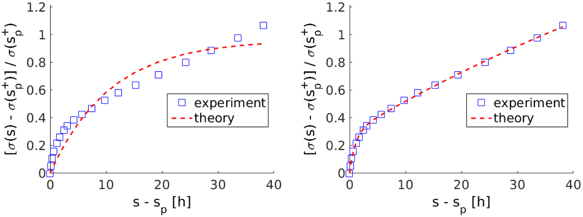
Best fit of (23) to experimental data from Figure 2a in (Brown, Prajapati et al. 1998) for n = 1 (left) and n = 2 (right)

(Ezra, Ellis et al. 2010) compared the recovery of tensional homeostasis in a collagen gel after perturbation for tarsal plate fibroblasts without and with floppy eyelid syndrome. We digitized the experimental data from their Figure 4A separately for each of the perturbations between 8 h and 13.5 h after initiation of the experiment and we normalized the related stress-time curve with respect to the initial deviation from the homeostatic value of stress and the respective perturbation time s_P. Data analysis revealed that the first curve in each and the seventh curve in the floppy eyelid syndrome group were outliers, which were omitted. Analysis of the remaining (superimposed) data revealed that each individual active stress recovery curve could be fit well with a sum of only n = 2 exponentials (with an average relative L₂-error of 1.4%). Fitting the data with n = 2 yielded φ¹ = 0.18, φ² = 0.82, T¹ = 0.05 h, T² = 3.51 h for the 8 curves with floppy eyelid syndrome and φ¹ = 0.41, φ² = 0.59, T¹ = 0.05 h, T² = 1.01 h for the 10 curves without floppy eyelid syndrome (Figure 4).

Figure 4:

Best fit of (23) to experimental data from Figure 4A in (Ezra, Ellis et al. 2010) for n = 1 (left) and n = 2 (right) for tarsal plate fibroblasts without (top) and with (bottom) floppy eyelid syndrome

These results confirm (for data from both (Brown, Prajapati et al. 1998) and (Ezra, Ellis et al. 2010)) that active stress recovery in collagen gels towards a homeostatic value is governed by two dominant time constants. The good agreement between experimental observations in tissue equivalents and our model supports the idea of an intrinsic relationship between remodeling by turnover of mechanical structures and viscoelasticity, which was suggested by the theoretical analysis and model developed herein. An interesting result of our analysis is the presence of two relaxation time constants that differ by about two orders of magnitude in both data sets examined, which suggests two independent remodeling mechanisms in tissue equivalents. Experimental investigation into the physical foundations of these two mechanisms may be a useful avenue of future research. Note, too, that the absolute difference between the time constants observed by (Brown, Prajapati et al. 1998) and (Ezra, Ellis et al. 2010), which is nearly two orders of magnitude, may be understood easily from micromechanical considerations. The remodeling time constant of a specific turnover process is nearly directly proportional to the density (or activity) of driving cellular agents in the material. Therefore, time constants in (Brown, Prajapati et al. 1998) and (Ezra, Ellis et al. 2010) might be understood in the sense that in both systems the same two types of turnover processes dominate, but that cellular density or activity in (Ezra, Ellis et al. 2010) is about two orders of magnitude higher. Finally, the good agreement between our model and experimental data for constant prestress supports this assumption, which has been suggested before (Cyron and Humphrey 2014, Cyron, Wilson et al. 2014).

3.2. Active enlargement of abdominal aortic aneurysms

In this section, we revisit G&R of a model aorta that was examined previously (Cyron, Wilson et al. 2014). Hence, consider an axisymmetric cylindrical membrane whose wall is represented by a constrained mixture of n = 6 constituents: an isotropic elastin matrix, circumferentially oriented smooth muscle, and four collagen fiber families (axial, circumferential, and diagonal at ±45° relative to axial direction). Elastin was modeled as an incompressible neo-Hookean matrix whereas smooth muscle and collagen fibers were modeled as uniaxial (incompressible) fiber families with Fung exponential strain energy functions Ψⁱ. The time constant for mass turnover of collagen and smooth muscle was set to T = 70 d, and growth was governed by

$${\dot{\varrho }}_0^i={\varrho }_0^i(s)k_{\sigma }\frac{{\sigma }^i(s)-{\sigma }_{pre}^i}{{\sigma }_{pre}^i}$$ (24)

where k_σ is a gain-type parameter, and σⁱ and ${\sigma }_{pre}^i$ are the (scalar) Cauchy stress and (constant) prestress in direction of the fiber families. For ease of comparison, all parameter values were identical to the ones used in section 3.4.1 in (Cyron, Wilson et al. 2014). The evolution of stress by growth and remodeling was modeled separately for each species following (17). Because smooth muscle and collagen were modeled as uniaxial fiber families, the associated deformation gradient was given by their rotation and (scalar) stretch ${\lambda }^i={\lambda }_e^i{\lambda }_r^i$, which comprises an elastic stretch ${\lambda }_e^i$ and an inelastic stretch ${\lambda }_r^i$ that arises because of the mass turnover. Thus (17) becomes (cf. Appendix A)

$${\dot{\lambda }}_r^i=\left[\frac{{\dot{\varrho }}_0^i(s)}{{\varrho }_0^i(s)}+\frac{1}{T}\right]\frac{{\lambda }^i}{{\left({\lambda }_e^i\right)}^2}{\left[\frac{\partial {\Psi }^i}{\partial {\lambda }_e^i}+{\lambda }_e^i\frac{{\partial }^2{\Psi }^i}{{\partial }^2{\lambda }_e^i}\right]}^{-1}\left[{\sigma }^i(s)-{\sigma }_{pre}^i\right].$$ (25)

In Figure 5 we compare, for different values of k_σ in (24), results for the classical constrained mixture model (Humphrey and Rajagopal 2002), as implemented in (Cyron, Wilson et al. 2014), directly with those of the temporally homogenized constrained mixture approach introduced herein for the enlargement of an aneurysm following a focal loss of elastin in the central region of the vessel. As expected from the discussion in Appendix B, the results of both approaches are (nearly) identical in the linear regime (i.e., for moderate deformations from the initial state). Perceptible (although still moderate) differences are observed only far away from the linear regime (in our example, only for the two fastest growing aneurysms after ~10 years of simulated time). Recall again that for the classical constrained mixtures models, the reference configurations for each mass increment deposited at each time have to be tracked in the finite element evaluation. We compared in MATLAB the computational cost of the present homogenized constrained mixture approach with the classical one (for which mass increments and their reference configurations were taken into account until degraded by 98%). For a time step size ds = 10 d = T/7, the former surpassed the latter in computational efficiency by around one order of magnitude. This speed-up can be understood from the dominant cost of element evaluation (compared to equation solution) in the problem considered here and the effect of temporal homogenization, which reduces in constrained mixture models the number of operations for element evaluation by around one order of magnitude. As expected, the homogenized constrained mixture model developed herein enabled simulations of G&R at a cost comparable to simulations of standard viscoelastic fluids and well below the one of classical constrained mixture models. The long term differences between the two models remind us, however, that any computational advantage gained via approximations of actual mechanobiological processes must be assessed in individual cases for ultimately we wish to understand the biology, not just minimize computational costs.

Figure 5:

left: axisymmetric model aorta before and 15 years after introducing a focal loss of elastin in the central region shown as a function of the gain parameter k_σ for collagen deposition (note that one can similarly parameterize these simulations in terms of a stability margin m_G&R, which is introduced in (Cyron and Humphrey 2014); right: evolution of the maximal radius R(s) over time s for the same six simulations shown to the left but comparing the classical (dashed lines) and the new homogenized (solid lines) constrained mixture model predictions; note: for m_G&R > 0, the aorta is mechanobiologically stable, that is, the initial defect in elastin does not result in unbounded enlargement of aneurysm, but rather stabilization in a new (typically only slightly dilated) equilibrium (cf. (Cyron and Humphrey 2014, Cyron, Wilson et al. 2014)).

4. Conclusions

There exist computationally efficient models for the G&R of soft tissues that are based on a multiplicative decomposition of the deformation gradient into inelastic (growth-induced) and elastic parts (Rodriguez, Hoger et al. 1994) without explicit incorporation of mass turnover. Nevertheless, actual G&R necessarily results from the turnover of material in potentially evolving configurations and mechanobiologically motivated models should include both mass production and removal (Kroon and Holzapfel 2009, Watton, Selimovic et al. 2011, Wilson, Baek et al. 2013)). Although the models of Watton and colleagues do not, computational models based on classical constrained mixture theory can suffer from high computational costs. In this paper, we proposed a homogenized constrained mixture model that is conceptually as simple and computationally as efficient as the kinematic growth models but incorporates mass turnover on the basis of the idea of a constrained mixture. Using the example of aneurysmal enlargement in a simple model aorta, we demonstrated both the computational efficiency of our new approach and its generally good agreement with the previously developed classical constrained mixture models.

An added advantage of a temporally homogenized constrained mixture approach is that it suggests a simple and intuitive way to understand mechobiologically driven G&R through a mechanical analog model, namely a motor-reinforced viscoelastic Maxwell fluid. The “motor element” represents the actomyosin based cell-mediated creation of a prestress within newly deposited or remodeled matrix, consistent with data that show that cells actively work upon the matrix that they secrete (Humphrey, Dufresne et al. 2014). Given that the form of the classical constrained mixture model was motivated by ideas from multi-network theory and nonlinear viscoelasticity (Humphrey and Rajagopal 2002), a viscoelastic analog model is not surprising. An interesting consequence of such an analog, however, is that soft tissues can maintain a long-term static geometry despite an inherently fluid-like character only because of the deposition prestress, which is in agreement with prior numerical hypothesis testing (Valentin, Cardamone et al. 2009) and a prior study of mechanobiological stability (cf. “prestress corollary” in (Cyron and Humphrey 2014)), which together provide a natural explanation for the apparent omnipresence of prestress in soft tissue.

Another important consequence of our theory relates to the origin of residual stress in soft tissue, which has been hypothesized to originate from geometrically incompatible growth (Rodriguez, Hoger et al. 1994, Vandiver and Goriely 2009). Our analysis suggests that residual stresses introduced by incompatible growth could – at least in tissues with pronounced mass turnover such as arteries – quickly relax due to the fluid-like character of soft tissue G&R and that residual stresses are therefore likely to originate rather from deposition prestresses than incompatible growth. This interpretation is supported by the experimental observation that residual stress forms in vitro in initially relaxed collagen gels as soon as fibroblasts begin to remodel the matrix in an attempt to establish a homeostatic state of stress (Simon and Humphrey 2014, Simon, Murtada et al. 2014), although no macroscopically incompatible growth processes occur in these gels since there is no frank mass addition. Note, too, that in capturing experimental observations on remodeling in tissue equivalents (Brown, Prajapati et al. 1998, Ezra, Ellis et al. 2010), our model suggests further that G&R may well be driven by not one, but rather two or more, structural turnover processes (recall the two characteristic time constants associated with Figure 3 and Figure 4 above). Identification and examination of the precise micromechanical mechanisms corresponding to these distinct turnover processes should be a promising avenue of future research.

In summary, although we focused on G&R in soft tissue, the general derivation of our model from a classical constrained mixture theory suggests potential broader applicability of the viscoelasticity-based mechanical analog model, including potential utility in studying creep-like deformations in bone (as observed, e.g., in orthodonics (Hannon and Knapp 2006)), G&R-related behaviors of biofilms (Albero, Ehret et al. 2014), and likely many other cases. Clearly, much remains to be explored in the general area of the biomechanics of growth and remodeling and its myriad applications.

Appendix A

In general, (cf. Eqs. (6.10) and (6.11) in (Holzapfel 2000))

$$\frac{\partial {\sigma }^i}{\partial F_e^i}:{\dot{F}}_e^i=\frac{\partial {\sigma }^i}{\partial C_e^i}:{\dot{C}}_e^i=\frac{\partial {\sigma }^i}{\partial C_e^i}:\left[{\left({\dot{F}}_e^i\right)}^T{F}_e^i+{\left(F_e^i\right)}^T{\dot{F}}_e^i\right].$$ (A1)

With (A1), (14), (15), and the (symmetric) elastic Cauchy-Green deformation tensor $C_e^i={\left(F_e^i\right)}^T{F}_e^i$, we can rewrite (13) as

$${\dot{\sigma }}_r^i=-{\left[\frac{\partial {\sigma }^i}{\partial C_e^i}:\left[C_e^i{L}_r^i+{\left(L_r^i\right)}^T{C}_e^i\right]\right]}_{F,F_g=\mathit{\text{const}}}$$ (A2)

or equivalently with (12) as

$$\left[\frac{{\dot{\varrho }}_0^i(s)}{{\varrho }_0^i(s)}+\frac{1}{T^i}\right]\left[{\sigma }^i-{\sigma }_{pre}^i\right]={\left[\frac{\partial {\sigma }^i}{\partial C_e^i}:\left[C_e^i{L}_r^i+{\left(L_r^i\right)}^T{C}_e^i\right]\right]}_{F,F_g=\mathit{\text{const}}}.$$ (A3)

Using (cf. Eq. (6.12) in (Holzapfel 2000))

$${\sigma }^i=\frac{1}{J}F{S}^i{F}^T,$$ (A4)

with Sⁱ the 2^nd Piola-Kirchhoff stresses and J = det(F) the Jacobi determinant, plus the condition F, F_g = const, we rewrite (A3) as

$$\frac{1}{J}\left[\frac{{\dot{\varrho }}_0^i(s)}{{\varrho }_0^i(s)}+\frac{1}{T^i}\right]F\left[S^i-S_{pre}^i\right]F^T={\left[\frac{1}{J}F\frac{\partial S^i}{\partial C_e^i}:\left[C_e^i{L}_r^i+{\left(L_r^i\right)}^{\mathit{T}}{C}_e^i\right]F^{\mathit{T}}\right]}_{F,F_g=\mathit{\text{const}}}$$ (A5)

or

$$\left[\frac{{\dot{\varrho }}_0^i(s)}{{\varrho }_0^i(s)}+\frac{1}{T^i}\right]\left[S^i-S_{pre}^i\right]={\left[\frac{\partial S^i}{\partial C_e^i}:\left[C_e^i{L}_r^i+{\left(L_r^i\right)}^T{C}_e^i\right]\right]}_{F,F_g=\mathit{\text{const}}}.$$ (A6)

Noting the symmetries of Sⁱ, $S_{pre}^i$, and $C_e^i$, (A6) provides in m dimensions (if $\partial S^i/\partial C_e^i$ has full rank) m(m + 1)/2 equations to determine the six unknowns of the symmetric part of $C_e^i{L}_r^i$, leaving the skew symmetric part undefined. Similar problems are well-known from (anisotropic) plasticity and are often addressed by additional micromechanically motivated kinematic or constitutive conditions (Dafalias 1998), including the simple assumption that the undetermined skew symmetric part is zero. A general discussion of this issue is beyond the scope of this paper. It is worth mentioning, however, that both for isotropic materials and for quasi-one-dimensional fiber families, it is sufficient to decompose $F_r^i=R_r^i{U}_r^i$ into a rotation tensor $R_r^i$ and a (symmetric) stretch tensor $U_r^i$ (as common in nonlinear continuum mechanics) and to assume $R_r^i=I$ (with identity tensor I). Then $C_e^i{L}_r^i=C_e^i{\dot{U}}_r^i{\left(U_r^i\right)}^{-1}$ so that (A6) becomes a system of m(m + 1)/2 ordinary differential equations in time that enables computation of the m(m + 1)/2 components of $U_r^i$. For isotropic materials the assumption $R_r^i=I$ is justified by the rotation invariance of the strain energy function. For quasi-one-dimensional fiber families it results from the micromechanical modeling assumption that during mass turnover new fibers are deposited always in the same direction (in reference configuration).

In case of a rank deficient stiffness $\partial S^i/\partial C_e^i$, there are deformation modes in $F_r^i$ that do not contribute to strain energy and that can (and have to) be chosen arbitrarily. For example, for (incompressible) quasi-one-dimensional fiber families aligned in direction A_i in the by $F_g^i$ deformed intermediate configuration (and thus also in the by $F_{gr}^i=F_r^i{F}_g^i$ deformed second intermediate configuration due to the assumption $R_r^i=I$ for such fibers), we can choose

$$F_r^i={\lambda }_r^i{A}_i\otimes A_i+\frac{1}{\sqrt{{\lambda }_r^i}}\left(I-A_i\otimes A_i\right),$$ (A7)

where only the inelastic stretch ${\lambda }_r^i$ in fiber direction is unknown and all other deformation modes (except for the volumetric one) are arbitrarily chosen such as to ensure zero inelastic shear deformation. Then the general equation

$${\sigma }^{\mathit{i}}=\frac{1}{J}\frac{\partial {\Psi }^{\text{i}}\left(F_e^i\right)}{\partial F}{F}^T=\frac{1}{J}\frac{\partial {\Psi }^{\text{i}}}{\partial F_e^i}\frac{\partial F_e^{\mathit{i}}}{\partial F}{F}^T=\frac{1}{J}\frac{\partial {\Psi }^{\text{i}}}{\partial F_e^i}{\left(F_{gr}^i\right)}^{-1}{F}^T=\frac{1}{J}\frac{\partial {\Psi }^{\text{i}}}{\partial F_e^i}{F}_e^i,$$ (A8)

simplifies in the fiber direction due to the unit Jacobi determinant J = 1 to

$${\sigma }^{\mathit{i}}=\frac{\partial {\Psi }^{\text{i}}}{\partial {\lambda }_e^i}{\lambda }_e^i,$$ (A9)

and thus

$${\left[\frac{\partial {\sigma }^{\mathit{i}}}{\partial {\lambda }_e^i}\right]}_{F,F_g^i=\mathit{\text{const}}}^{-1}={\left(\frac{\partial {\Psi }^{\text{i}}}{\partial {\lambda }_e^i}+\frac{{\partial }^2{\Psi }^i}{{\partial }^2{\lambda }_e^i}{\lambda }_e^i\right)}^{-1}.$$ (A10)

with elastic and inelastic fiber stretches ${\lambda }_e^i$ and ${\lambda }_r^i$ and Cauchy stress σⁱ in fiber direction. Then (A3) yields with $\partial {\lambda }_e^i/\partial {\left({\lambda }_e^i\right)}^2=1/\left(2{\lambda }_e^i\right)$ the scalar evolution equation

$${\dot{\lambda }}_r^i=\left[\frac{{\dot{\varrho }}_0^i(s)}{{\varrho }_0^i(s)}+\frac{1}{T^i}\right]\frac{{\lambda }^i}{{\left({\lambda }_e^i\right)}^2}{\left[\frac{\partial {\Psi }^i}{\partial {\lambda }_e^i}+{\lambda }_e^i\frac{{\partial }^2{\Psi }^i}{{\partial }^2{\lambda }_e^i}\right]}^{-1}\left[{\sigma }^i-{\sigma }_{pre}^i\right],$$ (A11)

which allows to compute the only unknown component of $F_r^i$ in (A7).

Appendix B

In this appendix we examine, assuming a classical non-homogenized constrained mixture model, in the linear regime the relation between mass turnover and the theory of viscoelasticity. In this theory, stress is generally expressed by the Volterra equation

$${\sigma }^i(s)={\int }_{-\infty }^s{G}^i(s-\tau ):\dot{\epsilon }(\tau )d\tau$$ (A12)

where the kernel function Gⁱ is a fourth order tensor, ε is the (linear) engineering strain tensor, and the colon denotes a double contraction product. The Cauchy stress for a mass increment produced at time τ′ equals in the linear elastic regime its prestress plus the stress from the deformation ε(s) − ε(τ′) that the mass increment experienced between its deposition at time τ′ and the current time s, that is,

$${\sigma }^i(s)={\sigma }_{pre}^i\left(\tau \prime \right)+{ℂ}^{\mathit{i}}:\left[\epsilon (s)-\epsilon \left(\tau \prime \right)\right]={\sigma }_{pre}^i\left(\tau \prime \right)+{ℂ}^i:{\int }_{-\infty }^{s}h\left(\tau -\tau \prime \right)\dot{\epsilon }(\tau )d\tau$$ (A13)

where ${ℂ}^i$ is the fourth order elasticity tensor and h(τ − τ′) is the Heaviside step function. The i-th constituent in each volume element comprises, in general, mass increments produced in the time interval]−∞; s]. At time s, the mass fraction of an increment produced in the time interval dτ′ at τ′ is $q^i\left(s,\tau \prime \right){\dot{\varrho }}_{0+}^i\left(\tau \prime \right)d\tau \prime /{\varrho }_0^i(s)$ so that, according to the classical constrained mixture approach (Humphrey and Rajagopal 2002), the (mass-averaged) Cauchy stress of the i-th species is, with (18),

$$\begin{gathered} {\sigma }^i(s)={\overline{\sigma }}_{pre}^i(s)+{ℂ}^{\mathit{i}}:{\int }_{-\infty }^s{\int }_{-\infty }^{s}h\left(\tau -\tau \prime \right)\dot{\epsilon }(\tau )d\tau \frac{q^i\left(s,\tau \prime \right){\dot{\varrho }}_{0+}^i\left(\tau \prime \right)}{{\varrho }_0^i(s)}d\tau \prime = \\ ={\overline{\sigma }}_{pre}^i(s)+{ℂ}^{\mathit{i}}:{\int }_{-\infty }^s{\int }_{-\infty }^{s}h\left(\tau -\tau \prime \right)\frac{q^i\left(s,\tau \prime \right){\dot{\varrho }}_{0+}^i\left(\tau \prime \right)}{{\varrho }_0^i(s)}d\tau \prime \dot{\epsilon }(\tau )d\tau = \\ {\overline{\sigma }}_{pre}^i(s)+{\int }_{-\infty }^s\underset{G^i(s-\tau )}{\underbrace{{\int }_{-\infty }^s\frac{q^i\left(s,\tau \prime \right){\dot{\varrho }}_{0+}^i\left(\tau \prime \right)}{{\varrho }_0^i(s)}d\tau \prime {ℂ}^{\mathit{i}}}}:\dot{\mathit{\epsilon }}(\tau )d\tau ={\overline{\sigma }}_{pre}^i(s)+{\int }_{-\infty }^s{G}^{\mathit{i}}(s-\tau ):\dot{\epsilon }(\tau )d\tau \end{gathered}$$ (A14)

Given the physiological requirement qⁱ(s → ∞, τ′) = 0, we conclude from (A12) and (A14) that mass turnover makes a body behave like a viscoelastic fluid with the special kernel function

$$G^i(s-\tau )={\int }_{-\infty }^{\tau }\frac{q^i\left(s,\tau \prime \right){\dot{\varrho }}_{0+}^i\left(\tau \prime \right)}{{\varrho }_0^i(s)}d\tau \prime {ℂ}^{\mathit{i}}.$$ (A15)

Note that, by definition, the current density ${\varrho }_0^i(s)$ equals the sum of the surviving fractions qⁱ(s, τ′) of all mass increments ${\dot{\varrho }}_{0+}^i\left(\tau \prime \right)d\tau \prime$ previously deposited per unit volume, that is,

$${\varrho }_0^i(s)={\int }_{-\infty }^s{q}^i\left(s,\tau \prime \right){\dot{\varrho }}_{0+}^i\left(\tau \prime \right)d\tau \prime$$ (A16)

and therefore $G^i(0)={G^i(s-\tau )|}_{\tau =s}={ℂ}^i$.

To understand the mechanical implications of (A14), we consider its time derivative (after subtracting ${\overline{\sigma }}_{pre}^i(s)$)

$$\frac{\partial }{\partial s}\left({\sigma }^i(s)-{\overline{\sigma }}_{pre}^i(s)\right)={\left[G^{\mathit{i}}(s-\tau ):\dot{\epsilon }(\tau )\right]}_{\tau =s}+{\int }_{-\infty }^s\frac{\partial }{\partial s}{G}^{\mathit{i}}(s-\tau ):\dot{\epsilon }(\tau )d\tau .$$ (A17)

The time derivative of (A15)

$$\frac{\partial }{\partial s}{G}^{\mathit{i}}(s-\tau )=-\frac{{\dot{\varrho }}_0^i(s)}{{\varrho }_0^i(s)}\frac{{ℂ}^{\mathit{i}}}{{\varrho }_0^i(s)}{\int }_{-\infty }^{\tau }{q}^i\left(s,\tau \prime \right){\dot{\varrho }}_{0+}^i\left(\tau \prime \right)d\tau \prime +\frac{{ℂ}^{\mathit{i}}}{{\varrho }_0^i(s)}{\int }_{-\infty }^{\tau }\frac{\partial }{\partial s}{q}^i\left(s,\tau \prime \right){\dot{\varrho }}_{0+}^i\left(\tau \prime \right)d\tau \prime ,$$ (A18)

with (7), gives

$$\frac{\partial }{\partial s}{G}^{\mathit{i}}(s-\tau )=-\left[\frac{{\dot{\varrho }}_0^i(s)}{{\varrho }_0^i(s)}+\frac{1}{T^i}\right]G^{\mathit{i}}(s-\tau ),$$ (A19)

which leads, with (A17) and $G^i(0)={ℂ}^i$, to

$$\frac{\partial }{\partial s}\left({\sigma }^i(s)-{\overline{\sigma }}_{pre}^i(s)\right)={ℂ}^{\mathit{i}}:\dot{\epsilon }(s)-\left[\frac{{\dot{\varrho }}_0^i(s)}{{\varrho }_0^i(s)}+\frac{1}{T^i}\right]{\int }_{-\infty }^s{G}^{\mathit{i}}(s-\tau ):\dot{\epsilon }(\tau )d\tau$$ (A20)

and, with (A14), finally to

$$\frac{\partial }{\partial s}\left({\sigma }^i(s)-{\overline{\sigma }}_{pre}^i(s)\right)={ℂ}^{\mathit{i}}:\dot{\epsilon }(s)-\left[\frac{{\dot{\varrho }}_0^i(s)}{{\varrho }_0^i(s)}+\frac{1}{T^i}\right]\left[{\sigma }^i(s)-{\overline{\sigma }}_{pre}^i(s)\right],$$ (A21)

This stress evolution equation is equivalent to (22), recalling that in (22) we had considered a Heaviside deformation step, that is, $\dot{\epsilon }(s>\widehat{s})=0$. Therefore, in the linear limit the classical constrained mixture approach based on multi-network theory, as introduced by (Humphrey and Rajagopal 2002), is equivalent to the homogenized constrained mixture approach developed herein, which explains the similar results of both in Figure 5 and supports the appropriateness of our homogenization scheme. We conclude that the mechanical analog model in Figure 2 is therefore also appropriate for understanding the general behavior of classical constrained mixture models. Conversely, the kernel function in (A15) is also applicable to the homogenized constrained mixture model (noting the unique relation between kernel function and stress evolution).

Appendix C

It is instructive to compare the mathematical and physical basis of classical and homogenized constrained mixture models for G&R. Mathematically, classical models are based on multi-network theory and assume that the total strain energy of the constrained mixture equals the sum of the strain energy of all mass increments, and that the strain energy functions Ψⁱ(τ, F) of mass increments of the i-th constituent deposited at time τ form for all τ a “similar set” in the sense of Definition 3 in (Rajagopal and Srinivasa 1998) (and remain constant in time s). This means, for any τ and $\widehat{\tau }$ there exist $F_{gr}^{i(\tau )}$ and $F_{gr}^{i(\widehat{\tau })}$ such that for any F

$${\Psi }^i\left(\tau ,F{\left(F_{gr}^{i(\tau )}\right)}^{-1}\right)={\Psi }^i\left(\widehat{\tau },F{\left(F_{gr}^{i(\widehat{\tau })}\right)}^{-1}\right)$$ (26)

In other words, the strain energy function of different mass increments of the same constituent differs only by some inelastic deformation. By contrast, in homogenized constrained mixture models we assume that the strain energy function Ψⁱ(s, F) of the whole constituent (which may change in time) belongs at any two times s and $\widehat{s}$ to the same “similar set”, that is, for any F there exist $F_{gr}^i(s)$ and $F_{gr}^i(\widehat{s})$ such that

$$\Psi \left(s,F{\left(F_{gr}^i(s)\right)}^{-1}\right)=\Psi \left(\widehat{s},F{\left(F_{gr}^i(\widehat{s})\right)}^{-1}\right)$$ (27)

This difference in the mathematical basis has a nice interpretation in the context of soft matter physics. Nonlinear constitutive behaviors of polymeric materials can result from different mechanisms. For example, they may result from the nonlinear stiffness of the single fibers, which are immersed in a thermal bath and behave like nonlinear entropic springs (cf. Eq. (6.14) in (Howard 2001) or Eq. (8.10) in (Mofrad and Kamm 2006) or (Cyron and Wall 2009, Cyron and Wall 2012)). Let in such a setting a certain group of the fibers persist while another group is degraded and replaced by new fibers in a different nonlinear stretch state. The elastic behavior of the resulting mixture cannot, in general, be described by averaging the nonlinear strain of both groups of fibers (e.g., on the basis of their respective mass fractions) because of the non-linearity of the stress-response of each group of fibers. Rather, one has to keep track separately of the nonlinear strain states of both groups and average only their strain energy or Cauchy stress on the basis of mass fractions. In a first approximation, one may neglect thereby interactions between different fiber groups (e.g., by cross-linking molecules), which are not assumed to contribute significantly to the nonlinear behavior of the material. This idea is formalized in multi-network theory, which was developed to understand inelasticity of remodeling rubber materials (Rajagopal and Wineman 1992) whose nonlinear behavior largely depends on the nonlinear entropic elasticity of single fibers (Mark, Erman et al. 2013) as discussed above.

In other polymeric materials, however, nonlinear elasticity mainly results from reorientation of fibers in the network (Onck, Koeman et al. 2005, Stein, Vader et al. 2011) during deformation. Again, let a certain group of fibers in such networks persist while another group is degraded and replaced by new fibers with a different stress-free configuration. The mechanical nonlinearity of the resulting mixture crucially depends on the orientation distribution of the fibers. This orientation distribution can be approximated by the average orientation of both fiber groups, which motivates models based on one average elastic strain for the whole mixture such as homogenized constrained mixture models. At the same time, in this setting (cross-linker-mediated or steric) interactions between subgroups of fibers often play an important role, which complicates application of multi-network theory (and thus classical constrained mixture models) where such interactions are generally neglected.

Both classical and the homogenized constrained mixture models rely on assumptions that will in general form only approximations of the actual complex micromechanical behavior of a soft tissue. It is interesting to note, however, that the origin of the mechanical nonlinearity of collagen gels has been assumed to lie rather in fiber reorientation during large deformation (Stein, Vader et al. 2011) than, for example, in entropic elasticity of single fibers, which physically motivates application of homogenized constrained mixture models to G&R of soft tissue. It is, however, worth mentioning that homogenized constrained mixture models suffer, despite their otherwise favorable properties, from a potential drawback compared to the classical ones (Humphrey and Rajagopal 2002). Since the latter keep track of all single mass increments produced at any time in the network, they allow arbitrary survival functions qⁱ(s, τ). Any approach involving homogenization across all mass increments of the i-th constituent, such as the one developed herein, can necessarily allow only dependences of qⁱ(s, τ) on quantities common for all mass increments of the species, which excludes for example a specific dependence on the deposition time τ (and thus explicit age) of an individual mass increment. Potential limitations associated with (7) should thus be kept in mind and it may be an interesting avenue of future research to examine better the structural basis for the the assumptions made in (7) based on specific experiments.

Homogenized constrained mixture models are based on a multiplicative decomposition of the deformation gradient into an elastic and inelastic part and thus in certain aspects similar to classical approaches to plasticity or viscoelastic fluids (Reese and Govindjee 1998). Nevertheless, there are some important differences. The first and perhaps most important one is prestress: stress evolution in our approach depends crucially on some prestress ${\sigma }_{pre}^i(s)$, represented in Figure 2 by a motor element in parallel to the Maxwell body. This element is missing in common models of viscoelasticity or plasticity where inelastic deformation is driven by relaxation of some overstress rather than via active intervention by microscopic agents (cells) that seek to enforce some non-zero stress level (like collagen producing cells in G&R). A second important difference of homogenized constrained mixture models to classical nonlinear viscoelasticity (Reese and Govindjee 1998, Simo and Hughes 2000) as well as recent G&R models (Himpel, Kuhl et al. 2005, Ambrosi, Ateshian et al. 2011, Menzel and Kuhl 2012) is the law of stress evolution which in our case is not motivated in any way by the Clausius-Duhem inequality, but rather is derived from assumptions on the micromechanical foundations of G&R. This way we avoid the problem of the undefined extra-entropy term complicating the derivation of a stress evolution law (Himpel, Kuhl et al. 2005). Clearly, more work is needed to derive a thermomechanical basis for G&R.

References

- Albero AB, Ehret AE and Böl M (2014). “A new approach to the simulation of microbial biofilms by a theory of fluid-like pressure-restricted finite growth.” Computer Methods in Applied Mechanics and Engineering 272: 271–289. [Google Scholar]
- Ambrosi D, Ateshian GA, Arruda EM, Cowin SC, Dumais J, Goriely A, Holzapfel GA, Humphrey JD, Kemkemer R, Kuhl E, Olberding JE, Taber LA and Garikipati K (2011). “Perspectives on biological growth and remodeling.” J Mech Phys Solids 59(4): 863–883. [DOI] [PMC free article] [PubMed] [Google Scholar]
- Ateshian GA and Humphrey JD (2012). “Continuum models of biological growth and remodeling: past successes and future opportunities.” Annu Rev Biomed Engr 14: 97–111. [DOI] [PubMed] [Google Scholar]
- Bai Y, Lee PF, Humphrey JD and Yeh AT (2014). “Sequential multimodal microscopic imaging and biaxial mechanical testing of living multicomponent tissue constructs.” Ann Biomed Eng 42(9): 1791–1805. [DOI] [PMC free article] [PubMed] [Google Scholar]
- Brown RA, Prajapati R, McGrouther DA, Yannas IV and Eastwood M (1998). “Tensional homeostasis in dermal fibroblasts: mechanical responses to mechanical loading in three-dimensional substrates.” J Cell Physiol 175(3): 323–332. [DOI] [PubMed] [Google Scholar]
- Cyron C and Wall W (2012). “Numerical method for the simulation of the Brownian dynamics of rod-like microstructures with three-dimensional nonlinear beam elements.” International Journal for Numerical Methods in Engineering 90(8): 955–987. [Google Scholar]
- Cyron CJ and Humphrey JD (2014). “Vascular homeostasis and the concept of mechanobiological stability.” International Journal of Engineering Science 85(0): 203–223. [DOI] [PMC free article] [PubMed] [Google Scholar]
- Cyron CJ and Humphrey JD (2016). “Growth and remodeling of load-bearing soft tissues.” Meccanica submitted. [DOI] [PMC free article] [PubMed] [Google Scholar]
- Cyron CJ and Wall WA (2009). “Finite-element approach to Brownian dynamics of polymers.” Physical Review E 80(6): 066704. [DOI] [PubMed] [Google Scholar]
- Cyron CJ, Wilson JS and Humphrey JD (2014). “Mechanobiological stability: a new paradigm to understand the enlargement of aneurysms?” Journal of The Royal Society Interface 11(100). [DOI] [PMC free article] [PubMed] [Google Scholar]
- Dafalias YF (1998). “Plastic spin: necessity or redundancy?” International Journal of Plasticity 14(9): 909–931. [Google Scholar]
- Ezra DG, Ellis JS, Beaconsfield M, Collin R and Bailly M (2010). “Changes in fibroblast mechanostat set point and mechanosensitivity: an adaptive response to mechanical stress in floppy eyelid syndrome.” Invest Ophthalmol Vis Sci 51(8): 3853–3863. [DOI] [PMC free article] [PubMed] [Google Scholar]
- Figueroa CA, Baek S, Taylor CA and Humphrey JD (2009). “A Computational Framework for Fluid-Solid-Growth Modeling in Cardiovascular Simulations.” Comput Methods Appl Mech Eng 198(45–46): 3583–3602. [DOI] [PMC free article] [PubMed] [Google Scholar]
- Hannon P and Knapp K (2006). Forensic Biomechanics, Lawyers & Judges Publishing Company. [Google Scholar]
- Himpel G, Kuhl E, Menzel A and Steinmann P (2005). “Computational modelling of isotropic multiplicative growth.”
- Holzapfel G (2000). Nonlinear Solid Mechanics: A Continuum Approach for Engineering, John Wiley & Sons Ltd. [Google Scholar]
- Howard J (2001). Mechanics of Motor Proteins and the Cytoskeleton, Sinauer Associates, Publishers. [Google Scholar]
- Humphrey JD, Dufresne ER and Schwartz MA (2014). “Mechanotransduction and extracellular matrix homeostasis.” Nat Rev Mol Cell Biol 15(12): 802–812. [DOI] [PMC free article] [PubMed] [Google Scholar]
- Humphrey JD and Rajagopal KR (2002). “A constrained mixture model for growth and remodeling of soft tissues.” Mathematical Models and Methods in Applied Sciences 12(03): 407–430. [Google Scholar]
- Kroon M and Holzapfel GA (2009). “A theoretical model for fibroblast-controlled growth of saccular cerebral aneurysms.” J Theor Biol 257(1): 73–83. [DOI] [PubMed] [Google Scholar]
- Mark JE, Erman B and Roland M (2013). The Science and Technology of Rubber, Elsevier Science. [Google Scholar]
- Menzel A and Kuhl E (2012). “Frontiers in growth and remodeling.” Mechanics Research Communications 42(0): 1–14. [DOI] [PMC free article] [PubMed] [Google Scholar]
- Mofrad MRK and Kamm RD (2006). Cytoskeletal Mechanics: Models and Measurements in Cell Mechanics, Cambridge University Press. [Google Scholar]
- Onck P, Koeman T, Van Dillen T and Van der Giessen E (2005). “Alternative explanation of stiffening in cross-linked semiflexible networks.” Physical review letters 95(17): 178102. [DOI] [PubMed] [Google Scholar]
- Rajagopal K and Srinivasa A (1998). “Mechanics of the inelastic behavior of materials—Part 1, theoretical underpinnings.” International Journal of Plasticity 14(10): 945–967. [Google Scholar]
- Rajagopal KR and Wineman AS (1992). “A constitutive equation for nonlinear solids which undergo deformation induced microstructural changes.” International Journal of Plasticity 8(4): 385–395. [Google Scholar]
- Reese S and Govindjee S (1998). “A theory of finite viscoelasticity and numerical aspects.” International journal of solids and structures 35(26): 3455–3482. [Google Scholar]
- Rodriguez EK, Hoger A and McCulloch AD (1994). “Stress-dependent finite growth in soft elastic tissues.” J Biomech 27(4): 455–467. [DOI] [PubMed] [Google Scholar]
- Simo JC and Hughes TJR (2000). Computational Inelasticity, Springer; New York. [Google Scholar]
- Simon DD and Humphrey JD (2014). Learning from Tissue Equivalents: Biomechanics and Mechanobiology. Bio-inspired Materials for Biomedical Engineering, John Wiley & Sons, Inc.: 281–308. [Google Scholar]
- Simon DD, Murtada SI and Humphrey JD (2014). “Computational model of matrix remodeling and entrenchment in the free-floating fibroblast-populated collagen lattice.” International Journal for Numerical Methods in Biomedical Engineering 30(12): 1506–1529. [DOI] [PubMed] [Google Scholar]
- Stein AM, Vader DA, Weitz DA and Sander LM (2011). “The micromechanics of three-dimensional collagen-I gels.” Complexity 16(4): 22–28. [Google Scholar]
- Valentin A, Cardamone L, Baek S and Humphrey JD (2009). “Complementary vasoactivity and matrix remodelling in arterial adaptations to altered flow and pressure.” J R Soc Interface 6(32): 293–306. [DOI] [PMC free article] [PubMed] [Google Scholar]
- Valentín A and Holzapfel GA (2012). “Constrained mixture models as tools for testing competing hypotheses in arterial biomechanics: a brief survey.” Mech Res Comm 42: 126–133. [DOI] [PMC free article] [PubMed] [Google Scholar]
- Vandiver R and Goriely A (2009). “Morpho-elastodynamics: The long-time dynamics of elastic growth.” Journal of biological dynamics 3(2–3): 180–195. [DOI] [PubMed] [Google Scholar]
- Watton PN, Selimovic A, Raberger NB, Huang P, Holzapfel GA and Ventikos Y (2011). “Modelling evolution and the evolving mechanical environment of saccular cerebral aneurysms.” Biomech Model Mechanobiol 10(1): 109–132. [DOI] [PubMed] [Google Scholar]
- Wilson JS, Baek S and Humphrey JD (2013). “Parametric study of effects of collagen turnover on the natural history of abdominal aortic aneurysms.” Proc. R. Soc. A 469(2150): 20120556. [DOI] [PMC free article] [PubMed] [Google Scholar]