Annotating cell types in human single-cell RNA-seq data with CellO

Summary

Cell type annotation is important in the analysis of single-cell RNA-seq data. CellO is a machine-learning-based tool for annotating cells using the Cell Ontology, a rich hierarchy of known cell types. We provide a protocol for using the CellO Python package to annotate human cells. We demonstrate how to use CellO in conjunction with Scanpy, a Python library for performing single-cell analysis, annotate a lung tissue data set, interpret its hierarchically structured cell type annotations, and create publication-ready figures.

For complete details on the use and execution of this protocol, please refer to Bernstein et al. (2021).

Graphical abstract

Highlights

• •CellO is a Python package for annotating cell types in single-cell RNA-seq data
• •CellO classifies cells against the hierarchically structured Cell Ontology
• •CellO can be integrated into single-cell analysis pipelines implemented with Scanpy
• •We present a tutorial that classifies cells in an existing lung tumor data set

Cell type annotation is important in the analysis of single-cell RNA-seq data. CellO is a machine-learning-based tool for annotating cells using the Cell Ontology, a rich hierarchy of known cell types. We provide a protocol for using the CellO Python package to annotate human cells. We demonstrate how to use CellO in conjunction with Scanpy, a Python library for performing single-cell analysis, annotate a lung tissue data set, interpret its hierarchically structured cell type annotations, and create publication-ready figures.

Before you begin

Cell type annotation is an important task in the analysis of single-cell RNA-seq data. CellO (Bernstein et al., 2021) is a machine learning-based tool for annotating cells using the Cell Ontology (Bard et al., 2005). The Cell Ontology is a knowledgebase of known cell types structured as a directed acyclic graph (DAG) in which nodes in the graph represent cell types and edges represent “is a” relationships between cell types. By annotating cells using cell types from the Cell Ontology, CellO’s outputs are hierarchical. That is, if a cell is labeled as a given cell type, it is also labeled as all ancestors of that cell type according to the DAG. Framing the cell type annotation task as that of hierarchical classification has the advantage that if the algorithm is unsure about annotating a cell as a specific cell type (e.g., CD4+ T cell), it can label the cell using a more general term (e.g., T cell). Thus, CellO is capable of providing informative cell type labels for cells that may be difficult to annotate. Lastly, CellO is trained on a collection of purified bulk RNA-seq datasets from diverse cell types and thus, CellO can classify both bulk and single-cell RNA-seq data. When classifying single-cell RNA-seq data, CellO classifies cell clusters.

The protocol below describes the steps required for annotating cell types in a lung tissue sample produced by Laughney et al. (2020) via the 10× Genomics Chromium platform, a platform for performing droplet-based single-cell RNA-seq. Specifically, we will annotate cells in sample GSM3516673 in the Gene Expression Omnibus (GEO; Edgar et al., 2002). CellO accepts as input a variety of file types that may store the input gene expression matrix including comma-separated value (CSV), tab-separated value (TSV), HDF5, as well as the collection of files that are produced by the 10× Genomics Chromium data processing pipeline. The data set that we will use in this protocol (from Laughney et al.) will be downloaded as a CSV file.

CellO can be executed in two ways: either using a set of command line functions in a terminal window or within Python. CellO’s command line functions are intended for users who may not have extensive experience working with Python. Instructions for using CellO’s command line tools can be found in the README.md file in CellO’s GitHub repository (https://github.com/deweylab/CellO).

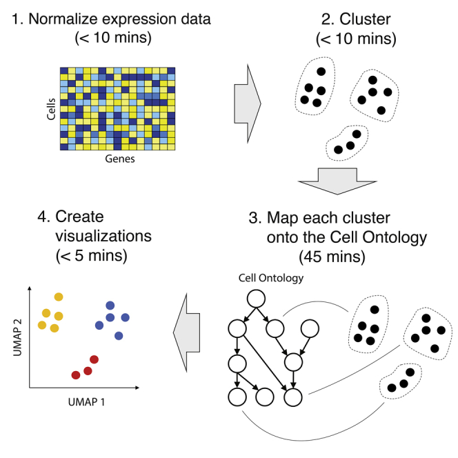
In this protocol, we will describe how to run CellO within Python using CellO’s Python API (Figure 1). This protocol’s target audience are users who are familiar with Python and wish to integrate CellO into their Python-based single-cell analysis pipelines. CellO’s API follows the conventions employed by the Scanpy Python package (Wolf et al., 2018) for performing general single-cell analyses and thus, CellO can easily be integrated into an existing RNA-seq analysis pipeline implemented with Scanpy. All steps in this tutorial are implemented within a Jupyter notebook. This notebook is available in CellO’s GitHub repository and can also be executed in a web browser via Google Colab. A link to the Colab notebook can be found in the GitHub repository’s README.md file (https://github.com/deweylab/CellO/blob/master/README.md).

Figure 1.

Schematic overview

A schematic overview of the steps required to run this protocol.

Prepare your gene expression matrix

Timing: 2 min

• 1.
  Prepare your gene expression matrix as a comma-separated value (CSV) file.

  • a.
    In this tutorial, we will use sample GSM3516673 from GEO, which is a lung tissue sample produced by Laughney et al. (2020). This file can be downloaded from the command line with the following command:

    • curl -O
    • ftp://ftp.ncbi.nlm.nih.gov/geo/samples/GSM3516nnn/GSM35166 73/suppl/GSM3516673_MSK_LX682_NORMAL_dense.csv.gz

CRITICAL: The input CSV file must have the cells ids stored in the first column and the gene ids stored in the first row.

CRITICAL: CellO requires that the genes are represented as either gene symbols or Entrez gene IDs. When possible, we suggest using Entrez gene IDs in order to minimize ambiguity. When provided with gene symbols, CellO will attempt to map these symbols to Entrez gene IDs and will ignore genes for which the Entrez ID is unknown.

Key resources table

REAGENT or RESOURCE	SOURCE	IDENTIFIER
Deposited data
Lung tissue single-cell RNA-seq data set	Laughney et al. (2020)	GEO: GSM3516673
Software and algorithms
CellO v2.0.2	Bernstein et al., 2021	https://github.com/deweylab/CellO
Jupyter Notebook implementing this protocol for CellO v2.0.2	This study	https://github.com/deweylab/CellO/blob/master/tutorial/cello_tutorial.ipynb
Scanpy	Wolf et al., 2018	https://scanpy.readthedocs.io
leiden-alg	Traag et al., 2019	https://github.com/vtraag/leidenalg
Anaconda	Anaconda Inc.	https://anaconda.org
PyGraphviz		https://pygraphviz.github.io/documentation/stable/index.html#

Step-by-step method details

Install the CellO package and its dependencies using Anaconda

Timing: 10 min

• 1.
  Install CellO and its dependencies

  • a.
    Create an isolated virtual environment using Anaconda. To do so, run the following commands in your terminal window, hitting enter after each line:

    • conda activate
    • conda create -y -n cello_env python=3.7 graphviz
    • conda activate cello_env
  • b.
    At the command line within the terminal window, run the following commands:

    • pip install pygraphviz leidenalg scanpy cello-classify
  • c.
    If you wish to implement this protocol using the provided Jupyter notebook, then you will need to install Jupyter as well. To do so, run the following command:

    • pip install jupyter

• 2.
  Verify that CellO is installed correctly

  • a.
    At the command line within the terminal window, run the command:

    • python
      This will start the Python shell. Once running, run the following command:
    • import cello
      Once finished, you can exit the Python shell by typing Ctrl+D.

• 3.
  Optional: Download and launch the Jupyter notebook that implements this protocol

  • a.
    Download the CellO tutorial Jupyter notebook from GitHub. To do so, at the command line, enter the following command:

    • curl -O
      https://raw.githubusercontent.com/deweylab/CellO/master/tutorial/cello_tutorial.ipynb
  • b.
    Launch the Jupyter notebook. To do so, run the following command:

    • jupyter notebook cello_tutorial.ipynb
  • c.
    After entering this command, the Jupyter notebook will open automatically in your computer’s default web browser.

Load the expression matrix into Python and preprocess the data

Timing: 5 min

• 4.
  Import necessary Python packages

  • a.
    Run the following commands in the Python shell to import the Python packages that we will need for this protocol:

    • import cello
    • import os
    • import pandas as pd
    • import scanpy as sc
    • from anndata import AnnData

• 5.
  Load the single-cell expression matrix using Pandas and Scanpy

  • a.
    We will load the expression matrix into a Pandas dataframe. From this dataframe, we will instantiate an AnnData object. AnnData objects represent annotated single-cell expression matrices and are used by the Scanpy library. To perform these steps, run the following Python commands:

    • df = pd.read_csv(
    •  "GSM3516673_MSK_LX682_NORMAL_dense.csv.gz",
    •  index_col=0
      )
    • adata = AnnData(df)

      Note: AnnData objects use the rows of the data matrix to store the observations (i.e., cells) and the columns to store the features (i.e., genes). Thus, in this protocol, the expression matrix is a cell-by-gene matrix rather than a gene-by-cell matrix.

• 6.
  Normalize and cluster the data

  • a.
    Variant 1: Normalize and cluster the data explicitly using Scanpy.

    • i.
      Normalize expression data into units of log transcripts per million (TPM). This can be accomplished with the following calls to Scanpy:
      sc.pp.normalize_total(adata, target_sum=1e6)
      sc.pp.log1p(adata)
    • ii.
      Annotate the 10,000 most highly expressed genes for performing clustering. Note, that CellO will operate on all of the genes. These most highly expressed genes will be used only for clustering and visualization.
      sc.pp.highly_variable_genes(adata, n_top_genes=10000)
    • iii.
      Perform principal component analysis (PCA). To cluster the data in Scanpy, we first compute the first 50 principal components of each sample using PCA. This can be performed with Scanpy using the following command:
      sc.pp.pca(
      adata,
      n_comps=50,
      use_highly_variable=True
      )
    • iv.
      Compute nearest-neighbors graph. Before we run Leiden, we must compute the nearest neighbors graph on the cells. We do so by finding the nearest 15 cells to each cell using the Euclidean distance between the first 50 principal components. This can be performed with Scanpy using the following command:
      sc.pp.neighbors(adata, n_neighbors=15)
    • v.
      Cluster the cells with Leiden. This can be performed with Scanpy using the following command:
      sc.tl.leiden(adata, resolution=2.0)
  • b.
    Variant 2: Using CellO’s wrapper function. CellO provides a wrapper function for normalizing and clustering a UMI counts matrix provided as an AnnData object by wrapping the steps in Variant 1 above:
    cello.normalize_and_cluster(
     adata,
     n_pca_components=50,
     n_neighbors=15,
     n_top_genes=10000,
     cluster_res=2.0
    )

    CRITICAL: CellO requires that the input expression matrix is normalized using estimated transcripts per million (TPM) and then transformed via log(TPM+1). For UMI count data, TPM are equivalent to counts per million (CPM). CellO’s normalize_and_cluster wrapper function performs this normalization for UMI data specifically. For non-UMI count data, the steps required to derive log(TPM+1) will depend on the units of expression. For a discussion on TPM and its relationships to other units of expression, such as reads per kilobase per million mapped reads (RPKM), see Li et al. (2010).

    CRITICAL: CellO must operate on dense expression profiles resembling those produced by bulk RNA-seq assays. To run CellO on single-cell data, we cluster the single cells and aggregate the sparse expression profiles of the cells within each cluster to form a dense expression profile. Furthermore, because CellO operates on cell clusters, it is important that the cells are not under-clustered. The Leiden algorithm’s resolution parameter controls the granularity of clusters. To increase cluster granularity, the resolution parameter should be increased. In this protocol, we use a resolution of 2.0, which is higher than the default value provided by Scanpy. We set this parameter higher in order to avoid under-clustering. On new data, we encourage the user to examine the quality of the clusters via dimension-reduction scatterplots, such as UMAP plots (see Step 11), in order to detect under clustering.

  • 7.
    Optional: Use pre-computed, custom clusters

    • a.
      If one has loaded, or computed, a Python list storing each cell’s cluster assignment, where the i^th element of the list is the cluster id corresponding to the i^th cell’s cluster, then one can store these clusters within the AnnData object, adata, in order to be annotated by CellO. For example, if this Python list is called ‘clusts’, then one can run the Python statement:
      adata.obs['clusters'] = clusts

This statement will create a new column in the adata.obs dataframe called “clusters” with the content of the clusts list.

CRITICAL: The list, clusts, must store cluster ids for cells that are ordered in the same order as the rows of adata.obs.

Classify cells with CellO

Timing: 45 min

• 8.
  Specify CellO’s resource location

  • a.
    We specify the location of CellO’s resources database. CellO requires a database storing pre-trained models as well as training data for training new models. These data are stored in a directory named “resources”. If this directory is not present in the target location, CellO will download it automatically and store it at the target location. We specify this location as follows:

    • cello_resource_loc = os.getcwd()

  CRITICAL: CellO’s resources database requires approximately 5GB of disk space.

• 9.
  Run CellO

  • a.
    Variant 1: Training a new model. CellO will examine the input gene expression matrix and determine whether the genes match those expected by one of CellO’s pre-trained models. If the genes expected by the pre-trained models are not a subset of the genes in the provided expression matrix, CellO will train a new model using CellO’s built-in training set. This model can be saved and re-used for classifying future datasets that assay the expression of these same genes.

    • i.
      Specify the file prefix for CellO’s newly trained model. The file storing the model will be named <prefix>.model.dill:

      • model_prefix = 'GSM3516673_MSK_LX682_NORMAL′
    • ii.
      Run CellO using the following command:

      • cello.scanpy_cello(
      •  adata,
      •  clust_key='leiden',
      •  rsrc_loc=cello_resource_loc,
      •  out_prefix=model_prefix,
      •  log_dir=os.getcwd()
      • )
        If not found, CellO will download the resources and place them in cello_resource_loc. Also, if using custom clustering, the clust_key parameter should be set to the name of the column in adata.obs that stores each cell’s cluster.

        Note: CellO is packaged with pre-trained models that were trained using CellO’s built-in training set. Each pre-trained model was trained using a different subset of genes. CellO will check whether the input expression matrix is comprised of expression data for the same set of genes as those on which a pre-trained model was trained. If no matching model can be found, then a new model will need to be trained using the built-in training set on the subset of genes shared by the training set and the given gene expression matrix. In Step 9.a above, we train a new model according to the genes in the current gene expression matrix. During training, CellO will output a message detailing how many genes it was able to match with the training set. In the data analyzed in this protocol, the message should read: Of 18804 genes in the input file, 15754 were found in the training set of 58243 genes. To view the specific genes that the program was unable to match, CellO outputs a file called “genes_absent_from_training_set.tsv” that stores the names of the unmatched genes.

  • b.
    Variant 2: Using an existing model. In Step 9.a, we describe how to run CellO using a newly trained model that is trained on the gene set provided in the expression matrix. If a model has already been trained using an appropriate gene set, we can run CellO using the existing model stored in <prefix>.model.dill as follows:

    • cello.scanpy_cello(
    •  adata,
    •  clust_key='leiden',
    •  rsrc_loc=cello_resource_loc,
    •  model_file=f'{model_prefix}.model.dill'
    • )
  • c.
    If using custom clustering, the clust_key parameter should be set to the name of the column in adata.obs that stores each cell’s cluster.

    Note: Step 9 may produce a warning with text similar to the following: “UserWarning: Trying to unpickle estimator LogisticRegression from version 0.22.2.post1 when using version 0.24.1. This might lead to breaking code or invalid results. Use at your own risk.” This warning is issued by scikit-learn, the Python library used to train CellO’s models. As of scikit-learn version 0.24.1, this warning can be safely ignored.

Visualize cell type annotations overlaid on UMAP plot

Timing: 1 min

• 10.
  Run UMAP

  • a.
    Variant 1: We will run UMAP (McInnes et al., 2018) using Scanpy with the following command:

    • sc.tl.umap(adata)
  • b.
    Variant 2: If one has pre-computed UMAP coordinates stored in a matrix (e.g., a multi-dimensional numpy array), then one can easily load these coordinates into the adata AnnData object. For example, if the UMAP coordinates are stored in an Nx2 dimensional matrix named ‘umap_mtx’, where N is the number of cells in the adata object, then one can load them into the AnnData object as follows:

    • adata.obsm['X_umap'] = umap_mtx

      CRITICAL: In Step 10.b., the rows of the matrix, umap_mtx, must correspond to the rows of adata.obs.

• 11.
  Create UMAP plot with cells colored by cluster

  • a.
    Variant 1: Use the clusters computed via the Leiden algorithm:

    • sc.pl.umap(adata, color='leiden', title='Clusters')
      This will produce the scatterplot shown in Figure 2A.
  • b.
    Variant 2: If one followed the optional Step 7 and is using custom, pre-computed clusters rather than those produced by Leiden, then one must set the ‘color’ parameter to be the name of the column in the adata.obs dataframe that stores each cell’s cluster assignment. For example, in Step 7, the column name storing the custom clustering is “clusters” and thus, the command to create the UMAP plot would be:

    • sc.pl.umap(
    •  adata,
    •  color='clusters',
    •  title='Clusters'
    • )

• 12.
  Create UMAP plot with cells colored by most-specific predicted cell type

  • a.
    Within the dataframe, adata.obs, CellO has populated a new column, named "Most specific cell type", that stores the deepest cell type within the Cell Ontology that each cell is annotated with. We will color each cell in the UMAP plot using this column as follows:

    • sc.pl.umap(adata, color='Most specific cell type')

  • This will produce the scatterplot shown in Figure 2B.

• 13.
  Create UMAP plot with cells colored according their probability of being T cells

  • a.
    The probability that each cell is of each cell type are stored in columns within adata.obs that follow the pattern “<cell type> (probability)”. For example, the probability that each cell is a T cell is stored in the column “T cell (probability)”. To color each cell according to the probability that each is a T cell, run the command:

    • sc.pl.umap(adata, color='T cell (probability)', vmin=0.0, vmax=1.0)

  • This will produce the scatterplot shown in Figure 2C.

• 14.
  Create UMAP plot with cells colored according whether they are classified as being T cells.

  • a.
    The binary classification that each cell is of each cell type is stored in columns within adata.obs that follow the pattern “<cell type> (binary)”. To color each cell according to whether each cell is predicted to be a T cell, run the command:

    • sc.pl.umap(adata, color='T cell (binary)')

  • This will produce the scatterplot shown in Figure 2D.

Figure 2.

Output UMAP plots

UMAP plots with cells annotated by (A) cluster, (B) most-specific cell type as annotated by CellO, (C) the probability that each cell is a T cell, and (D) the binary decisions made by CellO regarding whether each cell is either a T cell or not.

Visualize cell type probabilities overlaid on Cell Ontology graph

Timing: 1 min

• 15.
  Visualize cell type probabilities assigned to a specific cluster overlaid on the Cell Ontology graph.

  • a.
    CellO’s outputs are hierarchical. That is, CellO assigns each cell a probability for each cell type within a subgraph of the Cell Ontology. For a given cluster, one can visualize these probabilities overlaid on the ontology graph. In the command below, we will plot the probabilities assigned to Cluster 21 (Figure 2A). We will restrict our plot to include only cell types for which CellO assigned a probability greater than 0.5:

    • cello.cello_probs(
    •  adata,
    •  '21′,
    •  cello_resource_loc,
    •  0.5,
    •  clust_key='leiden'
    • )

  • The result of this function call is depicted in Figure 3.

Figure 3.

Output ontology graph plot

The probability that cells in Cluster 21 from Figure 1 are of each cell type for all cell types whose probability assignments are greater than 0.5.

Save CellO’s output to a file

Timing: 1 min

• 16.
  Save CellO’s output to a tab-separated value (TSV) file:

  • cello.write_to_tsv(
  •  adata,
  •  'GSM3516673_MSK_LX682_NORMAL.CellO_output.tsv'
  • )

Expected outcomes

This protocol annotates each cell in sample GSM3516673 from Laughney et al. These annotations are written to the output file, GSM3516673_MSK_LX682_NORMAL.CellO_output.tsv. The probability that each cell (i.e., each row of this table) is annotated by each cell type is stored in columns whose names follow the pattern “<cell_type> (probability).” For example, the probability that each cell is a T cell is stored in the columns “T cell (probability)”. The binary yes-no decisions for each cell type are stored in columns whose name follows the pattern “<cell_type> (binary)”. For example, the binary decisions regarding whether each cell is or isn’t a T cell are stored in the column “T cell (binary)”. Lastly, the most-specific cell types assigned to each cell (i.e., the deepest cell types in the ontology graph assigned to each cell) are stored in the column named “Most specific cell type” (Figure 4). We also note that for diagnostic purposes, the 3,049 genes in the data set analyzed in this study that were not utilized by CellO because they could not be matched to CellO’s training set are stored in an output file called “genes_absent_from_training_set.tsv”.

Figure 4.

Example output TSV file

An example of some of the relevant columns in the output TSV file storing CellO’s results. The probability that each cell is annotated by each cell type is stored in columns whose names follow the pattern “<cell_type> (probability).” The binary yes-no decisions for each cell type are stored in columns whose names follow the pattern “<cell_type> (binary)”. Lastly, the most-specific cell types assigned to each cell are stored in the column named “Most specific cell type”.

This protocol demonstrates how to visualize these annotations through a variety of means. We demonstrate how to produce a UMAP plot coloring each cell by its cluster (Figure 2A), by each cell’s most-specific predicted cell type (Figure 2B), by the probability that each cell is a T cell (Figure 2C), and by CellO’s binary decisions regarding whether each cell is a T cell (Figure 2D). Lastly, for a given cell cluster, this protocol demonstrates how one can visualize the probabilities that the given cluster is each cell type. We demonstrate how to create a figure portraying these probabilities for Cluster 21 overlaid on the ontology graph (Figure 3).

Limitations

First, because CellO classifies clusters of cells, the results are sensitive to the clustering. If clustering is too coarse, then cells of multiple cell types may be erroneously combined into a larger cluster. If this occurs, then CellO may classify the cluster as one of the constituent cell types. CellO was found to work well when clustering was fine-grained (Bernstein et al., 2021) and thus, we suggest erring on the side of over-clustering rather than under-clustering. To cluster the cells with finer granularity, one can increase the resolution parameter in the Leiden algorithm (see Step 6).

We also note that the number of highly variable genes selected can affect the clustering as well. Selecting too many highly variable genes tends to decrease the separation between very different cell types (e.g., myeloid vs. lymphoid cells). Alternatively, selecting too few highly variable genes may exclude genes that are important for distinguishing granular cell types. Selecting the appropriate number of highly variable genes prior to clustering is an open problem and depends on the complexity of the dataset (i.e., the diversity of the cell types present in the data; Luecken and Theis, 2019). We suggest erring on the side of selecting a higher number of genes, such as we demonstrate in this protocol by selecting 10,000 genes (see Step 6).

Second, Bernstein et al. (2021) found that CellO’s probabilities may not be well calibrated for cell types that are low in the ontology (i.e., very granular cell types). That is, CellO’s probabilities do not match the empirical probability that the cells are of a given cell type. However, it was found that CellO accurately ranks cells according to these probabilities. Thus, a cell with a higher probability of being a specific cell type than another cell is more likely to be that specific cell type; however, the actual probabilities may not be fully trustworthy for granular cell types.

Troubleshooting

Problem 1

In Step 1, when running the command,

• conda activate

you receive the error:

• bash: conda: command not found...

Potential solution

This error may occur because conda is not installed on your system. To install conda, please visit the webpage, https://www.anaconda.com, to download and install Anaconda or Miniconda. conda is a package and environment manager that enables one to create isolated virtual environments for managing package dependencies.

Problem 2

In Step 9.a, you receive the error message,

ValueError: Unable to determine gene collection. Please make sure the input dataset specifies either HUGO gene symbols or Entrez gene ID's.

Potential solution

This error may occur if the gene identifiers in the provided gene expression dataset are not compatible with CellO (e.g., gene ids from NCBI’s RefSeq database). If this is the case, then the gene identifiers must be replaced with corresponding identifiers that are compatible with CellO. CellO accepts either HUGO gene symbols or Entrez gene ids. In order to reduce ambiguity, we suggest using Entrez gene ids. We recommend Ensembl BioMart (http://useast.ensembl.org/biomart) as a potential tool for mapping your current, incompatible gene identifiers to Entrez gene ids or HUGO gene symbols.

Problem 3

In Step 9.a or 9.b, you receive the error,

ValueError: n_components=3000 must be between 1 and min(n_samples, n_features)=1954 with svd_solver='randomized'

Potential solution

This error may occur if there are too few genes in the gene expression matrix. CellO requires an input matrix containing expression data for at least 3,000 genes. We suggest not filtering genes prior to running this protocol.

Problem 4

In Step 11, you observe that cells that visually appear to belong to distinct clusters were assigned to the same cluster (Figure 5).

Figure 5.

Example of under-clustering

UMAP plot with cells annotated by their cluster as computed by Leiden with a resolution parameter of 0.05. This is an example of under-clustering in which clear sub-clusters tend to be grouped together into a larger cluster. In this scenario, the resolution parameter should be increased.

Potential solution

The cells have been under-clustered and therefore the clusters should be recomputed in order to create a more granular clustering. This can be accomplished by increasing the resolution parameter for the Leiden algorithm (Step 6). We note that CellO aggregates the expression profile for each cluster prior to classification, and therefore, under-clustering may result in aggregate expression profiles computed from distinct cell types. Therefore, we suggest erring on the side of over-clustering rather than under-clustering.

Problem 5

In Step 9, CellO annotates cells with cell types that are not found in the tissue of origin. For example, CellO may label endothelial cells as umbilical vein endothelial cells. This is most likely due to biases in CellO’s training set. For example, most of the endothelial cell samples in the training set originate from the umbilical vein. We note that CellO is unable to automatically detect these errors as it requires external knowledge regarding the tissue of origin for the sample. Therefore, we encourage users to carefully check CellO’s output for annotated cell types that are not found in the sample’s tissue of origin.

Potential solution

One can re-run CellO and blacklist the erroneous cell types or tissue types. For example, if CellO labels endothelial cells as umbilical vein endothelial cells, one can re-run CellO and tell CellO to blacklist any cell types that are uniquely located in the umbilical vein. To do so, one can pass a set of tissue-type terms from the Uberon Ontology to use for blacklisting. In the case of umbilical vein endothelial cells, one would pass “UBERON:0002066”, the term for umbilical vein in the Uberon Ontology. For example, the command from Step 9 would be modified as follows:

• cello.scanpy_cello(

•  adata

•  'leiden'

•  cello_resource_loc

•  model_file=f'{model_prefix}.model.dill'

•  remove_anatomical_subterms=['UBERON:0002066']

• )

To find tissue types or cell types within the Uberon Ontology or Cell Ontology, one can query the Ontology Lookup Service (https://www.ebi.ac.uk/ols/index; Côté et al. 2006).

Resource availability

Lead contact

Further information and requests for resources and reagents should be directed to and will be fulfilled by the lead contact, Colin N. Dewey (colin.dewey@wisc.edu).

Materials availability

This study did not generate new unique reagents.

Data and code availability

A Jupyter notebook implementing the steps in this protocol can be found at https://github.com/deweylab/CellO/blob/master/tutorial/cello_tutorial.ipynb.

References

- Bard J., Rhee S.Y., Ashburner M. An ontology for cell types. Genome Biol. 2005;6:R21. doi: 10.1186/gb-2005-6-2-r21. [DOI] [PMC free article] [PubMed] [Google Scholar]
- Bernstein M.N., Ma Z., Gleicher M., Dewey C.N. CellO: comprehensive and hierarchical cell type classification of human cells with the Cell Ontology. iScience. 2021;24:101913. doi: 10.1016/j.isci.2020.101913. [DOI] [PMC free article] [PubMed] [Google Scholar]
- Côté R.G., Jones P., Apweiler R., Hermjakob H. The Ontology Lookup Service, a lightweight cross-platform tool for controlled vocabulary queries. BMC Bioinformatics. 2006;7:97. doi: 10.1186/1471-2105-7-97. [DOI] [PMC free article] [PubMed] [Google Scholar]
- Edgar R., Domrachev M., Lash A.E. Gene Expression Omnibus: NCBI gene expression and hybridization array data repository. Nucleic Acids Res. 2002;30:207–210. doi: 10.1093/nar/30.1.207. [DOI] [PMC free article] [PubMed] [Google Scholar]
- Laughney A.M., Hu J., Campbell N.R., Bakhoum S.F., Setty M., Lavallée V.-P., Xie Y., Masilionis I., Carr A.J., Kottapalli S. Regenerative lineages and immune-mediated pruning in lung cancer metastasis. Nat. Med. 2020;26:259–269. doi: 10.1038/s41591-019-0750-6. [DOI] [PMC free article] [PubMed] [Google Scholar]
- Li B., Ruotti V., Stewart R.M., Thomson J.A., Dewey C.N. RNA-Seq gene expression estimation with read mapping uncertainty. Bioinformatics. 2010;26:493–500. doi: 10.1093/bioinformatics/btp692. [DOI] [PMC free article] [PubMed] [Google Scholar]
- Luecken M.D., Theis F.J. Current best practices in single-cell RNA-seq analysis: a tutorial. Mol. Syst. Biol. 2019;15:e8746. doi: 10.15252/msb.20188746. [DOI] [PMC free article] [PubMed] [Google Scholar]
- Traag V.A., Waltman L., van Eck N.J. From louvain to leiden: guaranteeing well-connected communities. Sci. Rep. 2019;9:5233. doi: 10.1038/s41598-019-41695-z. [DOI] [PMC free article] [PubMed] [Google Scholar]
- Wolf F.A., Angerer P., Theis F.J. SCANPY: large-scale single-cell gene expression data analysis. Genome Biol. 2018;19:15. doi: 10.1186/s13059-017-1382-0. [DOI] [PMC free article] [PubMed] [Google Scholar]
- McInnes L., Healy J., Melville J. 2018. Uniform Manifold Approximation and Projection for Dimension Reduction.https://arxiv.org/abs/1802.03426 [Google Scholar]
Associated Data
This section collects any data citations, data availability statements, or supplementary materials included in this article.
Data Availability Statement