Generating Synthetic Sensor Data to Facilitate Machine Learning Paradigm for Prediction of Building Fire Hazard

Abstract

Using the zone fire model CFAST as the simulation engine, time series data for building sensors, such as heat detectors, smoke detectors, and other targets at any arbitrary locations in multi-room compartments with different geometric configurations, can be obtained. An automated process for creating inputs files and summarizing model results, CData, is being developed as a companion to CFAST. An example case is presented to demonstrate the use of CData where synthetic data is generated for a wide range of fire scenarios. Three machine learning algorithms: support vector machine (SVM), decision tree (DT), and random forest (RF), are used to develop classification models that can predict the location of a fire based on temperature data within a compartment. Results show that DT and RF have excellent performance on the prediction of fire location and achieve model accuracy in between 93 % and 96 %. For SVM, model performance is sensitive to the size of training data. Additional study shows that results obtained from DT and RT can be used to examine the importance of each input feature. This paper contributes a learning-by-synthesis approach to facilitate the utilization of a machine learning paradigm to enhance situational awareness for fire fighting in buildings.

Introduction

The rapidly expanding availability and diversity of Internet of Things (IoT) technologies revolutionize how observations and data measurements can be made in buildings with little to no human intervention. Interconnected terminal equipment and facilities, such as smart sensors, embedded actuators, mobile devices, and industrial systems, enable automated collection of specific data associated with the real-time conditions of both occupants and building spaces. Data can be systematically gathered and securely transmitted to desired destinations through various wireless or wired networks. The use of these data is believed to be a promising solution to overcome the current difficulties for fire fighting [1]. But, in spite of the recent efforts developed to the IoT technologies in providing both reliable data acquisition and efficient data transfer, none of the real-time data has been utilized in any significant degree by the fire safety community, particularly in the area of firefighting, where the lack of information on the fireground is known to be one of the leading factors to incorrect decision making for fire response strategies which can exacerbate property losses and/or casualties.

Instantaneous data extraction to reveal trends, unseen patterns, hidden relationship, and/or new insights is computationally complex. In a typical building environment, a vast amount of data can be generated from various devices/systems. Since the data is collected from a wide range of sources, the characteristics of the data are highly unstructured and heterogenous [2]. Given a specific situation, there will be a need for faster response to the data. When a larger building environment is involved, the data volume, variety, and velocity (response requirement) increase at scale. Due to the nature of the data itself (high volume, high variety, and high velocity), traditional data analytic algorithms [3,4], such as predictive modeling and statistical analysis, are incapable of providing any constructive insights within seconds [5]. For that, a robust and computationally efficient algorithm that can analyze both structured and unstructured data to provide trustworthy insights into decision-making processes regardless of source, size, and type is vital for enhancement of situation awareness, operational effectiveness, and safety for fire fighting.

Machine learning paradigm (ML) [6] is among the top methods that can provide real-time prediction. Chenebert et al. [7] provided a decision tree (DT) classifier being trained based on image data for flame detection in outdoor environments. Using imagery as training data, Yin and his co-workers [8] developed a deep neural network (DNN) framework for smoke detection and they provided hand-crafted features that can help improve detection rate above 96% on their image dataset. Recently, more advanced ML architectures are proposed. A well-established fast object detection convolutional neural network (CNN) with 12 layers was used to identify flames for high-resolution videos given in residential building settings [9]. Aslan et al. [10] attempted to use the state-of-the-art ML architecture, generative adversarial networks (GANs), to classify flame and non-flame objects for videos from surveillance cameras. Also, a saliency detection method [11] based on DNN was proposed to provide wildfire detection for unmanned aerial vehicle and reliable accuracy was reported. Results from these research works show that the use of ML paradigm can overcome the real-time fire predictions that statistical based [12] and physics-based models [13] might not be able to handle. However, to the best of our knowledge, the use of ML paradigm for data in time series in building fires is only limited to a few studies [14–16].

Indeed, the primary challenge is the scarcity of real-world data for building sensors with fire events. The data problem has been raised in different literature [16]. For fire safety community, it can be noted that acquiring the desired sensor data is not trivial because 1) fire event do not happen frequently, 2) time series data associated with fire event in building environments are not available to the public data warehouse [18], and 3) physically conducting full-scale fire experiments in buildings is costly and time-consuming. Moreover, no prior research work has been carried out to provide guidance on the data requirement for ML applications. With that, there can be a high possibility in which the experimental data is not usable. When a conventional ML paradigm demands a large amount of training data (in the order of million sets), we propose a learning-by-synthesis approach to generate simulated data to facilitate the use of ML paradigms for prediction of building fire hazards. The research outcome is intended to enhance situational awareness for firefighting in buildings.

In the following sections, the overview of CFAST Fire Data Generator (CData) and its data generation capabilities will be presented. The basic concepts of 3 selected ML algorithms will be described. An example case will be given to illustrate the use of CData and the workflow for the development of classification models based on different ML algorithms. Lastly, results will be shown and key findings will be presented.

Overview of CData and its capabilities

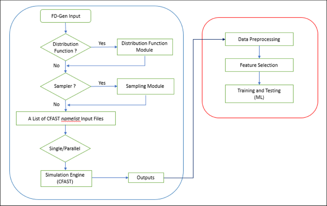
CFAST Fire Data Generator (CData)¹ is a computational tool to generate time series data for typical devices/sensors (i.e. heat detector, smoke detector, and other targets) in any user-specified building environment. There are four fundamental elements associated with CData: 1) basic input handler, 2) distribution function module, 3) sampling module, and 4) simulation engine. It should be noted that the code is written to execute multiple runs with different configurations on the Fire Research Division computer cluster at NIST in parallel. Depending the availability on the computational resources, a maximum of ten thousand simulation cases can be completed in a single day.

Basic input handler

The growth and the spread of a fire depend on many factors. For CData, the basic input handler is capable of handling input parameters accounting for the effects associated with different geometric and/or thermal configurations for the building and various types of fires. Table 1 provides the overall statistics and the assumed distribution functions for a list of important parameters that are found in a previous study associated with residential buildings [19]. Users can utilize the information from the table as the range of inputs to configure the simulation cases. User-specified values will be needed in case of missing statistics or assumed distribution functions.

Table 1:

Statistics on selected CData input parameters for residential buildings.

Parameter	Units	Min	Mean	Max	Assumed Distribution Function
Floor area	m2	12.8	18.2	34.6	Lognormal
Ceiling height	m	2.13	2.61	3.66	Lognormal
Opening width	m	0.81	2.03	3.24	Lognormal
Opening height	m	1.93	2.27	NA	Lognormal
Wall conductivity	W/m-K	NA	1.03	NA	NA
Wall thickness	mm	13.5	14.3	15.9	Lognormal
Fire location2	--	1	2	4	Normal

In addition to the parameters shown in the table, other input parameters include: a) the opening condition, wall density and wall specific heat of the buildings; b) the peak HRR, total energy and its plateau for fires; and c) the thermal properties, locations, and the normal direction for detectors. For commercial buildings, the current version of CData does not have the statistics and the assumed distribution functions for any input parameters. For that, user-specified values are required. However, this information can be obtained from [20] and might be considered in the future updates.

Distribution function module

In order to produce sampling values of the input parameters based on their assumed probability distribution, SciPy [21] is implemented. SciPy is a module written in Python that consists of a library with well-known probability distribution functions. In the current version, the code can account for the following univariate distributions such as Binomial, Exponential, Logistic, Lognormal, Normal, Poisson, Triangular, Uniform, Weibull, Gamma, and Beta. Based on recent literature [21], the Normal, Lognormal, and Uniform distribution functions will mostly be used. The mathematical formulation of these distribution functions is provided below and Figures 1 show the profiles for the 3 distribution functions for reference:

$$Normal(x;\mu ,\sigma )=\frac{1}{\sigma \sqrt{2\pi }}{e}^{-\frac{{(x-\mu )}^2}{2{\sigma }^2}}$$ (1)

$$Lognormal(x;\mu ,\sigma )=\frac{1}{x\sigma \sqrt{2\pi }}{e}^{-\frac{{[\ln (x)-\mu ]}^2}{2{\sigma }^2}}$$ (2)

$$Uniform\left(x;y_0,y_1\right)=\frac{\left[G\left(x-y_0\right)-G\left(x-y_1\right)\right]}{y_1}$$ (3)

Figures 1:

Profile for the 3 distribution functions with given μ, 𝜎, y₀, and y₁.

Sampling module

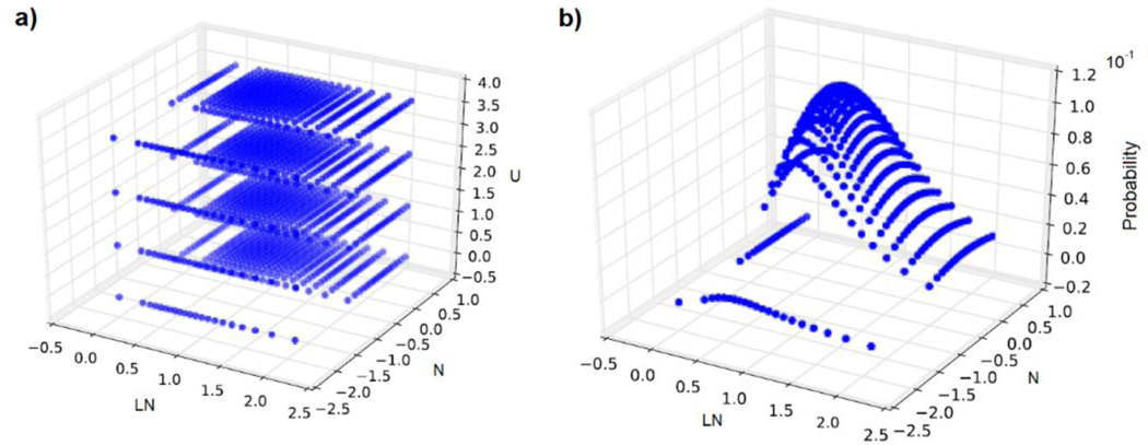
In CData, a sampler connects a set of variables to their corresponding distributions and produces a sequence of points in the input space. This is an important feature for CData as it would greatly affect the cost of computational resources. For this current version, the code only supports 1 sampler and it is the grid sampler. Using Eqns. 1 to 3 with μ, 𝜎, y₀ and y₁ being 0, 0.5, −3, and 3, respectively, Figures 2 show the sampling coverage in 3-D space. For the grid sampler with 20 points over the Normal and Lognormal distributions and 4 points over the uniform distribution spaced in the variable values, 1600 sampling points will be needed. In the future, Monte Carlo and/or Latin Hypercube Sampling can be implemented to provide the sampling flexibility and enhance numerical efficiency.

Figures 2:

a) 3-D dispersion of the sampling point coordinate and b) the probability map.

Simulation engine

CFAST [22] is used as the simulation engine for CData. In general, CFAST is a fire simulation program that divides compartments into two zones. Each zone includes a gas mixture/soot medium bounded by a ceiling or a floor, and four surfaces. Thermal conditions of each zone are assumed to be uniform. When there is a fire, a hot layer will form and the medium can be divided into an upper layer and a lower layer. If the fire persists, the upper layer increases in depth and the temperature will rise. When openings exist, there will be natural flow through the openings allowing air exchange between different compartments and zones. Figure 3a shows a typical simulation case with a user-specified fire in a zone for 3-compartments building structure.

Figures 3:

a) Visualization of a typical CFAST simulation and b) exploded view for detectors.

In CFAST, devices, such as heat detectors, smoke detectors, and other targets can be specified. Although the CFAST simulation is based on the zone method, empirical equations are implemented to determine the local parameters such as gas temperature, smoke concentration, and total radiative heat transfer for heat detectors, smoke detectors, and other targets, respectively. Most importantly, CFAST is verified and validated such that the simulation results obtained from the program are reliable for a wide range of input conditions. Physically, verification ensures a given model is translated correctly into the computer program, and validation ensures the model accurately represents the phenomena of interest. Appendix A provides the full validated range of input parameters and Appendix B shows the modeling uncertainty for all output quantities of interest. Based on Appendix B, it is worth noting that CFAST is conservatively biased, in comparison to the experimental data, for all output quantities except those underlined fonts. In summary, Figure 4 presents the overall workflow for CData.

Figure 4:

The workflow for CData and the workflow for machine learning model development.

Machine Learning Paradigms

Machine learning (ML) algorithms have been widely used for multi-class classification problems in various fields. Based on recent literature [23–26], it has been demonstrated that support vector machine (SVM), decision tree (DT), and random forest (RT) have the capabilities to handle complex time series data with multi-dimensional feature vectors. While guidelines for the use of ML algorithms for classification problems involving time series data in fire research are lacking, the performance for 3 ML algorithms is unknown. For that, SVM, DT, and RF will be used for the development of classification models for prediction of fire hazards. It can be shown that result comparison between different models can serve as a sanity check for the performance of each model. In the next subsection, the basic concepts for SVM, DT, and RT will be presented. Readers can refer to the following references [27–29] for detailed descriptions of the mathematical formulation for each algorithm. It should be noted that ML algorithms such as support vector regression [27] and regression tress [28] can be used for regression problems.

Support Vector Machine (SVM) [27]

SVM is a classifier that finds a decision boundary, known as hyperplane, to separate instances from two classes and maximizes the constrained margin such that the distance between the instances for different classes is optimal to achieve greatest model generalizability. For example, given a training dataset 𝑇 = {(𝑋₁, 𝑦₁), (𝑋₂, 𝑦₂), …, (𝑋_𝑛, 𝑦_𝑛)} which can be linearly separated, the hyperplane denoted as 𝑝 can be written as:

$$w·X+b=0$$ (4)

where 𝑋_𝑛 is the sample of 𝑛^𝑡ℎ instance and 𝑦_𝑛 is the class label. The parameter 𝑤 and 𝑏 is the weight and the bias of the hyperplane, respectively. Based on the definition provided in [27], the distance between the instances for different classes is:

$$d=\underset{i=1,2,\dots ,n}{\min }{y}_i\left(\frac{w}{\parallel w\parallel }\cdot X_i+\frac{b}{\parallel w\parallel }\right)$$ (5)

where ‖𝑤‖ is norm of 𝑤. For SVM, the distance is known as margin. Therefore, SVM determines the hyperplane with the largest margin by solving the optimization problem:

$$\underset{w,b}{\arg \max }\left(\underset{i=1,2,\dots ,n}{\min }{y}_i\left(\frac{w}{\parallel w\parallel }\cdot X_i+\frac{b}{\parallel w\parallel }\right)\right)$$ (6)

For real-life applications, fire data are often more complex and they are not linearly separable. There are two treatments to overcome the numerical difficulty. The first treatment is called the “kernel trick” [27] and there are 4 commonly used nonlinear kernel functions: 1) polynomial kernel, 2) Gaussian kernel, 3) radial basis function, and 4) sigmoid kernel. The use of a kernel function allows the transformation of data into a higher dimensional space such that the instances 𝑋_𝑛 for different classes in which a hyperplane exists. The second treatment is to introduce a regularization/slack variable. With the implementation for the regularization variable, a small proportion of the data are ignored and misclassification is allowed. Although there is trade-off for use of this treatment, it generally helps to avoid over-fitting and provides a more generalized model.

Decision Tree (DT) [28]

DT builds classification models in the form of a tree structure. A typical DT is composed of a root node, internal nodes, edges, and leaves. The root node represents the entire population. Internal nodes represent partitioning/splitting conditions corresponding to a feature vector and edges can be a specific value or range of values for the splitting condition of the feature. The leaves represent the terminal nodes of a tree with class labels. The hierarchical nature of the algorithm provides detailed information of how a decision is being made. As compared to SVM, DT is more transparent and the results are easier to interpret.

Given the abovementioned training dataset 𝑇 = {(𝑋₁, 𝑦₁), (𝑋₂, 𝑦₂), …, (𝑋_𝑛, 𝑦_𝑛)}, the formulation of a DT involves selecting optimal splitting features. The process starts by splitting the dependent feature, or the parent node (root), into binary pieces, where the child nodes are ‘purer’ than the parent node. For DT, the measure of impurity can be characterized by entropy. If the sample is completely homogeneous, the entropy is zero whereas if the sample is equally divided, it has entropy of one. Mathematically, entropy is defined as:

$$Entropy=-\sum _{i=i}^k{P}_{k}log{P}_k$$ (7)

where 𝑃_𝑘 is possibility of the instance belonging to class 𝑘. In general, DT searches through all candidate splits to find the optimal split that maximizes the “purity” of the resulting tree (as defined by the largest decrease in the impurity). One effective split strategy is to always select the feature with largest information gain, 𝐼𝐺:

$$IG\left(D_p,f\right)=Entropy\left(D_p\right)-\sum _i^{all child node}\frac{N_i}{N}Entropy\left(D_i\right)$$ (8)

where 𝐷_𝑝 is the dataset of the parent node with 𝑁 number of samples, 𝑓 is the feature, and 𝐷_𝑖 is the dataset of the 𝑖^𝑡ℎ child node with 𝑁_𝑖 number of instances. This splitting process is continued until all the instances at current level are labeled to the appropriate classes.

Random Forest (RF) [29]

RF is an ensemble learning method for classification. It builds 𝐻 number of classifications trees and provides prediction of the class of an object based on the averaged results obtained from each of the trees. Mathematically, after 𝐻 trees are grown, the RF classification predictor is given as:

$$f(x)=\frac{1}{H}{\sum }_{i=1}^{H}K(i,x)$$ (9)

where 𝑥 is the input feature.

Results and Discussion

Consider a single-story building with three compartments similar to that shown in Figure 3a. There are two offices and one corridor. The dimensions of the two offices are identical and they are 8 m x 4 m x 3.5 m for length, width, height, respectively. The corridor dimensions are 3 m x 8 m x 3.5 m. The material of the surfaces, ceiling, and floor is concrete. The office located in the upper left-hand corner is denoted as Office1 and the other office is denoted as Office2. It can be shown that there are 3 openings: one is in between Office1 and corridor, one is in between Office2 and corridor, and one is connected for corridor and the outdoor environment. The dimensions of the three openings are 2m in width and 1m in height. Initially, the openings are all closed, when the normal incident heat flux to the center of the opening is greater than 2.5 kW/m², the opening will then be opened. Heat detectors are located at the center of the ceiling in each compartment. The outdoor conditions are normal with the temperature maintained at 20 °C at 100 kPa.

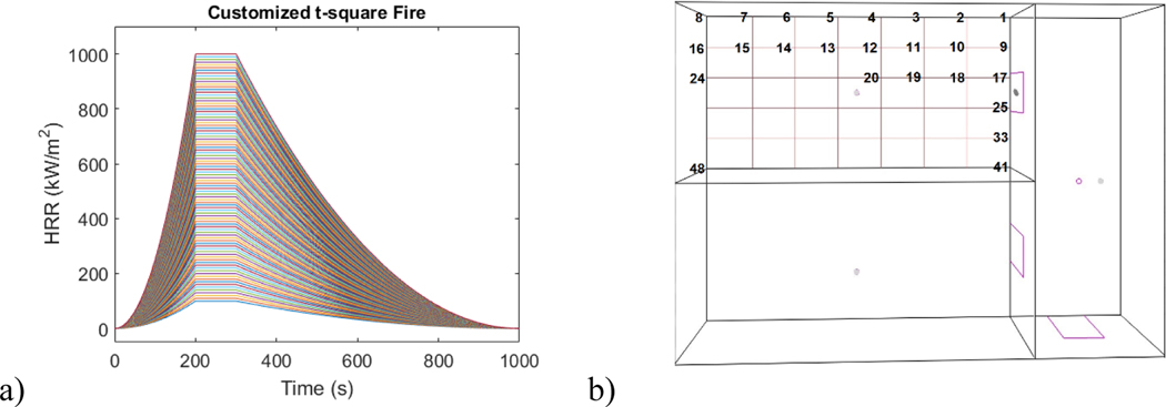
Given the compartment settings provided above, simulation runs are executed for a fire with a wide range of peak heat release rates (HRRs) at different locations in Office1. Figure 5 shows the profile of 1000 HRR curves for fires and the 48 locations of a fire with a given HRR curve. Using a t-square relationship provided in CFAST and the limits of peak HRR (i.e. the lower bound to be 100 kW and the upper bound to be 1000kW), the varying HRR curves can be generated using grid sampling (with 10 kW increment) on peak HRR. Similarly, since the floor dimensions of Office1 are specified, the 48 locations of a fire with the HRR curve are generated using the grid sampler. It can be seen that 8 fire locations are specified in the horizontal direction and 6 fires are specified in the vertical direction. In total, detector temperature for 4800 simulation runs are obtained. The simulation time is set for 3600 s and output intervals are set to be 1 s. For this example, the total computational time is approximately 1.5 h.

Figures 5:

a) 100 t-square fire profiles and b) 48 fire locations in Office1.

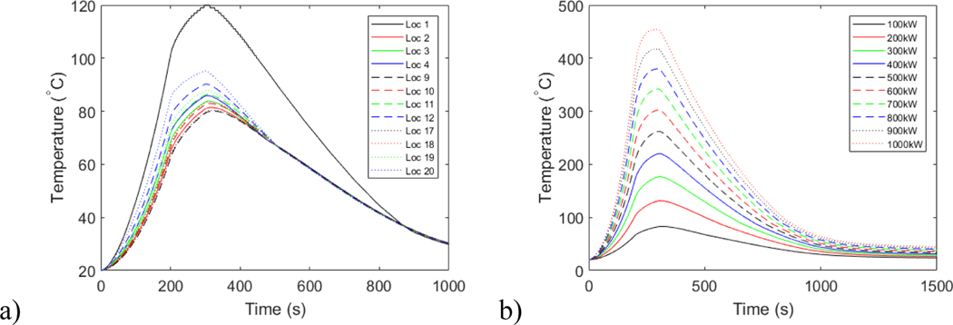
Figures 6 show the detector temperature profiles for a 100 kW peak HRR fire for all 48 locations in Office1 and the detector temperature profiles for all t-square fires at a location. The relative distance in between the fire location and detector location is 1.71 m in horizontal direction and 1.20 m in vertical direction (Loc 10). In Figure 6a, that peak detected temperature for Loc 1 is the highest. The observation is probably due to the corner effect associated with the fire.

Figures 6:

Temperature profiles a) for a fire with 100 kW peak HRR at different locations and b) for fires with different HRR ranging from 100 kW to 1000kW at Loc 10.

Machine Learning Model Development

Given a synthetic dataset, the use of the machine learning paradigm requires four additional processes: 1) preprocessing, 2) feature extraction, and 3) training, and 4) evaluation. Since the focus of this paper is on CData, only a brief discussion on the use of the machine learning paradigm will be included. It should be noted that the information provided in the subsections is only for demonstration. For simplicity, the example below would only take into account the data generated for cases with the same HRR profile (100 kW in Figure 6b) for 48 different fire locations (refer to Figure 5b). In total, the dataset contains detector temperature profiles for 48 simulation runs.

Preprocessing

There are three important matters that the data preprocessing will have to consider in this example case. The first one is to categorize target labels such that a machine learning model can be trained efficiently. Figure 6a shows that the change of detector temperature profiles depends primarily on the relative distance between the fire and the detector. The figure shows the closer the fire to the detector, the higher the maximum detector temperature. An exception is observed for the case with a corner fire. Physically, this is due to the corner effect of the fire that yields a ceiling jet with much higher temperatures. Based on the data behavior obtained from the data analysis and numerical experiment, the target labels for the current dataset will be modified and categorized into different “classes”. Table 2 shows the breakdown information about the new labels. For labels in Class 1, the fire is located in a distance ranging from 0 m to 1 m.

Table 2:

New labels for the example dataset.

Labels	Location Range (m)	Number of profiles
Class 1: very close to the detector	0 – 1	2
Class 2: close to the detector	1 – 2	4
Class 3: a distance from the detector	2 – 3	6
Class 4: far away from the detector	3 – 4	6
Class 5: very far away from the detector	4 – 4.75	4
Class 6: at corner	4.75	2

The second matter is the removal of duplicate information in the dataset. As shown in Figure 5b, symmetry along the centerline across the horizontal direction of Office1 is observed. Since CFAST is a zone model with the identical boundary and initial conditions for the cases, the resulting detector temperature profiles for two separate fire cases (even with same HRR profile) at two different locations (i.e. Loc 12 and Loc 28) will be identical. This type of duplicate information is problematic when a machine learning model is being evaluated for prediction accuracy. Physically, this can be explained with the fact that a well-trained model based on a dataset will have perfect predictions (~100 % accuracy) when applied to a dataset used for training. However, when the model is applied, the prediction accuracy for such model might be very low. This behavior is considered as overfitting. To counter overfitting, unseen data will have to be used for testing [30]. For that, only data associated with fire locations from Loc 1 to Loc 24 will be considered.

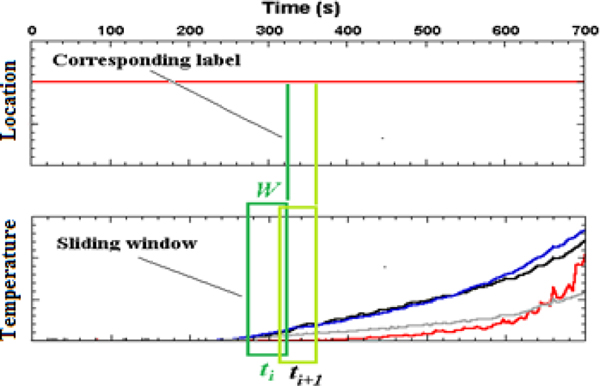
Lastly, a segmentation on the dataset is required for real-time applications. Specifically, the entire detector temperature profile for a specific case as shown in Figure 6a will have to be divided into smaller time series as shown in Figure 7. It can be understood that a machine learning model will be able to encode more precise information (i.e. trend, rate or change, etc.) about the fire using the entire detector temperature profile as an instance for a feature vector. In this scenario, it is highly likely that the model will have better prediction performance. However, such model would lose the ability of real-time detection, as it needs to wait for the complete temperature profile. In this example, 3600 s of data are needed. In order to build a model that is feasible to be used in real-time, the dataset is suggested to be divided into smaller segments using a rolling time window. In this scenario, only partial information about the temperature profile will be needed. In this pilot study, a parametric study will be carried out to examine the prediction performance for different lengths of the time window, W. The window size will vary from 0 s to 120 s (with increment of 10 s).

Figure 7:

Schematic of moving windows with window size, 𝑊, and its corresponding label.

Feature Extraction

Feature extraction is a critical process for obtaining feature vectors that can include important information about the data. A good feature extraction will also help increase the prediction performance for a machine learning model. In this example, we aim to extract features based on the temperature profiles for fire location detection. For each fire event, we describe the temperature signal as: 𝑇 = [𝑇₁, 𝑇₂, …, 𝑇_𝑛], where 𝑇_𝑖 is the detected temperature at time stamp, t, of 𝑖. In addition, we further extract speed signal: 𝑆 = [𝑇₁/𝑡₁, 𝑇₂/𝑡₂, …, 𝑇_𝑛/𝑡_𝑛 ], which indicates the average temperature growth rate (°C⁄𝑠) and the time, 𝑡, is the window size. Statistical features such as maximum and mean of these signals are also extracted. Moreover, since the data is given in time series, the first order derivatives of these signals are also considered. Table 3 summarizes the signals and features that will be used in our model.

Table 3:

Signals and their features.

Signal	Features
Temperature	Maximum, mean, median
Speed
First order derivative of Temperature
First order derivative of Speed

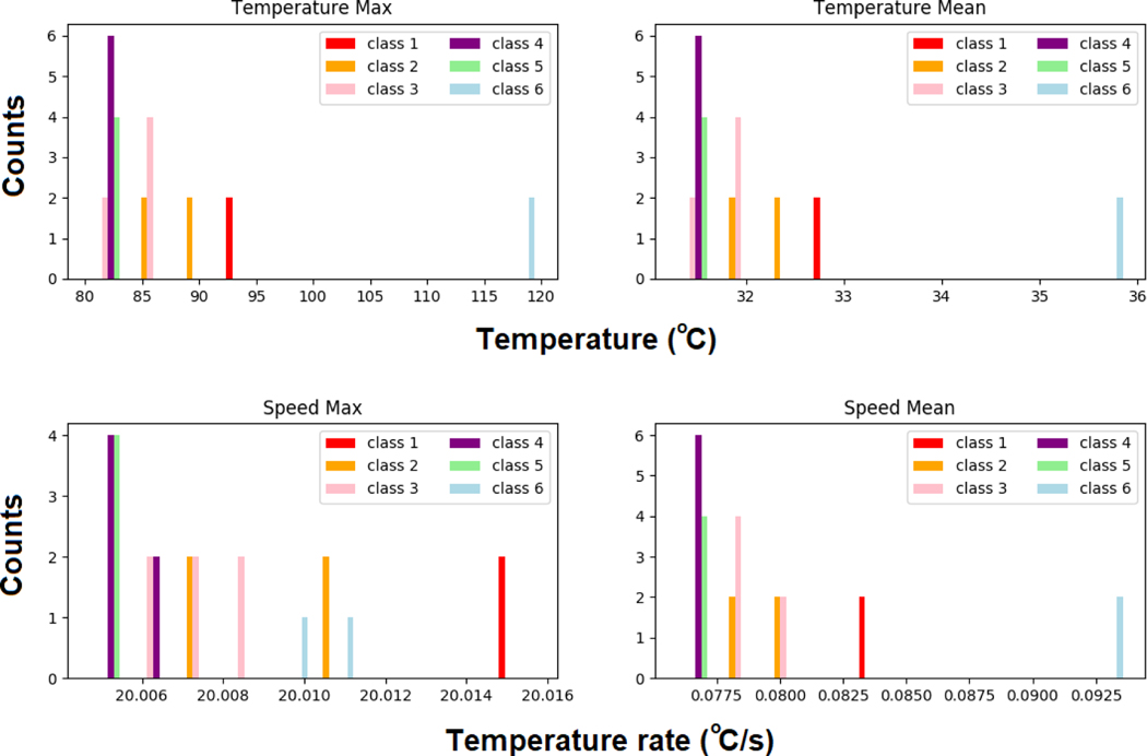
Figure 8 shows the data distribution for the statistical (max and mean) temperature and speed signals based on the entire time series and four distinct behaviors are observed. It can be seen that 1) the fire located at the corner (Class 6) has a much larger maximum (refer to upper left plot) and average temperature (refer to upper right plot). The fire that is very close to the detector (Class 1) has the largest maximum temperature growth rate (refer to lower left plot). And for the fire that is far (Class 4) and very far away (Class 5) from the detector, they both have a lower maximum and lower average temperature (refer to upper plots). Cases associated with fire of Class 5, however, tend to have lower average temperature growth rates than that of Class 4.

Figures 8:

Data distribution for scenarios using the entire profile.

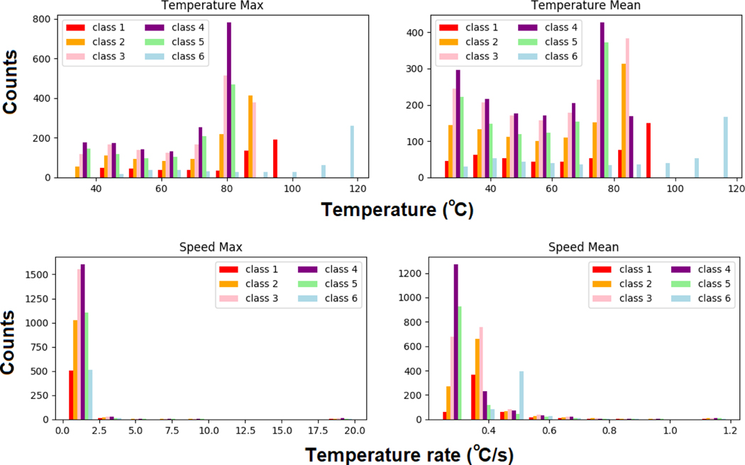
Figure 9 shows the data distributions for the statistical signals for temperature and speed segmented based on the rolling window technique. In this figure, the window size is 120 s. Similar to that of seen in Figure 8, clear distinctions associated with each feature are observed. For this purpose, it can be expected that the use of these features for building a model will likely lead to good performance.

Figures 9:

Data distributions for scenarios with real-time detection (W = 120 s).

Training and Evaluation

With the preprocessed data and the extracted features, classification models can be trained using the 3 different algorithms: SVM, DT, and RF. In this study, scikit-learn is used to facilitate the model training as well as model evaluation. Scikit-learn [31] is open-source machine learning library. It provides a range of supervised learning algorithms through a consistent interface in Python [32]. The algorithms, for example, include support vector machine, decision tree, random forest, gradient boosting, k-means, etc. Since the vision for the library is a level of robustness and support required for use in production systems, considerations, such as ease of use, code quality, collaboration, documentation and performance, are of the primary focuses. It should be noted that another advantage of utilizing the scikit-learn is that the algorithms provided in the library are well maintained and regularly updated such that the algorithms are optimized, verified, and validated.

In general, a significant effort is usually needed for model tuning to maximize a model performance. This process can be accomplished by selecting appropriate hyperparameters³ and there are several automated tuning methods, such as grid search, random search, and Bayesian optimization. In this study, the most basic tuning method, grid search [33], is used. With this technique, we simply build a model for each possible combination of all of the hyperparameter values provided, evaluating each model, and selecting the architecture which produces the best results.

Table 4 provides the summary of model configurations for the 3 ML algorithms. For SVM, radial basis functions kernel (RBF) function is used. The selection of the kernel function depends on both the number of input features and the size of the dataset. In this study, there are a maximum of 12 features and roughly 23,760 instances⁴. Since the number of samples from the dataset is much larger than the number of input features, it is suggested that RBF tends to have better performance [34]. With the use of RBF kernel, the two parameters, 𝐶 and 𝛾, must be considered. The parameter 𝐶 is the regularization parameter/slack variable and it trades off misclassification of training examples against simplicity of the decision surface. In general, a low 𝐶 makes the decision surface smooth, while a high 𝐶 aims at classifying all training examples correctly [29]. The parameter 𝛾 defines how much influence a single training example has. The larger 𝛾 is, the closer other examples must be to be affected. Grid search [33] is used to determine the optimal values for the two parameters.

Table 4:

Summary of model configurations for SVM, DT, and RF.

SVM				DT	RF
	Optimal	Range	Interval			Optimal	Range	Interval
C	100	0 – 300	10	NA	Estimator	10	5 – 100	5
Gamma (𝛾)	10	0 – 50	1

The model configurations for DT and RF are simpler. For DT, entropy method is used to measure the quality of a split, but no parameters were needed to be adjusted. For RF, the setting remains similar except that the optimal number of trees is required to be identified. In theory, the more the number of the trees, the prediction is less biased. However, based on results obtained for different number of trees ranging from 10 to 100 with an interval of 10 trees, the improvement of prediction accuracy for having more trees is negligible (less than 0.1 %). Therefore, the number of trees is determined to be 10.

For evaluation purposes, we divide the dataset into two subsets: a training set and a testing set. We train the detection model based on the training set and evaluate the performance of the model using the testing set. Since the dataset for this example is relatively small, we adopt leave-one-experiment-out cross-validation to evaluate our model. Specifically, we divide the dataset into 24 subsets where each subset contains only the data instances from one particular simulation run. We then train the classifier with the 23 sets among them (the training set) and carry out evaluation on the remaining one (the testing set). This is repeated 24 times for all subsets. The overall average accuracy across the 24 evaluations is reported as the final performance.

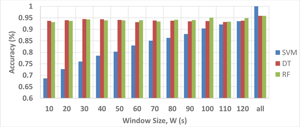
Figure 10 shows the model performance for the classification of fire relative locations associated with SVM, DT, and RF in two window size settings. For the scenario using the entire temperature profiles (denoted as W = all), results indicate that the 3 machine learning models are capable to classify the fire relative locations with reasonable accuracy. No misclassification is observed for SVM. The accuracy⁵ associated with DT and RF is 95.83 % and only one instance is wrongly classified in which a Class 2 (close to the detector) instance is wrongly detected as Class 3 (medium distance to the detector). For scenarios using the rolling window technique, the window size does not have significant impacts on DT and RF models and the model performance varies in between 93 % to 95 % with the best performance observed to be 95.08% (W = 100 s using RF). In contrast, SVM has a decreasing performance with decreasing window size and the model needs at least 100 s of data to have model accuracy above 90 %. However, it is believed that the model performance will be improved if there are more data. Nevertheless, the current results demonstrate that DT and RF are more applicable to detect fire relative locations in real-time situations.

Figures 10:

Performance of fire location detection for the scenario of using the entire profile (𝑊 = 𝑎𝑙𝑙) and the scenario of real time detection (𝑊 > 0𝑠).

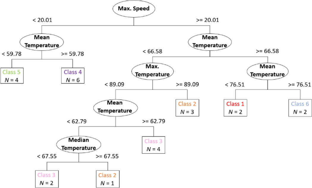
Figure 11 shows a tree diagram obtained from DT for the classification task considering instances consisted of entire temperature profiles (𝑊 = 𝑎𝑙𝑙). The tree diagram provides 2 important pieces of information: 1) features being used for splitting and 2) threshold values for each splitting. Based on the tree diagram, features including maximum speed, mean temperature, maximum temperature, and median temperature are being used to distinguish the different class of labels. For example, the model predicts the fire will be approximately 4 m to 4.75 m away from the detector (Class 5) if the maximum speed and mean temperature is smaller than 20.01 °C/s and 59.78 °C, respectively. It is worth noting that the classification for Class 2 and Class 3 is more complex. For Class 2, the model needs additional features and conditions to better distinguish Class 2 from Class 3 for some of the instances. Nevertheless, it can be demonstrated that classification models developed using DT is more transparent as compared to algorithms, such as SVM, and the results obtained from DT are easier to interpret.

Figures 11:

Tree diagram for DT model for classification of relative fire locations for 24 entire time series as the input feature (𝑊 = 𝑎𝑙𝑙)

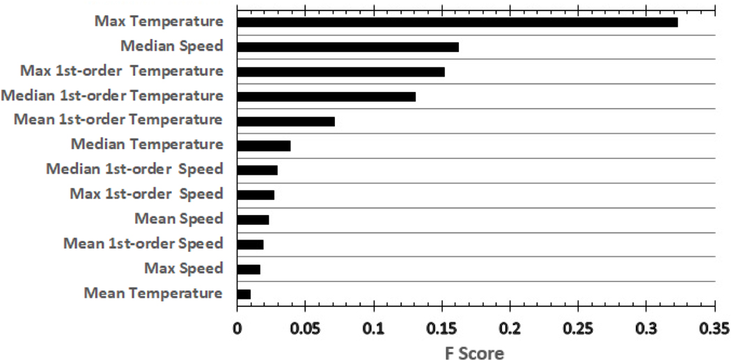
Figure 12 shows the use of RF to evaluate the importance of features⁶ for a classification task considering instances with 120 s of temperature data. Unlike tree diagrams, this technique does not provide specified information associated with the features and conditions being used in one tree, it offers a global insight to the model by averaging the information obtained from a desired number of trees (i.e. 10 trees). As shown in Figure 12, all of the features are being ranked. For feature importance, the higher the value is, the more important the feature. In this classification task, it can be seen that maximum temperature has the highest score, following by median speed, maximum first order temperature, and median first order temperature. If a much larger dataset exists, attempts can be made to train the classification model with 4 of the most effective features. By doing so, the training time can be significantly reduced while maintaining the same order of model accuracy.

Figures 12:

Feature importance obtained from RF for classification with partial temperature profiles (𝑊 = 120 s).

Conclusions

The workflow for the CFAST Fire Data Generator (CData) is presented. The functionalities associated with the basic input handler, distribution function module, sampling module, and simulation engine are discussed. Using CData, synthetic data for heat detector temperature are obtained for 4800 cases in a single-story building with three compartments. As a demonstration, these data are used to train 3 machine learning algorithms. Data preprocessing is carried out to remove duplicate information in the dataset. Simple features are obtained to facilitate the model training. Results show that the proposed models can predict the relative location of the fire with reasonable accuracy. Based on a parametric study, the selection of a particular data window size does not greatly affect the overall performance of the model. Consistent model performance is observed using any window size ranging from 20 s to 120 s. For real-time predictions, using DT and RF with 30 s window size can provide reliable detection of fire location in the example case.

In general, the current work will help to facilitate the development of machine learning models that can enhance the situational awareness for fire fighting.

Appendix A: Summary of important experimental parameters [22].

Test Series	Q (kW)	D (m)	H (m)	$\dot{Q}$*	Ls/H	ϕ	W/H	L/H	rcj/R	rnd/D
ATF Corridors	50 – 500	0.5	2.4	0.3–3 3	0.3–0.9	0.0 – 0.1	0.8	7.1	0.8 – 6.0	N/A
Fleury Heat Flux	100 – 300	0.3 – 0.6	Open	0.3 – 5.5	Open	Open	Open	Open	Open	1.7 – 3.3
FM/SNL	470 – 516	0.9	6.1	0.6 – 2.4	0.3 – 0.6	0.0 – 0.2	2.0	3.0	0.2 – 0.3	N/A
iBMB*	3500, 400	1.l3, 0.79	5.7, 5 6	2.4, 0.7	0.6, 0.4	0.6, 0.l	0.6	0.6		N/A
LLNL Enclosure	50 – 400	0.6	4.5	0.2 –1.5	0.1 – 0.4	0.1 – 0.4	0.9	l.3	0.3 – 1.0	N/A
NBS Multi-Room	110	0.3	2.4	1.5	0.5		1.0	5.1		N/A
NBS Single-Compartment	2900 – 7000	1.1 – 1.7	2.4	1.7 – 2.3	1.1		1.0	1.5		N/A
NIST Seven-Story	1130	0.7	2.6	2.2	1.1		0.7	5.6		N/A
NIST/NRC	350 – 2200	1.0	3.8	0.3 – 2.0	0.3 – 1.0	0.0 – 0.3	1.9	5.7	0.3 – 2.1	2.0 – 4.0
NIST/NRC Cabinet	200 – 400	0.3 – 0.5	2.1	0.3 – 3.7	0.2 – 0.9	1.3 – 12	0.3	0.4	N/A	1.2 – 2.0
NIST/NRC Corner	200 – 400	0.7	3.8	0.4 – 0.9	0.3 – 0.5	<0.1	1.8	2.9	0.5 – 2.3	N/A
NIST Smoke Alarm	100 – 350	1.0	2.4	0.1 – 0.3	0.2 – 0.5		1.7	8.3	1.3 – 8.3	N/A
PRISME	480 – 1600	0.7 – 1.1	4.0	1.1	0.5 – 0.8	0.5	1.3	1.5	0.0 – 0.5	2.3 – 5.7
SP AST	450	0.3	2.4	6.1	1.1	0.1	1.0	1.5		N/A
Steckler	31.6 – 158	0.3	2.1	0.8 – 3.8	0.3 – 0.7	0.0 – 0.6	1.3	1.3		N/A
UL/NFPRF	4400 – 10000	1.0	7.6	4.0 – 9.l	0.7 – 1.0	Open	4.9	4.9	0.6 – 3.9	N/A
UL/NIST Vents	500 – 2000	0.9	2.4	0.7 – 2.6	0.8 – 1.6	0.2 – 0.6	1.8	2.5	1.0 – 2.3
USN Hawai	100 – 7700	0.3 – 2.5	15	0.7 – 1.3	0.1 – 0.4	Open	4.9	6.5	0 – 1.2	N/A
USN Iceland	100 – 15700	0.3 – 3.4	22	0.7 – 1.3	0.0 – 0.3	Open	2.1	3.4	0 – 1.0	N/A
Vettori Flat	1055	0.7	2.6	2.5	1.1	0.3	2.1	3.5	0.8 – 2.9	N/A
VTT Large Hall	1860 – 3640	1.4 – l.8	19	0.7	0.2	0	1.0	1.4	0 – 0.6	N/A
WTC	1970 – 3240	1.6	3.8	0.6 – 0.9	0.8 – 1.l	0.3 – 0.5	0.9	1.8	0.0 – 0.8	0.3 – 1.3

Appendix B: Summary of statistics for all quantities of interest [22].

Quantity	𝜎E	𝜎M	δ
HGL Temperature	0.07	0.32	1 09
HGL Temperature: Forced Ventilation	0.07	0.20	1.13
HGL Temperature: Natural Ventilation	0.07	0.39	1.08
HGL Temperature: No Ventilation	0.07	0.12	0.93
HGL Depth	0.05	0.27	1.01
HGL Depth: Open Compartments	0.05	0.17	0.94
HGL depth: Closed Compartments	0.05	0.24	1.45
Ceiling jet Temperature	0.07	0.45	1.02
Plume Temperature	0.07	0.23	1.08
Carbon Concentration	0.08	0.26	1.03
Carbon Dioxide Concentration	0.08	0.27	0.89
Carbon Monoxide Concentration	0.19	0.65	1.04
Smoke Concentration	0.19	0.68	3.43
Compartment Over-Pressue	0.23	0.56	1.45
Target Temperature	0.07	0.50	1.25
Surface Temperature	0.07	0.21	1.00
Target Heat Flux	0.11	0.60	0.97
Surface Heat Flux	0.11	0.23	0.91
Smoke Alarm Activation Time (Temperature Surrogate)	0.34	0.43	1.23
Smoke Alarm Activation Time (Smoke Obscuration)	0.34	0.51	0.56
Sprinkler Activation Time	0.06	0.20	1.01

Note that the term δ is a calculated bias factor representing the degree to which the model over-predicted or underpredicted experimental data, the term 𝜎_M is a measure of model uncertainty, and the term 𝜎_𝐸 is a measure of experimental uncertainty. The expression δ > 0 means the model over-predicted the observations, and 𝜎_𝑀 < 𝜎_𝐸 means that the model uncertainty is within experimental uncertainty.

References

- [1].Hamins AP, Bryner NP, Jones AW and Koepke GH, 2015. Research Roadmap for Smart Fire Fighting (No. Special Publication (NIST SP)-1191). [Google Scholar]
- [2].Qolomany B, Al-Fuqaha A, Gupta A, Benhaddou D, Alwajidi S, Qadir J. and Fong AC, 2019. Machine Learning, Big Data, And Smart Buildings: A Comprehensive Survey. arXiv preprint arXiv:1904.01460. [Google Scholar]
- [3].Overholt KJ and Ezekoye OA, 2012. Characterizing heat release rates using an inverse fire modeling technique. Fire Technology, 48(4), pp.893–909. [Google Scholar]
- [4].Lin CC and Wang LL, 2017. Real-time forecasting of building fire growth and smoke transport via ensemble kalman filter. Fire technology, 53(3), pp.1101–1121. [Google Scholar]
- [5].Mahdavinejad Mohammad Saeid, Rezvan Mohammadreza, Barekatain Mohammadamin, Adibi Peyman, Barnaghi Payam, and Sheth Amit P.. “Machine learning for Internet of Things data analysis: A survey.” Digital Communications and Networks 4, no. 3 (2018): 161–175. [Google Scholar]
- [6].Bishop CM, 2006. Pattern recognition and machine learning. springer. [Google Scholar]
- [7].Chenebert A, Breckon TP and Gaszczak A, 2011, September. A non-temporal texture driven approach to real-time fire detection. In 2011 18th IEEE International Conference on Image Processing (pp. 1741–1744). IEEE. [Google Scholar]
- [8].Yin Z, Wan B, Yuan F, Xia X. and Shi J, 2017. A deep normalization and convolutional neural network for image smoke detection. Ieee Access, 5, pp.18429–18438. [Google Scholar]
- [9].Shen D, Chen X, Nguyen M. and Yan WQ, 2018, April. Flame detection using deep learning. In 2018 4th International Conference on Control, Automation and Robotics (ICCAR) (pp. 416–420). IEEE. [Google Scholar]
- [10].Aslan S, Güdükbay U, Töreyin BU and Çetin AE, 2019. Deep Convolutional Generative Adversarial Networks Based Flame Detection in Video. arXiv preprint arXiv:1902.01824. [Google Scholar]
- [11].Zhao Y, Ma J, Li X. and Zhang J, 2018. Saliency detection and deep learning-based wildfire identification in UAV imagery. Sensors, 18(3), p.712. [DOI] [PMC free article] [PubMed] [Google Scholar]
- [12].Celik T, Demirel H, Ozkaramanli H. and Uyguroglu M, 2007. Fire detection using statistical color model in video sequences. Journal of Visual Communication and Image Representation, 18(2), pp.176–185. [Google Scholar]
- [13].McGrattan K, Hostikka S, McDermott R, Floyd J, Weinschenk C. and Overholt K, 2013. Fire dynamics simulator user’s guide. NIST special publication, 1019(6). [Google Scholar]
- [14].Yuen RK, Lee EW, Lo SM and Yeoh GH, 2006. Prediction of temperature and velocity profiles in a single compartment fire by an improved neural network analysis. Fire safety journal, 41(6), pp.478–485. [Google Scholar]
- [15].Hodges JL, Lattimer BY and Luxbacher KD, 2019. Compartment fire predictions using transpose convolutional neural networks. Fire Safety Journal, 108, p.102854. [Google Scholar]
- [16].Lattimer BY, Hodges JL and Lattimer AM, 2020. Using machine learning in physics-based simulation of fire. Fire Safety Journal, p.102991. [Google Scholar]
- [17].Sharma J, Granmo OC, Goodwin M. and Fidje JT, 2017, August. Deep convolutional neural networks for fire detection in images. In International Conference on Engineering Applications of Neural Networks (pp. 183–193). Springer, Cham. [Google Scholar]
- [18].Lichman M, 2013. UCI machine learning repository. [Google Scholar]
- [19].Bruns MC, 2018. Estimating the flashover probability of residential fires using Monte Carlo simulations of the MQH correlation. Fire technology, 54(1), pp.187–210. [Google Scholar]
- [20].https://www.eia.gov/consumption/commercial/data/2012/ [Online; accessed 2019-08–26].
- [21].Jones E, Oliphant E, and Peterson P, 2001. SciPy: Open Source Scientific Tools for Python, http://www.scipy.org/ [Online; accessed 2019–08-26].
- [22].Peacock RD, Reneke PA and Forney GP, 2017. CFAST–Consolidated Model of Fire Growth and Smoke Transport (Version 7) Volume 2: User’s Guide. NIST Technical Note 1889v2. [Google Scholar]
- [23].Mishra Manohar, and Pravat Kumar Rout. “Detection and classification of micro-grid faults based on HHT and machine learning techniques.” IET Generation, Transmission & Distribution 12, no. 2 (2017): 388–397. [Google Scholar]
- [24].Kazem Hussein A., Yousif Jabar H., and Chaichan Miqdam T.. “Modeling of daily solar energy system prediction using support vector machine for Oman.” International Journal of Applied Engineering Research 11, no. 20 (2016): 10166–10172. [Google Scholar]
- [25].Moutis Panayiotis, Spyros Skarvelis-Kazakos, and Maria Brucoli. “Decision tree aided planning and energy balancing of planned community microgrids.” Applied energy 161 (2016): 197–205. [Google Scholar]
- [26].Jiang Huaiguang, Li Yan, Zhang Yingchen, Jun Jason Zhang David Wenzhong Gao, Muljadi Eduard, and Gu Yi. “Big data-based approach to detect, locate, and enhance the stability of an unplanned microgrid islanding.” Journal of Energy Engineering 143, no. 5 (2017): 04017045. [Google Scholar]
- [27].Vapnik Vladimir. “The support vector method of function estimation.” In Nonlinear Modeling, pp. 55–85. Springer, Boston, MA, 1998. [Google Scholar]
- [28].Breiman Leo. Classification and regression trees. Routledge, 2017. [Google Scholar]
- [29].Breiman Leo. “Random forests.” Machine learning 45, no. 1 (2001): 5–32. [Google Scholar]
- [30].Schittenkopf C, Deco G. and Brauer W, 1997. Two strategies to avoid overfitting in feedforward networks. Neural networks, 10(3), pp.505–516. [Google Scholar]
- [31].Pedregosa Fabian, Varoquaux Gaël, Gramfort Alexandre, Michel Vincent, Thirion Bertrand, Grisel Olivier, Blondel Mathieu et al. “Scikit-learn: Machine learning in Python.” Journal of machine learning research 12, no. Oct (2011): 2825–2830. [Google Scholar]
- [32].Oliphant Travis E. “Python for scientific computing.” Computing in Science & Engineering 9, no. 3 (2007): 10–20. [Google Scholar]
- [33].Staelin Carl. “Parameter selection for support vector machines.” Hewlett-Packard Company, Tech. Rep. HPL-2002–354R1 (2003). [Google Scholar]
- [34].Jebara Tony. “Multi-task feature and kernel selection for SVMs.” In Proceedings of the twenty-first international conference on Machine learning, p. 55. ACM, 2004. [Google Scholar]