In Situ Classification of Cell Types in Human Kidney Tissue Using 3D Nuclear Staining

Abstract

To understand the physiology and pathology of disease, capturing the heterogeneity of cell types within their tissue environment is fundamental. In such an endeavor, the human kidney presents a formidable challenge because its complex organizational structure is tightly linked to key physiological functions. Advances in imaging-based cell classification may be limited by the need to incorporate specific markers that can link classification to function. Multiplex imaging can mitigate these limitations, but requires cumulative incorporation of markers, which may lead to tissue exhaustion. Furthermore, the application of such strategies in large scale 3-dimensional (3D) imaging is challenging. Here, we propose that 3D nuclear signatures from a DNA stain, DAPI, which could be incorporated in most experimental imaging, can be used for classifying cells in intact human kidney tissue. We developed an unsupervised approach that uses 3D tissue cytometry to generate a large training dataset of nuclei images (NephNuc), where each nucleus is associated with a cell type label. We then devised various supervised machine learning approaches for kidney cell classification and demonstrated that a deep learning approach outperforms classical machine learning or shape-based classifiers. Specifically, a custom 3D convolutional neural network (NephNet3D) trained on nuclei image volumes achieved a balanced accuracy of 80.26%. Importantly, integrating NephNet3D classification with tissue cytometry allowed in situ visualization of cell type classifications in kidney tissue. In conclusion, we present a tissue cytometry and deep learning approach for in situ classification of cell types in human kidney tissue using only a DNA stain. This methodology is generalizable to other tissues and has potential advantages on tissue economy and non-exhaustive classification of different cell types.

1 |. INTRODUCTION

Tissue organs in the human body are made up of cells that are highly specialized and organized into functionally important architectures. Identifying the various types of cells and their spatial organization within the tissue is essential to understand the physiological functions of organs and their dysfunction during disease. For example, the organization of kidney tissue illustrates how distinctly heterogeneous cell types work harmoniously to achieve blood filtration and homeostasis and how alteration in function can induce pathological states during kidney disease (1–4). Although novel technologies such as single cell RNA sequencing provide a new development to classify cell types and subtypes based on transcriptome profiling in disaggregated tissues (5–7), the ability to exhaustively classify various cell types in situ based on imaging data, particularly in the human kidney, is not yet fully developed. The development of imaging analytics including classification techniques is crucial, as preserving the tissue architecture and spatial context of each cell will enhance the ability to interpret how specific cell types are linked to biological function.

Cell identification in tissue specimens can be performed in thin sections using histological stains such as Hematoxylin and Eosin (H&E), or Period acid-Schiff (PAS). These stains label the nuclei of cells distinctly from the cytoplasm, thereby allowing for cell visualization and detection. The identification of cell types in such imaged sections typically depends on the expert eye of a pathologist, although newer computer-aided decision support and machine learning tools have enabled enhanced reproducibility (8, 9). The use of such tools in cell classification has predominantly focused on detection of cancer or unique cell phenotypes (10, 11). Broader application of these machine learning approaches in cell classification requires large training datasets, which are difficult to generate (9). In this setting, it is also difficult to classify cells into multiple subtypes that could be linked to biological functions without the use of specific markers. Therefore, to enhance the feasibility and depth of classification, concurrent staining for multiple markers that are individually unique for specific cell populations is needed. Although such multiplexed staining is possible using immunohisto-chemistry, this approach is typically done using immunofluorescence microscopy because of the availability of established methods of quantitating fluorescence and the ability to multiplex spectrally distinguishable fluorophores for various cell markers in a single section of tissue (12–16). With optical sectioning microscopy, querying cell types based on specific markers could also be expanded to 3-dimensional (3D) space, increasing the ability to assay cellular structure and tissue architecture (13, 17, 18).

Multiplex imaging based on cell markers may offer a path to classify cells in tissues, especially with the availability of tissue cytometry software tools that facilitate the analytical process. For example, we recently described the Volumetric Tissue Exploration and Analysis (VTEA) tool which enables the semi-automated classification of labeled cells in 3D image volumes (13, 17, 19). However, multiplexed imaging and tissue cytometry have several challenges that may limit their utility for comprehensive cell classification in situ. These challenges include a potentially lengthy technical workflow, a requirement for image processing expertise to optimize the analysis, and above all, only a finite number of cell-associated markers can be obtained from a single experiment (17). The scarcity of markers is the most limiting, as each time a new marker is discovered or needed, new experiments on additional tissue sections are required. For sparse tissue such as a kidney biopsy, this could lead to tissue exhaustion. Furthermore, because multiplexing is performed at the experimental level, classification of cells in historical datasets from sparse tissue specimen using prospectively discovered new markers is not feasible using this standard workflow. Therefore, it is beneficial to classify cells independently of the presence of specific cell markers in each experimental condition. Relying on information from a common cell marker easily embedded in the staining process and biologically linked to different cell types in the tissue could substitute the need for specific cell markers.

In this work, we proposed a hypothesis that 3D nuclear staining with 4°,6-diamidino-2-phenylindole (DAPI), a nuclear stain commonly used in most fluorescence imaging methods (20), contains enough information for reliable classification of human kidney cells in situ using a supervised learning framework. This hypothesis is supported by previous in vitro work from multiple investigators showing that nuclear staining can infer functional information about cells (9, 21–23). This is not surprising because healthy cell functions (such as various stages of the cell cycle and gene expression) and injury states are associated with specific patterns of chromatin condensation (23, 24). Furthermore, different cell types may have different shapes of nuclei, which is also captured by nuclear staining (13). To test this hypothesis, we leveraged an enhanced functionality of the VTEA cytometry tool to generate large ground truth datasets from kidney tissue labeled with specific markers and investigated the accuracy of various classification methods.

Our experimental results show that deep learning (DL)-based classification models are able to perform kidney cell classification with a satisfactory accuracy, outperforming other classical supervised classification approaches, and that nuclear morphology can successfully classify most cell types in the cortex of the kidney by DL. Furthermore, our results suggest that 3D data improves the predictive ability of this approach compared to 2D data. In addition, minimal labeled data are needed to classify new specimens, which broadens the use of this technique for fine tuning new experiments. The approach of combining tissue cytometry (VTEA) and DL to generate ground truth library datasets as well as classify and visualize cell types in situ is unique. We anticipate that our methodologies will have an important impact to facilitate comprehensive cell classification and visualization in situ within the kidney and potentially other tissues and may enhance the information obtained from sparsely available human specimens. The datasets and approaches used will be made publicly available.

2 |. METHODS

2.1 |. Ethical Statement

Three deceased donor kidney nephrectomy tissues were used with procedures and protocols in accordance with the ethical standards as set forth in the Declaration of Helsinki of 1975 as revised in 2008 and approved by the Institutional Review Board at Indiana University.

2.2 |. Kidney Tissue Specimens

50 μm sections from OCT frozen kidney cortical specimen were fixed overnight with 4% paraformaldehyde or 50 μm sections were cut by vibratome from 4% paraformaldehyde fixed cortical tissue fragments underwent staining with DAPI and antibodies for the specified markers including: Megalin, LRP2 (cat#ab76969,abcam), Aquaporin-1 (AQP1,clone 1/22, cat# sc-32737, Santa Cruz Biotechnology), Slc12A3 (cat#HPA028748, Sigma), Uromodulin, Tamm-Horsfall protein (cat# AF5144, R&D Systems), CD45 (clone HI30,cat# 304002), CD31 (clone JC/70A cat# NB600–562-R, Novus), Nestin (clone 10C2, cat# 656810, Biolegend), and Cytokeratin-8 (cat# NBP-34267, Novus). All staining was performed in 1X Phosphate buffer saline with 10% normal goat serum and 0.1% Triton X-100 with overnight incubations. All secondaries were raised in goat highly cross-adsorbed and were labeled with Alexa488, Alexa546, Alexa555, or Alexa568, Alexa647. The CD31, CD45, and Nestin antibodies were directly conjugated with Dylight 550, Alexa 488, and Alexa 647, respectively. Stained tissue was mounted under #1.5 coverslips in Prolong Glass allowed to cure for 24–48 h before sealing with nail-polish. Mounted and sealed tissue was stored at 4°C before imaging.

2.3 |. Imaging

Image acquisition was performed in four separate consecutive channels using an upright Leica SP8 Confocal Microscope controlled by LAS X software (Germany). Volume stacks spanning the whole thickness of the tissue were taken using a multi-immersion 20× NA 0.75 objective with Leica immersion oil with 1.0-μm z-spacing and 0.5 × 0.5 μm pixels. Large scale imaging was performed using and automated stage with volumes overlapping by ~10%. Typical imaging times were 4–6 h. Image volumes were stitched using FIJI (61).

2.4 |. VTEA Cytometry

Tissue cytometry was performed using a prerelease version of the FIJI plugin Volumetric Tissue Exploration and Analysis(VTEA) (13) available on GitHub (https://github.com/icbm-iupui/volumetric-tissue-exploration-analysis, which incorporates unsupervised learning approaches into a 3D tissue cytometry workflow (manuscript in preparation). Segmentation: Entire image volumes were imported in VTEA and the nuclei channel was pre-processed to facilitate segmentation by performing denoising, rolling-ball background subtraction and contrast stretching to compensate for attenuation of signal at depth. A modified form of connected components built into VTEA (LSConnect3D), which combines Otsu intensity thresholding, water-shed splitting and connected component merging in 3D was used for segmentation. To facilitate segmentation of mesoscale images, LSConnect3D subdivides the image into user defined volumes to facilitate parallelization during processing. Both a minimum and maximum size restriction was placed on nuclei to mitigate segmentation errors. Following segmentation of the nuclei, a second segmented volume, grow-volume, was defined around each nucleus that extend ~2 pixels for assessing stains associated with a nucleus (13). The pixel values, including mean, upper-quartile mean, standard deviation and/or maximum within the segmented nuclei and/or the grow-volume, were used as features for clustering by X-means implemented in SMILE (http://haifengl.github.io/). Validation of clusters was performed by an expert using VTEA’s mapping of gated cells to the original image volume to demonstrate correct localization of the selected nuclei. Nuclei from gated cells were exported by VTEA as user defined image volumes (pixels from the segmented nuclei in a black background, or with surrounding nuclei/not limited to the segmented pixels, etc.) using a duplicate image volume of the DAPI channel that had not been subjected to the image preprocessing necessary for segmentation. The names of exported datasets and a brief description are given in Supporting Information Table S2 and class representation are given in Supporting Information Table S1. A small subset (<1.7%) of nuclei without context were excluded from NephNuc3D when the segmented nucleus extended outside of the sampling volume.

Image analysis was performed on a dedicated workstation with a Xeon 2245 (8 cores) with 256 GB RAM, 2 × 2 TB NVMe SSDs, a 24 TB RAID, 2× 2080Ti (not linked, 11 GB RAM each, Nvidia) running Windows 10.

2.5 |. Expert Review of Classification

Using the pre-release version of VTEA mentioned above, a manual classification was performed on 177 nuclei. VTEA randomly picked segmented nuclei and presented a cropped image with a highlighted nucleus for an expert to place in predefined classes. VTEA provided an interface to tally these nuclei and import these expert classifications as a feature for comparison with other classification approaches. Balanced accuracy was calculated as given below and the kappa statistic was calculated with the package psych in R.

2.6 |. Data Organization

Training data for this research consisted of approximately 230,000 3D images of nuclei, segmented as described above from three reference tissue specimens. Each grayscale image was 32 × 32 × 7 pixels representing in situ dimensions of 17.3 × 17.3 × 3.9 μm and was centered on the centroid of a nucleus segmented by VTEA. Each pixel value was between 0 and 255 denoting the light intensity of the pixel. Eleven kidney cell classes were identified, and the ground truth class-label of each cell was obtained using VTEA cytometry tools. However, the performance of each learning model was reported by using a condensed set of eight classes; for example, while two separate proximal tubule classes are identified in the labels, classifying a nucleus into either class is recorded as a correct classification.

Three different image data formats, 2D slice, 2D maximum projection, and 3D, were considered. 2D slice (or in-short 2D) was obtained by only using the median slice of each volume. 2D maximum project was obtained by considering the maximum pixel value over the z-axis of that pixel. Each image format can include the surrounding nuclei (“with context”) or only the segmented nuclei of interest (“without context”). Context was excluded to generate images without surrounding nuclei by only including pixels from the nuclear segmentation generated by VTEA. (Supporting Information Table S1 and Fig. S1).The datasets were split into 70% training, 15% validation, and 15% testing for deep learning models and 80% training, 20% testing for Random Forest and SVM training unless otherwise noted.

2.7 |. Preprocessing of Nuclei Prior to Classification

Before feeding an image to the classification algorithm, each image was pre-processed as below. First, each pixel value was normalized using Z-score normalization; if I was the intensity of the original pixel, I′ was the intensity of normalized pixel, μ was the mean intensity and σ was the standard deviation of that pixel across the training images, then I′ = (I − μ)/σ. This transformation made the mean intensity of the dataset to be 0 and the variance to be 1. To accommodate a larger input image, 2D images were also scaled by nearest neighbor from 32 × 32 pixels to 64 × 64 pixels.

2.8 |. k-Fold Cross-Validation

The NephNuc3D with context was randomly split into five versions with 65% training, 15% validation, and 20% for testing. Training was performed on the NephNet3D network five times and the mean balanced accuracy and standard deviation calculated.

2.9 |. Feature Extraction and Classical Supervised Classification Models

Image features that were calculated included Image Statistics, Haralick texture features, Parameter-Free Threshold Adjacency Statistics (PFTAS), Zernike Moments and Spherical Harmonics.

2.9.1 |. Image statistics

The image statistics calculated included range of pixel values, counting the number of pixels greater than Otsu’s threshold, sum, squared-sum, average, root-mean-square, variance, standard deviation, and histogram values for 16 equally spaced bins in the range 0–255. The implementation for all these statistics was done on an ad hoc basis in Python.

2.9.2 |. Haralick, Parameter-free threshold adjacency statistics (PFTAS), and Zernicke features

Haralick texture, PFTAS, and Zernicke features were computed using the python library Mahotas. Thirteen Haralick features were computed per image and returns a 4 × 13 feature vector (four directions) for 2-D images and a 13 × 13 feature vector (13 directions) for 3D images. A fourteenth feature “maximum correlation coefficient” was not computed due to instability. Due to limitations of the API, Zernicke features were calculated only on 2D images.

2.9.3 |. Spherical harmonics

Calculation of spherical harmonics was based on the work of Medyukhina et al. (30). Using the NephNuc3D datasets, the surface of nuclei surface was reconstructed in the form of a mesh of triangles using the marching cubes algorithm (scikit-image v. 0.18. dev0). Next, the x, y, and z coordinates of unique vertices were extracted and converted to polar coordinates. These polar coordinates were used to expand a set of irregularly sampled data points into spherical harmonics using a least squares inversion (SHTOOLS 4.6), adapted from “https://shtools.oca.eu/shtools/public/pyshexpandlsq.html.” The maximum spherical harmonic degree of the output coefficients was set to three. These spherical harmonic coefficients were used to compute rotation-invariant frequency spectrum to be used as static features for classification. These static features of each of the nuclei were used in a Support Vector Machine or Random-Forest classifier.

Two classical supervised classification models were used, Random Forest and Support Vector Machine implemented in Scikit-learn (62) (version 0.22.2) in Python with a maximum number of trees equal to 450. The maximum depth was expanded until all leaves were pure or all leaves contained two or fewer samples.

2.10 |. Deep Learning

A custom-made 3D deep convolution neural network (CNN)-based model was used for the kidney cell classification. Besides preprocessing, which was performed prior to the training, some augmentation steps were performed during training, mainly to prevent overfitting. Each augmentation step had a 30% chance of being applied to an image on every epoch. The augmentation steps were mix of transformation, rotation, flip, and noise injection; the transformations were translation up to eight pixels in x- and y-axes and three pixels in z-axis, random rotation up to 35°, random 90° rotation, random horizontal or vertical flip, random Poisson noise using the equation I′ = αI₀ + η (where I₀ is the original pixel intensity, I′ was the transformed pixel intensity, η is the Poisson noise, and α is a mixing factor randomly chosen between 0.8 and 1.0), random down-sample up to a factor of 2x, and random contrast by multiplying the image by a random contrast factor between 0.8 and 1.2.

For convolutional neural networks, three different architectures were considered. First, a Resnet-31 architecture was fine-tuned on the 2D or 2D maximum image data format (63). No weights were frozen during the fine-tuning process. Second, a CNN in which each block consists of batch normalization, 3 × 3 × 3 convolution with a stride of rwo and padding of one, leaky ReLu, a second 3 × 3 × 3 convolution and leaky Relu, and a final maximum pooling layer with a stride of two. These blocks were repeated until the feature size was 4 × 4 × 1 pixels. The classifier block consisted of two sets of a linear layer, batch normalization, and dropout layer (P = 0.5). The initial number of features was 76 and doubled after each convolutional block. This architecture is referred to as NephNet3D throughout the text and received 3D images with or without context as inputs (NephNuc3D and NephNuc3D with context). Third, a similar CNN with 2D convolutions was designed such that the convolutional blocks are repeated until the feature size is 8 × 8 pixels. The initial number of features was 32 and doubled after each convolutional block. This architecture is referred to as NephNet2D and received 2D slices or maximum projections with or without context as input (NephNuc2D, NephNuc2D_Projection with/without context).

2.11 |. Optimization of Network Parameters

The Hyperband optimization technique was used to determine optimal values for learning rate, initial number of features, batch size, learning rate step, and learning rate decay (64). The Hyperband algorithm begins by selecting a predetermined number of configurations (600), and training each for one epoch. The top 50% determined by validation loss are trained for two epochs. The top 50% are selected and trained for four epochs. This process is repeated until only one network remains. Then the entire process is repeated five times but begins with less configurations trained for more epochs. For example, the third iteration will train 150 configurations for four epochs. This altered repetition strategy acts to reduce bias toward networks whose performance improves rapidly but does not achieve high performance with many additional epochs (e.g., high learning rates). The final parameters for training NephNet3D were a learning rate of 0.016, batch size of 64, momentum of 0.8, weight decay of 0.006, and 76 initial features. The learning rate schedule was optimized such that the learning rate was reduced by a factor of 0.29 after eight epochs without an improvement in validation loss. For the NephNet2D, the learning rate was 0.000414, batch size of 16, momentum of 0.9, weight decay of 0.0058, and 32 initial features. The learning rate scheduler used a factor of 0.489 and a step size of 15 epochs without validation loss improvement.

2.12 |. Training

All networks were trained at their optimized parameters for 500 epochs unless otherwise noted and tested using the network weights that achieved the lowest validation loss using PyTorch v1.5 (65). Networks were trained either on a 2080Ti (11 GB RAM, Nvidia) installed on a computer with 128 GB RAM, 6 TB of SSD space and a Core i9 9900k running Windows 10 or a workstation with two Titan RTX graphics card (24 GB RAM each) with NVLink (Nvidia), 128 GB RAM, 4 TB of SSD space and a Core i9 9900k running RedHat Linux. Training and inference were 400 images/s on this platform.

2.12.1 |. Metrics

Due to the relatively unbalanced nature of cell types in the human kidney, a direct accuracy score would bias toward machine learning models whose majority prediction matches with the most common cell types. However, due to the importance of less common cell types, such as immune cells, a balanced accuracy was used to report the model performance. Balanced accuracy is the average of the percentage of true cells in a class correctly identified as belonging to that class, calculated as

$$\text{Balanced accuracy}=\frac{1}{n}\sum _{i=1}^n\frac{{\text{True positives}}_i}{{\text{True positives}}_i+{\text{False negatives}}_i}$$

where n is the number of classes. This represents the average of the recall for each class and is commonly used in assessing performance on multiclass problems.

2.12.2 |. GitHub

The entire code base for the classical supervised classification, convolutional neural network architecture, optimization, training, and testing can be found on GitHub at https://github.com/awoloshuk/NephNet.

3 |. RESULTS

3.1 |. Nuclear Morphology and Staining Pattern Are Unique to Distinct Cell Types Found in the Cortex of the Human Kidney

Within the kidney, nephron structures along with the surrounding blood vessels and interstitium are divided into specific segments based on their spatial location and physiological function (4) (Fig. 1A). These segments are comprised of unique and specialized cells that can be identified by specific markers (3, 5, 25, 26), such as Megalin (LRP2) and Aquaporin 1 (AQP1) for proximal tubular cells (PT), Tamm-Horsfall protein (THP) for thick ascending limb cells (TAL), SLC12A3 for cells of distal convoluted tubules (DCT), Cytokeratin 8 (CYT8) for collecting duct cells (CD), CD31 for endothelial cells (subdivided into two subclasses based on association with glomeruli or tubules/interstitium), Nestin for podocytes (Podo), and CD45 for leukocytes. Based on these markers, these different cells types were visually identified using confocal fluorescence 3D imaging (Fig. 1C). The DAPI nuclear stain were qualitatively examined for specific cell types and found to have noticeable distinct signatures that are imparted by various patterns of chromatin condensation and unique shapes for each cell type (Fig. 1B).

FIG 1.

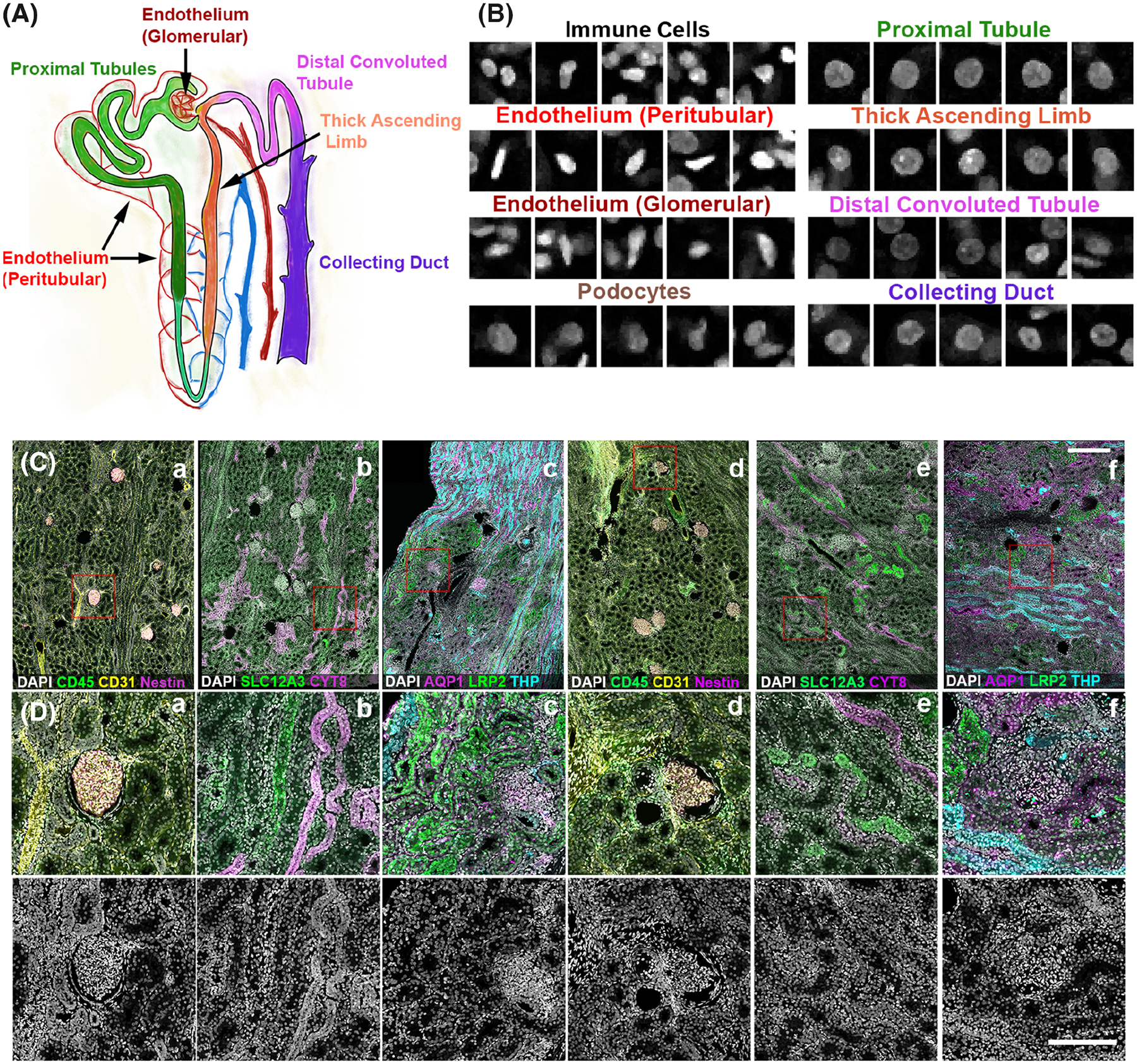
Uniqueness of nuclear morphology and staining signature of cell types found in the human kidney. A. Unique tubules and structures found in the nephron unit of the kidney. B. DAPI nuclear staining signature of various cell types identified manually based on specific markers (from C), location and morphology. C. 50 μm sections from human nephrectomy specimens were stained with three sets of markers all including DAPI in three different experiments. Tissue was imaged by tile scanning confocal microscopy and the images stitched together. D. Subregions from indicated red boxes in C. Bottom panels showing the DAPI channel only indicate the number and variety of nuclear morphology present in the cortex of the human kidney. Scale bars = 200 μm

3.2 |. Tissue Cytometry Using the Volumetric Tissue Exploration and Analysis (VTEA) Software Tool Can Be Used to Generate Large Amounts of Training Data with Cell Type Labels

VTEA cytometry tool was used to identify all cells based on a previously described nuclear segmentation and cytometry approach (13). Cell types were identified based on the fluorescence intensity of specific cell markers using an unsupervised machine learning clustering algorithm (Fig. 2). Visualization of the specific clusters in the image volume was also done using VTEA as an additional measure to validate the identity of cell types based on the expected spatial distribution and morphological characteristics in the tissue (Fig. 2). Image regions of interest were also used to limit specific localization dependent sub-populations, such as the endothelial cells in glomerulus vs peritubular space. VTEA supports projections and export of 3D volumes that can include surrounding signal or only the nuclei segmented by VTEA (Supporting Information Fig. S1, see Methods). Using this approach, ~230,000 cells were classified into eight different classes (Supporting Information Table S1). The corresponding 3D volumes, 3D volumes with context (Supporting Information Fig. S1B), 2D projections along the z-axis (z-projections), and 2D median z-axis slices were sorted and exported into “ground truth” libraries as NephNuc3D, NephNuc3D with context, NephNuc2D_Projection (without or with context), and NephNuc2D (without or with context), respectively (dataset available at the Broad Bioimaging Benchmark Collection, accession number BBBC051, https://bbbc.broadinstitute.org/BBBC051) (27).

FIG 2.

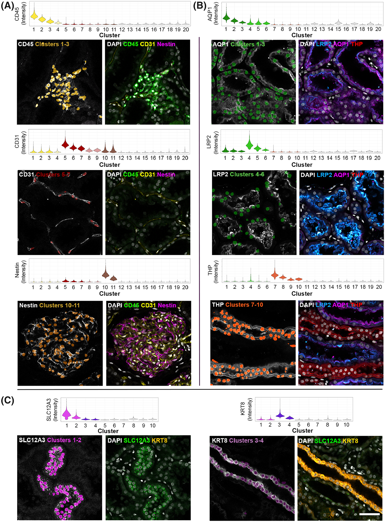
Training set generation and validation of cell type images. 50 μm sections from human nephrectomy specimens were stained with three sets of markers all including DAPI in three different experiments. Tissue was imaged by tile scanning confocal microscopy and images stitched together and processed for tissue cytometry by VTEA. Cells were classified by X-means clustering based on their associated marker intensity by unsupervised machine learning as outlined in the methods. Classified cells were mapped by cluster color on violin plots. Mapping of identified clusters is displayed on the left of each panel and original volumes at shown at the right. Tissue sections were stained with CD45, CD31 and Nestin (A), AQP1, LRP2, and THP (B) and SLC12A3 and KRT8 (C)

3.3 |. Using Classical Machine Learning and Shape-Based Descriptors for Classifying Cells Based on DAPI Nuclear Staining

To test if classical machine learning approaches could predict renal cell types based on the training data generated above by cytometry, image features were calculated on NephNuc3D data, NephNuc3D with context, and NephNuc2D_Projections without and with context datasets and used to train a Random Forest or support vector machine (SVM) classifier. The features calculated included pixel intensity statistics, Haralick texture features (28), parameter-free threshold adjacency statistics (29), spherical harmonics (30), and Zernike features (31). As multiple features could prove important to the predictive capacity of the classifiers, combinations of features were tested (32). The Random Forest classifier performed best when combining Haralick and PFTAS features (balanced accuracy 42.20%), nearly identical to using a SVM classifier (balanced accuracy 41.54%) or with the addition of image statistics (balanced accuracy 42.18%, Supporting Information Fig. S2, Table S2). Furthermore, a consistent improvement in balanced accuracy was observed between 2D and 3D images and with and without context. For instance, considering classification based on Haralick features and PFTAS the balanced accuracy increased from 36.05 to 38.05% for 2D images with and without context respectively and from 38.15 to 42.20% for 3D images with and without context, respectively (Supporting Information Table S2).

3.4 |. Convolutional Neural Network (CNN) Based Deep Learning Models Increase the Accuracy of Cell Classification

Next, a deep learning approach was tested to determine if we could improve the classification accuracy. For this, two convolutional neural networks were devised, NephNet2D and NephNet3D were devised to test the 2D or 3D training data, respectively. A third existing network was also finetuned with the 2D training data. The input for NephNet2D and ResNet-31 (33, 34) were NephNuc2D_Projection data or median z-axis slice 2D datasets. The input for NephNet3D was NephNuc3D or NephNuc3D with context. The architectures of NephNet2D and NephNet3D used are shown in Figure 3. Augmentation and hyperparameters selection settings are discussed in detail in the Methods section. The inclusion or exclusion of contextual, surrounding nuclei in the 2D or 3D data was examined to improve the accuracy.

FIG 3.

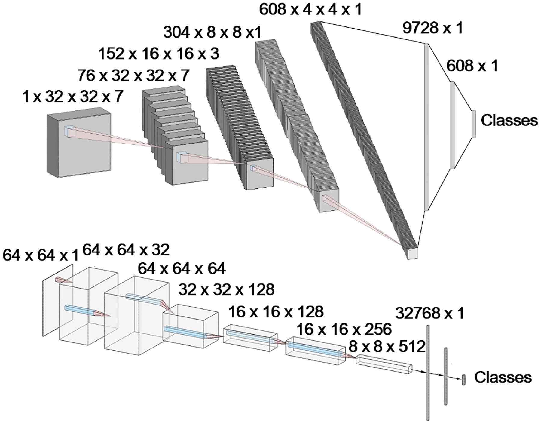
CNN Architectures for NephNet2D and NephNet3D. CNNs were developed and implemented in PyTorch. A. 2D CNN architecture, where each layer is separated by one 3 × 3 convolution, batch normalization, leaky ReLU, and max pooling with a stride of 2 × 2 × 2. Linear layers are separated by dropout normalization (P = 0.5). B. 3D architecture where each layer consisted of two 3 × 3 × 3 convolutions, batch normalization, leaky ReLU, and max pooling with a stride of 2 × 2 × 2. Linear layers are separated by dropout normalization (P = 0.5)

Both the dimension and content of the images affected the predictive ability of the CNNs. For the 2D slice, 2D maximum projections, and 3D volumes, adding the context surrounding the nuclei of interest improved the balanced accuracy (Fig. 4 and Supporting Information Table S2). The highest balanced accuracy was observed with NephNet3D trained with NephNuc3D with context, 80.26%, as compared to 66.55% and 60.82% with NephNet2D trained with NephNuc2D_Projection and NephNuc2D with context, respectively. Fivefold validation of NephNet3D trained with NephNuc3D with context gave a comparable mean balanced accuracy suggesting the model training or testing was not biased (79.01 ± 0.25%, Supporting Information Table S3). To understand the performance limits of NephNet3D trained with NephNuc3D with context images, low Softmax scored images (<0.45) were removed from the analysis, which culled 10.93 ± 0.54% of images and improved the balanced accuracy to 83.96 ± 1.04% (Supporting Information Table S3). Per class performance of NephNet3D trained with NephNuc3D with context images was calculated and the model made the most mistakes confusing distal convoluted tubule and collecting duct nuclei (distal convoluted tubule cell class F1-score = 0.58, Supporting Information Table S4 and Fig. 4B). Surprisingly, using the established and fine-tuned computer vision-trained network Resnet-31 CNN underperformed compared to NephNet2D (Supporting Information Fig. S3, Table S2).

FIG 4.

Cell classification based on nuclear staining using NephNet2D or NephNet3D and the NephNuc datasets. The NephNuc datasets were split into training and testing. The eight classes used for training are epithelial cells from the proximal tubules (PT), thick ascending limbs (TAL), distal convoluted tubules (DCT), and collecting duct (CD), and other cells such as leukocytes (Leuk), podocytes (Podo) and endothelial cells (Endo) in glomeruli (G) or in the peritubular (P) space. The testing datasets were classified, and accuracy and confusion matrices were generated. A. The balanced accuracies of networks trained on 2D sections (left) or 3D volumes (right) containing a single nucleus. B. The balanced accuracies of networks trained on 2D sections (left) or 3D (right) containing a nucleus and surrounding nuclei. Asterisks indicate specific weaknesses in either the 2D or 3D classifications and the influence of surrounding nuclei on the classification. In all configurations except 3D nuclei with surrounding nuclei, there were errors in classifying podocytes as leukocytes and glomerular endothelium (blue and green asterisks) and between epithelial cells (red asterisks). Surrounding nuclei, context, improved classification of DCT and CD (magenta asterisks, compare A to B)

The model with the highest balanced accuracy, NephNet3D trained on 3D image volumes with context, was subjected to noise and image resolution robustness testing to assess the effects of image quality on classification (Fig. 5). Down sampling the input images led to a rapid decrease in predictive performance. For example, a 2x down sample decreased the accuracy from 80.26% to 65.49%. The addition of noise at fixed levels mildly decreased the predictive performance, dropping from 80.26% to 77.45% at an α = 0.8 and 71.39% at an α = 0.6.

FIG 5.

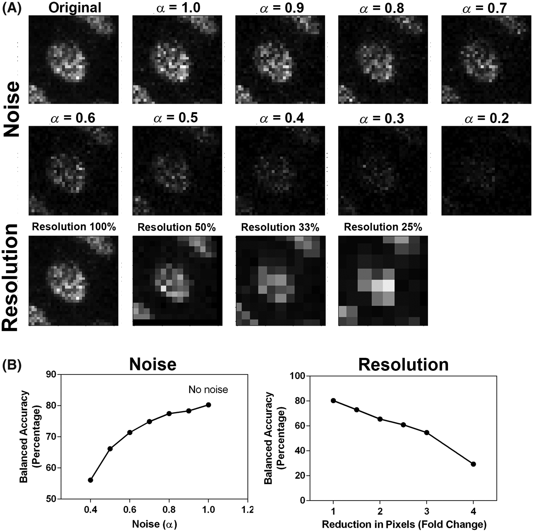
NephNet3D performance on noisy and lower resolution images. Increasing amounts of noise or decreasing resolution was used to generate testing datasets of 3D nuclei from the NephNuc3D with context data and classified with NephNet3D. A nearest neighbor approach was used for reducing the resolution of the image and noise was added by incorporating an α-factor described in the methods. A. Example of augmentation of training data with increasing noise or decreasing resolution for one nucleus. B. NephNet3D performance on testing data augmented by adding noise (left) or reducing the number of pixels to simulate less resolution (right)

3.5 |. Improving Classification in Novel specimens’ Accuracy by Subsampling

To improve the predictive ability of NephNet3D, multiple samples were included in the NephNuc datasets. As specimens from novel patients are analyzed, we expect there will be specimen-to-specimen variability. Thus, during training of NephNet3D, we tested if the ability to predict cell classification in a new specimen was improved by fine-tuning on fractions of that specimen. An early iteration of NephNet3D (trained only on Specimens 1 and 2, Supporting Information Table S1) was trained for 30 epochs on 1% of Specimen 3. This finetuning improved the balanced accuracy on the remaining nuclei of Specimen 3 from 58.3% to 74.2%. With 10% of Specimen 3 used for fine-tuning, the network’s balanced accuracy was 79.7%—nearly the same balanced accuracy of the fully trained NephNet3D network. When finetuning with more than 10% of Specimen 3, the balanced accuracy remained at 80%. This suggests that, if necessary, NephNet3D can be adapted to novel tissue with a small fraction of labeled nuclei (Fig. 6A).

FIG 6.

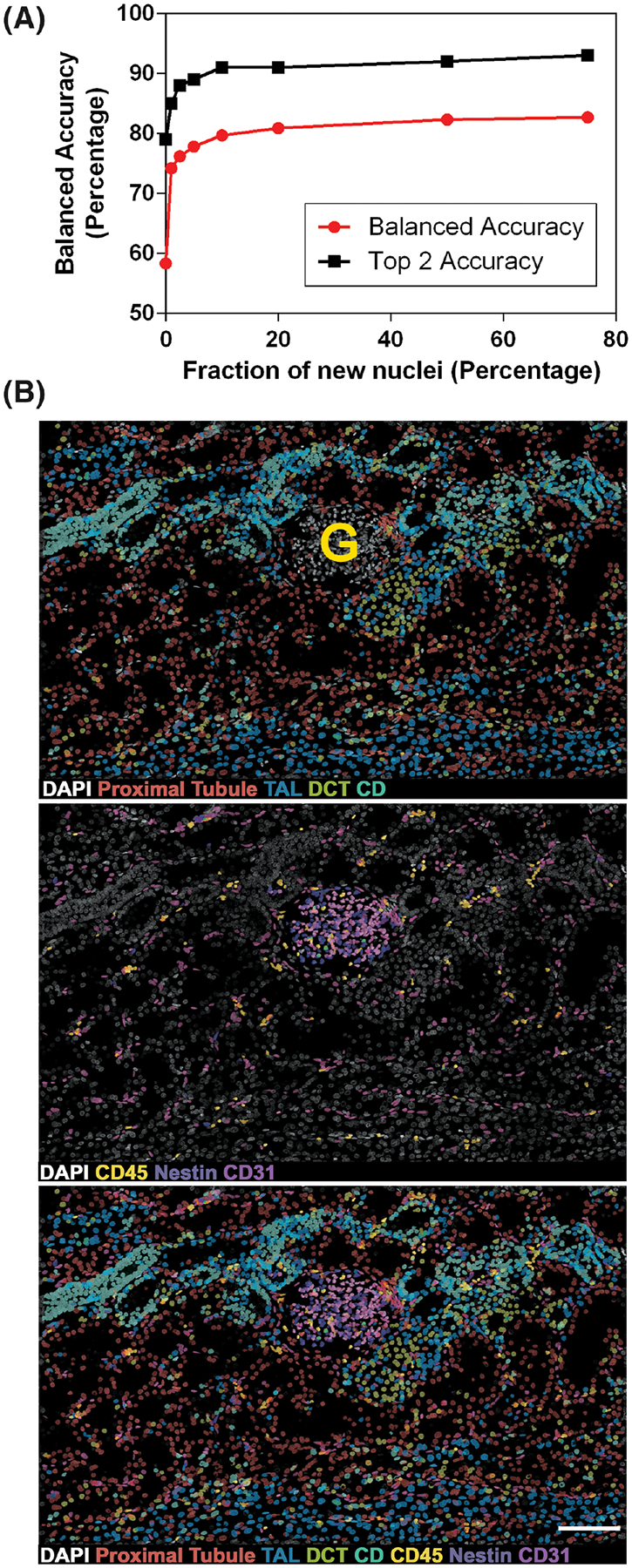
NephNet3D classification of cells in new image volumes. A. Finetuning of NephNet3D with nuclei from specimen 3 labeled for the eight cell types. 10% of Specimen 3 for fine tuning of NephNet3D trained on Specimens 1 and 2 is sufficient for near-peak balanced accuracy on the entire specimen. The CNN was fine-tuned on varying amounts of data from a new specimen (nephrectomy) prior to being tested on the nuclei from the new specimen. B. An image volume of DAPI stained nuclei not previously used, from Specimen 1, was segmented by VTEA and classified with NephNet3D. Overlay of predicted labels from NephNet3D on the DAPI stained nuclei. The overlays in the top panel are for cells classified as: Proximal tubules (red), TAL (blue), DCT (yellow-green) and CD (blue-green); in the middle panel, leukocytes (CD45, yellow), podocytes (Nestin, purple), and endothelium (CD31, magenta and pink). Bottom panel shows DAPI stained nuclei with all predicted labels. G indicates a glomerulus. One hundred and seventy-seven segmented object/nuclei were manually classified by an expert. NephNet3D had an agreement of 67.9% (balanced accuracy as compared to expert classified nuclei). Maximum Z-projections are shown, scale bar = 100 μm

3.6 |. Improving Classification by Training Data Augmentation

Supervised classification generally performs better if the training data have sufficient variability. This is particularly true for deep learning-based classification, as such models have very large number of parameters, which require sufficient variability in the training data to avoid overfitting. Furthermore, unlike natural images, which often have a horizon, the orientation and rotation of a nucleus in the image is variable. To overcome this problem, data augmentation is used during training to increase data variability and mitigate the overfitting issue. The image augmentation steps we considered included transformation, rotation, flip, and noise injection (Supporting Information Fig. S4). The balanced accuracy on training without augmentation was 13%, 45%, and 53% for 2D model, 3D model without context, and 3D model with context, respectively. In contrast, training using augmented training data yielded a balanced accuracy of 29%, 53%, and 80% for 2D model, 3D model without context, and 3D model with context data, respectively.

3.7 |. NephNet3D with VTEA Tissue Cytometry Can Classify and Spatially Map Cell Types in Image Volumes Stained Only with DAPI

The goal of this methodology is to classify cell types in image volumes based only on the DAPI nuclear staining. To establish feasibility, a new image volume of a kidney cortical section stained with DAPI that was not used in previous training and from the same specimen cohort was tested. Image volumes of all the nuclei were generated by VTEA and then processed by the trained NephNet3D to predict the classes of the cells. Classified nuclei were visualized on the image volume using VTEA, which allowed a “pseudo” highlighting of cells (Fig. 6B). These predictions by NephNet3D were compared to classification by an expert (using nuclear shape and spatial cues) on a subsample of the image volume. Across all eight classes, NephNet3D had a balanced accuracy of 67.9% as compared to an expert’s classification. The NephNet3D and expert classifications showed fair agreement with a Kappa statistic of 0.35. Furthermore, upon examining the cell classifications mapped back to the image volume, cells classified as epithelial cells outlined contiguous tubular structures (Fig. 6B, top panel) while cells classified as endothelial or immune cells were confined to either the interstitium or glomeruli (Fig. 6B, middle panel). Strikingly, cells classified as podocytes were almost exclusively confined to the single glomerulus in the image volume (Fig. 6B).

4 |. DISCUSSION

In this work, we devised an approach to classify cells in situ within intact kidney tissue, using an imaging-based approach that relies on nuclear staining. To accomplish this goal, we used tissue cytometry to efficiently generate a large amount of training data, consisting of image volumes of nuclei classified based on their association with specific cell markers within the human kidney. This dataset was used to determine the optimal machine learning approach that could provide the highest classification accuracy based on this nuclear staining. Our results show that a deep learning approach outperforms traditional supervised classification methods, and that a CNN trained on 3D image volumes with context (with nearby nuclei) provides the highest balanced accuracy. The utility of this classification pipeline was demonstrated on an unexplored kidney tissue whereby cells were successfully classified into eight types and visualized based only on 3D nuclear staining.

Image-based classification of cells has several applications in biology and medicine (9). Some commonly recognized applications are in drug screening and discovery (21, 35), genetic screening (36), cell biology (37), and digital pathology (10). These last two applications are commonly used in the context of cell classification in intact tissue. Cell biology applications include cell classification based on nuclear and other specific markers or spatial analyzes, similar to what we and others described as tissue cytometry using fluorescence or histochemical markers (12, 13, 18, 38, 39). Many efforts are also focused on cell segmentation, automated detection and counting (40). Digital pathology relies on histology staining and has experienced exciting development in cell segmentation and classification (8, 41–43). Several approaches have been described to classify cells based only on nuclear staining in digital pathology images, such as standard machine learning classifiers, numerical feature engineering, neural networks, and transport-based morphometry (9, 10, 22). However, many of these approaches are focused on cancer detection or identification of unique cell phenotypes (10, 11). An approach that can allow non-exhaustive cell classification in tissue based only on 3D nuclear signature has not been previously described.

Our approach performs well when compared to state-of-the-art methods across imaging modalities. For comparison, we considered classification of images of unstained cells, histology stained tissue and fluorescently labeled nuclei: (1) the classification of mitotic state by brightfield images from imaging flow cytometry with DeepFlow, an imbalanced five or seven class problem, had a balanced accuracy of 58 or 60% respectively (23, 44), (2) classification of seven classes of cells in histology images with HoVer-Net had per class F1-scores of 0.4 to 0.6 (45), (3) classification of five classes of leukocytes in histology images with WBCsNET had a balanced accuracy of 91% (46), (4) classification of four classes of immune cells in histology images had an overall accuracy of 97% by multiple models (47), and (5) classification of mitotic state (G2 vs G1/S, only two classes) with images of fluorescently labeled nuclei, had an accuracy of 85–90% (48) (Supporting Information Table S5). If we compare to the multiclass models with seven classes, DeepFlow and HoVer-Net, our 3D-CNN model performs better with more classes (eight total classes, with a balanced accuracy of 80.26% and per class F1-scores of 0.5 to 0.8). Although, our model’s performance could improve to match accuracies seen with models trained on fewer classes (e.g., WBCsNet), this summary shows our model is on-par and in some cases better than state-of-the-art approaches for more than five classes. Furthermore, our approach is unique amongst these multiclass cell classification models as it can be incorporated with highly multiplexed immunofluorescence imaging techniques (e.g., CODEX, CycIF, MxIF, etc.) (14, 16, 49).

A strength of our approach is that it uniquely combines tissue cytometry and deep learning to classify cells based on their 3D nuclear staining in intact tissues. Tissue cytometry using VTEA is essential to generate the training dataset and visualize the classified cell in situ. Generating training data is arguably one of the most arduous tasks in any machine learning approach. VTEA allowed us to generate 230,000 labeled nuclei quickly in a matter of weeks. Furthermore, VTEA will keep track of the nuclei and map them to the tissue for visualization after classification, allowing their classification to be interpreted in the setting of their spatial distribution and relationship to other cells and structures. In the kidney, this is critical in interpreting how specific cell types are linked to biological function or dys-function, and we envision that this will also be important when applied to other organs.

The approach proposed in this work will likely have important applications in the setting of sparse tissue. The described workflow enables continued re-evaluation of existing imaging data, thereby reducing the need for additional tissue. Indeed, as new cell markers emerge, the deep learning approach can be trained to recognize these new nuclear signatures in ground truth datasets generated in an abundant source of tissue, such as the specimen used in this study. New classifications or sub-classifications can then be imputed on existing datasets from sparse tissue without the need for additional sectioning and depletion of the tissue. This is especially useful in the setting of a kidney biopsy, which is a needle biopsy with a small amount of tissue (19, 50). DAPI staining can be easily incorporated with other technologies. For example, our approach can be extended to specimen prepared for RNA exploration, and cell classification can become highly integrated by incorporating signatures from various levels of gene expression (51). Although this overall approach has been tailored to the complexity of kidney tissue, it can be applied to other organs. Furthermore, the model of continuous data extraction from a single archived dataset may facilitate data sharing and collaboration.

Comparing the different approaches and networks supports the conclusion that a 3D CNN architecture was best at predicting cell class based on nuclear staining and showed marked improvement over a 2D architecture tested with various types of data. The 3D CNN, with 3D data, was particularly important for improving the classification accuracy of cells within the glomerulus and proximal tubules. Furthermore, NephNet3D showed increased accuracy for the podocyte, proximal tubule, thick ascending limb, collecting duct, and glomerular endothelium cell classes. This improvement supports the idea that important features are contained within the three-dimensional structure of the nucleus for each cell type. Importantly, NephNet3D did have trouble classifying or discriminating between tubular epithelium of adjacent segments, such as the collecting duct and distal tubule. This could be due to the biological reliability of the cell markers, the variability in expression of the markers (e.g., Sample 3, Supporting Information Table S1) or overlap in transition areas, biological similarity, between tubular segments (25). In fact, the poor predictive capacity in these transitional regions (e.g. DCT to CD) could be used as a method to identify transitional cells or possibly novel subtypes of the tubular epithelium.

The wide availability of 2D imaging modalities, clinically and in research, argues for developing 2D approaches for cellular classification. We demonstrate fair performance (~60% balanced accuracy) of a 2D architecture. We also demonstrate poor performance (~30% balanced accuracy), worse than our 2D approach, of a pretrained network, Resnet-31 (33). Thus, our 2D network could be a better starting point for additional refinement of a 2D approach. Furthermore, our work demonstrates the importance of data collection at an appropriate resolution and signal/noise for the predictive ability of deep learning using nuclear information. This may provide a guide for future data collection on additional imaging modalities more common in 2D imaging, including slide-scanners and other high-content platforms. Importantly, we expect both our 2D and 3D architectures will be refined through additional data collection to establish more classes of nuclei, more depth within classes and to cover other imaging platforms and modalities. Our network and data are publicly available to the community for such development.

Our study has several limitations. The approach used is specialized and may not be broadly applicable because of the need for expertise in imaging and computer science as well as the need for high performance computing hardware. Despite having a training dataset of thousands of curated nuclear volumes, we anticipate that the training dataset will need to expand significantly for the accuracy to improve. Since the dataset has been generated from just three tissue samples, expanding the dataset with additional specimens will further improve the generalizability of this approach. Also, the resolution at which the data was collected, and subsequent quality of segmentation, may place SPHARM or numerical feature-based approaches at a disadvantage a priori, because these approaches may require a higher resolution image to be most effective. However, balancing feasibility and the economy of time/resource constraints, the current data acquisition settings are commonly used (17). Therefore, it is reasonable to assert that for standard large-scale 3D image acquisition, NephNet3D is likely the most optimal approach for cell classification based on nuclear staining.

The deep-learning multi-class classification approach proposed here will augment on-going advancements in the spatial transcriptomics. Like single cell sequencing, spatial transcriptomics is proving to be a disruptive technology. Spatial transcriptomics can be divided between fluorescence in situ hybridization (FISH) based (e.g., merFISH, seqFISH, etc.) (52–57) and bead arrays based with sequencing (e.g., Visium, Silde-Seq) (58). Bead array approaches have nearly cellular resolution and often include a registration image of the sample with a histology stain to understand the transcriptomics in the structural context of the tissue. Likewise, a nuclei image could be collected for classification by our proposed deep learning approach. In contrast, FISH approaches can have the transcriptomic depth and are spatially resolved-often requiring diffraction limited imaging. Thus, FISH can be a long and expensive experiments to perform due to required higher resolution imaging for longer imaging times and, in some cases, thousands of probes. Because FISH approaches are often compatible with standard immunofluorescence and small-molecule stains such as DAPI, our classification strategy could also be included to shorten the imaging time and lessen the cost as panels of probes may not be necessary. Thus, our classification approach is complementary to spatial transcriptomics.

The current work was done on reference tissue from donor nephrectomy specimens. Kidney disease will likely alter the nuclear staining signature of cells because of metabolic stress or cellular injury (59), thereby potentially changing the classification of some cells or presenting a new subclass for a particular cell type (23). Investigating these changes and distribution at the tissue level will likely aid in understanding the pathophysiology of the disease, especially in early stages where such subtle cellular changes may precede obvious structural abnormalities. We propose that the cytometry approach will facilitate this process. The visualization feature of VTEA can map all cell types, including diseased cell populations. By comparing localization and changes to reference tissue, diseased cells can be reclassified and could serve as ground truth for a disease subclassification. Such iterative learning models are subject of ongoing and future investigations in our lab. In addition, since we showed that only a small fraction of appropriately classified nuclei from a tissue is enough to maximize the accuracy of cell class prediction for that particular tissue, expanding our training dataset to new subclasses of cells may conform with our goals of tissue economy, even when only sparse tissue is available for ground truth generation.

Our work here does not address which specific features in the nuclei are key determinants of their classification. The explainability and human readability of the deep learning approaches are still at an early stage (60). However, since the signatures of nuclear staining are linked to chromatin condensation and cellular activity (20, 23), it is possible that our work could present an opportunity to recognize the salient features in nuclei that dictate their classification. For this, we plan to use class saliency map and attribution-based approaches to understand the specific image features which impacted the classification decision made by the deep learning models. This is a subject of ongoing research.

In conclusion, by combining tissue cytometry and a deep learning CNN, we present an approach for in situ classification of cell types in the human kidney using 3D nuclear staining. This classification methodology allows the preservation of tissue architecture and spatial context of each cell and has potential advantages on tissue economy and non-exhaustive analysis of existing data.

REFERENCES

- 1.Nawata CM, Pannabecker TL. Mammalian urine concentration: A review of renal medullary architecture and membrane transporters. J Comp Physiol B 2018;188:899–918. [DOI] [PMC free article] [PubMed] [Google Scholar]
- 2.Park J, Shrestha R, Qiu C, Kondo A, Huang S, Werth M, Li M, Barasch J, Suszták K. Single-cell transcriptomics of the mouse kidney reveals potential cellular targets of kidney disease. Science 2018;360: 758–763. [DOI] [PMC free article] [PubMed] [Google Scholar]
- 3.Stewart BJ, Ferdinand JR, Young MD, Mitchell TJ, Loudon KW, Riding AM, Richoz N, Frazer GL, Staniforth JUL, Vieira Braga FA, et al. Spatiotemporal immune zonation of the human kidney. Science 2019; 365:1461–1466. [DOI] [PMC free article] [PubMed] [Google Scholar]
- 4.Taal MW, Brenner BM, Rector FC. Brenner and Rector’s the Kidney. 9th ed. Philadelphia: Elsevier/Saunders, 2012. [Google Scholar]
- 5.Lake BB, Chen S, Hoshi M, Plongthongkum N, Salamon D, Knoten A, Vijayan A, Venkatesh R, Kim EH, Gao D, et al. A single-nucleus RNA-sequencing pipeline to decipher the molecular anatomy and pathophysiology of human kidneys. Nat Commun 2019;10:2832. [DOI] [PMC free article] [PubMed] [Google Scholar]
- 6.Wilson PC, Wu H, Kirita Y, Uchimura K, Ledru N, Rennke HG, Welling PA, Waikar SS, Humphreys BD. The single-cell transcriptomic landscape of early human diabetic nephropathy. Proc Natl Acad Sci U S A 2019;116:19619–19625. [DOI] [PMC free article] [PubMed] [Google Scholar]
- 7.Menon R, Otto EA, Hoover P, Eddy S, Mariani L, Godfrey B, Berthier CC, Eichinger F, Subramanian L, Harder J, et al. Single cell transcriptomics identifies focal segmental glomerulosclerosis remission endothelial biomarker. JCI Insight 2020;5:e133267. 10.1172/jci.insight.133267. [DOI] [PMC free article] [PubMed] [Google Scholar]
- 8.Madabhushi A, Lee G. Image analysis and machine learning in digital pathology: Challenges and opportunities. Med Image Anal 2016;33: 170–175. [DOI] [PMC free article] [PubMed] [Google Scholar]
- 9.Shifat ERM, Yin X, Fitzgerald CE, Rohde GK. Cell image classification: A comparative overview. Cytometry Part A 2020;97A:347–362. [DOI] [PubMed] [Google Scholar]
- 10.Janowczyk A, Madabhushi A. Deep learning for digital pathology image analysis: A comprehensive tutorial with selected use cases. J Pathol Inform 2016;7:29. [DOI] [PMC free article] [PubMed] [Google Scholar]
- 11.Qi Q, Li Y, Wang J, Zheng H, Huang Y, Ding X, Rohde GK. Label-efficient breast cancer histopathological image classification. IEEE J Biomed Health Inform 2019;23:2108–2116. [DOI] [PubMed] [Google Scholar]
- 12.Gerner MY, Kastenmuller W, Ifrim I, Kabat J, Germain RN. Histo-cytometry: A method for highly multiplex quantitative tissue imaging analysis applied to dendritic cell subset microanatomy in lymph nodes. Immunity 2012;37:364–376. [DOI] [PMC free article] [PubMed] [Google Scholar]
- 13.Winfree S, Khan S, Micanovic R, Eadon MT, Kelly KJ, Sutton TA, Phillips CL, Dunn KW, el-Achkar TM. Quantitative three-dimensional tissue cytometry to study kidney tissue and resident immune cells. J Am Soc Nephrol 2017;28:2108–2118. [DOI] [PMC free article] [PubMed] [Google Scholar]
- 14.Goltsev Y, Samusik N, Kennedy-Darling J, Bhate S, Hale M, Vazquez G, Black S, Nolan GP. Deep profiling of mouse splenic architecture with CODEX multiplexed imaging. Cell 2018;174: 968–981. e15. [DOI] [PMC free article] [PubMed] [Google Scholar]
- 15.Berens ME, Sood A, Barnholtz-Sloan JS, Graf JF, Cho S, Kim S, Kiefer J, Byron SA, Halperin RF, Nasser S, et al. Multiscale, multimodal analysis of tumor heterogeneity in IDH1 mutant vs wild-type diffuse gliomas. PLoS One 2019;14:e0219724. [DOI] [PMC free article] [PubMed] [Google Scholar]
- 16.Lin JR, Izar B, Wang S, Yapp C, Mei S, Shah PM, Santagata S, Sorger PK. Highly multiplexed immunofluorescence imaging of human tissues and tumors using t-CyCIF and conventional optical microscopes. Elife 2018;7. 10.7554/eLife.31657.001. [DOI] [PMC free article] [PubMed] [Google Scholar]
- 17.Winfree S, Ferkowicz MJ, Dagher PC, Kelly KJ, Eadon MT, Sutton TA, Markel TA, Yoder MC, Dunn KW, el-Achkar TM. Large-scale 3-dimensional quantitative imaging of tissues: State-of-the-art and translational implications. Transl Res 2017;189:1–12. [DOI] [PMC free article] [PubMed] [Google Scholar]
- 18.Stoltzfus CR, Filipek J, Gern BH, Olin BE, Leal JM, Wu Y, Lyons-Cohen MR, Huang JY, Paz-Stoltzfus CL, Plumlee CR, et al. CytoMAP: A spatial analysis toolbox reveals features of myeloid cell organization in lymphoid tissues. Cell Rep 2020;31:107523. [DOI] [PMC free article] [PubMed] [Google Scholar]
- 19.Winfree S, Dagher PC, Dunn KW, Eadon MT, Ferkowicz M, Barwinska D, Kelly KJ, Sutton TA, el-Achkar TM. Quantitative large-scale three-dimensional imaging of human kidney biopsies: A bridge to precision medicine in kidney disease. Nephron 2018;140:134–139. [DOI] [PMC free article] [PubMed] [Google Scholar]
- 20.Kapuscinski J DAPI: a DNA-specific fluorescent probe. Biotech Histochem 1995;70:220–233. [DOI] [PubMed] [Google Scholar]
- 21.Carpenter AE, Jones TR, Lamprecht MR, Clarke C, Kang IH, Friman O, Guertin DA, Chang J, Lindquist RA, Moffat J, et al. CellProfiler: Image analysis software for identifying and quantifying cell phenotypes. Genome Biol 2006;7:R100. [DOI] [PMC free article] [PubMed] [Google Scholar]
- 22.Basu S, Kolouri S, Rohde GK. Detecting and visualizing cell phenotype differences from microscopy images using transport-based morphometry. Proc Natl Acad Sci U S A 2014;111:3448–3453. [DOI] [PMC free article] [PubMed] [Google Scholar]
- 23.Eulenberg P, Kohler N, Blasi T, Filby A, Carpenter AE, Rees P, Theis FJ, Wolf FA. Reconstructing cell cycle and disease progression using deep learning. Nat Commun 2017;8(1):463. 10.1038/s41467-017-00623-3. [DOI] [PMC free article] [PubMed] [Google Scholar]
- 24.Tone S, Sugimoto K, Tanda K, Suda T, Uehira K, Kanouchi H, Samejima K, Minatogawa Y, Earnshaw WC. Three distinct stages of apoptotic nuclear condensation revealed by time-lapse imaging, biochemical and electron microscopy analysis of cell-free apoptosis. Exp Cell Res 2007;313:3635–3644. [DOI] [PMC free article] [PubMed] [Google Scholar]
- 25.Lee JW, Chou CL, Knepper MA. Deep sequencing in microdissected renal tubules identifies nephron segment-specific transcriptomes. J Am Soc Nephrol 2015;26:2669–2677. [DOI] [PMC free article] [PubMed] [Google Scholar]
- 26.Thul PJ, Lindskog C. The human protein atlas: A spatial map of the human proteome. Protein Sci 2018;27:233–244. [DOI] [PMC free article] [PubMed] [Google Scholar]
- 27.Ljosa V, Sokolnicki KL, Carpenter AE. Annotated high-throughput microscopy image sets for validation. Nat Methods 2012;9:637. [DOI] [PMC free article] [PubMed] [Google Scholar]
- 28.Haralick RM. Statistical and structural approaches to texture. Proc IEEE 1979;67:786–804. [Google Scholar]
- 29.Hamilton NA, Pantelic RS, Hanson K, Teasdale RD. Fast automated cell phenotype image classification. BMC Bioinformatics 2007;8:110. [DOI] [PMC free article] [PubMed] [Google Scholar]
- 30.Medyukhina A, Blickensdorf M, Cseresnyes Z, Ruef N, Stein JV, Figge MT. Dynamic spherical harmonics approach for shape classification of migrating cells. Sci Rep 2020;10:6072. [DOI] [PMC free article] [PubMed] [Google Scholar]
- 31.Boland MV, Markey MK, Murphy RF. Automated recognition of patterns characteristic of subcellular structures in fluorescence microscopy images. Cytometry 1998;33:366–375. [PubMed] [Google Scholar]
- 32.Caicedo JC, Cooper S, Heigwer F, Warchal S, Qiu P, Molnar C, Vasilevich AS, Barry JD, Bansal HS, Kraus O, et al. Data-analysis strategies for image-based cell profiling. Nat Methods 2017;14: 849–863. [DOI] [PMC free article] [PubMed] [Google Scholar]
- 33.Habibzadeh M, Jannesari M, Rezaei Z, Baharvand H, Totonchi M. Automatic white blood cell classification using pre-trained deep learning models: ResNet and Inception: SPIE; 2018.
- 34.Ioannidou A, Chatzilari E, Nikolopoulos S, Kompatsiaris I. 3D ResNets for 3D Object Classification, In Kompatsiaris I, Huet B, Mezaris V, Gurrin C, Cheng W-H, Vrochidis S (Eds.), MultiMedia Modeling 25th International Conference, MMM 2019, Thessaloniki, Greece, January 8–11, 2019, Proceedings, Part I. p. 495–506. [Google Scholar]
- 35.Loo LH, Wu LF, Altschuler SJ. Image-based multivariate profiling of drug responses from single cells. Nat Methods 2007;4:445–453. [DOI] [PubMed] [Google Scholar]
- 36.Conrad C, Gerlich DW. Automated microscopy for high-content RNAi screening. J Cell Biol 2010;188:453–461. [DOI] [PMC free article] [PubMed] [Google Scholar]
- 37.Chen Y, Ladi E, Herzmark P, Robey E, Roysam B. Automated 5-D analysis of cell migration and interaction in the thymic cortex from time-lapse sequences of 3-D multi-channel multi-photon images. J Immunol Methods 2009;340:65–80. [DOI] [PMC free article] [PubMed] [Google Scholar]
- 38.Riordan DP, Varma S, West RB, Brown PO. Automated analysis and classification of histological tissue features by multi-dimensional microscopic molecular profiling. PLoS One 2015;10:e0128975. [DOI] [PMC free article] [PubMed] [Google Scholar]
- 39.Bjornsson CS, Lin G, Al-Kofahi Y, Narayanaswamy A, Smith KL, Shain W, Roysam B. Associative image analysis: A method for automated quantification of 3D multi-parameter images of brain tissue. J Neurosci Methods 2008;170:165–178. [DOI] [PMC free article] [PubMed] [Google Scholar]
- 40.Dunn KW, Fu C, Ho DJ, Lee S, Han S, Salama P, Delp EJ. DeepSynth: Three-dimensional nuclear segmentation of biological images using neural networks trained with synthetic data. Sci Rep 2019;9:18295. [DOI] [PMC free article] [PubMed] [Google Scholar]
- 41.Janowczyk A, Doyle S, Gilmore H, Madabhushi A. A resolution adaptive deep hierarchical (RADHicaL) learning scheme applied to nuclear segmentation of digital pathology images. Comput Methods Biomech Biomed Eng Imaging Vis 2018;6:270–276. [DOI] [PMC free article] [PubMed] [Google Scholar]
- 42.Kumar N, Verma R, Sharma S, Bhargava S, Vahadane A, Sethi A. A dataset and a technique for generalized nuclear segmentation for computational pathology. IEEE Trans Med Imaging 2017;36: 1550–1560. [DOI] [PubMed] [Google Scholar]
- 43.Rohde GK. New methods for quantifying and visualizing information from images of cells: An overview. Conf Proc IEEE Eng Med Biol Soc 2013;2013:121–124. [DOI] [PMC free article] [PubMed] [Google Scholar]
- 44.Lippeveld M, Knill C, Ladlow E, Fuller A, Michaelis LJ, Saeys Y, Filby A, Peralta D. Classification of human white blood cells using machine learning for stain-free imaging flow cytometry. Cytometry A 2020;97:308–319. [DOI] [PubMed] [Google Scholar]
- 45.Graham S, Vu QD, Raza SEA, Azam A, Tsang YW, Kwak JT, Rajpoot N. Hover-net: Simultaneous segmentation and classification of nuclei in multi-tissue histology images. Med Image Anal 2019;58: 101563. [DOI] [PubMed] [Google Scholar]
- 46.Shahin AI, Guo Y, Amin KM, Sharawi AA. White blood cells identification system based on convolutional deep neural learning networks. Comput Methods Programs Biomed 2019;168:69–80. [DOI] [PubMed] [Google Scholar]
- 47.Kutlu H, Avci E, Ozyurt F. White blood cells detection and classification based on regional convolutional neural networks. Med Hypotheses 2020;135:109472. [DOI] [PubMed] [Google Scholar]
- 48.Nagao Y, Sakamoto M, Chinen T, Okada Y, Takao D. Robust classification of cell cycle phase and biological feature extraction by image-based deep learning. Mol Biol Cell 2020;31:1346–1354. [DOI] [PMC free article] [PubMed] [Google Scholar]
- 49.Gerdes MJ, Sevinsky CJ, Sood A, Adak S, Bello MO, Bordwell A, Can A, Corwin A, Dinn S, Filkins RJ, et al. Highly multiplexed single-cell analysis of formalin-fixed, paraffin-embedded cancer tissue. Proc Natl Acad Sci U S A 2013;110:11982–11987. [DOI] [PMC free article] [PubMed] [Google Scholar]
- 50.Mai J, Yong J, Dixson H, Makris A, Aravindan A, Suranyi MG, Wong J. Is bigger better? A retrospective analysis of native renal biopsies with 16 gauge versus 18 gauge automatic needles. Nephrology (Carlton) 2013;18:525–530. [DOI] [PubMed] [Google Scholar]
- 51.Shah S, Takei Y, Zhou W, Lubeck E, Yun J, Eng CL, Koulena N, Cronin C, Karp C, Liaw EJ. Dynamics and spatial genomics of the nascent transcriptome by intron seqFISH. Cell 2018;174: 363–376. e16. [DOI] [PMC free article] [PubMed] [Google Scholar]
- 52.Moffitt JR, Hao J, Bambah-Mukku D, Lu T, Dulac C, Zhuang X. High-performance multiplexed fluorescence in situ hybridization in culture and tissue with matrix imprinting and clearing. Proc Natl Acad Sci U S A 2016;113:14456–14461. [DOI] [PMC free article] [PubMed] [Google Scholar]
- 53.Moffitt JR, Hao J, Wang G, Chen KH, Babcock HP, Zhuang X. High-throughput single-cell gene-expression profiling with multiplexed error-robust fluorescence in situ hybridization. Proc Natl Acad Sci U S A 2016;113:11046–11051. [DOI] [PMC free article] [PubMed] [Google Scholar]
- 54.Moffitt JR, Zhuang X. RNA imaging with multiplexed error-robust fluorescence in situ hybridization (MERFISH). Methods Enzymol 2016;572:1–49. [DOI] [PMC free article] [PubMed] [Google Scholar]
- 55.Eng CL, Lawson M, Zhu Q, Dries R, Koulena N, Takei Y, Yun J. Transcriptome-scale super-resolved imaging in tissues by RNA seqFISH. Nature 2019;568:235–239. [DOI] [PMC free article] [PubMed] [Google Scholar]
- 56.Shah S, Lubeck E, Zhou W, Cai L. seqFISH accurately detects transcripts in single cells and reveals robust spatial organization in the hippocampus. Neuron 2017;94:752–758. e1. [DOI] [PubMed] [Google Scholar]
- 57.Shah S, Lubeck E, Zhou W, Cai L. In situ transcription profiling of single cells reveals spatial organization of cells in the mouse hippocampus. Neuron 2016;92:342–357. [DOI] [PMC free article] [PubMed] [Google Scholar]
- 58.Rodriques SG, Stickels RR, Goeva A, Martin CA, Murray E, Vanderburg CR, Welch J, Chen LM, Chen F, Macosko EZ. Slide-seq: A scalable technology for measuring genome-wide expression at high spatial resolution. Science 2019;363:1463–1467. [DOI] [PMC free article] [PubMed] [Google Scholar]
- 59.Reidy K, Kang HM, Hostetter T, Susztak K. Molecular mechanisms of diabetic kidney disease. J Clin Invest 2014;124:2333–2340. [DOI] [PMC free article] [PubMed] [Google Scholar]
- 60.Holzinger A, Langs G, Denk H, Zatloukal K, Muller H. Causability and explainability of artificial intelligence in medicine. Wiley Interdiscip Rev Data Min Knowl Discov 2019;9:e1312. [DOI] [PMC free article] [PubMed] [Google Scholar]
- 61.Schindelin J, Arganda-Carreras I, Frise E, Kaynig V, Longair M, Pietzsch T, Preibisch S, Rueden C, Saalfeld S, Schmid B, et al. Fiji: An open-source platform for biological-image analysis. Nat Methods 2012;9:676–682. [DOI] [PMC free article] [PubMed] [Google Scholar]
- 62.Pedregosa F, Varoquaux G, Gramfort A, Michel V, Thirion B, Grisel O, Blondel M, Prettenhofer P, Weiss R, Dubourg V. Scikit-learn: Machine learning in python. Journal of Machine Learning Research 2011;12(85): 2825–2830. [Google Scholar]
- 63.He K, Zhang X, Ren S, Sun J. Deep residual learning for image recognition. arXiv 2015; 1512.03385.https://arxiv.org/abs/1512.03385. [Google Scholar]
- 64.Li L, Jamieson K, DeSalvo G, Rostamizadeh A, Talwalkar A. Hyper-band: A novel bandit-based approach to hyperparameter optimization. J Mach Learn Res 2017;18:6765–6816. [Google Scholar]
- 65.Paszke A, Gross S, Massa F, Lerer A, Bradbury J, Chanan G, et al. PyTorch: An Imperative Style, High-Performance Deep Learning Library. In Wallach H, Larochelle H, Beygelzimer A, Fox F,E, & Garnett R (Eds.), Advances in Neural Information Processing Systems 32. Curran Associates, Inc.; 2019. pp. 8024–8035. Available at: http://papers.neurips.cc/paper/9015-pytorch-an-imperative-style-high-performance-deep-learning-library.pdf [Google Scholar]
Associated Data
This section collects any data citations, data availability statements, or supplementary materials included in this article.