Dermatologist–level classification of skin cancer with deep neural networks

Abstract

Skin cancer, the most common human malignancy^1–3, is primarily diagnosed visually, beginning with an initial clinical screening and followed potentially by dermoscopic analysis, a biopsy and histopathological examination. Automated classification of skin lesions using images is a challenging task owing to the fine-grained variability in the appearance of skin lesions. Deep convolutional neural networks (CNNs)^4,5 show potential for general and highly variable tasks across many fine-grained object categories^6–11. Here we demonstrate classification of skin lesions using a single CNN, trained end-to-end from images directly, using only pixels and disease labels as inputs. We train a CNN using a dataset of 129,450 clinical images—two orders of magnitude larger than previous datasets¹²—consisting of 2,032 different diseases. We test its performance against 21 board-certified dermatologists on biopsy-proven clinical images with two critical binary classification use cases: keratinocyte carcinomas versus benign seborrheic keratoses; and malignant melanomas versus benign nevi. The first case represents the identification of the most common cancers, the second represents the identification of the deadliest skin cancer. The CNN achieves performance on par with all tested experts across both tasks, demonstrating an artificial intelligence capable of classifying skin cancer with a level of competence comparable to dermatologists. Outfitted with deep neural networks, mobile devices can potentially extend the reach of dermatologists outside of the clinic. It is projected that 6.3 billion smartphone subscriptions will exist by the year 2021 (ref. 13) and can therefore potentially provide low-cost universal access to vital diagnostic care.

There are 5.4 million new cases of skin cancer in the United States² every year. One in five Americans will be diagnosed with a cutaneous malignancy in their lifetime. Although melanomas represent fewer than 5% of all skin cancers in the United States, they account for approximately 75% of all skin-cancer-related deaths, and are responsible for over 10,000 deaths annually in the United States alone. Early detection is critical, as the estimated 5-year survival rate for melanoma drops from over 99% if detected in its earliest stages to about 14% if detected in its latest stages. We developed a computational method which may allow medical practitioners and patients to proactively track skin lesions and detect cancer earlier. By creating a novel disease taxonomy, and a disease-partitioning algorithm that maps individual diseases into training classes, we are able to build a deep learning system for automated dermatology.

Previous work in dermatological computer-aided classification^12,14,15 has lacked the generalization capability of medical practitioners owing to insufficient data and a focus on standardized tasks such as dermoscopy^16–18 and histological image classification^19–22. Dermoscopy images are acquired via a specialized instrument and histological images are acquired via invasive biopsy and microscopy; whereby both modalities yield highly standardized images. Photographic images (for example, smartphone images) exhibit variability in factors such as zoom, angle and lighting, making classification substantially more challenging^23,24. We overcome this challenge by using a data-driven approach—1.41 million pre-training and training images make classification robust to photographic variability. Many previous techniques require extensive preprocessing, lesion segmentation and extraction of domain-specific visual features before classification. By contrast, our system requires no hand-crafted features; it is trained end-to-end directly from image labels and raw pixels, with a single network for both photographic and dermoscopic images. The existing body of work uses small datasets of typically less than a thousand images of skin lesions^16,18,19, which, as a result, do not generalize well to new images. We demonstrate generalizable classification with a new dermatologist-labelled dataset of 129,450 clinical images, including 3,374 dermoscopy images.

Deep learning algorithms, powered by advances in computation and very large datasets²⁵, have recently been shown to exceed human performance in visual tasks such as playing Atari games²⁶, strategic board games like Go²⁷ and object recognition⁶. In this paper we outline the development of a CNN that matches the performance of dermatologists at three key diagnostic tasks: melanoma classification, melanoma classification using dermoscopy and carcinoma classification. We restrict the comparisons to image-based classification.

We utilize a GoogleNet Inception v3 CNN architecture⁹ that was pretrained on approximately 1.28 million images (1,000 object categories) from the 2014 ImageNet Large Scale Visual Recognition Challenge⁶, and train it on our dataset using transfer learning²⁸. Figure 1 shows the working system. The CNN is trained using 757 disease classes. Our dataset is composed of dermatologist-labelled images organized in a tree-structured taxonomy of 2,032 diseases, in which the individual diseases form the leaf nodes. The images come from 18 different clinician-curated, open-access online repositories, as well as from clinical data from Stanford University Medical Center. Figure 2a shows a subset of the full taxonomy, which has been organized clinically and visually by medical experts. We split our dataset into 127,463 training and validation images and 1,942 biopsy-labelled test images.

Figure 1 |. Deep CNN layout.

Our classification technique is a deep CNN. Data flow is from left to right: an image of a skin lesion (for example, melanoma) is sequentially warped into a probability distribution over clinical classes of skin disease using Google Inception v3 CNN architecture pretrained on the ImageNet dataset (1.28 million images over 1,000 generic object classes) and fine-tuned on our own dataset of 129,450 skin lesions comprising 2,032 different diseases. The 757 training classes are defined using a novel taxonomy of skin disease and a partitioning algorithm that maps diseases into training classes (for example, acrolentiginous melanoma, amelanotic melanoma, lentigo melanoma). Inference classes are more general and are composed of one or more training classes (for example, malignant melanocytic lesions—the class of melanomas). The probability of an inference class is calculated by summing the probabilities of the training classes according to taxonomy structure (see Methods). Inception v3 CNN architecture reprinted from https://research.googleblog.com/2016/03/train-your-own-image-classifier-with.html

Figure 2 |. A schematic illustration of the taxonomy and example test set images.

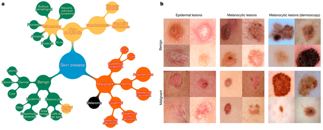
a, A subset of the top of the tree-structured taxonomy of skin disease. The full taxonomy contains 2,032 diseases and is organized based on visual and clinical similarity of diseases. Red indicates malignant, green indicates benign, and orange indicates conditions that can be either. Black indicates melanoma. The first two levels of the taxonomy are used in validation. Testing is restricted to the tasks of b. b, Malignant and benign example images from two disease classes. These test images highlight the difficulty of malignant versus benign discernment for the three medically critical classification tasks we consider: epidermal lesions, melanocytic lesions and melanocytic lesions visualized with a dermoscope. Example images reprinted with permission from the Edinburgh Dermofit Library (https://licensing.eri.ed.ac.uk/i/software/dermofit-image-library.html).

To take advantage of fine-grained information contained within the taxonomy structure, we develop an algorithm (Extended Data Table 1) to partition diseases into fine-grained training classes (for example, amelanotic melanoma and acrolentiginous melanoma). During inference, the CNN outputs a probability distribution over these fine classes. To recover the probabilities for coarser-level classes of interest (for example, melanoma) we sum the probabilities of their descendants (see Methods and Extended Data Fig. 1 for more details).

We validate the effectiveness of the algorithm in two ways, using nine-fold cross-validation. First, we validate the algorithm using a three-class disease partition—the first-level nodes of the taxonomy, which represent benign lesions, malignant lesions and non-neoplastic lesions. In this task, the CNN achieves 72.1 ± 0.9% (mean ± s.d.) overall accuracy (the average of individual inference class accuracies) and two dermatologists attain 65.56% and 66.0% accuracy on a subset of the validation set. Second, we validate the algorithm using a nine-class disease partition—the second-level nodes—so that the diseases of each class have similar medical treatment plans. The CNN achieves 55.4 ± 1.7% overall accuracy whereas the same two dermatologists attain 53.3% and 55.0% accuracy. A CNN trained on a finer disease partition performs better than one trained directly on three or nine classes (see Extended Data Table 2), demonstrating the effectiveness of our partitioning algorithm. Because images of the validation set are labelled by dermatologists, but not necessarily confirmed by biopsy, this metric is inconclusive, and instead shows that the CNN is learning relevant information.

To conclusively validate the algorithm, we tested, using only biopsy-proven images on medically important use cases, whether the algorithm and dermatologists could distinguish malignant versus benign lesions of epidermal (keratinocyte carcinoma compared to benign seborrheic keratosis) or melanocytic (malignant melanoma compared to benign nevus) origin. For melanocytic lesions, we show two trials, one using standard images and the other using dermoscopy images, which reflect the two steps that a dermatologist might carry out to obtain a clinical impression. The same CNN is used for all three tasks. Figure 2b shows a few example images, demonstrating the difficulty in distinguishing between malignant and benign lesions, which share many visual features. Our comparison metrics are sensitivity and specificity:

$$\text{sensitivity}=\frac{\text{true positive}}{\text{positive}}$$

$$\text{specificity}=\frac{\text{true negative}}{\text{negative}}$$

where ‘true positive’ is the number of correctly predicted malignant lesions, ‘positive’ is the number of malignant lesions shown, ‘true negative’ is the number of correctly predicted benign lesions, and ‘negative’ is the number of benign lesions shown. When a test set is fed through the CNN, it outputs a probability, P, of malignancy, per image. We can compute the sensitivity and specificity of these probabilities by choosing a threshold probability t and defining the prediction $\widehat{y}$ for each image as $\widehat{y}=P\ge t$. Varying t in the interval 0–1 generates a curve of sensitivities and specificities that the CNN can achieve.

We compared the direct performance of the CNN and at least 21 board-certified dermatologists on epidermal and melanocytic lesion classification (Fig. 3a). For each image the dermatologists were asked whether to biopsy/treat the lesion or reassure the patient. Each red point on the plots represents the sensitivity and specificity of a single dermatologist. The CNN outperforms any dermatologist whose sensitivity and specificity point falls below the blue curve of the CNN, which most do. The green points represent the average of the dermatologists (average sensitivity and specificity of all red points), with error bars denoting one standard deviation. The area under the curve (AUC) for each case is over 91%. The images for this comparison (135 epidermal, 130 melanocytic and 111 melanocytic dermoscopy images) are sampled from the full test sets. The sensitivity and specificity curves for our entire test set of biopsy-labelled images comprised 707 epidermal, 225 melanocytic and 1,010 melanocytic dermoscopy images (Fig. 3b). We observed negligible changes in AUC (< 0.03) when we compared the sample dataset (Fig. 3a) with the full dataset (Fig. 3b), validating the reliability of our results on a larger dataset. In a separate analysis with similar results (see Methods) dermatologists were asked whether they thought a lesion was malignant or benign.

Figure 3 |. Skin cancer classification performance of the CNN and dermatologists.

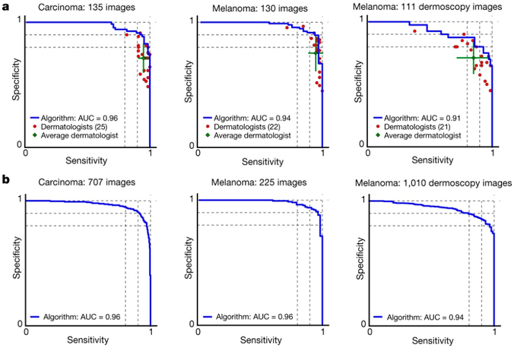
a, The deep learning CNN outperforms the average of the dermatologists at skin cancer classification using photographic and dermoscopic images. Our CNN is tested against at least 21 dermatologists at keratinocyte carcinoma and melanoma recognition. For each test, previously unseen, biopsy-proven images of lesions are displayed, and dermatologists are asked if they would: biopsy/treat the lesion or reassure the patient. Sensitivity, the true positive rate, and specificity, the true negative rate, measure performance. A dermatologist outputs a single prediction per image and is thus represented by a single red point. The green points are the average of the dermatologists for each task, with error bars denoting one standard deviation (calculated from n = 25, 22 and 21 tested dermatologists for keratinocyte carcinoma, melanoma and melanoma under dermoscopy, respectively). The CNN outputs a malignancy probability P per image. We fix a threshold probability t such that the prediction $\widehat{y}$ for any image is $\widehat{y}=P\ge t$, and the blue curve is drawn by sweeping t in the interval 0–1. The AUC is the CNN’s measure of performance, with a maximum value of 1. The CNN achieves superior performance to a dermatologist if the sensitivity–specificity point of the dermatologist lies below the blue curve, which most do. Epidermal test: 65 keratinocyte carcinomas and 70 benign seborrheic keratoses. Melanocytic test: 33 malignant melanomas and 97 benign nevi. A second melanocytic test using dermoscopic images is displayed for comparison: 71 malignant and 40 benign. The slight performance decrease reflects differences in the difficulty of the images tested rather than the diagnostic accuracies of visual versus dermoscopic examination. b, The deep learning CNN exhibits reliable cancer classification when tested on a larger dataset. We tested the CNN on more images to demonstrate robust and reliable cancer classification. The CNN’s curves are smoother owing to the larger test set.

We examined the internal features learned by the CNN using t-SNE (t-distributed Stochastic Neighbour Embedding)²⁹ (Fig. 4). Each point represents a skin lesion image projected from the 2,048-dimensional output of the CNN’s last hidden layer into two dimensions. We see clusters of points of the same clinical classes (Fig. 4, insets show images of different diseases). Basal and squamous cell carcinomas are split across the malignant epidermal point cloud. Melanomas cluster in the centre, in contrast to nevi, which cluster on the right. Similarly, seborrheic keratoses cluster opposite to their malignant counterparts.

Figure 4 |. t-SNE visualization of the last hidden layer representations in the CNN for four disease classes.

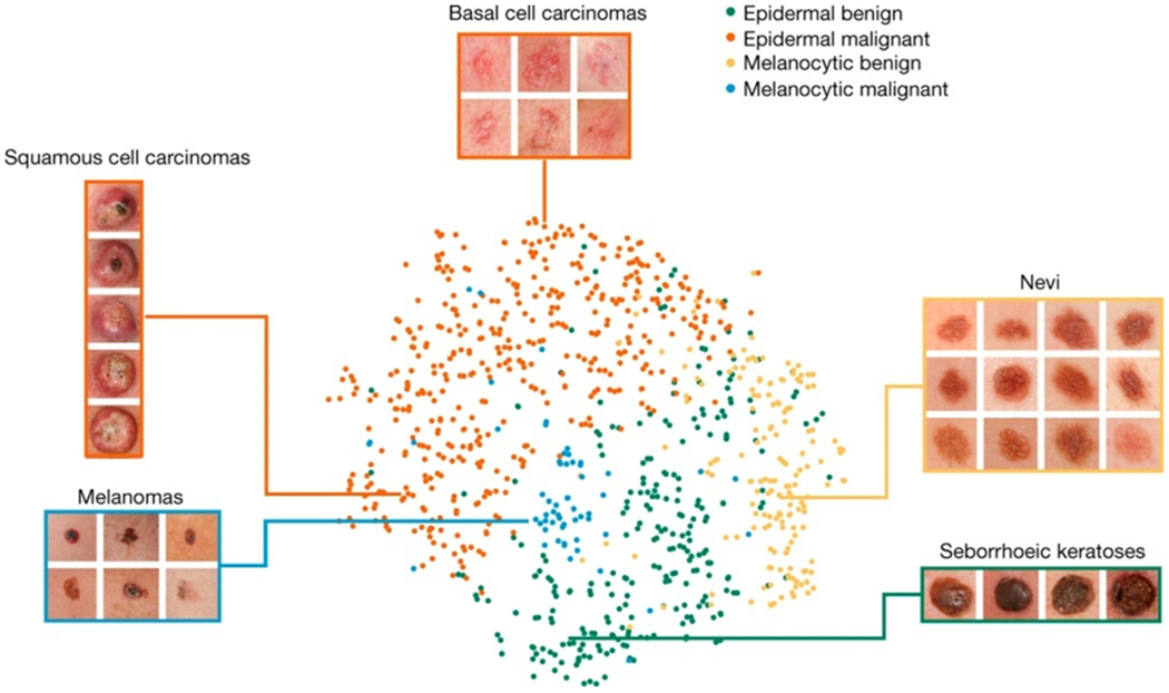
Here we show the CNN’s internal representation of four important disease classes by applying t-SNE, a method for visualizing high-dimensional data, to the last hidden layer representation in the CNN of the biopsy-proven photographic test sets (932 images). Coloured point clouds represent the different disease categories, showing how the algorithm clusters the diseases. Insets show images corresponding to various points. Images reprinted with permission from the Edinburgh Dermofit Library (https://licensing.eri.ed.ac.uk/i/software/dermofit-image-library.html).

Here we demonstrate the effectiveness of deep learning in dermatology, a technique that we apply to both general skin conditions and specific cancers. Using a single convolutional neural network trained on general skin lesion classification, we match the performance of at least 21 dermatologists tested across three critical diagnostic tasks: keratinocyte carcinoma classification, melanoma classification and melanoma classification using dermoscopy. This fast, scalable method is deployable on mobile devices and holds the potential for substantial clinical impact, including broadening the scope of primary care practice and augmenting clinical decision-making for dermatology specialists. Further research is necessary to evaluate performance in a real-world, clinical setting, in order to validate this technique across the full distribution and spectrum of lesions encountered in typical practice. Whilst we acknowledge that a dermatologist’s clinical impression and diagnosis is based on contextual factors beyond visual and dermoscopic inspection of a lesion in isolation, the ability to classify skin lesion images with the accuracy of a board-certified dermatologist has the potential to profoundly expand access to vital medical care. This method is primarily constrained by data and can classify many visual conditions if sufficient training examples exist. Deep learning is agnostic to the type of image data used and could be adapted to other specialties, including ophthalmology, otolaryngology, radiology and pathology.

METHODS

Datasets.

Our dataset comes from a combination of open-access dermatology repositories, the ISIC Dermoscopic Archive, the Edinburgh Dermofit Library²² and data from the Stanford Hospital. The images from the online open-access dermatology repositories are annotated by dermatologists, not necessarily through biopsy. The ISIC Archive data used are composed strictly of melanocytic lesions that are biopsy-proven and annotated as malignant or benign. The Edinburgh Dermofit Library and data from the Stanford Hospital are biopsy-proven and annotated by individual disease names (that is, actinic keratosis). In our test sets, melanocytic lesions include malignant melanomas—the deadliest skin cancer—and benign nevi. Epidermal lesions include malignant basal and squamous cell carcinomas, intraepithelial carcinomas, pre-malignant actinic keratosis and benign seborrheic keratosis.

Taxonomy.

Our taxonomy represents 2,032 individual diseases arranged in a tree structure with three root nodes representing general disease classes: (1) benign lesions, (2) malignant lesions and (3) non-neoplastic lesions (Fig. 2b). It was derived by dermatologists using a bottom-up procedure: individual diseases, initialized as leaf nodes, were merged based on clinical and visual similarity, until the entire structure was connected. This aspect of the taxonomy is useful in generating training classes that are both well-suited for machine learning classifiers and medically relevant. The root nodes are used in the first validation strategy and represent the most general partition. The children of the root nodes (that is, malignant melanocytic lesions) are used in the second validation strategy, and represent disease classes that have similar clinical treatment plans.

Data preparation.

Blurry images and far-away images were removed from the test and validation sets, but were still used in training. Our dataset contains sets of images corresponding to the same lesion but from multiple viewpoints, or multiple images of similar lesions on the same person. While this is useful training data, extensive care was taken to ensure that these sets were not split between the training and validation sets. Using image EXIF metadata, repository specific information and nearest neighbour image retrieval with CNN features, we created an undirected graph connecting any pair of images that were determined to be similar. Connected components of this graph were not allowed to straddle the train/validation split and were randomly assigned to either train or validation. The test sets all came from independent, high-quality repositories of biopsy-proven images—the Stanford Hospital, the University of Edinburgh Dermofit Image Library and the ISIC Dermoscopic Archive. No overlap (that is, same lesion, multiple viewpoints) exists between the test sets and the training/validation data.

Sample selection.

The epidermal, melanocytic and melanocytic-dermoscopic tests of Fig. 3a used 135 (65 malignant, 70 benign), 130 (33 malignant, 97 benign) and 111 (71 malignant, 40 benign) images, respectively. Their counterparts of Fig. 3b used 707 (450 malignant, 257 benign), 225 (58 malignant, 167 benign), and 1,010 (88 malignant, 922 benign) images, respectively. The number of images used for Fig. 3b was based on the availability of biopsy labelled data (that is, malignant melanocytic lesions are exceedingly rare compared to benign melanocytic lesions). These numbers are statistically justified by the standards of the ILSVRC computer vision challenge⁶, which has 50–100 images per class for validation and test sets. For Fig. 3a, 140 images were randomly selected from each set of Fig. 3b, and a non-tested dermatologist (blinded to diagnosis) removed any images of insufficient resolution (although the network accepts image inputs of 299 × 299 pixels, the dermatologists required larger images for clarity).

Disease partitioning algorithm.

The algorithm that partitions the individual diseases into training classes is outlined more extensively in Extended Data Table 1. It is a recursive algorithm, designed to leverage the taxonomy to generate training classes whose individual diseases are clinically and visually similar. The algorithm forces the average generated training class size to be slightly less than its only hyperparameter, maxClassSize. Together these components strike a balance between (1) generating training classes that are overly fine grained and that do not have sufficient data to be learned properly; (2) generating training classes that are too coarse, too data abundant and bias the algorithm towards them. With maxClassSize = 1,000 this algorithm yields a disease partition of 757 classes. All training classes are descendants of inference classes.

Training algorithm.

We use Google’s Inception v3 CNN architecture pretrained to 93.33% top-five accuracy on the 1,000 object classes (1.28 million images) of the 2014 ImageNet Challenge following ref. 9. We then remove the final classification layer from the network and retrain it with our dataset, fine-tuning the parameters across all layers. During training we resize each image to 299 × 299 pixels in order to make it compatible with the original dimensions of the Inception v3 network architecture and leverage the natural-image features learned by the ImageNet pretrained network. This procedure, known as transfer learning, is optimal given the amount of data available.

Our CNN is trained using backpropagation. All layers of the network are fine-tuned using the same global learning rate of 0.001 and a decay factor of 16 every 30 epochs. We use RMSProp with a decay of 0.9, momentum of 0.9 and epsilon of 0.1. We use Google’s TensorFlow³⁰ deep learning framework to train, validate and test our network. During training, images are augmented by a factor of 720. Each image is rotated randomly between 0° and 359°. The largest upright inscribed rectangle is then cropped from the image, and is flipped vertically with a probability of 0.5.

Inference algorithm.

We follow the convention that each node contains its children. Each training class is represented by a node in the taxonomy, and subsequently, all descendants. Each inference class is a node that has as its descendants a particular set of training nodes. An illustrative example is shown in Extended Data Fig. 1, with red nodes as inference classes and green nodes as training classes. Given an input image, the CNN outputs a probability distribution over the training nodes. Probabilities over the taxonomy follow:

$$P\left(u\right)=\sum _{v\in C\left(u\right)}P\left(v\right)$$

where u is any node, P(u) is the probability of u, and C(u) are the child nodes of u. Therefore, to recover the probability of any inference node we simply sum the probabilities of its descendant training nodes. Note that in the validation strategies all training classes are summed into inference classes. However in the binary classification cases, the images in question are known to be either melanocytic or epidermal and so we utilize only the training classes that are descendants of either melanocytic or epidermal classes.

Confusion matrices.

Extended Data Fig. 2 shows the confusion matrix of our method over the nine classes of the second validation strategy (Extended Data Table 2d) in comparison to the two tested dermatologists. This demonstrates the misclassification similarity between the CNN and human experts. Element (i, j) of each confusion matrix represents the empirical probability of predicting class j given that the ground truth was class i. Classes 7 and 8—benign and malignant melanocytic lesions—are often confused with each other. Many images are mistaken as class 6, the inflammatory class, owing to the high variability of diseases in this category. Note how easily malignant dermal tumours are confused for other classes, by both the CNN and dermatologists. These tumours are essentially nodules under the skin that are challenging to visually diagnose.

Saliency maps.

To visualize the pixels that a network is fixating on for its prediction, we generate saliency maps, shown in Extended Data Fig. 3, for example images of the nine classes of Extended Data Table 2d. Backpropagation is an application of the chain rule of calculus to compute loss gradients for all weights in the network. The loss gradient can also be backpropagated to the input data layer. By taking the L1 norm of this input layer loss gradient across the RGB channels, the resulting heat map intuitively represents the importance of each pixel for diagnosis. As can be seen, the network fixates most of its attention on the lesions themselves and ignores background and healthy skin.

Sensitivity–specificity curves with different questions.

In the main text we compare our CNN’s sensitivity and specificity to that of at least 21 dermatologists on the three diagnostic tasks of Fig. 3. For this analysis each dermatologist was asked if they would biopsy/treat the lesion or reassure the patient. This choice of question reflects the actual in-clinic task that dermatologists must perform—deciding whether or not to continue medically analysing a lesion. A similar question to ask a dermatologist, though less clinically relevant, is if they believe a lesion is malignant or benign. The results of this analysis are shown in Extended Data Fig. 4. As in Fig. 3, the CNN is on par with the performance of the dermatologists and outperforms the average. In the epidermal lesions test, the CNN is just above one standard deviation above the average of the dermatologists, and in both melanocytic lesion tests the CNN is just below one standard deviation above the average of the dermatologists.

Use of human subjects.

All human subjects were board-certified dermatologists that took our tests under informed consent. This study was approved by the Stanford Institutional Review Board, under trial registration number 36050.

Data availability statement.

The medical test sets that support the findings of this study are available from the ISIC Archive (https://isic-archive.com/) and the Edinburgh Dermofit Library (https://licensing.eri.ed.ac.uk/i/software/dermofit-image-library.html). Restrictions apply to the availability of the medical training/validation data, which were used with permission for the current study, and so are not publicly available. Some data may be available from the authors upon reasonable request and with permission of the Stanford Hospital.

Extended Data

Extended Data Figure 1 |. Procedure for calculating inference class probabilities from training class probabilities.

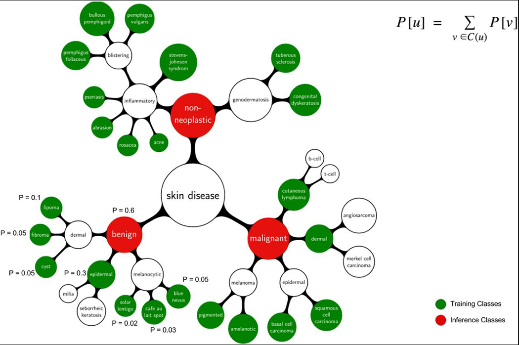
Illustrative example of the inference procedure using a subset of the taxonomy and mock training/inference classes. Inference classes (for example, malignant and benign lesions) correspond to the red nodes in the tree. Training classes (for example, amelanotic melanoma, blue nevus), which were determined using the partitioning algorithm with maxClassSize = 1,000, correspond to the green nodes in the tree. White nodes represent either nodes that are contained in an ancestor node’s training class or nodes that are too large to be individual training classes. The equation represents the relationship between the probability of a parent node, u, and its children, C(u); the sum of the child probabilities equals the probability of the parent. The CNN outputs a distribution over the training nodes. To recover the probability of any inference node it therefore suffices to sum the probabilities of the training nodes that are its descendants. A numerical example is shown for the benign inference class: P_benign = 0.6 = 0.1 + 0.05 + 0.05 + 0.3 + 0.02 + 0.03 + 0.05.

Extended Data Figure 2 |. Confusion matrix comparison between CNN and dermatologists.

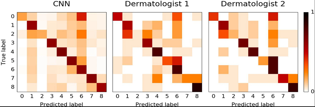
Confusion matrices for the CNN and both dermatologists for the nine-way classification task of the second validation strategy reveal similarities in misclassification between human experts and the CNN. Element (i, j) of each confusion matrix represents the empirical probability of predicting class j given that the ground truth was class i, with i and j referencing classes from Extended Data Table 2d. Note that both the CNN and the dermatologists noticeably confuse benign and malignant melanocytic lesions—classes 7 and 8—with each other, with dermatologists erring on the side of predicting malignant. The distribution across column 6—inflammatory conditions—is pronounced in all three plots, demonstrating that many lesions are easily confused with this class. The distribution across row 2 in all three plots shows the difficulty of classifying malignant dermal tumours, which appear as little more than cutaneous nodules under the skin. The dermatologist matrices are each computed using the 180 images from the nine-way validation set. The CNN matrix is computed using a random sample of 684 images (equally distributed across the nine classes) from the validation set.

Extended Data Figure 3 |. Saliency maps for nine example images from the second validation strategy.

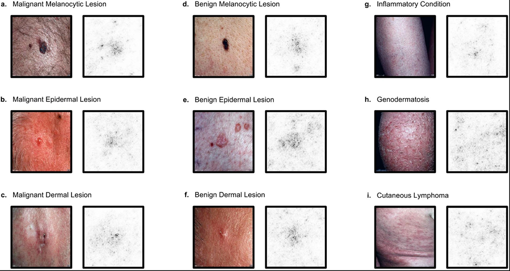
a–i, Saliency maps for example images from each of the nine clinical disease classes of the second validation strategy reveal the pixels that most influence a CNN’s prediction. Saliency maps show the pixel gradients with respect to the CNN’s loss function. Darker pixels represent those with more influence. We see clear correlation between the lesions themselves and the saliency maps. Conditions with a single lesion (a–f) tend to exhibit tight saliency maps centred around the lesion. Conditions with spreading lesions (g–i) exhibit saliency maps that similarly occupy multiple points of interest in the images. a, Malignant melanocytic lesion (source image: https://www.dermquest.com./imagelibrary/large/020114HB.JPG). b, Malignant epidermal lesion (source image: https://www.dermquest.com/imagelibrary/large/001883HB.JPG). c, Malignant dermal lesion (source image: https://www.dermquest.com/imagelibrary/large/019328HB.JPG). d, Benign melanocytic lesion (source image: https://www.dermquest.com/imagelibrary/large/010137HB.JPG). e, Benign epidermal lesion (source image: https://www.dermquest.com/imagelibrary/large/046347HB.JPG). f, Benign dermal lesion (source image: https://www.dermquest.com/imagelibrary/large/021553HB.JPG). g, Inflammatory condition (source image: https://www.dermquest.com/imagelibrary/large/030028HB.JPG). h, Genodermatosis (source image: https://www.dermquest.com/imagelibrary/large/030705VB.JPG). i, Cutaneous lymphoma (source image: https://www.dermquest.com/imagelibrary/large/030540VB.JPG).

Extended Data Figure 4 |. Extension of Figure 3 with a different dermatological question.

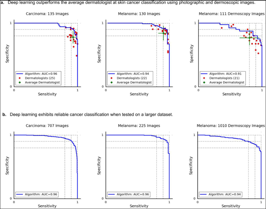
a, Identical plots and results as shown in Fig. 3a, except that dermatologists were asked if a lesion appeared to be malignant or benign. This is a somewhat unnatural question to ask, in the clinic, the only actionable decision is whether or not to biopsy or treat a lesion. The blue curves for the CNN are identical to Fig. 3. b, Figure 3b reprinted for visual comparison to a.

Extended Data Table 1 |.

Disease-Partitioning Algorithm

Algorithm 1 Disease Partitioning Algorithm
1:	Inputs
2:	taxonomy (tree): the disease taxonomy
3:	maxClassSize (int): maximum data points in a class
4:	Output
5:	partition (list of sets): partition of the diseases into classes
6:
7:	procedure Descendants(node)
8:	return {node} ∪ {Descendants(child) for child in node.children}
9:
10:	procedure NumImages(nodes)
11:	return sum(length(node.images) for node in nodes)
12:
13:	procedure PartitionDiseases(node)
14:	class ← Descendants (node)
15:	if NumImages(class) < maxClassSize then
16:	append class to partition
17:	else
18:	for child in node.children do
19	PartitionDiseases(child)
20:
21:	partition ← [ ]
22:	PartitionDiseases (taxonomy.root)
23:	return partition

This algorithm uses the taxonomy to partition the diseases into fine-grained training classes. We find that training on these finer classes improves the classification accuracy of coarser inference classes. The algorithm begins with the top node and recursively descends the taxonomy (line 19), turning nodes into training classes if the amount of data contained in them (with the convention that nodes contain their children) does not exceed a specified threshold (line 15). During partitioning, the recursive property maintains the taxonomy structure, and consequently, the clinical similarity between different diseases grouped into the same training class. The data restriction (and the fact that training data are fairly evenly distributed amongst the leaf nodes) forces the average class size to be slightly less than maxClassSize. Together these components generate training classes that leverage the fine-grained information contained in the taxonomy structure while striking a balance between generating classes that are overly fine-grained and do not have sufficient data to be learned properly, and classes that are too coarse, too data abundant and that prevent the algorithm from properly learning less data-abundant classes. With maxClassSize = 1,000 this algorithm yields 757 training classes.

Extended Data Table 2 |.

General validation results

a.	Classifier	Three-way accuracy	b.	Classifier	Nine-way accuracy
	Dermatologist 1	65.6%		Dermatologist 1	53.3%
	Dermatologist 2	66.0%		Dermatologist 2	55.0%
	CNN	69.4 ± 0.8%		CNN	48.9 ± 1.9%
	CNN - PA	72.1 ± 0.9%		CNN-PA	55.4 ± 1.7%
c.	Disease classes: three-way classification		d.	Disease classes: nine-way classification
	0. Benign single lesions			0. Cutaneous lymphoma and lymphoid infiltrates
	1. Malignant single lesions			1. Benign dermal tumors, cysts, sinuses
	2. Non-neoplastic lesions			2. Malignant dermal tumor
				3. Benign epidermal tumors, hamartomas, milia, and growths
				4. Malignant and premalignant epidermal tumors
				5. Genodermatoses and supernumerary growths
				6. Inflammatory conditions
				7. Benign melanocytic lesions
				8. Malignant Melanoma

Here we show ninefold cross-validation classification accuracy with 127,463 images organized in two different strategies. In each fold, a different ninth of the dataset is used for validation, and the rest is used for training. Reported values are the mean and standard deviation of the validation accuracy across all n = 9 folds. These images are labelled by dermatologists, not necessarily through biopsy; meaning that this metric is not as rigorous as one with biopsy-proven images. Thus we only compare to two dermatologists as a means to validate that the algorithm is learning relevant information. a, Three-way classification accuracy comparison between algorithms and dermatologists. The dermatologists are tested on 180 random images from the validation set—60 per class. The three classes used are first-level nodes of our taxonomy. A CNN trained directly on these three classes also achieves inferior performance to one trained with our partitioning algorithm (PA). b, Nine-way classification accuracy comparison between algorithms and dermatologists. The dermatologists are tested on 180 random images from the validation set—20 per class. The nine classes used are the second-level nodes of our taxonomy. A CNN trained directly on these nine classes achieves inferior performance to one trained with our partitioning algorithm. c, Disease classes used for the three-way classification represent highly general disease classes. d, Disease classes used for nine-way classification represent groups of diseases that have similar aetiologies.

References

- 1.American Cancer Society. Cancer facts & figures 2016. Atlanta, American Cancer Society; 2016. http://www.cancer.org/acs/groups/content/@research/documents/document/acspc-047079.pdf. [Google Scholar]
- 2.Rogers HW et al. Incidence estimate of nonmelanoma skin cancer (keratinocyte carcinomas) in the US population, 2012. JAMA Dermatology 151.10, 1081–1086 (2015). [DOI] [PubMed] [Google Scholar]
- 3.Stern RS Prevalence of a history of skin cancer in 2007: results of an incidence-based model. Arch. Dermatol 146, 279–282 (2010). [DOI] [PubMed] [Google Scholar]
- 4.LeCun Y, Bengio Y & Hinton G Deep learning. Nature 521, 436–444 (2015). [DOI] [PubMed] [Google Scholar]
- 5.LeCun Y & Bengio Y In The Handbook of Brain Theory and Neural Networks (ed. Arbib MA) 3361.10 (MIT Press, 1995). [Google Scholar]
- 6.Russakovsky O et al. Imagenet large scale visual recognition challenge. Int. J. Comput. Vis 115, 211–252 (2015). [Google Scholar]
- 7.Krizhevsky A, Sutskever I & Hinton GE Imagenet classification with deep convolutional neural networks. Adv. Neural Inf. Process. Syst 25, 1097–1105 (2012). [Google Scholar]
- 8.Ioffe S & Szegedy C Batch normalization: accelerating deep network training by reducing internal covariate shift. Proc. 32nd Int. Conference on Machine Learning 448–456 (2015). [Google Scholar]
- 9.Szegedy C, Vanhoucke V, Ioffe S, Shlens J & Wojna Z Rethinking the inception architecture for computer vision. Preprint at https://arxiv.org/abs/1512.00567 (2015). [Google Scholar]
- 10.Szegedy C et al. Going deeper with convolutions. Proc. IEEE Conference on Computer Vision and Pattern Recognition1–9 (2015). [Google Scholar]
- 11.He K, Zhang X, Ren S & Sun J Deep residual learning for image recognition. Preprint at https://arxiv.org/abs/1512.03385 (2015). [Google Scholar]
- 12.Masood A & Al-Jumaily AA Computer aided diagnostic support system for skin cancer: a review of techniques and algorithms. Int. J. Biomed. Imaging 2013, 323268 (2013). [DOI] [PMC free article] [PubMed] [Google Scholar]
- 13.Cerwall P & Report EM Ericssons mobility report https://www.ericsson.com/res/docs/2016/ericsson-mobility-report-2016.pdf (2016). [Google Scholar]
- 14.Rosado B et al. Accuracy of computer diagnosis of melanoma: a quantitative meta-analysis. Arch. Dermatol 139, 361–367, discussion 366 (2003). [DOI] [PubMed] [Google Scholar]
- 15.Burroni M et al. Melanoma computer-aided diagnosis: reliability and feasibility study. Clin. Cancer Res 10, 1881–1886 (2004). [DOI] [PubMed] [Google Scholar]
- 16.Kittler H, Pehamberger H, Wolff K & Binder M Diagnostic accuracy of dermoscopy. Lancet Oncol. 3, 159–165 (2002). [DOI] [PubMed] [Google Scholar]
- 17.Codella N et al. In Machine Learning in Medical Imaging (eds Zhou L, Wang L, Wang Q & Shi Y) 118–126 (Springer, 2015). [Google Scholar]
- 18.Gutman D et al. Skin lesion analysis toward melanoma detection. International Symposium on Biomedical Imaging (ISBI), (International Skin Imaging Collaboration (ISIC), 2016). [Google Scholar]
- 19.Binder M et al. Epiluminescence microscopy-based classification of pigmented skin lesions using computerized image analysis and an artificial neural network. Melanoma Res. 8, 261–266 (1998). [DOI] [PubMed] [Google Scholar]
- 20.Menzies SW et al. In Skin Cancer and UV Radiation (eds Altmeyer P, Hoffmann K & Stücker M) 1064–1070 (Springer, 1997). [Google Scholar]
- 21.Clark WH, et al. Model predicting survival in stage I melanoma based on tumor progression. J. Natl Cancer Inst 81, 1893–1904 (1989). [DOI] [PubMed] [Google Scholar]
- 22.Schindewolf T et al. Classification of melanocytic lesions with color and texture analysis using digital image processing. Anal. Quant. Cytol. Histol 15, 1–11 (1993). [PubMed] [Google Scholar]
- 23.Ramlakhan K & Shang Y A mobile automated skin lesion classification system. 23rd IEEE International Conference on Tools with Artificial Intelligence (ICTAI) 138–141 (2011). [Google Scholar]
- 24.Ballerini L et al. In Color Medical Image Analysis. (eds, Celebi ME & Schaefer G) 63–86 (Springer, 2013). [Google Scholar]
- 25.Deng J et al. Imagenet: A large-scale hierarchical image database. EEE Conference on Computer Vision and Pattern Recognition248–255 (CVPR, 2009). [Google Scholar]
- 26.Mnih V et al. Human-level control through deep reinforcement learning. Nature 518, 529–533 (2015). [DOI] [PubMed] [Google Scholar]
- 27.Silver D et al. Mastering the game of Go with deep neural networks and tree search. Nature 529, 484–489 (2016). [DOI] [PubMed] [Google Scholar]
- 28.Pan SJ & Yang Q A survey on transfer learning. IEEE Trans. Knowl. Data Eng 22, 1345–1359 (2010). [Google Scholar]
- 29.Van der Maaten L, & Hinton G Visualizing data using t-SNE. J. Mach. Learn. Res 9, 2579–2605 (2008). [Google Scholar]
- 30.Abadi M et al. Tensorflow: large-scale machine learning on heterogeneous distributed systems. Preprint at https://arxiv.org/abs/1603.04467 (2016). [Google Scholar]
Associated Data
This section collects any data citations, data availability statements, or supplementary materials included in this article.