

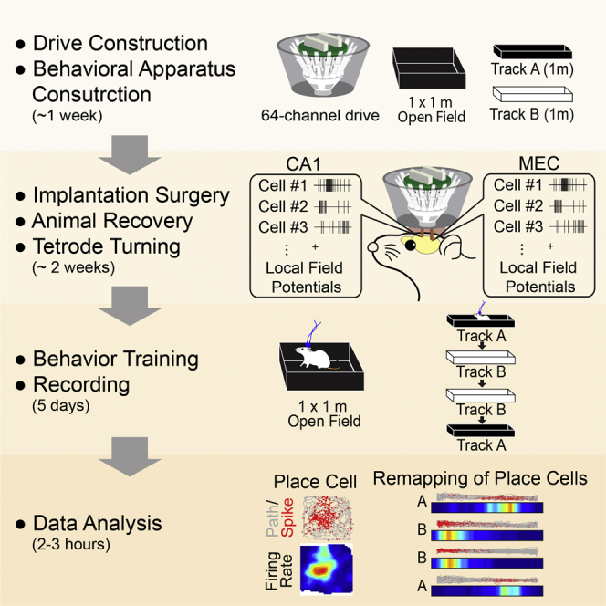
Summary
Hippocampal place cells and entorhinal grid cells exhibit distinct spike patterns in different environments called “remapping,” and we have recently shown that remapping of place cells becomes disrupted in a mouse model of Alzheimer's disease. Here, we describe our protocol for investigating remapping of place cells and grid cells using a custom-made electrophysiology device, with detailed descriptions and problem-solving tips for the construction and implantation of the recording device. We also provide steps for behavioral training, recording, and data analysis.
For complete details on the use and execution of this protocol, please refer to Jun et al. (2020).
Subject areas: Model Organisms, Neuroscience, Behavior
Graphical abstract
Highlights
-
•
Build behavior apparatuses for remapping experiment and construct microdrives
-
•
Implant drives, monitor animal recovery, and perform tetrode turning
-
•
Perform behavior training followed by recording on fifth day
-
•
Analyze data to identify place cells and evaluate degree of remapping
Hippocampal place cells and entorhinal grid cells exhibit distinct spike patterns in different environments called “remapping,” and we have recently shown that remapping of place cells becomes disrupted in a mouse model of Alzheimer's disease. Here, we describe our protocol for investigating remapping of place cells and grid cells using a custom-made electrophysiology device, with detailed descriptions and problem-solving tips for the construction and implantation of the recording device. We also provide steps for behavioral training, recording, and data analysis.
Before you begin
In this protocol, we describe a method for investigating remapping using a knock-in mouse model for Alzheimer’s disease (APPNL-G-F model, (Saito et al., 2014)). Our method can be applied to any mouse models for testing remapping of place cells. All procedures were conducted in accordance with the guidelines of the National Institutes of Health and approved by the Institutional Animal Care and Use Committee at the University of California, Irvine. Mice aged between 3- to 12-month-old were used for our experiments, and similar number of female and male mice was used.
Key resources table
a Open Field Box and Linear Tracks
b Animal surgery + implantation (Geiger et al., 2008)
c Microdrive materials
Step-by-step method details
Construction of behavioral testing enclosures
Timing: 2–4 days
-
1.Prepare following apparatuses (Figure 1):
-
a.1 m2 box (or 80 cm2 box) made of black acryl and a polarizing white cue card (216 mm × 280 mm)
-
i.Acquire following materials for the construction (See key resources table for details): acryl sheet plexiglass plastic with non-glare surface on one side, bolt-together framing, and screws + nuts.
-
ii.Cut the acryl plexiglass into four 30 cm × 80 cm sheets
-
iii.Align the sheets perpendicularly (non-glare surface inside) with bolt-together frames and drill two holes (3/8” diameter) on the corners of each sheet.
-
iv.Form open field box and secure corners by fastening the screw and nuts on bolt-together frame.
-
v.Attach white paper (letter size) on one of the walls as a visual cue.
-
vi.A rubber mat (used in upside-down) is used for a bottom of the open field.Note: Make sure to have the non-glare surface facing inside the box so that there is no reflection during training/recording session.
-
i.
-
b.Two 1-m long linear tracks:
-
i.Acquire following materials for the construction (See key resources table for details): acryl sheet plexiglass plastic with non-glare surface and aluminum 90° frame.
-
ii.For linear track A, cut the acryl plexiglass into three 10 cm × 100 cm sheets and two 10 cm × 10 cm sheets. Form linear track by securing the corners between the sheets using the 90° aluminum frames and attaching through epoxy. Attach white visual cues on the inner walls of black linear track. Cut the rubber mat and put it as flooring for unique tactile cue.
-
iii.For linear track B, repeat as above. However, cover the entire inner walls with non-reflective white sheets (See key resources table) and use black marker to draw unique pattern of visual cues. Lastly, cover the floor with white sandpaper for unique tactile cue.
-
i.
-
a.
Figure 1.

Preparation for open field box and linear tracks
(A and B) (A) Construct open field box (1 m × 1 m or 80 cm × 80 cm) and (B) linear tracks (1 m) from black acryl board. Make sure that one of the surfaces has a matte finish to reduce reflected light. Use appropriate bolt together frames from McMaster-Carr to build stable and secure box and tracks.
Electrode and surgery preparation
Construct and surgically implant a multielectrode drive for electrophysiological recordings.
-
2.Construct a custom-built 64-channel drive as described previously (Brunetti et al., 2014, Liang et al., 2017) to target the CA1 of the hippocampus and superficial layer of the medial entorhinal cortex (MEC) (Figure 2)
-
a.Form 6 cm 2 × 2 bundle with outer polymide (30G) tubing.Note: Try to minimize the gap between each polymide tubing to minimize the size of the bundle.
-
b.Cut this bundle at the middle to create two 3 cm 2 × 2 bundles. (One will be used for CA1 of the hippocampus and another will be used for MEC)
-
c.Two separate bundles, with one targeting CA1 of the hippocampus and another targeting the medial entorhinal cortex, are separated by a distance of 2.5–2.7 mm with height difference 0.8–1.2 mm.Note: Attach these bundles to the core using the sticky rubber and little by little modify their positions manually until desired positions are achieved.
-
d.Affix the bundles with position mentioned above to the drive core using epoxy and cure overnight to ensure epoxy is completely fixed.
-
e.Place the spring and shuttle through shaft of microscrew and screw it down to four holes on each side. Have each microscrew placed apart by at least one hole so that they are evenly spread out.Note: There are eight holes on each side, but only four holes will be used, because there will be eight tetrodes inserted (double packing) into four cannulas. In contrast to previous work (Liang et al., 2017) where 34G was used to create the bundle, we use 30G as this is the smallest and durable tubing that we can get it to work without getting it bent during turning.
-
f.Prepare at least eight 0.5 cm anchor polymide (20G) tubing and thread this through each outer tubing (34G). Bring the anchor tubing (20G) and place it inside the guide hole located front of each screw to align outer tubing (30G) to each shuttle. Affix the position of anchoring tube with epoxy.
-
g.Prepare at least eight 3 cm inner polymide (34G) tubing and thread them through outer tubing (30G) and have the 34G tubing affixed to the shuttle using epoxy (Figure 2C).Note: Pay close attention to determine whether inner tubing (34G) can smoothly thread through the outer tubing (30G). There should be no bending nor extra force needed to push inner tubing (34G) through the outer tubing (30G). If any bending is noticed, repeat step e-g at unused adjacent holes for replacement.
-
h.Attach the 64-channel EIB board on top of the drive core.
-
i.Thread tetrodes through inner tubing and connect to the EIB board using gold pins. Place two tetrodes per tubing.
-
j.Watch the protocol video for more details (Brunetti et al., 2014):
-
a.
Figure 2.

Microdrive construction
(A) Assemble custom-built 64-channel Microdrive (Liang et al., 2017). Bases and shuttles are custom 3D printed. Shielding cones are built using transparency sheet epoxied to aluminum foil.
(B) Surgical scheme illustrating the location of tetrodes to be implanted in CA1 of hippocampus and layer II/III of medial entorhinal cortex.
(C) Scheme of outer (34G), inner (30G), and guide (20G) polyamide tubing during drive assembly.
Implantation surgery
The description below is a method specific to drive implantation in mice. For those who are not familiar to general survival surgery in rodents, watch a video in Geiger et al. (Geiger et al., 2008).
-
3.Implantation Surgery
-
a.Begin anesthetizing animals by placing them inside an induction chamber with 2%–3% isoflurane mixed with oxygen flow 0.8–1.0 L/min.
-
b.Administer subcutaneous injections of buprenorphine (working solution 0.015 mg/mL; dose 0.2 mL/20 g) at the start of surgery.
-
c.Place animals on stereotaxic stage with correct ear bar placement for head fixation.
-
d.Continue anesthetizing mice with reduced isoflurane content (oxygen flow: 0.8–1.0 L/min, 1%–1.5% isoflurane)
-
e.Animal’s temperature is closely monitored and regulated at 37.0°C throughout the surgery using the thermoregulator system.
-
f.Perform a craniotomy that is sufficiently large for electrode implantation (1.5 mm × 1.5 mm) (Figures 3 and 4)
-
i.Fix the head of the mouse in a stereotaxic frame.
-
ii.Shave hair on the surgical site using hair clipper, followed by disinfection.
-
iii.Make a small incision along the sagittal line of the skull.
-
iv.Locate and record Bregma and Lambda coordinates. Make sure the height difference between these two sites is less than 100 μm by adjusting head position.
-
v.Mark the desired stereotaxic coordinate for electrode implantation.Note: Craniotomy is centered at AP 2.5 mm ML 2.5 mm from Bregma for the hippocampus (approximately 1.5 × 1.5 mm) and 0.3–0.5 mm anterior to transverse sinus and ML 3.5 mm from midline for medial entorhinal cortex (approximately 1.5 × 1.5 mm).Note: The Transverse Sinus is a landmark that can be used to estimate the position of MEC. It can only be identified by thinning the skull near the lambdoid suture. Once the skull is thinned enough to be transparent, rinsing with saline should be able to help with locating and visualizing the Transverse Sinus. Since this vessel is prone to rupture and can cause a lot of bleeding, take extra precaution when removing the dura on top of this vessel. Do not pierce the transverse sinus as it is a landmark. Be prepared to stop bleeding using Surgifoam, bone wax or warm saline.
-
i.
-
g.Make a Burr hole (0.5 mm diameter) for T1 ground screw using a small (0.5 mm tip) drill (above left cerebellum)
-
h.Temporarily protect the three holes by applying Kwik-Sil.
-
i.Use the Metabond kit for securing the custom-built titanium headplate on (Oval shaped ring with inner diameter 9 mm × 10.169 mm with bottom ring width 1 mm and top ring width 1.412 mm ; ring thickness of 0.794 mm) top of skull.Note: We use the headplate for stably anchoring the drive to mouse skull for chronic in vivo recording. In addition, this can act as a platform in which dental cement can be applied around to anchor the drive to the skull without having it flowing out to unwanted skin areas. Metabond cement is quickly cured and is ideal for fixing headplate to the skull. (Design sheet available: http://www.igarashilab.org/resource)
-
j.Apply enamel etchant (red) for 30–60 s, then wipe it with q-tips and wash with saline. Create a rough surface by scoring with tip of forceps.
-
k.Completely wipe the surface of the skull and make sure it is dry before placing the headplate.
-
l.Mix the quick base, catalyst and cement powder in the tray and apply this mixture between the skull and headplate.
-
m.Seal the gap between the headplate and the skull by applying at the edges of inner ring of headplate.
-
n.Slowly apply more mixture to completely cover the skull and headplate. Make sure to avoid putting any mixture on top of holes covered with Kwik-Sil (if this occurs, gently scrape away the mixture to uncover holes before solidifying)
-
o.(Wait for ∼5 min to completely fix)Note: During steps i through n, make sure that Kwik-Sil protecting the holes remains secure and intact.
-
p.Remove the Kwik-Sil to expose the holes for implantation.
-
q.Remove the dura for all three holes using fine forceps. Prepare to stop bleeding using bone wax, Surgifoam or warm saline.
-
r.Insert T1 screw into the cerebellum. Hook up a looped, exposed side of ground wire on the screw. Apply a silver paint and wait until it gets dried. Cover and secure the screw by applying Coldpac dental cement. (Wait for ∼10 min to completely fix)
-
s.Bring down the drive and make sure the bundles align and fit to the two holes (one for CA1 and another for MEC). Record the height at which the bundles are contacting the surface of brain and retract vertically ∼3 mm.
-
t.Apply Surgilube around the bundles, which will protect tetrodes from contacting the dental cement in subsequent steps.
-
u.Bring down the drive back to the recorded height at which bundles contact the surface of brain and apply Coldpac dental cement to secure the drive to the headplate and the skull.
-
v.Disinfect the exposed area between dental cement and edge of the skin with iodine before closing the wound. Then apply 70% ethanol outside of surgical sites around the skin for disinfection.
-
w.Close the wound by attaching the skin to headplate using Vetbond. (Figure 5)Note: During any dental cement placement, make sure to avoid any protrusion from the headplate. This will significantly affect animal’s recovery.
-
a.
Figure 3.

Craniotomy at the CA1 and MEC for electrode implantation
(A) Craniotomy performed at the CA1 of the hippocamprus and MEC. CA1 hole was drilled at AP 2.5 mm and ML 2.5 mm from Bregma, and MEC hole was drilled 0.3–0.5 mm anterior to Transverse Sinus and ML 3.5 mm from midline.
(B) Magnified view of exposed surface of holes drilled for CA1 and MEC. Dotted line indicates boundary of transverse sinus. A hole for the ground screw is also drilled above the left cerebellum (not shown).
Figure 4.

Insertion of the multi-electrode drive at the CA1 of the hippocampus and MEC and dental cement application
Holes are protected with Kwik-Sil before applying the dental cement. (Top, second left) Mouse skull with headplate placement (Top second right) followed by smooth layering of dental cement around the CA1, MEC, and ground screw (Top right) before drive implantation. Ground screw is placed in the cerebellum followed by hooking with ground wire (Middle, from left to right) (Bottom, from left to right) Lowering of the tetrodes onto the surface of the CA1 and MEC. Placement of surgical lube around tetrodes to prevent exposure to dental cement. Sufficient layering of dental cement around the headplate and tetrodes. Final application of dental cement to completely cover and fix the skull to the drive.
Figure 5.

Completed multi-electrode drive implantation
Finish implantation with a coat of iodine around the surgery site and Vetbond tissue adhesive surrounding the headplate. Make sure to avoid any caudally protruding dental cement.
Postoperative recovery
Allow operated mice to rest for at least 5 days before experimentation.
Note: Monitor animals’ weight and body condition score (BCS) every day after the surgery. Animals should fully recover before beginning the training. Animals’ body weight should return to their original plus drive weight and their BCS should be three.
CRITICAL: If the animals take longer than 10 days to recover, there are potential health issues that need to be closely addressed. The two most frequently occurring issues are chronic infection and excess dental cement protruding caudally from the headplate. Excess dental cement will cause pain when the animal is trying to extend their neck backwards, resulting in limited movement and delayed recovery. (See problem 1)
-
4.
Tetrodes need to be turned daily (more than 40 μm) to ensure that they do not get stuck in the position before reaching the target of interest. Make sure to keep track of the distance that tetrodes traveled in a separate log sheet. Maintaining a good record of tetrode position (depth), as well as the number of units obtained from each tetrode is critical for estimating the position of tetrodes in the brain.
-
5.
Connect tetrodes to a multichannel, impedance matching, unity gain headage (Neuralynx) daily to check for cluster units.
Note: The output of the headstage was connected to a data acquisition system (Neuralynx).
-
6.Advance the tetrodes daily until they reach 1200–1600 μm for CA1 pyramidal cells and 1200–1800 μm for MEC grid cells. Record from neurons detected by tetrodes in open field session at least once a day. Run firing field analysis (see details in ‘data collection and analysis’ section). This will assist with identifying place cells and grid cells. (See Figure 6 for representative clusters)
-
a.Place cells should have a clear firing field in a defined area.
-
b.Grid cells should have clear hexagonal pattern of firing fields.
-
a.
-
7.CA1 pyramidal cell layer can be identified based on their unique physiological properties, particularly their autocorrelation.
-
a.There are prominent autocorrelation peaks within 10 milliseconds from the time zero of the autocorrelogram. This is known as complex-spike firing pattern. (Csicsvari et al., 1999, Ranck, 1973, Renshaw et al., 1940)
-
b.Some neurons in CA1 are modulated by theta oscillation, observed as repetitive peaks in every ∼110 ms in the autocorrelogram.
-
a.
-
8.
Superficial neurons in the MEC are also strongly modulated by theta and this can be identified in the spike autocorrelation. (Fyhn et al., 2004) In addition, stronger theta power will be detected in the local field potentials as the tetrode traverses the border from postrhinal cortex to the MEC.
-
9.
Stop turning when place cells or grid cells are detected from the tetrodes.
Figure 6.

Example clusters during recording session
(A) Example of spike sorting in energy space to identify single units across sessions, demonstrating stable chronic recording across sessions.
(B) Autocorrelogram of cell 1. Note the theta-phase tuned peaks.
(C) Close-up autocorrelogram of cell 1. Note sharp peaks between 0 to ± 10 ms indicating bursts.
Behavioral testing and recording
Once the animals fully recover, they will be food restricted until their body weight is reduced to 85% of their original weight. This is done to motivate the animals to explore toward cookie crumbs during the training/recording session.
-
10.Training (Figure 7)
-
a.In the open field task, motivate exploration by throwing cookie crumbs randomly throughout the enclosure. Each session should last between 15 – 20 min.
-
b.Upon finishing the open field task, rest animals for 5 min in the home cage.
-
c.Next, train animals in the remapping task by having them run in 1-m long linear tracks. During this task, animals are required to run in successive series of Track A → Track B → Track B → Track A. Two tracks need to be placed in the same room. Between the sessions, give animals 5 min rest in a home cage. Motivate running by placing cookie crumbs on the end positions of the linear tracks. Each session should last between 5 to 10 min. On the linear tracks, the mice need to run at least 10 full laps (back and forth).
-
a.
-
11.Recording
-
a.On the fifth day of training, record units throughout the experiment.
-
b.Make sure to input timestamps into the recording system between the sessions. i.e.,) ‘Openfield begins’, ‘Openfield ends,’ ‘Track A – first begins’, ‘Track A – first ends’, and so on…
-
c.For spike data collection, amplify unit activity by a factor of 3000–5000 and band-pass filter from 600 Hz to 6000 Hz. Set the threshold for spike waveforms around 25–55 μV. In our case using Neuralynx, the units are time-stamped and digitized at 32 kHz for 1 ms.
-
d.Track the position of animal using two light-emitting diodes (LEDs), one large and one small, on the head stage (sampling rate 50 Hz) by means of an overhead video camera.
-
a.
Figure 7.

Linear track training
Animals are trained to run back and forth in the linear tracks at least 10 laps per session. (Left) All training is performed under dim light. (Right) Representative training session in linear track A is shown with illumination for visualization.
Data analysis
-
12.Perform spike sorting offline using graphical cluster-cutting softwares. We use a traditional cluster cutting software MClust by Dr. David Redish (https://redishlab.umn.edu/mclust) (Redish, 2020). Several automatic clustering softwares are currently available such as KlustaKwik or Kilosort (Chung et al., 2017, Kadir et al., 2014, Pachitariu et al., 2016, Rossant et al., 2016).
-
a.In MClust, manually identify the clusters from two-dimensional projections with parameter space representing waveform amplitude, energy, and peak to valley difference. Track same cluster across all sessions within a day by calculating the L-ratio and isolation distance. (Schmitzer-Torbert et al., 2005)
-
a.
-
13.Distinguish putative excitatory cells from putative interneurons by spike peak-to-valley width and average rate. (Bartho et al., 2004). (Figure 8)
-
a.Choose a channel that has the largest peak-to-valley amplitude from four channels of each tetrode. Using this channel, calculate the peak-to-valley duration of the spike (peak-to-valley width). Plot the distribution of peak-to-valley width for all recorded neurons (Figure 8). There will be a bimodal distribution of the width, and the threshold for defining putative excitatory cells can be set at the boundary of the two peaks. In our case, the threshold was at 230 μs. We also used the threshold of mean firing rates of more than 0.1 Hz to remove cells with very few spikes.
-
b.Define putative interneurons with spike-peak-valley width of less than 230 μs.For a practical example of the data analysis, we share spike files and MATLAB codes used in our previous report (Jun et al., 2020). Visit http://www.igarashilab.org/resource (Igarashi, 2021) and download the following files in your desired folder:
-
i.One hundred and ten spike files (in “spikeFiles∗.mat” format. This data set contains 62 CA1 neurons from WT mice and 48 CA1 neurons in APP-KI mice).Data structure of spikeFiles:
Structure name: Description: DataS01 Data from the 1 m open field box DataS02 Data from Track A (first session in Track A) DataS03 Data from Track B (first session in Track B) DataS04 Data from Track B (second session in Track B) DataS05 Data from Track A (second session in Track A) Each data structure contains following structure fields:Structure name: Description: spikeTimeStamp time stamp of spikes (in second) PositionTS time stamp of animal position data (in second) PositionX animal position in X-axis PositionY animal position in Y-axis -
ii.Three MATLAB codes
Code name: Description: boxSpikeInfo3.m This code analyzes spikes in the open field analyze4LinearTracks.m This code analyzes spikes in the linear track analyzePopulationVector.m This code calculates population vector correlation
-
i.
-
a.
Figure 8.

Distribution of principal neurons
Electrophysiological features for classifying putative principal neurons. Peak to valley time of spike waveform was used to distinguish putative interneurons from principal neurons. Peak to valley time of spike waveform was used to distinguish putative interneurons from principal neurons in CA1 (A, top) and MEC (B, top). Dashed line (230 μs) represents cut off for interneuron to principal neuron classification (Bartho et al., 2004). No difference was observed for the distribution of peak to valley time between WT and APP-KI mice for both CA1 neurons and MEC neurons (KS test, p >0.05). (A, bottom- B, bottom) Same data, but were plotted for average firing rate in y-axis. Individual neurons were plotted as triangle (WT) or circle (APP-KI). The plot shows high firing rate for putative interneurons below the 230 μs cut line. (C) Left: Spike wave form representing principal neuron. Right: Spike wave form representing interneuron.
-
14.
Analysis of spikes in the open field box (Figure 9)
Run boxSpikeInfo3.m in MATLAB-
a.This code collects spike data from an individual cell that is aligned to animal’s position during the open field box recording session.
-
b.Position data is sorted into 2.5 cm × 2.5 cm bins.
-
c.For smoothing the path, 21-sample boxcar window filter is applied.
-
d.Firing rate distribution is determined by counting the number of spikes in each bin as well as the time spent per bin.
-
e.For smoothing the firing map, boxcar average over the surrounding 5 × 5 bins is applied.
-
f.For each cell, the following data are extracted:
-
i.Plot showing animal’s path and spikes
-
ii.Two-dimensional firing rate map
-
iii.Adapted firing rate map
-
iv.Shannon’s Spatial Information Score (bits/spike)
-
v.Mean Firing Rate
-
vi.Peak Firing Rate (highest firing rate observed in any bin from smoothed map)Note: Spatial Information Score is a metric for assessing the degree of spatial representation of individual neurons (Skaggs et al., 1992). We used Spatial Information Score for defining place cells, by calculating the distribution of Spatial Information Score in the randomly shuffled data (see Figure 1K, (Jun et al., 2020)). Mean firing rate and peak firing rate are also important metrics to judge if spiking activity is impaired or not in your animal models.
-
i.
-
a.
Figure 9.

Example place cell from WT and CA1 neuron from APP-KI from 1×1 m open field
Top: Red dots and gray lines denote spike position and animal trace in the 1×1 m open field, respectively. Bottom: Firing rate map. Color is scaled with maximum firing rate (Hz) shown at top right of each rate map. Spatial information score is shown at top left.
-
15.
Analysis of spikes in the linear tracks (Figure 10)
Run analyze4LinearTracks.m in MATLAB-
a.This code collects spike data from an individual cell that is aligned to animal’s position during the linear track recording session.
-
b.Position data is sorted into 0.5 cm bins.
-
c.One dimensional firing map is generated for each track.
-
d.Spatial correlation is obtained by calculating the Pearson correlation coefficient for mean firing rates across bins from the track on a pair of sessions.
-
e.For each cell, the following data are extracted:
-
i.Plot showing animal’s path and spikes for each track
-
ii.One-dimensional firing rate map for each track (this information is stored for Population Vector Correlation analysis in subsequent analysis)
-
iii.Mean spatial correlation value between different tracks
-
iv.Mean spatial correlation value between same tracksNote: For assessing the degree of remapping, we used population vector correlation obtained with analyzePopulationVector.m (see below) (Figures 2E and 2F, (Jun et al., 2020, Leutgeb et al., 2007, Leutgeb et al., 2005)). Spatial correlation obtained with analyze4LinearTracks.m can be used as an auxiliary measure for assessing the remapping.
-
i.
-
a.
Figure 10.

Example remapping of place cell
(A) Schematic of remapping tested in 1 m linear Track A and Track B with distinct colors and textures.
(B) Representative place cells recorded in Tracks A, B, B, and A. Red dots and gray lines at the top of each track denote spike position and animal trace in the 1 m linear tracks, respectively. Bottom color map denotes firing rate map. Color is scaled with maximum firing rate (Hz) shown at top right. Spatial correlation between Track A and Track B is shown at top left.
-
16.
Calculation of population vector (PV) correlation in the linear tracks (Figure 11)
Run analyzePopulationVector.m in MATLAB-
a.In this code, one dimensional firing rate map is converted to 25-binned firing map for individual cell.
-
b.For each group (i.e., WT), all cells will be collected for performing population vector correlation analysis.
-
c.There are four sessions in this experiment:
-
i.A1 (first black linear track)
-
ii.B2 (first white linear track)
-
iii.B3 (second white linear track)
-
iv.A4 (second black linear track)
-
i.
-
d.Population vector correlation analysis will be performed for all possible pairs (6 in total; two identical tracks and four different tracks), resulting in separate population vector correlation values for each bin.
-
i.Same track: A1 vs A4 and B2 vs B3 (2 pairs in total)
-
ii.Different track: A1 vs B2, A1 vs B3, A4 vs B2, and A4 vs B3 (4 pairs in total).
-
iii.Each pair will produce PV correlation values for 25 bins.
-
i.
-
e.For identical tracks, there will be 50 correlation values (25 bins × 2 pairs).
-
f.For different tracks, there will be 100 correlation values (25 bins × 4 pairs).
-
g.Following data are extracted:
-
i.Cumulative distribution plot showing correlation values obtained from identical tracks.
-
ii.Bar plot showing averaged correlation values obtained from identical tracks.
-
iii.Cumulative distribution plot showing correlation values obtained from different tracks.
-
iv.Bar plot showing averaged correlation values obtained from different tracks.Note: Population vector (PV) correlation obtained in analyzePopulationVector.m is used as a metric for assessing the degree of remapping (Leutgeb et al., 2007, Leutgeb et al., 2005). For comparing PV correlation between WT and APP-KI mice, Kolmogorov-Smirnov test is used for comparing cumulative distribution and rank sum test is used for comparing averaged correlations.Note: In our method, we pool data from both running directions (i.e. place maps were calculated only by the density of spikes in each spatial bin regardless of the direction of running). It is previously reported that firing property of place cells is different between two (left and right) running directions (Kjelstrup et al., 2008, Leutgeb et al., 2004, McNaughton et al., 1983, O'Keefe, 1976). Thus, dividing data in two directions may yield better separation of data between groups.
-
i.
-
a.
Figure 11.

Population vector correlation analysis
(A) The degree of remapping assessed using population vector (PV) correlation between Track A and Track B.
(B and C) Population remapping calculated using 62 CA1 neurons in WT and 48 CA1 neurons in APP-KI mice. (B) Cumulative distribution plots for population vector correlation between Track A and Track B (left) and between two recordings in Track A (right). Population vector correlation of ~0 denotes stronger remapping (black arrow) and ~1 denotes weaker remapping (blue arrow). (C) Left: Mean population vector correlation between Track A and Track B. Right: Mean population vector correlation between two recordings in Track A did not differ.
Histology and reconstruction of recording positions
-
17.Anesthetize the drive-implanted mouse using isoflurane
-
a.Perform small electrolytic lesions by passing current (10 μA for 20 s) through the electrodes.
-
b.Immediately administer an overdose of isoflurane to the mouse and perfuse intracardially with saline followed by 4% freshly depolymerized paraformaldehyde in phosphate buffer (PFA).
-
c.Extract the brain and store in the same fixative overnight. Follow by cryoprotection of the brain in phosphate buffer saline with 30% (w/w) sucrose at 4°C overnight.
-
a.
Note: The only way to validate the recording sites is to perform histology. Therefore, experimenters must perform electrolytic lesioning and histologically make sure that the tetrodes were positioned at the region of interest. These histological data should be reported as supplementary data in papers as a proof of correct tetrode positioning.
-
18.Identify all the tetrodes in area of interest (Figure 12)
-
a.Embed tissue samples in O.C.T. mounting medium and cut sagittal sections (40 μm)
-
b.Stain sections with cresyl violet.
-
c.Align sections manually using image softwares (e.g., Adobe Photoshop) and display the images for clear visualization using software (e.g., Microsoft PowerPoint) as slides. Trace each tetrode carefully and identify by comparing the tip of each electrode’s adjacent sections.
-
a.
Figure 12.

Histology of CA1 and MEC recording sites
(A) Representative brightfield image of cresyl violet-stained section showing recording position in CA1. Arrowhead points to the tip of tetrode where the cells were recorded, with electrolytic lesions made before sacrificing the animals.
(B) Representative brightfield image of cresyl violet-stained section showing recording position in superficial layer of MEC. Blue circle denotes recording position in deep layer of MEC and red circle denotes recording position in the superficial layer of MEC. Only the neurons recorded from the superficial layer have been included for analysis. Dashed line indicates the border between the MEC and the postrhinal cortex.
Expected outcomes
When the methods have been successfully executed, experimenters should be able to detect about ∼50% of principal neurons from CA1 as place cells in WT group. When the tetrode has successfully hit CA1 pyramidal cell layer, it is expected that at least ∼15–30 units can be obtained from 8 tetrodes per mouse. As for the superficial layer of MEC, at least ∼5–15 units will be obtained from 8 tetrodes per mouse. The chance of hitting the CA1 layer with four independently movable tetrodes is high. The experimenter should be able to have at least one of the tetrodes reaching CA1 layer in ∼75% of animals. The chance of hitting the superficial layer of MEC with 8 tetrodes is slightly lower compared to that of hitting CA1. Experimenters should be able to have at least one of the tetrodes reaching the superficial layer of MEC in ∼50% of animals. Because the chance of hitting CA1 and MEC with all tetrodes is relatively low, experimenters are expected to record from at least five to ten animals in each group for obtaining >50 units in both CA1 and MEC. A recording session with recommended parameters should produce a file with size ranging from 5 – 15 GB: 500MB - 1 GB for spike data per tetrode and ∼500 MB of video tracking file.
Quantification and statistical analysis
For comparing the values such as spatial information between WT and AD groups, we recommend performing all statistical testing with non-parametric distribution and the Wilcoxon rank sum test. For comparing the distribution of place cells and population vector correlation values, we recommend Kolmogorov-Smirnov (KS) tests. All statistical methods used are summarized in Supplementary Tables S2 from our previous article (Jun et al., 2020). In these analyses, we tested the null hypothesis that properties of neurons from WT animals, such as spatial information and spatial correlation values between different tracks do not differ from those of neurons from the AD group.
Limitations
Despite significant advances in our understanding of brain function allowed by the tetrodes, these fundamental and basic recording probes have limitations.
The first major limitation concerns the tetrode’s position as it moves toward the target brain region. To reach the target area, tetrodes need to be turned daily to avoid becoming stuck. However, once reaching the target region, tetrodes are not guaranteed to remain at that exact position across days. Some tetrodes will inevitably fall out of the cell layer. Therefore, it is almost impossible to record from the target region for long periods exceeding 1–2 weeks. These confounding issues along with many other factors such as recovery days and training days need to be carefully considered to successfully acquire neural data at the time of the testing experiment.
The second limitation revolves around the nature of the recording method. Our current drive allows 64 channels (16 tetrodes), which limits the number of sampled units. Experimenters may want to consider using higher-yield electrodes such as Neuropixels (Jun et al., 2017, Steinmetz et al., 2021).
Troubleshooting
Problem 1
Animals take longer than 10 days to fully recover (step 3).
Potential solution
The two most frequently occurring issues that hamper animal’s ability to fully recover include: 1) prolonged infection and 2) extra dental cement protruding backwards from the headplate. In the case of prolonged infection, make sure to constantly monitor animal’s condition and administer necessary medications with supplements to improve their health. It is highly recommended to administer medication daily for at least the initial week after surgery. If extra dental cement protrusion is detected, experimenters are recommended to remove it with a dental drill under isoflurane-anesthesia.
Problem 2
Animals freeze during open field exploration or linear track tasks (steps 10 and 11).
Potential solution
To avoid issues with sampling any artifacts from place cell and grid cell recording, it is imperative that animal is constantly moving to cover as much area as possible in the open field box and to run back and forth in the linear tracks. For open field, make sure that animal is not running in a circular motion. Encourage the animals by placing cookie crumbs. During the linear tracks, make sure to have the animal running in only one direction except turning at the ends. Lastly, handle mice daily to reduce anxiety.
Problem 3
Artifact light disrupting appropriate tracking of animal’s movement (steps 10 and 11).
Potential solution
A compatible video tracking system is installed to align spike data with animal’s position in the Neuralynx system. LEDs installed on the headstage are used to track the animal’s movement. Therefore, appropriate parameters and threshold must be applied and tested to make sure only the LED is being detected during the neural data acquisition. Prior to every recording session, make sure to eliminate any light source that may add noise to the video tracking system.
Problem 4
Data analysis is extremely slow or freezes (steps 12–16).
Potential solution
A single successful recording session can take between 1.5 h–3.0 h to process. The data file may exceed 20 GB. Some analyses involve heavily repeated computations that may require significant time. To reduce time and increase efficiency, we recommend using a computer that has > 128 GB of RAM.
Problem 5
Animal doesn’t wake up from recovery (Animal recovery problem)
Potential solution
This happens when animals are exposed too long with isoflurane. Have no more than 10–15 min for initial knock-down with 3% isoflurane. Complete the surgery within 3 h.
Problem 6
Setting up the recording system is challenging (general problem)
Potential solution
The recording system is quite challenging to set up and beginners require input from seasoned in vivo electrophysiologist to properly have the system installed. On top of this, downloading and using analysis software such as MClust can be difficult. Therefore, we highly advise beginner experimenters to seek professional help from experts who routinely use in vivo electrophysiology techniques to study entorhinal-hippocampal circuit.
Problem 7
Tetrodes seem not to be moving (general problem)
Potential solution
As days progress from implantation, there is an increased likelihood that tetrodes can get stuck. This is due to many factors including blood clotting around implantation site, regrowth of skull, and etc. If the experimenters notice that cell clusters identified from tetrodes aren’t changing after turning, we recommend turning tetrodes slightly more to exert greater force on their movement.
Problem 8
Drive falls off from animal (general problem)
Potential solution
If the dental cement is not applied properly, the Microdrive can fall off from the animal’s skull due to poor adhesion. Common issues with poor adhesion arise from applying dental cement on skull without adequately scratching or not completely drying the surface of skull. Therefore, it is highly recommended that careful approach is taken to completely affix drive to the skull during dental cement application step.
Problem 9
LFP signal is incredibly noisy (recording problem)
Potential solution
Placement of ground wire is critical for acquiring quality spike and LFP data. If the experimenter notices that either spike or LFP signal is noisy, make sure that they are being referenced by unbroken channel. Often, ground wire can become damaged if it becomes exposed as the animal may be able to scratch it. To prevent this from occurring, make sure that ground wire is fully embedded inside the dental cement during implantation so that it is well protected. Lastly, make sure that ground wire is securely pinned to the drive.
Problem 10
Spike clusters are unstable and move between recording sessions (recording problem)
Potential solution
Despite excellent design of Microdrive to control for stability of tetrodes, drastic movements may cause tetrodes to move between recording sessions. Therefore, we recommend minimizing any tension on cables to avoid any potential stress that it might place on the drive. Make sure to use counterweight to balance out the weight of cable and drive during the experiment. Lastly, minimize cable plugging in and out. Try to plug in and out only once per day.
Resource availability
Lead contact
Further information and requests for resources and reagents should be directed to and will be fulfilled by the lead contact, Kei Igarashi (kei.igarashi@uci.edu).
Materials availability
We did not generate any unique/stable reagents in this study.
Data and code availability
Data and code underlying the results described in this manuscript are available at: http://www.igarashilab.org/resource.
Acknowledgments
The work was supported by NIH R01 grants (R01MH121736, R01AG063864, R01AG066806), PRESTO grant from Japan Science and Technology Agency (JPMJPR1681), Brain Research Foundation Fay-Frank Seed Grant (BRFSG-2017-04), Whitehall Foundation Research Grant (2017-08-01), BrightFocus Foundation Research grant (A2019380S), Alzheimer’s Association Research Grant (AARG-17-532932), and Donors Cure Foundation New Vision Award (CCAD201902) for K.M.I. H.J. was supported by University of California, Irvine Medical Scientist Training Program (MSTP) (T32GM008620), and NIH F31 grant (1F31AG069500). We thank Tatsuki Nakagawa and Jason Y. Lee for reading our manuscript and providing valuable comments on the work.
Author contributions
H.J., J.C., A.B., and K.M.I. wrote the manuscript. K.M.I. supervised and funded the project. All authors approved this manuscript.
Declaration of interests
The authors declare no competing interests.
Contributor Information
Heechul Jun, Email: heechuj@hs.uci.edu.
Kei M. Igarashi, Email: kei.igarashi@uci.edu.
References
- Bartho P., Hirase H., Monconduit L., Zugaro M., Harris K.D., Buzsaki G. Characterization of neocortical principal cells and interneurons by network interactions and extracellular features. J. Neurophysiol. 2004;92:600–608. doi: 10.1152/jn.01170.2003. [DOI] [PubMed] [Google Scholar]
- Brunetti P.M., Wimmer R.D., Liang L., Siegle J.H., Voigts J., Wilson M., Halassa M.M. Design and fabrication of ultralight weight, adjustable multi-electrode probes for electrophysiological recordings in mice. J. Vis. Exp. 2014:e51675. doi: 10.3791/51675. [DOI] [PMC free article] [PubMed] [Google Scholar]
- Chung J.E., Magland J.F., Barnett A.H., Tolosa V.M., Tooker A.C., Lee K.Y., Shah K.G., Felix S.H., Frank L.M., Greengard L.F. A fully automated approach to spike sorting. Neuron. 2017;95:1381. doi: 10.1016/j.neuron.2017.08.030. [DOI] [PMC free article] [PubMed] [Google Scholar]
- Csicsvari J., Hirase H., Czurko A., Mamiya A., Buzsaki G. Oscillatory coupling of hippocampal pyramidal cells and interneurons in the behaving rat. J. Neurosci. 1999;19:274–287. doi: 10.1523/JNEUROSCI.19-01-00274.1999. [DOI] [PMC free article] [PubMed] [Google Scholar]
- Fyhn M., Molden S., Witter M.P., Moser E.I., Moser M.B. Spatial representation in the entorhinal cortex. Science. 2004;305:1258–1264. doi: 10.1126/science.1099901. [DOI] [PubMed] [Google Scholar]
- Geiger B.M., Frank L.E., Caldera-Siu A.D., Pothos E.N. Survivable stereotaxic surgery in rodents. J. Vis. Exp. 2008:880. doi: 10.3791/880. [DOI] [PMC free article] [PubMed] [Google Scholar]
- Igarashi K.M. igarashi lab resources [online] 2021. http://www.igarashilab.org/resource
- Jun H., Bramian A., Soma S., Saito T., Saido T.C., Igarashi K.M. Disrupted place cell remapping and impaired grid cells in a knockin model of Alzheimer's disease. Neuron. 2020;107:1095–1112.e6. doi: 10.1016/j.neuron.2020.06.023. [DOI] [PMC free article] [PubMed] [Google Scholar]
- Jun J.J., Steinmetz N.A., Siegle J.H., Denman D.J., Bauza M., Barbarits B., Lee A.K., Anastassiou C.A., Andrei A., Aydin C. Fully integrated silicon probes for high-density recording of neural activity. Nature. 2017;551:232. doi: 10.1038/nature24636. [DOI] [PMC free article] [PubMed] [Google Scholar]
- Kadir S.N., Goodman D.F.M., Harris K.D. High-dimensional cluster analysis with the masked EM algorithm. Neural Comput. 2014;26:2379–2394. doi: 10.1162/NECO_a_00661. [DOI] [PMC free article] [PubMed] [Google Scholar]
- Kjelstrup K.B., Solstad T., Brun V.H., Hafting T., Leutgeb S., Witter M.P., Moser E.I., Moser M.B. Finite scale of spatial representation in the hippocampus. Science. 2008;321:140–143. doi: 10.1126/science.1157086. [DOI] [PubMed] [Google Scholar]
- Leutgeb J.K., Leutgeb S., Moser M.B., Moser E.I. Pattern separation in the dentate gyrus and CA3 of the hippocampus. Science. 2007;315:961–966. doi: 10.1126/science.1135801. [DOI] [PubMed] [Google Scholar]
- Leutgeb S., Leutgeb J.K., Barnes C.A., Moser E.I., Mcnaughton B.L., Moser M.B. Independent codes for spatial and episodic memory in hippocampal neuronal ensembles. Science. 2005;309:619–623. doi: 10.1126/science.1114037. [DOI] [PubMed] [Google Scholar]
- Leutgeb S., Leutgeb J.K., Treves A., Moser M.B., Moser E.I. Distinct ensemble codes in hippocampal areas CA3 and CA1. Science. 2004;305:1295–1298. doi: 10.1126/science.1100265. [DOI] [PubMed] [Google Scholar]
- Liang L., Oline S.N., Kirk J.C., Schmitt L.I., Komorowski R.W., Remondes M., Halassa M.M. Scalable, lightweight, integrated and quick-to-assemble (SLIQ) hyperdrives for functional circuit dissection. Front. Neural Circuits. 2017;11:8. doi: 10.3389/fncir.2017.00008. [DOI] [PMC free article] [PubMed] [Google Scholar]
- McNaughton B.L., Barnes C.A., O'keefe J. The contributions of position, direction, and velocity to single unit activity in the hippocampus of freely-moving rats. Exp. Brain Res. 1983;52:41–49. doi: 10.1007/BF00237147. [DOI] [PubMed] [Google Scholar]
- Miao C., Cao Q., Ito H.T., Yamahachi H., Witter M.P., Moser M.B., Moser E.I. Hippocampal remapping after partial inactivation of the medial entorhinal cortex. Neuron. 2015;88:590–603. doi: 10.1016/j.neuron.2015.09.051. [DOI] [PubMed] [Google Scholar]
- O'Keefe J. Place units in the hippocampus of the freely moving rat. Exp. Neurol. 1976;51:78–109. doi: 10.1016/0014-4886(76)90055-8. [DOI] [PubMed] [Google Scholar]
- Pachitariu M., Steinmetz N., Kadir S., Carandini M., Kenneth D., H. Kilosort: realtime spike-sorting for extracellular electrophysiology with hundreds of channels. bioRxiv. 2016:061481. doi: 10.1101/061481. [DOI] [Google Scholar]
- Ranck J.B., JR. Studies on single neurons in dorsal hippocampal formation and septum in unrestrained rats. I. Behavioral correlates and firing repertoires. Exp. Neurol. 1973;41:461–531. doi: 10.1016/0014-4886(73)90290-2. [DOI] [PubMed] [Google Scholar]
- Redish D. MClust [Online] 2020. https://redishlab.umn.edu/mclust
- Renshaw B., Forbes A., Morison B.R. Activity of isocortex and hippocampus: electrical studies with micro-electrodes. J. Neurophysiol. 1940;3:74–105. [Google Scholar]
- Rossant C., Kadir S.N., Goodman D.F.M., Schulman J., Hunter M.L.D., Saleem A.B., Grosmark A., Belluscio M., Denfield G.H., Ecker A.S. Spike sorting for large, dense electrode arrays. Nat. Neurosci. 2016;19:634. doi: 10.1038/nn.4268. [DOI] [PMC free article] [PubMed] [Google Scholar]
- Saito T., Matsuba Y., Mihira N., Takano J., Nilsson P., Itohara S., Iwata N., Saido T.C. Single App knock-in mouse models of Alzheimer's disease. Nat Neurosci. 2014;17:661–663. doi: 10.1038/nn.3697. [DOI] [PubMed] [Google Scholar]
- Schmitzer-Torbert N., Jackson J., Henze D., Harris K., Redish A.D. Quantitative measures of cluster quality for use in extracellular recordings. Neuroscience. 2005;131:1–11. doi: 10.1016/j.neuroscience.2004.09.066. [DOI] [PubMed] [Google Scholar]
- Skaggs W.E., Mcnaughton B.L., Gothard K.M., Markus E.J. In: Advances in Neural Information Processing Systems [NIPS Conference] Hanson S.J., Cowan J.D., Giles C.L., editors. Vol. 5. Morgan Kaufmann Publishers Inc; San Mateo: 1992. An information-theoretic approach to deciphering the hippocampal code; pp. 1030–1037. [Google Scholar]
- Steinmetz N.A., Aydin C., Lebedeva A., Okun M., Pachitariu M., Bauza M., Beau M., Bhagat J., Bohm C., Broux M. Neuropixels 2.0: A miniaturized high-density probe for stable, long-term brain recordings. Science. 2021;372:eabf4588. doi: 10.1126/science.abf4588. [DOI] [PMC free article] [PubMed] [Google Scholar]
Associated Data
This section collects any data citations, data availability statements, or supplementary materials included in this article.
Data Availability Statement
Data and code underlying the results described in this manuscript are available at: http://www.igarashilab.org/resource.