Unobserved Population Heterogeneity and Dynamics of Health Disparities

Abstract

BACKGROUND:

A growing body of literature has reported widening educational health disparities across birth cohorts or time periods in the United States, but has paid little attention to the implication of mortality selection on the cohort trend in health disparities.

OBJECTIVE:

This study investigates how changes in the variance of unobserved frailty over time may complicate the interpretation of cohort trends in health disparities and life expectancy.

METHODS:

We use the microsimulation method to test the effect of mortality selection and further propose a counterfactual simulation procedure to estimate its contribution. Data used in the simulations are based on Panel Studies of Income Dynamics 1968–2013, National Health and Nutrition Examination Survey data 1999–2012, and National Health Interview Survey data 1986–2011.

RESULTS:

Simulation shows that mortality selection may generate seemingly contradictory trends in health disparities and life expectancy across birth cohorts at the group and individual level. Life expectancy can change even when individual mortality curve is fixed. In the absence of a change in the causal effect of education on mortality at the individual level, an educational life expectancy gap can change across cohorts as a result of the change in frailty variance. Empirical analysis shows that mortality selection accounts for a sizeable amount of contribution to the widening educational life expectancy gap from the 1950s to 1960s birth cohorts in the United States.

CONTRIBUTION:

We demonstrate mortality selection can complicate the cohort trend in health disparities and life expectancy and propose a counterfactual simulation method to evaluate its contribution.

1. Introduction

Unobserved individual frailty is prevalent and consequential in the population patterns of health and mortality. The theory of population heterogeneity proposes that populations are composed of individuals or subpopulations that vary in physiological vulnerability to mortality, or frailty (Vaupel et al. 1979; Vaupel and Yashin 1987). Mortality tends to remove frailer individuals from the population at earlier ages and to leave stronger individuals to survive to older ages. Therefore, health and mortality within any given birth cohort becomes increasingly dominated by robust individuals as the cohort ages. This mortality selection mechanism leads to the deviation of a population-level mortality pattern from the individual-level mortality pattern, and it may produce a population mortality pattern surprisingly different from the individual pattern (Vaupel et al. 1979; Vaupel and Yashin 1985a).

However, recent literature has yet to fully explore how unobserved frailty may complicate the cohort trend in health disparities and life expectancy (Lynch 2003). Broadly speaking, the impact of mortality selection on cohort trends belongs to a sizable body of literature in demography that considers how changes in population composition determine changes in observed, aggregate-level trends. Some recent studies argue that educational expansion in the United States makes higher education more accessible and equitable, so individuals without higher education increasingly come from vulnerable family backgrounds, those with lower socioeconomic status (SES), and this is pronounced in recent cohorts rather than earlier cohorts (Dowd and Hamoudi 2014; Hendi 2015, 2017). In this study, we argue that the changing selection-into-education process across cohorts can further alter the variance of frailty distribution for both lower- and higher-educated groups across cohorts. Mortality selection mechanism operating in the context of changing frailty variance can further complicate the interpretation of cohort trends in health disparities and life expectancy.

This study investigates into this mechanism with both simulated and empirical data. We first review the literature in recent trends in health disparities in the United States and increasing attention to selection issues, then discuss mortality selection mechanism and its contribution to life course health disparities pattern, followed by discussion of its possible contribution to cohort trend of health disparities and life expectancy. Then we describe the data and methods. We employ microsimulations to illustrate that mortality selection may either widen or narrow the life expectancy gap between lower- and higher-educated groups across cohorts even if the true causal effect of education on mortality is unchanged at the individual level across cohorts. We use health disparities as a general term in explaining the contribution of mortality selection to health difference between groups over the life course and across cohorts, but use life expectancy gap as a specific example of health disparities in the simulation experiment, which focuses on testing the impact of mortality selection on life expectancy gap.

We further propose a counterfactual simulation procedure to estimate the contribution of mortality selection to the trends in the life expectancy gap between two educational groups (high school or less and any college) across recent birth cohorts in the United States. With empirical data from Panel Studies of Income Dynamics (PSID), National Health and Nutrition Examination Survey (NHANES), and National Health Interview Survey (NHIS), we find that mortality selection accounts for a sizeable amount of contribution to the widening life expectancy gap between these two educational groups from the 1950s to the 1960s cohorts. We wrap up the paper with a discussion section emphasizing that the impact of group composition and unobserved heterogeneity in studying health disparities and life expectancy across cohorts should not be underestimated.

2. Background

2.1. Recent trends in health disparities and increasing attention to selection

A wealth of studies has found an increase in SES disparities in health, disability, and life expectancy in the United States in recent decades (e.g., Feldman et al. 1989; Pappas et al. 1993; Preston and Elo 1995; Hummer et al. 1998; Meara et al. 2008; Jemal et al. 2008; Schoeni et al. 2005; Crimmins and Saito 2001; Goesling 2007; Liu and Hummer 2008; Montez et al. 2013; Sasson 2016). Some studies suggest that mortality rates may have increased in some of the poorer U.S. counties (e.g., Kindig et al. 2013) or among the least educated non-Hispanic whites (Olshansky et al. 2012; Case and Deaton 2015). There is also evidence for a widening gap in self-rated health and mortality by education levels across birth cohorts (Lynch 2003; Masters et al. 2012).

These findings are striking and attract substantial attention from academicians, health practitioners, and the media. At the same time, they raise significant methodological concerns regarding the selection issue. Dowd and Hamoudi (2014) put forward the concept of lagged selection bias—the theory that changing selection mechanisms into exposure groups over time may result in misleading conclusions. For example, studies of the differences in health outcomes for individuals with bachelor’s degrees and those without have paid little attention to the empirical issue that the mechanism of selection into college has substantially changed in the United States. Due to the expansion of college education, individuals are gaining more equitable access to college. Individuals without a college degree may increasingly come from families in the lower and lowest SES groups over time. This changing population composition could increase the health gap between individuals with and without a college degree even if the true causal effect of college on health is constant (Dowd and Hamoudi 2014; Hendi 2015, 2017).

While the work by Dowd, Hamoudi, and Hendi emphasizes that exposure groups may be non-comparable due to cohort changes in the level of vulnerability with regard to family background, we argue that these changing selection mechanisms may further change the variance of unobserved frailty or vulnerability to mortality among these groups. Importantly, mortality selection mechanisms that hinge on this frailty variance may widen or narrow health disparities among these groups across birth cohorts, depending on the changes in frailty variance. In order to understand these mechanisms, we first need to determine (1) the law governing the slope of mortality acceleration over the life course, and (2) how mortality selection may affect health disparities over the life course.

2.2. The law governing the slope of mortality acceleration over the life course

The theory of population heterogeneity posits that death selectively removes the frailest members of a cohort so that mortality rate at the cohort level becomes increasingly dominated by robust members over the life course (Vaupel et al. 1979; Vaupel and Yashin 1985a). This means that the individual hazard curve should be steeper than the cohort mortality curve, or individuals “age” faster than heterogeneous cohorts (Vaupel and Yashin 1985b). Yashin and Iachine (1997) infer that the underlying individual hazard function from the semiparametric shared-frailty model using Danish twins’ data supports the assumption that individuals age faster than cohorts.

The theory of population heterogeneity further suggests that the slope of mortality acceleration at the population level is negatively related to the variance of the distribution of frailty in the population (Yashin et al. 2002; Vaupel 2010). Using microsimulation, Zheng and Cheng (2018) demonstrate that the slope of the age-dependent mortality curve becomes steeper when the variance of frailty distribution declines because when a smaller proportion of frail individuals is selected out of the population at earlier ages, a relatively larger proportion of frail individuals survive to old age. This mechanism not only shapes the cohort pattern of age-dependent mortality rates (Zheng and Cheng 2018), but also contributes to the life course pattern and cohort pattern of health disparities as we explain below.

2.3. The impact of mortality selection on health disparities over the life course

Mortality selection mechanism has been used to explain the convergence of health disparities between more and less advantaged groups over the life course (e.g., Lynch 2003; Dupre 2007; Eberstein et al. 2008; Zajacova et al. 2009). Mortality selection mechanism predicts that if a smaller proportion of frail individuals among more advantaged groups was selected out of the population at younger ages, this in turn would cause a larger proportion of frail individuals to survive into old age and could cause their overall mortality rate to converge with less advantaged groups.

A counterargument is the cumulative advantage mechanism, which is popular in the medical sociology and social epidemiology literature. This argument posits that disparities in health, physical functioning, well-being, disease incidence, and mortality between more and less advantaged groups increase over the life course due to the cumulative health benefits of advantaged resources (Ross and Wu 1996; Lauderdale 2001; Dannefer 2003; House et al. 1994). This argument may appear to be in conflict with the findings from most empirical studies that report convergence, instead of divergence, in health status over the life course. But this contradiction will be resolved if we consider the law of mortality selection (e.g., Lynch 2003; Dupre 2007). While cumulative advantage mechanism predicts a divergence in health status between more and less advantaged groups at the individual level, health convergence may still happen at the group level due to mortality selection mechanism. Thus, without purging the mortality selection effect, empirical findings on health convergence at the group level may be misleading with regard to patterns on the individual level.

2.4. How may mortality selection influence the cohort trend in health disparities?

Mortality selection influence health disparities not only over the life course, but also across birth cohorts. As Dowd and Hamoudi (2014) contended, individuals in more recent cohorts who were vulnerable to a shorter life span due to a disadvantaged family background had increasing access to higher education, while those exposed to similar conditions in earlier birth cohorts had no such opportunity. Therefore, the more highly educated group might become increasingly heterogeneous with regard to family background across birth cohorts. The less educated group might have become increasingly homogeneous with regard to family background because individuals who did not have access to higher education were increasingly vulnerable individuals coming from disadvantaged family backgrounds. If the individuals coming from disadvantaged families were more vulnerable to mortality or had higher levels of frailty, we might then expect the variance of unobserved frailty distribution to increase among the highly educated group and decrease among the less educated group across birth cohorts.

But the trends in the level and variance of frailty by educational groups across birth cohorts are not just affected by selection into education by family background but also by macro “technophysio evolution” (Fogel and Costa 1997) and improving “cohort morbidity phenotype” (Finch and Crimmins 2004) or “cohort evolution” process (Zheng 2014). Increasing health capital across birth cohorts may generally reduce the variance of frailty (Zheng et al. 2016; Zheng and Cheng 2018). Changing family-background-based selection mechanisms into different education groups may interact with the macro process of improving health capital and cause the variance of frailty distribution to decrease at a faster rate among the lower educated group than the higher educated group. But this statement needs to be examined with empirical evidence.

What are the implications of changing frailty variance across cohorts on the trends of health disparity and life expectancy? According to the law of mortality selection, if the variance of frailty distribution among the lower educated group decreases by a larger extent compared to that among the higher educated, the slope of the lower education group’s morality curve would increase more than that of the higher education group. This, in turn, would widen disparities in health and increase the gap in life expectancy between the lower and higher educated across birth cohorts. In this case, without purging the mortality selection effect, we would overestimate the growth in health disparities. Conversely, if the variance of frailty distribution among the lower educated group increases by a larger extent compared to that of the higher educated, their mortality curve might become even flatter compared to the higher educated group. In this case, without purging the mortality selection effect, we would underestimate the degree of enlarging health disparities.

3. Analytical Strategy and Methods

We rely on microsimulations to demonstrate the effect of mortality selection on group-level, age-dependent mortality pattern, health disparities over the life course, and the life expectancy gap across birth cohorts. After these simulation experiments, we will use empirical data and a counterfactual simulation procedure to analyze how changing frailty variance may have affected the trends in life expectancy gap between high school or less and any college from the 1950s to later cohorts. The percentage of college graduates in the United States has increased substantially since the 1915 birth cohort, stalled around the 1950s birth cohort, and resumed its upward trend with the 1960s birth cohort (Torche 2011). Therefore, comparing the 1950s to later birth cohorts is an ideal case for testing the selection effect induced by the expansion of higher education.

3.1. Microsimulation method

3.1.1. Basic mathematical formulation

We use the microsimulation method to conduct both the simulation experiments and empirical evaluations. We start our simulation by setting up a model for individual hazard function. Following Vaupel et al. (1979), we let individuals in a cohort differ from each other in the value of frailty (denoted as z) characterizing their susceptibility to death, such that the force of mortality conditional on z is

$${\mu }_i\left(x\right)=z_i{\mu }_0\left(x\right)$$

where μ_i (x) is the force of mortality for individual, i at age x, z_i is frailty for individual i at the initial age, and μ₀ (x) is the unobserved baseline hazard function with a frailty of 1. An individual with a frailty of 1 can be called a “standard” individual. An individual with a frailty of 1.5 is one and half times more likely to die at any particular age than the standard individual. An individual with a frailty of 0.5 is only half as likely to die. We specify the distribution of frailty z_i as a Gamma distribution at the initial age (Vaupel and Missov 2014).

Following Vaupel and Yashin (1985b) with some modification, we further assume the individual baseline hazard function as

$${\mu }_0\left(x\right)=a{e}^{bx}{e}^{\frac{a\left(e^{bx}-1\right)}{b}},$$

¹ where the force of mortality for individual i at age x is

$${\mu }_i\left(x\right)=z_{i}a{e}^{\left(bx\right)}{e}^{\frac{a\left(e^{bx}-1\right)}{b}},$$

or

$$\text{ln}\left({\mu }_i\left(x\right)\right)=\text{ln}\left(a\right)+bx+\frac{a\left(e^{bx}-1\right)}{b}+\text{ln}\left(z_i\right).$$

It can be shown that the simulated cohort mortality curve will follow a Gompertz function $\overline{\mu }\left(x\right)=a{e}^{\beta x}$ or $\text{ln}\left(\overline{\mu }\left(x\right)\right)=\text{ln}\left(a\right)+\beta x$, which is consistent with empirical pattern (Gompertz 1825; Gavrilov and Gavrilova 2011). For a detailed explanation of this mathematical formation and alternative model specifications, please refer to Appendix 1, Appendix 2, Appendix Table A–1, and Appendix Figure A–1.

3.1.2. Simulation procedure

In the simulation experiments, we estimate parameter combinations so that the generated aggregate age-dependent mortality patterns approximate those of the 1990 synthetic birth cohort from NHIS 1986–2009 surveys with linked mortality data through 2011 (Blewett et al. 2008).² We let a be the observed mortality rates at initial age 30 for two groups (high school or less, and any college) in the 1990 synthetic birth cohort. Thus, a equals the mean of mortality hazards across individuals within each group at the initial age. We use calibration methods to determine the optimal values for b and the variance of frailty parameter (z_i) (i.e., σ²) that best fit the observed mortality curve of 1990 synthetic birth cohort. Specifically, we vary b and σ² to create a large set of possible combinations of their values and simulate the cohort mortality curve based on each combination. We compare this simulation result with the empirical mortality pattern for the 1990 synthetic birth cohort from age 30 to 90 to narrow down to the combination of b and σ² that generates the closest fit in terms of mean squared error, that is, the average of the squares of the difference between the observed and simulated mortality rates.

We conduct simulations beginning at age 30 because the cohort mortality curve follows a Gompertz law starting from that age (Gompertz 1825). We stop the simulation at age 90 because mortality patterns past age 90 might not follow the Gompertz curve (Vaupel 1997).³ Simulations proceed in every one year of age for a hypothetical population of 1 million individuals. At the individual level, we rely on the piecewise-constant force of mortality assumption to specify a constant (${\mu }_i^{*}$) force of mortality within each year of age. Under this assumption, the central mortality rate with each year of age for every individual i, $m_x^i$, equals ${\mu }_i^{*}$. Then the probability of surviving between age x and x + 1 for every individual i is denoted as $p_x^i$, equals $e^{-m_x^i}$ (Preston et al. 2001). At each age, we calculate the probability of dying for each surviving individual at age x as $q_x^i=1-p_x^i$, and then perform a random draw following a binomial distribution where the probability of getting a value of 1 equals $q_x^i$. Individuals who receive a value of 1 will die between age x and x+1.

After generating the simulated group survival data, the next step is to calculate the group age-dependent mortality rate. We hold the same piecewise-constant force of mortality assumption that we use in the simulation procedure. Under this assumption, person-years within each one-year age interval equal $\frac{\left(l_{x+1}-l_x\right)}{\text{ln}\left(\frac{l_{x+1}}{l_x}\right)}$, where l_x is the number of individuals left alive at age x (Preston et al. 2001). The group age-dependent mortality rates are calculated as the number of deaths divided by this measure of person-years within each one-year interval. Life expectancy at age 30 is constructed under the same piecewise-constant force of mortality assumption.

In different rounds of simulation experiments, we alter the values of the variance-of-frailty parameter (z_i) (i.e., σ²) in specifying the individual-level mortality hazard to experiment with different frailty conditions. These simulations demonstrate the effect of mortality selection on group-level age-dependent mortality pattern, health disparities over the life course, and life expectancy gaps across birth cohorts, when operating in the context of changing frailty variance.

3.2. Empirical evaluation

3.2.1. Data for empirical evaluation

In order to further illustrate the impact of mortality selection on health disparities across birth cohorts in the United States, we use empirical data from PSID, NHANES, and NHIS. We use PSID and NHANES to calculate frailty variance across birth cohorts for both the high school or less and any college groups, and we use NHIS to produce observed age-specific mortality rates across birth cohorts.

PSID survey began in 1968 with a nationally representative sample of families in the United States. The survey was administered annually until 1997, then biennially thereafter. We use the Family Files 1968–2013. Children from the original 1968 families were interviewed in the Family Files after they become the head of a household or spouse. Since 2007, PSID collected self-reported childhood diseases information before age 17. Our sample consists of all individuals born in 1950–1989 who provided information on these measures. The early life disease index consists of the sum of any of the 12 health problems a respondent reported he or she had before age 17, and scores for this index range from 0 to 12. These health problems are: asthma, diabetes, respiratory disease, allergies, heart trouble, epilepsy, severe headaches / migraines, stomach problems, high blood pressure, depression, drug/alcohol problem, and emotional/psychiatric problem. The original sample size is 14,036. After dropping respondents with missing data for any of the 12 diseases (n = 2,642), the final sample size is 11,394.

In order to test the robustness of disease index from PSID data, we further create a similar index from NHANES data. The NHANES collected information about health and diet from a nationally representative sample of the noninstitutionalized civilian U.S. population. We utilize data from 1999 to 2012. We select health problems consistently measured throughout the waves that first occurred before the individual reached age 17. These health problems are asthma, arthritis, heart failure, coronary heart disease, angina, heart attack, stroke, emphysema, thyroid, chronic bronchitis, liver condition, and diabetes. We construct a health index based on these 12 diseases. The original sample size for those born from 1950 to 1989 is 31,492. After dropping respondents with missing data for education (n = 31) or any of the 12 diseases (n = 9,280), the final sample size is 22,181. For both PSID and NHANES data, the variance of the summary health index is used as a proxy for the unobserved frailty variance. This variance measure is calculated for the high school or less and any college by ten-year birth cohorts.

We use IPUMS NHIS 1986–2009 surveys linked to mortality data through the year 2011 to generate age-dependent mortality patterns across birth cohorts (https://ihis.ipums.org/ihis/) (Blewett et al., 2018). The NHIS is a multistage probability sample survey of the non-institutionalized civilian U.S. population conducted by the National Center for Health Statistics. NHIS collects health information for each member of a family or household sampled, as reported by one primary respondent. Respondents are linked to death records in the National Death Index through probabilistic record-matching methods based on 12 criteria to ascertain the vital status of each respondent. To date, death records from the NHIS 1986–2009 surveys are available to the public. At the time of our study, mortality information at quarter-year intervals was available through December 31, 2011. Because the 1970s and later cohorts are not old enough to produce reliable mortality patterns, we focus on the birth cohorts of the 1950s and 1960s. The original sample size for these two 10-year birth cohorts with eligible mortality status is 579,183. After dropping respondents with missing data for education (n = 3,478), the final sample size is 575,705 experiencing 23,665 deaths. We reshape the data to person-year format left truncated at age at survey and right-censored at the age of death or age at December 31, 2011. This sample contributes 8,509,452 person-years of exposure.

3.2.2. Counterfactual simulation procedure for empirical evaluation

Cross-cohort changes in health disparities can be affected by a number of mechanisms besides the mortality selection effect. These include changes in the true causal effect at the individual level, changes in individual-level hazard pattern, and external period effects. We propose a counterfactual simulation procedure to remove these confounding factors and to evaluate the extent to which the widening educational mortality disparities from the 1950s to 1960s birth cohorts are due to mortality selection. We proceed in the following steps: (1) construct a person-year file from NHIS data and compute age-specific mortality rates by education and cohort for every five-year age category. The large sample size contained in the NHIS facilitates stable estimates within five-year age categories. We then use log-Gompertz to smooth and extrapolate log mortality rates to age 90. We then construct life tables, generate life expectancies, and calculate the degree of widening gap in life expectancies between two educational groups across birth cohorts; (2) calibrate the frailty variance for the two education groups in the 1950s cohort so that the predicted age-dependent mortality rates can replicate those observed in the NHIS data;⁴ (3) obtain frailty variances for the later birth cohorts based on their relative percentages as calculated from PSID or NHANES data; (4) create mortality patterns for the later birth cohorts using observed mortality rates at age 30 and their corresponding frailty variances obtained in step 3, construct life tables, generate life expectancies for two education groups across birth cohorts, and calculate the growth in educational gap across birth cohorts; and (5) create mortality patterns for the later birth cohorts using observed mortality rates at age 30 and fixing the frailty variance at the 1950s level, construct life tables, generate life expectancies for two education groups across birth cohorts, and calculate the degree of widening gap across birth cohorts. This gives the counterfactual mortality patterns for the later cohorts assuming mortality selection is absent but individual-level hazard pattern and all other confounding factors are fixed in this simulated world; (6) calculate the net contribution of mortality selection on the widening gap in life expectancy between lower and higher educated groups across birth cohorts by taking the difference in the degree of widening gap in life expectancy obtained in steps 4 and 5 as a percentage of the widening gap obtained in step 4; (7) predict the size of mortality selection’s effect in observed mortality data by multiplying the percentage obtained in step 6 with the observed widening gap obtained in step 1.

4. Results

We start with presentation of the results from simulation experiments, which demonstrate the effect of mortality selection on health disparities over the life course and the life expectancy gap across birth cohorts. After presenting these simulation experiments, we will present the results from the counterfactual simulation procedure that is used to analyze the contribution of mortality selection to the widening life expectancy gap between high school or less and any college from the 1950s to 1960s cohorts in the United States.

4.1. Simulation Experiments

4.1.1. Mortality patterns over the life course

We first conduct a simulation experiment from simulated data where the generated age-specific mortality-rate pattern approximates that of the 1990 synthetic birth cohort from NHIS data. Appendix Figure A–2 shows that when b = 0.075, σ² = 0.77 and 0.34 for the lower educated and higher educated, respectively, the simulated mortality pattern is very close to the observed mortality pattern. Therefore, we choose to use this combination of parameters to generate the simulated data. Figure 1 shows the mortality differentials between lower and higher educated groups over the life course at the group level (left panel) and for a “standard” individual with frailty of 1 (right panel) from the simulated data. Within each education group, individual mortality hazard increases at a faster rate over the life course than does group mortality rate due to the mortality selection mechanism that selectively removes the frailest members of a group. Moreover, mortality differential diverges over the life course at the individual level due to the cumulative advantage mechanism, and it converges at group level due to mortality selection. We apply standard Cox model to these simulated data and find that without purging mortality selection mechanism, survival benefits associated with higher education diminish over the life course, as indicated by the 1.03 hazard ratios for the interaction between five-year age groups (i.e., 30–34, 35–39, …, 85–90) and the higher education group (Table 1).

Figure 1.

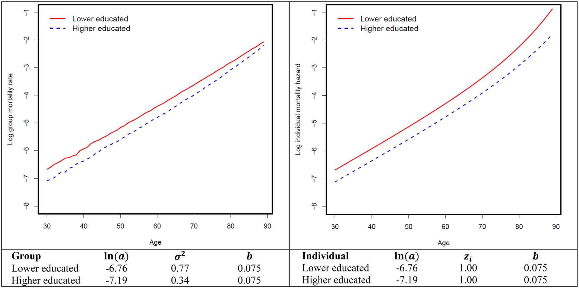
Mortality differentials between lower-educated and higher-educated groups over the life course at group and individual levels

Table 1.

Results from standard Cox model applied to simulated data

	Figure 1		Figure 2
	HR	95% CI	HR	95% CI
Higher educated, cohort 1	0.55	[0.53, 0.57]	0.55	[0.53, 0.57]
(Higher educated, cohort 1) * age groups	1.03	[1.03, 1.04]	1.03	[1.03, 1.04]
Higher educated, cohort 2			0.59	[0.57, 0.62]
(Higher educated, cohort 2) * age groups			1.02	[1.01, 1.02]
Higher educated, cohort 3			0.71	[0.68, 0.73]
(Higher educated, cohort 3) * age groups			0.98	[0.98, 0.99]
Higher educated, cohort 4			0.82	[0.78, 0.85]
(Higher educated, cohort 4) * age groups			0.95	[0.95, 0.96]

Notes:

^1.HR: Hazard Ratio; CI: Confidence Interval

^2.100,000 cases are randomly drawn from 1 million cases in each simulated data. They are split into long format by 12 five-year age groups: 30–34, 35–39, 40–44, 45–49, 50–54, 55–59, 60–64, 65–69, 70–74, 75–79, 80–84, and 85–90. These age groups are coded from 1 to 12.

^3.Time metric in continuous Cox model is attained age (age of death or being censored). Therefore, the main effects of age groups are not controlled in the model. Inclusion does not alter the results.

^4.Advantageous over other parametric models, Cox model does not need to make any parametric assumption of the underlying hazard function. Piecewise exponential model (piecewise constant hazard) and discrete time non-parametric baseline model (estimated with pgmhaz command) are also used to test the robustness of results. These two models provide almost identical results to those from Cox model. But these models do not adjust for gamma distribution of frailty.

4.1.2. Mortality patterns across birth cohorts with changing frailty variance

We then examine how mortality selection operates in the context of changing frailty variance while the individual-level hazard pattern is fixed (i.e., the true causal effect of education on mortality is fixed at the individual level). Figure 2 shows the mortality differentials between lower-educated and higher-educated groups over the life course across four birth cohorts assuming a fixed-mortality pattern at the individual level. We further let frailty variance be fixed at 0.77 across four hypothetical birth cohorts for lower-educated group, while it increases from 0.34 to 1.50 for the higher-educated group. The mortality curve of the higher-educated group becomes flatter at the group level, while the individual hazard curve remains unchanged. This is because when frailty variance increases, frail individuals are selected out of the population at a faster rate (Figure 3). This causes the group-level mortality curve to be quickly dominated by relatively robust members and consequently become flatter. As a result, mortality differentials between the lower- and higher-educated groups widen at the group level across four cohorts but remain fixed at the individual level. In other words, even though the true effect of education on mortality remains unchanged at the individual level, the educational mortality gap at the group level can still increase across cohorts as a result of the changing frailty variance. We further apply the standard Cox model to these simulated data and find that without purging mortality selection mechanism, the yielded changing associations between education and mortality risk over the life course reflect the group-level rather than individual-level pattern (Table 1).

Figure 2.

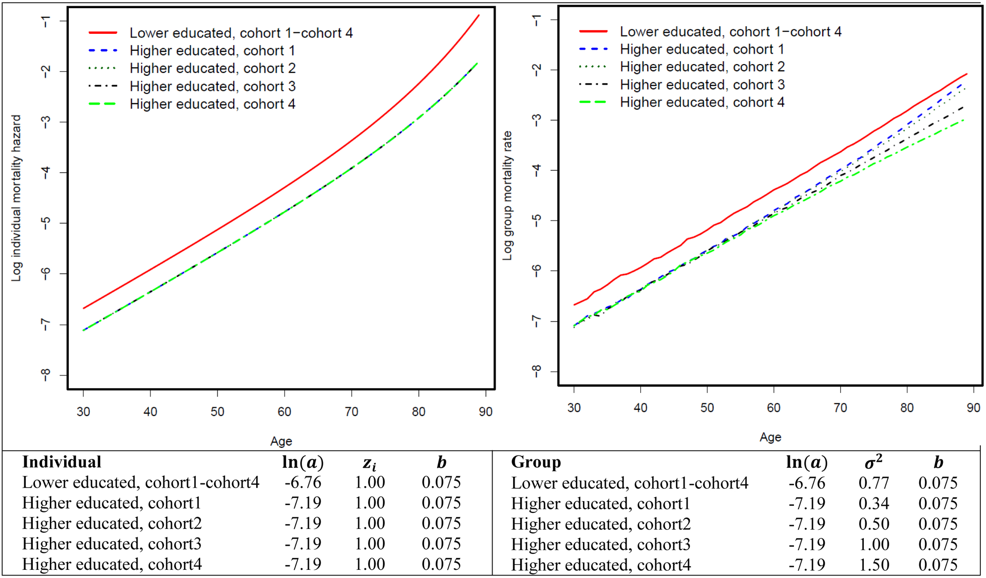
Mortality differentials between lower-educated and higher-educated groups over the life course across multiple birth cohorts assuming increasing frailty variance among the higher-educated group.

Figure 3.

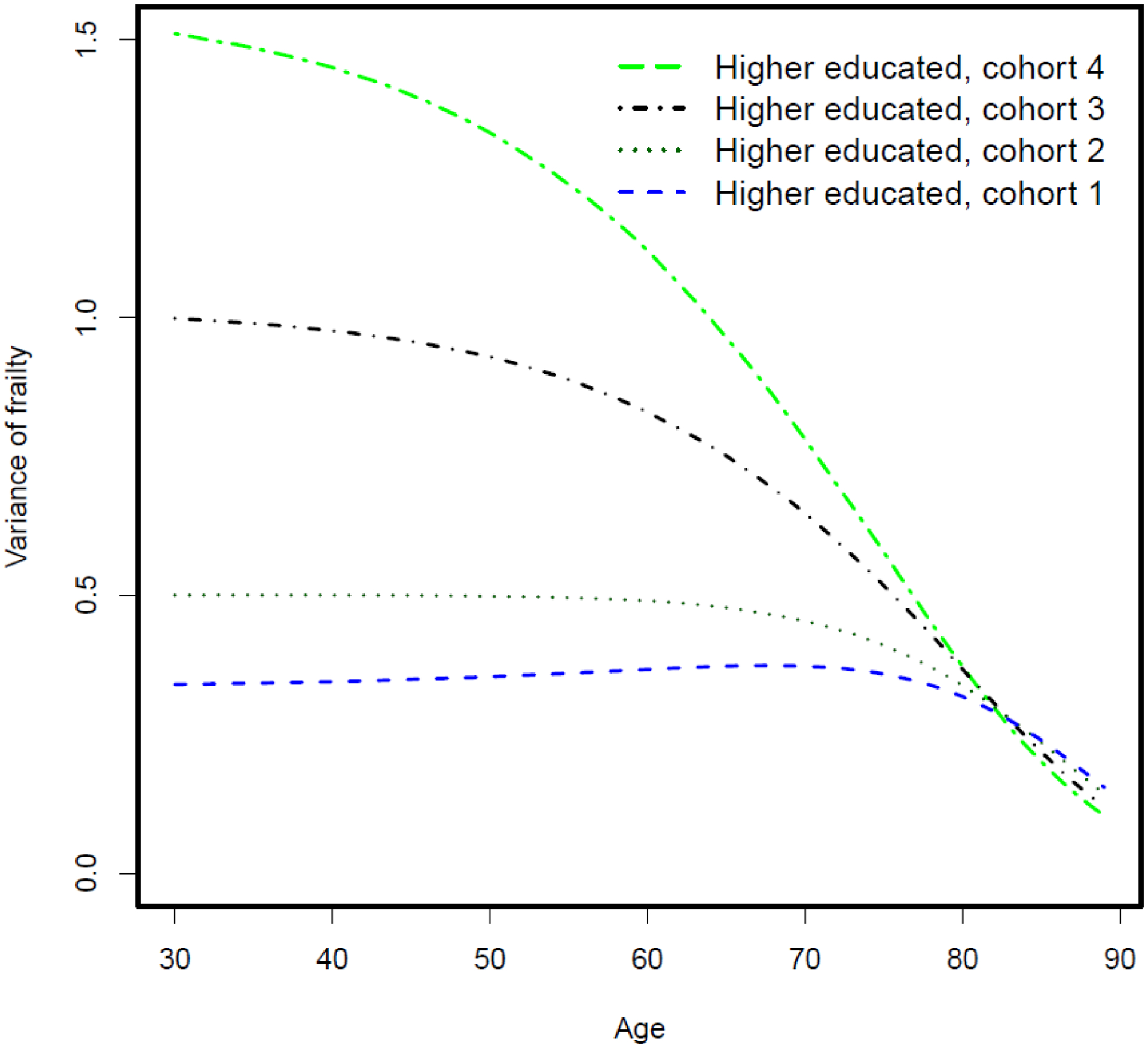
Variance of frailty over the life course among four hypothetical cohorts of higher-educated groups

Due to the flatter mortality curve at the group level, the corresponding life expectancy at age 30 increases from 50.35 years to 52.50 years across these four hypothetical cohorts with increasing frailty variance among higher-educated groups. This, in turn, leads to a widening gap in life expectancy between lower- and higher-educated groups across cohorts as shown in Figure 4, even though the extent of survival advantage associated with higher education remains unchanged at the individual level.

Figure 4.

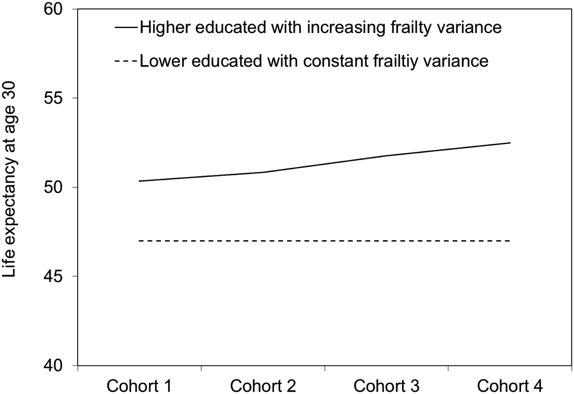
Gaps in life expectancy at age 30 between lower-educated and higher-educated groups across four hypothetical cohorts assuming increasing frailty variance among the higher-educated group

Next, we conduct a simulation experiment in which the frailty variance decreases among the lower-educated group (Appendix Figure A–3, Figure A–4, and Figure A–5). We let the individual-level hazard pattern be fixed or the true effect of education on mortality be fixed at the individual level. We further fix the frailty variance across three hypothetical birth cohorts for the higher-educated group and let it decrease for the lower-educated groups. When variance of frailty distribution decreases across birth cohorts for lower-educated groups, the mortality curve becomes steeper at the group level. As a result, mortality differentials between lower- and higher-educated groups widen and life expectancy gap increases across these three hypothetical cohorts.

4.2. Empirical evaluation

4.2.1. Counterfactual simulation analysis

How does mortality selection work in the real world? A major challenge to the empirical investigation of cohort changes and mortality selection is that the true distribution of frailty is unobserved in the population. However, since our main focus is the change between cohorts and education differences in the relative magnitude of frailty variation (rather than the variances of the absolute scores of unobserved frailty), it is possible to construct a proxy indicator of relative frailty variances through longitudinal survey data. We rely on PSID data to construct this frailty indicator for individuals and sub-populations before they reach age 17, after which some of them will be in college. We calculate a health problem summary index by adding up the number of health problems from a 12-item list before the person reaches age 17. The variance of this index is then used as a proxy for the unobserved frailty variance.⁵

We calculate the variance measure for high school or less and any college and for the 1950, 1960, 1970, and 1980 cohorts respectively. We also adjust the individual-level index for the differences in the mean of this index across cohort-education subgroups, so that the cohort changes in frailty variance is purged of any changes in their means. We then express the calculated frailty variance, for the college and non-college groups as a percentage of the frailty variance in their respective 1950 cohorts. This gives us the relative sizes of frailty variance. For example, if the frailty variance in cohort 1950 and cohort 1960 are ${\sigma }_{1950}^2$ and ${\sigma }_{1960}^2$ respectively, then the relative percentage for cohort 1960 is calculated as: $\frac{{\sigma }_{1960}^2}{{\sigma }_{1950}^2}.$

Figure 5 reports the calculated absolute frailty variance and relative frailty variance using this method. The left panel shows the absolute frailty variance. Different from the simulations for the 1990 synthetic birth cohort, the any college has a larger frailty variance than non-college across all four birth cohorts, which is partially due to lower means among this group. This implies that the age-dependent mortality pattern between these two groups will be similar to that of the higher-educated cohort 4 vs. lower-educated in Figure 2. That is, the any college group will have a flatter slope than non-college group. The right panel shows relative frailty variance declines across cohorts for both education groups, but the decline is more dramatic in relative terms for the lower-educated group. This pattern is consistent with our prediction that the changing family background composition in different education groups may interact with the macro process of improving health capital and cause the variance of frailty distribution to decrease at a faster rate among the lower-educated group than the higher-educated group. This implies that mortality curves will become steeper for both education groups across four birth cohorts but the change is greater for those without a college education, which may then widen the mortality gap between these two education groups across birth cohorts. For sensitivity analysis, we also created a similar health index from NHANES 1999–2012. Appendix Figure A–7 shows the cross-cohort pattern is similar to the one in Figure 5.

Figure 5.

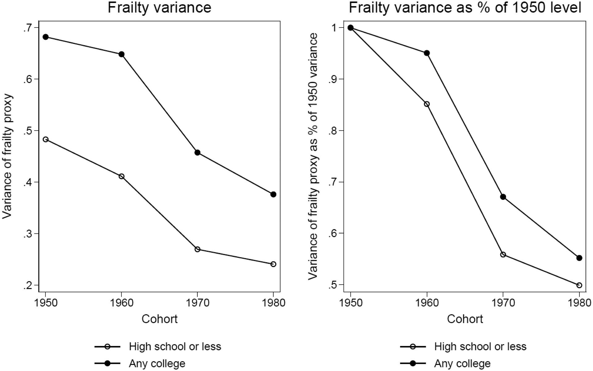
Absolute frailty variance and relative frailty variance as a percentage of the 1950 level for high school or less and any college groups from PSID 1968–2013

Notes: Data are from PSID 1968–2013. Sample consists of all individuals born from 1950–1989 who had information on early life disease measures before age 17. Sample size for these four cohorts is 11,394.

We follow the counterfactual simulation procedure explained in the method section to estimate the contribution of mortality selection to the widening educational health disparities from the 1950s to 1960s cohorts.

Step (1): We generate logged age-dependent mortality rates for the two education groups in the 1950s and 1960s birth cohorts from NHIS data. Following the Gompertz function of age-dependent mortality pattern, we use a linear function of log mortality rate to extrapolate mortality rates up to age 90 as shown in Figure 6. As predicted from the frailty variance in Figure 5, any college has a flatter slope than high school or less for both birth cohorts. However, the 1960s birth cohorts have flatter slopes than those from the 1950s despite a smaller variance of frailty, which is probably due to period-related medical advancement in older ages. Based on these age-specific mortality rates, we construct life tables and generate life expectancies at age 30 as shown in the top panel of Table 2. Life expectancies for high school or less and any college increase by 1.50 and 2.56 years across the two birth cohorts, respectively. Therefore, the gap between the two education groups increases from 5.70 to 6.76 years, which indicates a difference of 1.06 years between the two birth cohorts.

Figure 6.

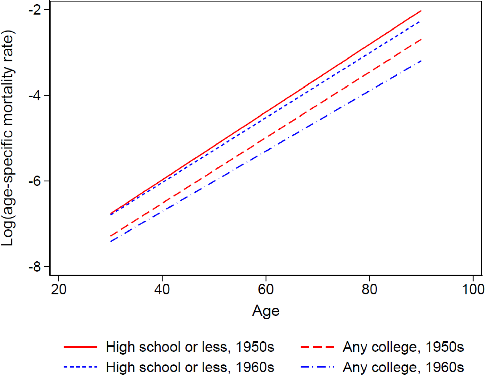
Observed and extrapolated mortality patterns for two education groups in the 1950s and 1960s birth cohorts from NHIS 1986–2009 with linked mortality through 2011

Notes: Data are from NHIS 1986–2009 surveys linked to mortality data through 2011. Sample size for the 1950s and 1960s birth cohorts is 575,705 experiencing 23,665 deaths and 8,509,452 person-years of exposure. Following the Gompertz function of age-dependent mortality pattern, we use a linear function of log mortality rate to extrapolate mortality rates up to age 90.

Table 2.

Life expectancies at age 30 in high school or less and any college groups in the 1950s and 1960s birth cohorts from empirical and simulated data using PSID frailty measure

	High school or less	Any college
	Empirical		C-H
Cohort 1950s	47.02	52.72	5.70
Cohort 1960s	48.52	55.28	6.76
1960s-1950s	1.50	2.56	1.06
	Simulated (mortality selection present)		C-H
Cohort 1950s	46.65	52.38	5.73
Cohort 1960s	46.68	53.37	6.69
1960s-1950s	0.03	0.99	0.96
	Simulated (mortality selection absent)		C-H
Cohort 1950s	46.65	52.38	5.73
Cohort 1960s	46.98	53.43	6.46
1960s-1950s	0.33	1.05	0.72

Notes: Empirical data are from NHIS 1986–2009 surveys linked to mortality data through 2011. The sample size for the 1950s and 1960s birth cohorts is 575,705 experiencing 23,665 deaths and 8,509,452 person-years of exposure. Following the Gompertz function of age-dependent mortality pattern, we use a linear function of log mortality rate to extrapolate mortality rates up to age 90. Based on these observed and extrapolated mortality rates, we construct life tables and calculate the life expectancies at age 30.

Step (2): We calibrate the frailty variance for the two education groups in the 1950s cohort so that the predicted age-dependent mortality rates can replicate those observed in the NHIS. By following the calibration method, we are able to generate simulated 1950s mortality patterns very similar to those created from the NHIS data as shown in Figure 7 when b = 0.075, σ² = 0.63 and 0.87 for high school or less and any college, respectively. Therefore, we decide to use these numbers as the variance of frailty for these two education groups in the 1950s cohort.

Figure 7.

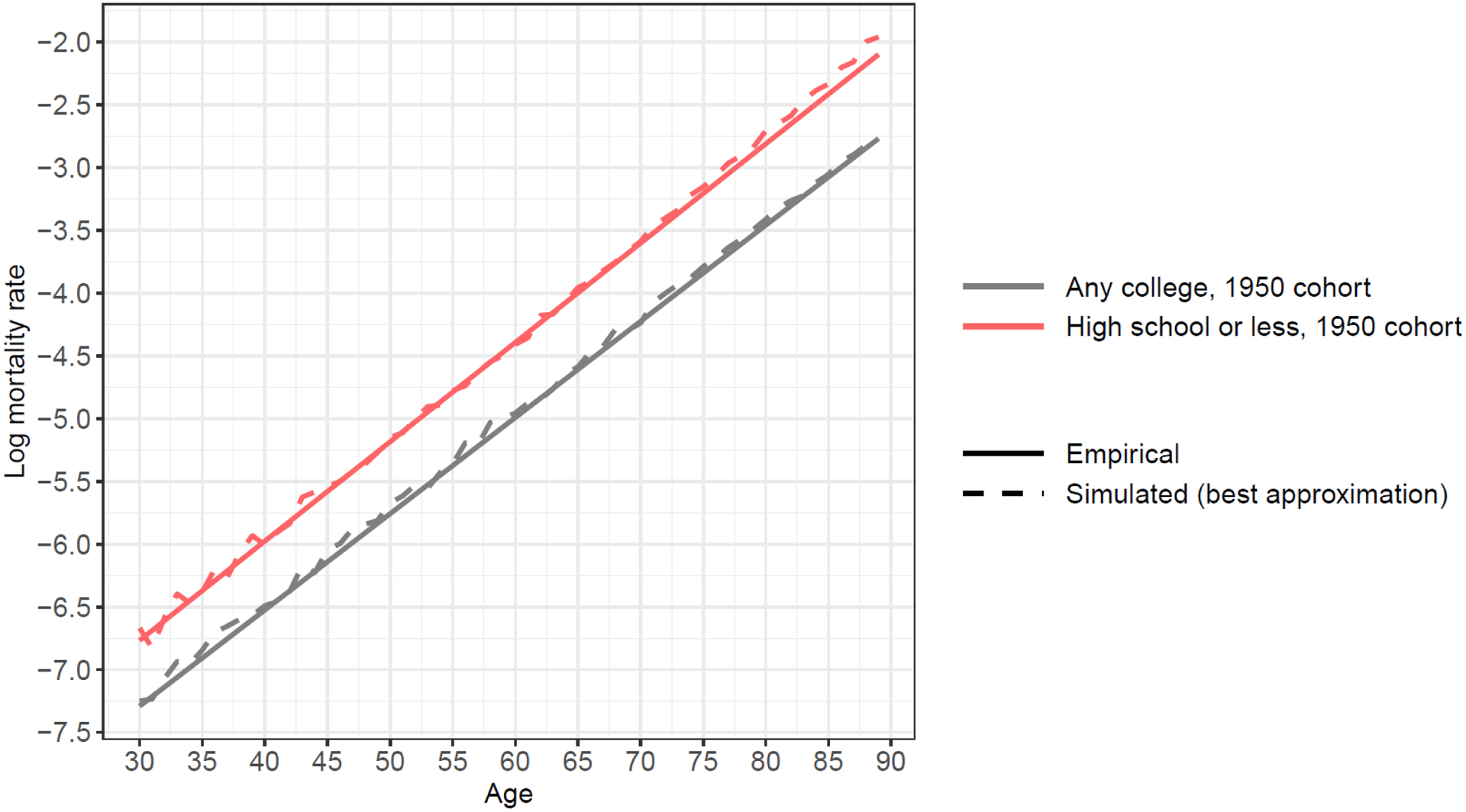
A comparison between a simulated mortality pattern using variance of frailty from calibration and an observed mortality pattern from NHIS data, 1950s birth cohort

Notes: Empirical data are from NHIS 1986–2009 surveys linked to mortality data through 2011. Sample size for the 1950s birth cohort is 320,173 experiencing 17,728 deaths and 5,093,549 person-years of exposure. Following the Gompertz function of age-dependent mortality pattern, we use a linear function of log mortality rate to extrapolate mortality rates up to age 90.

Step (3): We obtain frailty variances for the later birth cohorts based on their relative percentages as calculated from PSID data. We use the calibrated variances from Step 2 as the 1950 cohorts’ baseline in deriving the 1960 cohorts’ frailty variance, which is 0.54 for high school or less and 0.83 for any college. Note that the larger frailty variance in the any college group is inconsequential for our analysis because only the relative percentage to the 1950 cohorts within each education group is used for the simulation.

Then we follow steps (4) to (7) laid out in the methods section and find life expectancy gap between these two education groups increases by 0.96 years from the 1950s to 1960s cohort when mortality selection mechanism is present (as shown in the middle panel of Table 2) and increases by 0.72 years when mortality selection is absent (as shown in the bottom panel of Table 2). This means mortality selection contributes to 24% of the increase in the educational life expectancy gap across these two birth cohorts. Multiplying this percentage with the observed widening gap 1.06 years obtained from Step 1, we get 0.26. This means mortality selection adds 0.26 years to the observed widening educational gap in life expectancy. After adjusting for the effect of mortality selection, the cross-cohort increase in the educational life expectancy gap still exists but is now 0.8 year.

4.2.2. Sensitivity analysis with different data and model specifications

We replicate this counterfactual analysis using relative frailty variance information obtained from NHANES data and find that mortality selection contributes to 21% of the increase in the educational life expectancy gap from the 1950s to the 1960s cohorts, which translates to 0.22 years (Appendix Table A–2). In other words, the gap would have increased by 0.84 years (1.06–0.22=0.84) if mortality selection were not in effect; this estimate is very similar to the PSID results. We further do a sensitivity analysis using Gamma-Gompertz model specification (Appendix 2 and Appendix Table A–1) and find the contribution of mortality selection is around 17%.

5. Discussions and Conclusions

In demographic research, cohort changes in age-specific mortality rates and life expectancy are important indicators of the cohort changes in health conditions and between-group disparities. However, the presence of unobserved frailty and mortality selection mechanisms may lead to cohort changes in these population-level indicators even when there are no actual cohort changes in the individual mortality patterns. Therefore, empirical estimates of cohort changes in health disparities and life expectancy may be biased if we do not adjust for the mortality selection mechanism. We examined the impact of mortality selection in simulated as well as real data.

In the simulation experiments, we find (1) trends in life expectancy across birth cohorts can be altered by the variance of frailty distribution in the absence of change in the level and shape of individual mortality curve; and (2) trends in disparities in health and life expectancy between more- and less-educated groups across birth cohorts may be distorted by the changes in the variance of frailty distribution in the absence of change in the health (mortality) difference at the individual level (i.e., in the absence of change in the true causal effect of education at the individual level). For example, if variance of frailty distribution increases among the more-educated group or decreases among the less-educated group, disparities in health and life expectancy widen across birth cohorts. If frailty variance decreases among the more-educated group or increases among the less-educated group, disparities in health and life expectancy narrow across birth cohorts. These simulation experiments demonstrate the complexity of the ways in which changing unobserved frailty distributions may contribute to the observed patterns in health disparities between lower- and higher-educated groups across cohorts.

We then demonstrate the relevance of the mortality selection mechanism to empirical research using the counterfactual simulation method. We create two scenarios—one with mortality selection in effect, the other a counterfactual scenario without mortality selection. By comparing the different amounts of growth in the life expectancy gap in these two scenarios, we find that mortality selection contributes to 21–24% of the widening life expectancy gap between the high school or less and any college groups from the 1950s to 1960s birth cohorts. We also use a different model specification (Gamma-Gompertz) and find the contribution of mortality selection is slightly lower, which is 17%. We further use a different categorization of education (college degree or more vs. without college degree) and the results suggest that the contribution of mortality selection is about 20%.

A major challenge to the empirical evaluation of the mortality selection effect is that true frailty distribution is not observed. We use the summary disease index before age 17 from PSID and NHANES as a proxy for frailty. We are not particularly concerned about the elevated frailty variance among the higher-educated group for three reasons. First, the frailty variance here is the coefficient of relative variation, which is the variance divided by mean, to account for changing means across birth cohorts. The reason why frailty variance is higher among the higher-educated group is partially because their means are lower. Second, the information we used in the counterfactual simulation is not the raw frailty variance but the cohort changes in relative magnitude of frailty variation. That is the percentage of the frailty variance in later birth cohorts to their respective 1950s cohort within each educational group. This percentage is not affected by the between-educational group difference in frailty variance. Third, the empirical age-dependent mortality patterns by education for the 1950s birth cohort are consistent with the larger frailty variance among the higher-educated group, which has a flatter slope of mortality acceleration compared to the lower-educated group.

This study faces several limitations. First, better frailty measures should be collected in the future in order to more robustly and accurately estimate the contribution of mortality selection to the trends in health disparities. We have considered several other possible proxies for frailty, e.g., birth weight, parental health, Apgar scores. For the purposes of this study, we need to construct the frailty variance by education and cohort. But these proxies are either not available for early birth cohorts or do not have information on level of education. Second, even though the rule governing the contribution of mortality selection to cohort trend in life expectancy gap is applied to all the model specifications, the estimate of exact contribution does depend on model specification. Our analysis implies a range of 17%−24%. This is a common problem in the unobserved frailty literature (Keiding et al. 1997; Heckman and Singer 1982). Bound analysis using different model specifications might be one way to account for this uncertainty. Due to these limitations, we should interpret the empirical findings with caution. The exact contribution of mortality selection to the widening educational life expectancy gap from the 1950s to the 1960s cohort is very hard to be accurately estimated because of the unobservability nature of frailty. The goal of this paper is to illustrate how mortality selection may complicate the interpretation of cohort trend in health disparities and life expectancy gap, and propose a counterfactual simulation procedure to tentatively estimate this contribution. The exact contribution, however, does need future research to further push this endeavor forward with better knowledge and measures of frailty when they become available.

Notwithstanding these limitations, this study demonstrates that mortality selection can complicate the cohort trend in health disparities and life expectancy. We caution that population health scientists need to carefully consider the impact of composition changes on the trends in health disparities and life expectancy across cohorts. Other work has pointed out that it is not easy to completely and accurately solve the mortality selection bias even if we know the underlying individual-level hazard function and group-level frailty distribution function (Heckman and Singer 1982; Keiding et al. 1997; Hougaard et al. 1994). Recent methodological developments suggest using an appropriately weighted survival curve (Cole and Hernan 2004; Hernan 2010) or accelerated-failure-time model (Bradburn et al. 2003) to mitigate mortality selection bias. These strategies for addressing changing mortality selection across birth cohorts is worth further examination. The counterfactual simulation procedure we propose in this article can be utilized as an alternative to these methods to mitigate or estimate the mortality selection effect.

Appendix

Appendix 1. Basic mathematical formulation for simulation

We start our simulation by setting up a model for individual hazard function. Following Vaupel et al. (1979), we let individuals in a cohort differ from each other in the value of frailty (denoted as z) characterizing their susceptibility to death, such that the force of mortality conditional on z is

$${\mu }_i\left(x\right)=z_i{\mu }_0\left(x\right)$$ (1)

where μ_i (x) is the force of mortality for individual i at age x, z_i is frailty for individual i at the initial age, and μ₀ (x) is the unobserved baseline hazard function with frailty of 1. An individual with a frailty of 1 can be called a “standard” individual. An individual with frailty of 1.5 is one and half times more likely to die at any particular age than the standard individual. An individual with a frailty of 0.5 is only half as likely to die. Frailty z_i follows a Gamma distribution at the initial age, with p.d.f.:

$$f_0\left(z\right)={\lambda }^k{z}^{k-1}{e}^{-\lambda z}/\Gamma \left(k\right)$$ (2)

where λ and k are the parameters of the distribution. The mean and variance of a Gamma variable are given by:

$$\overline{z}=k/\lambda$$ (3a)

$${\sigma }^2=k/{\lambda }^2$$ (3b)

We follow earlier work to set mean frailty $\overline{z}$ as 1 (which is also the value of frailty for a “standard” individual). Thus, the shape parameter k equals λ, and the variance of frailty distribution σ² equals the inverse of k.

The mortality selection mechanism yields a cohort-level force of mortality $\overline{\mu }\left(x\right)$ as

$$\overline{\mu }\left(x\right)=\frac{{\mu }_0\left(x\right)}{1+{\sigma }^{2}H\left(x\right)},$$ (4)

where the cumulative hazard function from initial age to age x is $H\left(x\right)={\int }_0^x{\mu }_0\left(t\right)dt$ (Vaupel et al. 1979). From comparing formula (2) and (4), we see that cohort mortality function $\overline{\mu }\left(x\right)$ deviates from individual hazard function μ₀ (x). The higher value of the variance of frailty distribution σ², the more the slope of $\overline{\mu }\left(x\right)$ deviates from that of μ₀ (x); the deviation also increases with age as H(x) is an increasing function of x (Yashin et al. 2002).

The theory of population heterogeneity posits that death selectively removes the frailest members of a cohort so that the mortality rate at cohort level becomes increasingly dominated by robust members over the life course (Vaupel et al. 1979; Vaupel and Yashin 1985a). This means that the individual hazard curve should be steeper than the cohort mortality curve, or individuals “age” faster than heterogeneous cohorts (Vaupel and Yashin 1985b). This conclusion is also inferred from formula (4). Cohort mortality function $\overline{\mu }\left(x\right)$ in discrete time is observed and is often parameterized as a Gompertz function (Gompertz 1825). Gavrilov and Gavrilova (2011) use data for single-year birth cohorts with hazard rates measured at narrow (monthly) age intervals and find mortality trajectory at advanced ages follows the Gompertz law up to the ages 102–105 years without a noticeable deceleration. Yashin and Iachine (1997) infer the underlying individual hazard function from the semiparametric shared-frailty model using Danish twins’ data, and findings support the assumption that individuals age faster than cohorts. Their findings imply that individual hazard curve is steeper than Gompertz.

Since there are limited empirical data to support any conjecture about individual hazard curve, some studies have assumed individual hazard curve as a Gompertz function in human populations (Service 2000; Wrigley-Field 2014). The model can be specified as:

$${\mu }_0\left(x\right)=a{e}^{bx},$$ (5)

where a is the hazard at initial age and b is the rate of mortality acceleration. Replacing μ₀ (x) in formula (1) with formula (5), we get the force of mortality for individual i at age x

$${\mu }_i(x)=z_{i}a{e}^{b}x,$$ (6a)

or the logarithm form:

$$\text{ln}\left({\mu }_i\left(x\right)\right)=\text{ln}\left(a\right)+bx+\text{ln}\left(z_i\right).$$ (6b)

The rate of increase in mortality rate at age x is the derivative of ln(μ_i (x)) at age x, i.e., $\frac{d\text{ ln}\left({\mu }_i\left(x\right)\right)}{dx}=b$. In other words, individual log mortality curve is a linear function of x with fixed slope b. However, by assuming individual hazard function as formula (6a) or (6b), the simulated cohort mortality curve will “age” even slower than Gompertz. Our simulations based on this Gompertz specification, presented in Appendix Table A–1 and Appendix Figure A–1 as Model specification A, are also consistent with this view.

Instead, Vaupel and Yashin (1985b) showed that the individual mortality curve can be specified in a different way so that the population-level mortality curve closely approximates the empirical pattern. Following their formulation with some modifications, we assume individual baseline hazard function as

$${\mu }_0\left(x\right)={\mathit{\text{ae}}}^{bx}{e}^{\frac{a\left(e^{bx}-1\right)}{b}},$$ (7)

⁶ where the force of mortality for individual i at age x is

$${\mu }_i\left(x\right)=z_{i}a{e}^{\left(bx\right)}{e}^{\frac{a\left(e^{bx}-1\right)}{b}},$$ (8a)

or

$$\text{ln}\left({\mu }_i\left(x\right)\right)=\text{ln}\left(a\right)+bx+\frac{a\left(e^{bx}-1\right)}{b}+\text{ln}\left(z_i\right).$$ (8b)

The rate of increase in mortality rate at age x is the derivative of ln(μ_i (x)) at age x, i.e., $\frac{d\text{ ln}\left({\mu }_i\left(x\right)\right)}{dx}=b+a{e}^{bx}$. In other words, the rate of individual mortality acceleration is a Gompertz function of age x; it increases as age increases. More importantly, by assuming individual hazard function as formula (8a) or (8b), the simulated cohort mortality curve will follow a Gompertz function $\overline{\mu }\left(x\right)=a{e}^{\beta x}$ or $\text{ln}\left(\overline{\mu }\left(x\right)\right)=\text{ln}\left(a\right)+\beta x$, which is consistent with empirical pattern (Gompertz 1825; Gavrilov and Gavrilova 2011). The group-level rate of mortality acceleration is β. Our simulations based on this specification, presented in Appendix Table A–1 and Appendix Figure A–1 as Model specification B, are also consistent with this view.

We follow Vaupel and Yashin (1985b) in specifying the frailty distribution as a Gamma distribution, but alternative distributions, namely Weibull and Lognormal distributions, are used in robustness checks and presented in Appendix 2, Appendix Table A–1 and Appendix Figure A–1. Specifying the frailty distribution as Gamma and Weibull distribution both provide reasonably good approximation of cohort mortality curve. We keep with previous literature such as work by Vaupel and Yashin in using the Gamma distribution, and the results are similar under a Weibull distribution (see Appendix Figure A–1). Overall, no matter which individual hazard function or frailty distribution function is used, the negative association between variance of frailty and cohort slope of mortality acceleration is observed in all the model specifications.

Appendix 2. Robustness checks for alternative specifications of mortality

In this appendix, we examine the robustness of our results with respect to alternative specifications of (1) the functional form of the individual-level force of mortality and (2) the distribution of frailty in the population. The exact parametric forms, in themselves, are unobserved and therefore cannot be directly tested. Therefore, previous literature (e.g., Vaupel and Yashin 1985a, 1985b) has typically relied on the implied cohort-level age-specific mortality rates as a benchmark for selecting the proper form of these individual-level parameters. This literature suggests that to fit the observed empirical pattern of cohort mortality rate, which follows a Gompertz curve, the individual mortality hazard is best specified as the form of : ${\mu }_i\left(x\right)=z_{i}a{e}^{\left(bx\right)}{e}^{\frac{a\left(e^{bx}-1\right)}{b}}$, and the frailty distribution in the population is best fitted as a gamma distribution (see Vaupel and Yashin 1985b).

In our main simulations, we follow this literature closely in selecting our preferred model specifications for individual mortality hazard and frailty distribution. In addition, alternative specifications are examined as robustness checks. These alternative specifications are presented in Appendix Table A–1 and resulting logged cohort mortality curves are given in Appendix Figure A–1. The first row of Appendix Figure A–1 presents simulation results for logged cohort mortality in which the functional form of individual mortality hazard is changed to a Gompertz curve: μ_i (x) = z_iae^(bx), and we vary the functional form and variances of the frailty distribution. We fix the mean frailty at one unit in all these simulations. In the second row of this figure, we keep the individual mortality hazard as specified in our main simulations, and the frailty distribution is altered in the same way as it is in the first row. Vaupel and Yashin (1985b) also listed examples of other functional forms of individual mortality hazard, but as their mathematical derivation shows, other functional forms do not generate an increasing cohort mortality rate over age and are therefore omitted in our analysis.

Our additional simulation results yield four conclusions that all support our choice of model specifications in our main simulations. First, although a natural choice for the functional form of mortality pattern is to choose a Gompertz mortality curve at the individual level, we and many prior studies found that, if the individual-level mortality hazard is specified as Gompertz, the implied cohort mortality pattern will not follow the observed Gompertz curve after age 70 or 80. Although literature has debated whether the deceleration of cohort mortality curve in late age is real, more refined analysis finds that cohort mortality trajectory at advanced ages follows the Gompertz law up to the ages 102–105 years without a noticeable deceleration (Gavrilov and Gavrilova 2011). Second, in our specification in the main simulation analysis, as well as in Vaupel and Yashin’s original specifications, the individual-level mortality hazard curve that takes the form of ${\mu }_i\left(x\right)=z_{i}a{e}^{\left(bx\right)}{e}^{\frac{a\left(e^{bx}-1\right)}{b}}$ generates a Gompertz pattern on the cohort level, which closely approximates the empirical pattern. Third, specifying the frailty distribution as Gamma and Weibull distribution both provide reasonably good approximation of cohort mortality curve. We keep with previous literature such as work by Vaupel and Yashin in using the Gamma distribution, and the results are similar under a Weibull distribution. Fourth, even though alternative specifications generate different shapes of the cohort mortality curve, it is reassuring to see, from comparing the curves within each sub-plot of Appendix Figure A–1, that our main conclusion—that the cohort mortality increases at a faster rate over age when the variance of frailty is smaller—holds throughout all specifications.

Appendix Table A-1.

Alternative specifications with different frailty distributions and different functional forms of the individual-level force of mortality

	Frailty Distribution
	Gamma	Weibull	Lognormal
Model Specification A: individual-level force of mortality μi (x) = ziae(bx)
	σ2 = 1	σ2 = 1	σ2 = 1
Frailty Variance	σ2 = 0.75	σ2 = 0.75	σ2 = 0.75
	σ2 = 0.5	σ2 = 0.5	σ2 = 0.5
Model Specification B: individual-level force of mortality ${\mu }_i\left(x\right)=z_{i}a{e}^{\left(bx\right)}{e}^{\frac{a\left(e^{bx}-1\right)}{b}}$
	σ2 = 1	σ2 = 1	σ2 = 1
Frailty Variance	σ2 = 0.75	σ2 = 0.75	σ2 = 0.75
	σ2 = 0.5	σ2 = 0.5	σ2 = 0.5

Appendix Table A-2.

Life expectancies at age 30 in high school or less and any college groups in the 1950s and 1960s birth cohorts from empirical and simulated data using NHANES frailty measure

	High school or less	Any college
	Empirical		C-H
Cohort 1950s	47.02	52.72	5.70
Cohort 1960s	48.52	55.28	6.76
1960s-1950s	1.50	2.56	1.06
	Simulated (mortality selection present)		C-H
Cohort 1950s	46.65	52.38	5.73
Cohort 1960s	46.74	53.39	6.65
1960s-1950s	0.09	1.00	0.92
	Simulated (mortality selection absent)		C-H
Cohort 1950s	46.65	52.38	5.73
Cohort 1960s	46.98	53.43	6.46
1960s-1950s	0.33	1.05	0.72

Notes: Empirical data are from NHIS 1986–2009 surveys linked to mortality data through 2011. Sample size for the 1950s and 1960s birth cohorts is 575,705 experiencing 23,665 deaths and 8,509,452 person-years of exposure. Following the Gompertz function of age-dependent mortality pattern, we use a linear function of log mortality rate to extrapolate mortality rates up to age 90. Based on these observed and extrapolated mortality rates, we construct life tables and calculate life expectancies at age 30.

Appendix Figure A-1.

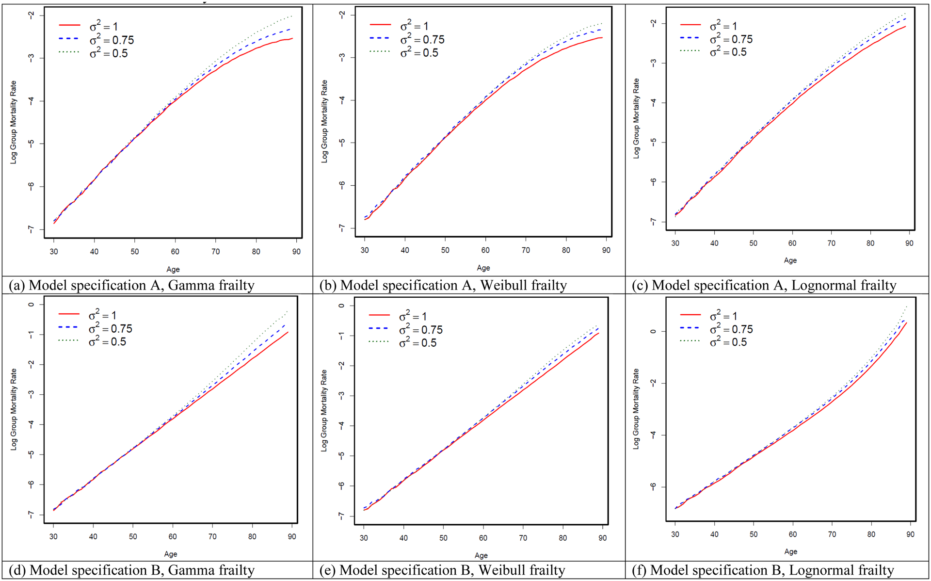
Simulation results for alternative specifications with different frailty distributions and different functional forms of the individual-level force of mortality

Appendix Figure A-2.

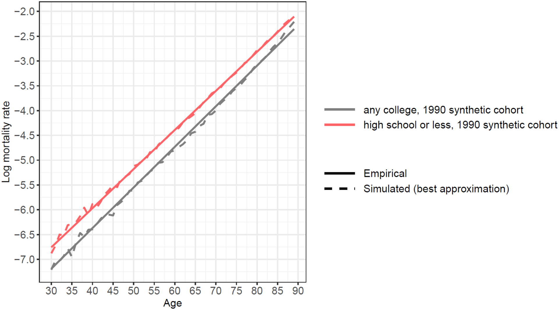
A comparison between a simulated mortality pattern using variance of frailty from calibration and an observed mortality pattern from NHIS data, 1990 synthetic birth cohort

Notes: Empirical data are from NHIS 1986–2009 surveys linked to mortality data through 2011. Sample size for the 1990 synthetic birth cohort is 253,367 experiencing 2,599 deaths in 1990. Following the Gompertz function of age-dependent mortality pattern, we fit a linear function of log mortality rate to smooth the trend.

Appendix Figure A-3.

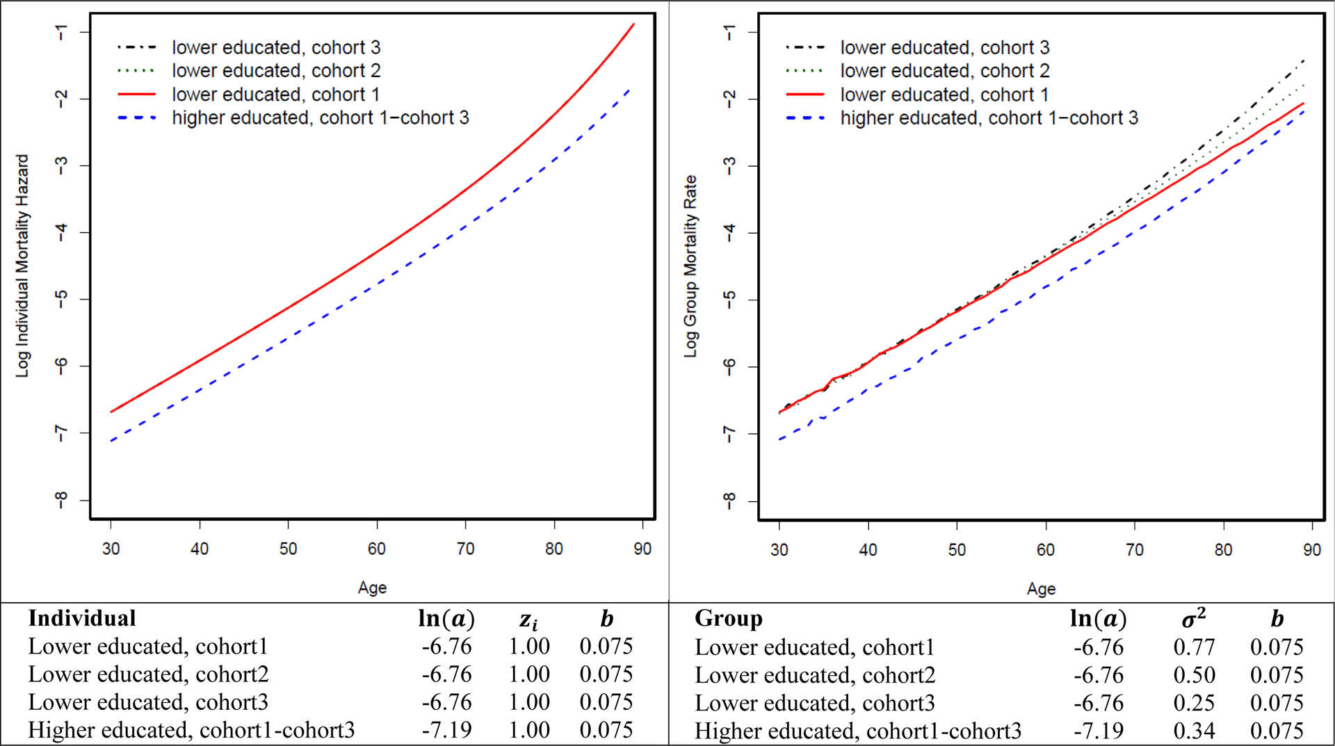
Mortality differentials between lower-educated and higher-educated groups over the life course across multiple birth cohorts assuming decreasing frailty variance among the lower-educated group

Appendix Figure A-4.

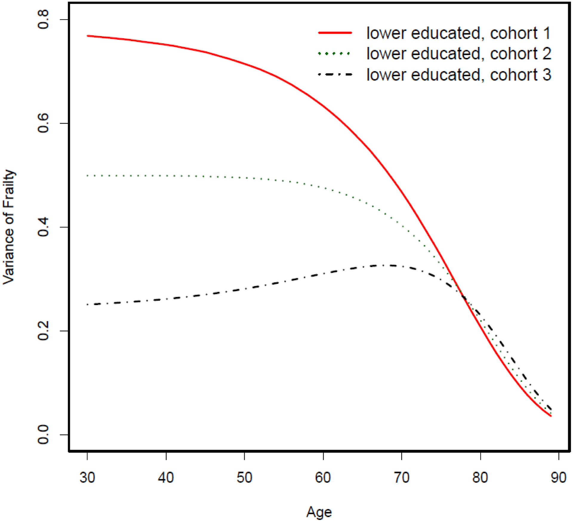
Variance of frailty over the life course among three hypothetical cohorts of the lower-educated group

Appendix Figure A-5.

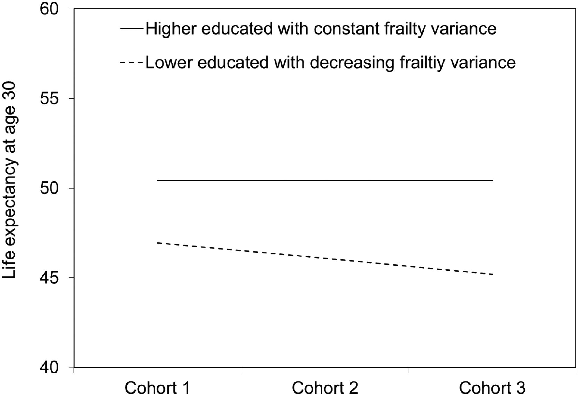
Gaps in life expectancy at age 30 between lower-educated and higher-educated groups across three hypothetical cohorts assuming decreasing frailty variance among the lower-educated group

Appendix Figure A-6.

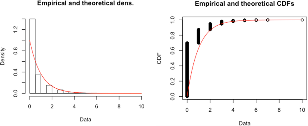
Empirical (histogram) and Theoretical (Gamma Distribution, red smooth line) Distributions of the Frailty Measure Constructed from PSID Data

To examine the distributional properties of our constructed frailty measure, we fit a Gamma distribution to the empirical distribution of our PSID-based frailty measure and compare them. The theoretical Gamma density is fitted using maximum likelihood estimation. The left panel of the figure compares the empirical and theoretical density functions, and the right panel of the figure compares the two cumulative distribution functions (CDF). The two panels suggest that the empirical distribution of our constructed frailty measure can be reasonably approximated by the Gamma distribution. In sum, while there is no perfect measure for the frailty distribution in the population, the distributional properties of our frailty measure seem to be generally consistent with our assumption of the Gamma distribution in the simulation models.

Appendix Figure A-7.

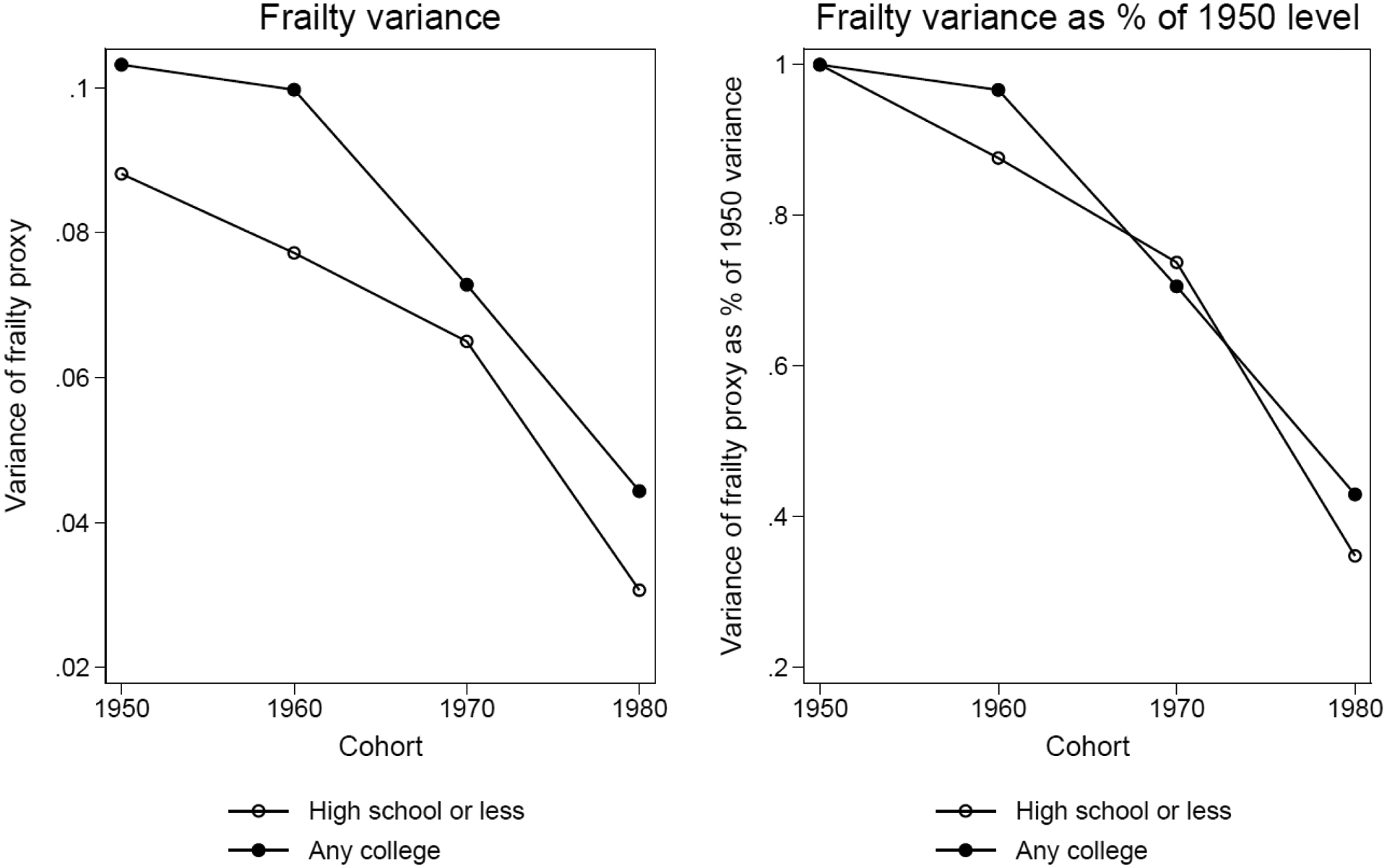
Absolute frailty variance and relative frailty variance as a percentage of the 1950 level for high school or less and any college groups from NHANES 1999–2012

Notes: Data are from NHANES 1999–2012. Sample consists of all individuals born from 1950–1989 who had information on early life disease measures before age 17. Sample size for these four cohorts is 22,181.

References

- Blewett LA, Drew JAR, Griffin R, King ML, and Williams KCW (2018). IPUMS Health Surveys: National Health Interview Survey, Version 6.3 [dataset]. Minneapolis, MN: IPUMS. [Google Scholar]
- Bradburn MJ, Clark TG, Love SB, and Altman DG (2003). Survival analysis part II: Multivariate data analysis - an introduction to concepts and methods. British Journal of Cancer 89(3): 431–436. [DOI] [PMC free article] [PubMed] [Google Scholar]
- Case A, and Deaton A (2015). Rising morbidity and mortality in midlife among white non-Hispanic Americans in the 21st century. Proceedings of the National Academy of Sciences 112(49): 15078–15083. [DOI] [PMC free article] [PubMed] [Google Scholar]
- Cole SR, and Hernán MA (2004). Adjusted survival curves with inverse probability weights. Computer Methods and Programs in Biomedicine 75(1): 45–49. [DOI] [PubMed] [Google Scholar]
- Crimmins EM, and Saito Y (2001). Trends in Healthy Life Expectancy in the United States, 1970–1990: Gender, Racial, and Educational Differences. Social Science and Medicine 52: 1629–1641. [DOI] [PubMed] [Google Scholar]
- Dannefer D (2003). Cumulative advantage/disadvantage and the life course: cross-fertilizing age and social science theory. The Journals of Gerontology: Social Sciences 58B(6): S327–S337. [DOI] [PubMed] [Google Scholar]
- Dowd JB, and Hamoudi A (2014). Is life expectancy really falling for groups of low socioeconomic status? Lagged selection bias and artefactual trends in mortality.” International Journal of Epidemiology 43(4): 983–988. [DOI] [PubMed] [Google Scholar]
- Dupre ME (2007). Educational differences in age-related patterns of disease: reconsidering the cumulative disadvantage and age-as-leveler hypotheses. Journal of Health and Social Behavior 48(1): 1–15. [DOI] [PubMed] [Google Scholar]
- Eberstein IW, Nam CB, and Heyman KM (2008). Causes of death and mortality crossovers by race. Biodemography and Social Biology 54(2): 214–228. [DOI] [PubMed] [Google Scholar]
- Feldman JJ, Makuc DM, Kleinman JC, and Cornoni-Huntley J (1989). National Trends in Educational Differences in Mortality. American Journal of Epidemiology 129(5): 919–933. [DOI] [PubMed] [Google Scholar]
- Finch CE, and Crimmins EM (2004). Inflammatory exposure and historical changes in human life-spans. Science 305: 1736–1739. [DOI] [PubMed] [Google Scholar]
- Fogel RW, and Costa DL (1997). A theory of technophysio evolution, with some implications for forecasting population, health care costs, and pension costs. Demography 34: 49–66. [PubMed] [Google Scholar]
- Gavrilov LA, and Gavrilova NS (2011). Mortality measurement at advanced ages: A study of the social security administration death master file. North American Actuarial Journal 15(3): 432–447. [DOI] [PMC free article] [PubMed] [Google Scholar]
- Goesling B (2007). The Rising Significance of Education for Health? Social Forces 85(4): 1621–1644. [Google Scholar]
- Gompertz B (1825). On the nature of the function expressive of the law of human mortality. Philosophical Transactions 27:252–253. [Google Scholar]
- Heckman JJ, and Singer B (1982). The identification problem in econometric models for duration data. In Hildebrand W (Ed.), Advances in Econometrics (pp. 1203–1213). Cambridge: Cambridge University Press. [Google Scholar]
- Hendi AS (2015). Trends in U.S. life expectancy gradients: the role of changing educational composition. International Journal of Epidemiology 44(3): 946–955. [DOI] [PMC free article] [PubMed] [Google Scholar]
- Hendi AS (2017). Trends in education-specific life expectancy, data quality, and shifting education distributions: A note on recent research. Demography 54(3): 1203–1213. [DOI] [PMC free article] [PubMed] [Google Scholar]
- Hernán MA (2010). The hazards of hazard ratios. Epidemiology 21(1): 13–15. [DOI] [PMC free article] [PubMed] [Google Scholar]
- Hougaard P, Myglegaard P, and Borch-Johnsen K (1994). Heterogeneity models of disease susceptibility, with application to diabetic nephropathy. Biometrics 50(4): 1178–1188. [PubMed] [Google Scholar]
- House JS, Lepkowski JM, Kinney AM, Mero RP, Kessler RC, and Herzog AR (1994). The social stratification of aging and health. Journal of Health and Social Behavior 35: 213–234. [PubMed] [Google Scholar]
- Hummer RA, Rogers RG, and Eberstein IW (1998). Sociodemographic Approaches to Differentials in Adult Mortality: A Review of Analytic Approaches. Population and Development Review 24(3): 553–578. [Google Scholar]
- Jemal A, Ward E, Anderson RN, Murray T, and Thun MJ (2008). Widening of Socioeconomic Inequalities in U.S. Death Rates, 1993–2001. PLOS ONE 3(5): e2181. [DOI] [PMC free article] [PubMed] [Google Scholar]
- Keiding N, Andersen PK, and Klein JP (1997). The role of frailty models and accelerated failure time models in describing heterogeneity due to omitted covariates. Statistics in Medicine 16(1–3): 215–224. [DOI] [PubMed] [Google Scholar]
- Kindig DA, and Cheng ER (2013). Even as mortality fell in most US counties, female mortality nonetheless rose in 42.8 percent of counties from 1992 to 2006. Health Affairs 32(3): 451–458. [DOI] [PubMed] [Google Scholar]
- Lauderdale DS (2001). Education and survival: Birth cohort, period, and age effects. Demography 38(4): 551–561. [DOI] [PubMed] [Google Scholar]
- Liu H, and Hummer RA (2008). Are Educational Differences in U.S. Self-Rated Health Increasing? An Examination by Gender and Race. Social Science and Medicine 67: 1898–1906. [DOI] [PMC free article] [PubMed] [Google Scholar]
- Lynch SM (2003). Cohort and life-course patterns in the relationship between education and health: A hierarchical approach. Demography 40(2): 309–331. [DOI] [PubMed] [Google Scholar]
- Lynch SM, Brown JS, and Harmsen KG (2003). Black-White differences in mortality compression and deceleration and the mortality crossover reconsidered. Research on Aging 25(5): 456–483. [Google Scholar]
- Masters RK, Hummer RA, and Powers DA (2012). Educational differences in U.S. adult mortality: a cohort perspective. American Sociological Review 77(4): 548–572. [DOI] [PMC free article] [PubMed] [Google Scholar]
- Meara ER, Richards S, and Cutler DM (2008). The gap gets bigger: changes in mortality and life expectancy, by education, 1981–2000. Health Affairs 27(2): 350–360. [DOI] [PMC free article] [PubMed] [Google Scholar]
- Montez JK, and Zajacova A (2013). Explaining the widening education gap in mortality among U.S. white women. Journal of Health and Social Behavior 54(2): 166–182. [DOI] [PMC free article] [PubMed] [Google Scholar]
- Olshansky SJ, Antonucci T, Berkman L, Binstock RH, Boersch-Supan A, Cacioppo JT, et al. (2012). Differences in life expectancy due to race and educational differences are widening, and many may not catch up. Health Affairs 31(8): 1803–1813. [DOI] [PubMed] [Google Scholar]
- Pappas G, Queen S, Hadden W, and Fisher G (1993). The Increasing Disparity in Mortality between Socioeconomic Groups in the United States, 1960 and 1986. New England Journal of Medicine 329: 103–115. [DOI] [PubMed] [Google Scholar]
- Preston SH, and Elo IT (1995). Are Educational Differentials in Adult Mortality Increasing in the United States? Journal of Aging and Health 7(4): 476–496. [DOI] [PubMed] [Google Scholar]
- Preston S, Heuveline P, and Guillot M (2001). Demography: Measuring and Modeling Population Processes. Malden, MA: Blackwell. [Google Scholar]
- Ross CE, and Wu C (1996). Education, Age, and the Cumulative Advantage in Health. Journal of Health and Social Behavior 37: 104–120. [PubMed] [Google Scholar]
- Sasson Isaac. (2016). Trends in Life Expectancy and Lifespan Variation by Educational Attainment: United States, 1990–2010. Demography 53: 269–293. [DOI] [PMC free article] [PubMed] [Google Scholar]
- Schoeni RF, Martin LG, Andreski P, and Freedman VA (2005). Persistent and Growing Socioeconomic Disparities in Disability Among the Elderly: 1982–2002. American Journal of Public Health 95(11): 2065–2070. [DOI] [PMC free article] [PubMed] [Google Scholar]
- Service PM (2000). Heterogeneity in individual mortality risk and its importance for evolutionary studies of senescence. The American Naturalist 156(1): 1–13. [DOI] [PubMed] [Google Scholar]
- Torche F (2011). “Is a college degree still the great equalizer? Intergenerational mobility across levels of schooling in the United States.” American Journal of Sociology 117(3): 763–807. [Google Scholar]
- Vaupel JW (1997). Trajectories in mortality in advanced ages. In Wachter KW, and Finch CE (Eds.), Between Zeus and the Salmon: The Biodemography of Longevity (pp. 17–37). Washington, DC: National Academy Press. [PubMed] [Google Scholar]
- Vaupel JW (2010). The theory of heterogeneity: A concise primer. Manuscript. Max Planck Institute for Demographic Research; Rostock, Germany. [Google Scholar]
- Vaupel JW, Manton KG, and Stallard E (1979). The impact of heterogeneity in individual frailty on the dynamics of mortality. Demography 16(3): 439–454. [PubMed] [Google Scholar]
- Vaupel JW, and Missov T (2014). Unobserved population heterogeneity: A review of formal relationships. Demographic Research 31: 659–686. [Google Scholar]
- Vaupel JW, and Yashin AI (1985a). Heterogeneity’s ruses: Some surprising effects of selection on population dynamics. The American Statistician 39(3): 176–185. [PubMed] [Google Scholar]
- Vaupel JW, and Yashin AI (1985b). The deviant dynamics of death in heterogeneous populations. Sociological Methodology 15: 179–211. [Google Scholar]
- Vaupel JW, and Yashin AI (1987). Repeated resuscitation: How lifesaving alters life tables. Demography 24(1): 123–135. [PubMed] [Google Scholar]
- Wrigley-Field E (2014). Mortality deceleration and mortality selection: three unexpected implications of a simple model. Demography 51(1): 51–71. [DOI] [PMC free article] [PubMed] [Google Scholar]
- Yashin AI, and Iachine IA (1997). How frailty models can be used for evaluating longevity limits: taking advantage of an interdisciplinary approach. Demography 34(1): 31–48. [PubMed] [Google Scholar]
- Yashin AI, Ukraintseva SV, Boiko SI, and Arbeev KG (2002). Individual aging and mortality rate: How are they related? Biodemography and Social Biology 49(3–4): 206–217. [DOI] [PubMed] [Google Scholar]
- Zajacova A, Goldman N, and Rodríguez G (2009). Unobserved heterogeneity can confound the effect of education on mortality. Mathematical Population Studies 16(2): 153–173. [DOI] [PMC free article] [PubMed] [Google Scholar]
- Zheng H (2014). Aging in the context of cohort evolution and mortality selection. Demography 51(4): 1295–1317. [DOI] [PMC free article] [PubMed] [Google Scholar]
- Zheng H and Cheng S (2018). A Simulation Study of the Role of Cohort Forces in Mortality Patterns. Biodemography and Social Biology 64 (3–4): 216–236. [DOI] [PMC free article] [PubMed] [Google Scholar]
- Zheng H, Yang CY, and Land KC (2016). Age-Specific Variation in Adult Mortality Rates in Developed Countries. Population Research and Policy Review 35: 49–71. [DOI] [PMC free article] [PubMed] [Google Scholar]