Clonal fitness inferred from timeseries modeling of single cell cancer genomes

Abstract

Progress in defining genomic fitness landscapes in cancer, especially those defined by copy number alterations (CNA), has been impeded by lack of time series single cell sampling of polyclonal populations and temporal statistical models^1–7. Here, we generated 42,000 genomes from multi-year time series single cell whole genome sequencing (scWGS) of breast epithelium and primary triple negative breast cancer (TNBC) patient derived xenografts (PDX), revealing the nature of CNA defined clonal fitness dynamics induced by TP53 mutation and cisplatin chemotherapy. Using a new Wright-Fisher population genetics model^8,9 to infer clonal fitness, we found that TP53 mutation alters the fitness landscape, reproducibly distributing fitness over a larger number of clones associated with distinct CNAs. Furthermore, in TP53 mutant TNBC PDX models, inferred fitness coefficients from CNA-based genotypes accurately forecast experimentally enforced clonal competition dynamics. Drug treatment in three long-term serially passaged TNBC PDX resulted in cisplatin resistant clones emerging from low fitness phylogenetic lineages in the untreated setting. Conversely, high fitness clones from treatment naive controls were eradicated, signaling an inversion of the fitness landscape. Finally, upon release of drug selective pressure dynamics were reversed, indicating a fitness cost of treatment resistance. Taken together, our findings define clonal fitness linked to both CNA and therapeutic resistance in polyclonal tumours.

Quantifying cellular fitness and its causal mechanisms in heterogeneous, polyclonal cancer cell populations remain as open problems, impeding progress in developing effective and durable therapeutic strategies^1–7. Despite well documented genomic plasticity in tumours, the question of how copy number alterations (CNA)-induced changes in the genome architecture drive etiologic and drug resistance¹⁰ processes remains understudied^11–13. The cancer field has generally lacked serial measurements from patient derived tissues to directly observe cancer evolution over realistic timescales with single cell resolution^{1,2,4,14–21}. This has hindered thorough investigation of causal factors driving selection, successfully achieved in other biological systems²². Here we use single genome-derived CNAs as clone-defining heritable genotypes to establish quantitative fitness attributes that serve as predictive measures of polyclonal growth potential. Our work has implications in at least three areas: predicting evolution in cancer; understanding how genomic instability processes leading to CNAs confer fitness; and parsing long term kinetics of drug resistance in polyclonal cancer cell populations.

Modeling clonal fitness and selection

We developed an experimental and computational platform consisting of three components: timeseries sampling and single cell whole genome sequencing of immortal cell lines and patient derived xenografts (Extended Data Fig. 1a,b); scalable phylogenetics for single cell genomes (sitka²³, Extended Data Fig. 1c); and a population genetics inspired (Wright-Fisher diffusion process) model of fitness (fitClone, Extended Data Fig. 1d,e, Supplementary Table 1). Using observed longitudinal clonal abundance measurements as input, fitClone simultaneously estimates growth trajectories, Z_i and fitness coefficients, s_i for each Clone i in the population. The model can be used to forecast evolutionary trajectories, and its posterior probability densities can reflect evidence of positive selection in polyclonal systems. Details of fitClone including theoretical assumptions and limitations of the model are discussed in the Supplementary Information.

CNAs and fitness in p53 deficient cells

We first applied the framework to immortalized 184hTERT diploid breast epithelial cell lines²⁴ in order to measure clone specific fitness associated with TP53 loss of function. Known to be permissive of genomic instability, p53 mutations are often acquired early in breast cancer evolution^4,25,26 and result in alteration of the CNA genome structure^5,6,21,24,27. We contrasted 4 timeseries samples of wildtype (p53^wt) cells (60 passages over 300 days) with two isogenic null (p53^−/−) parallel branches (p53^−/−a and p53^−/−b)²⁸, each passaged over 60 generations (285 and 220 days, respectively), and sampled 7 times. A median of 1,231 cells per passage were whole genome sequenced yielding a total of 2713, 3264, and 4881 genomes for each timeseries, respectively (Supplementary Table 1). For each of p53^wt, p53^−/−a, p53^−/−b, we inferred CNA profiles, constructed phylogenetic trees to establish clonal lineages (Methods) and measured clonal abundances over time. Phylogenetic analysis (sitka, Extended Data Fig. 2a,b) and modeling of abundances with fitClone (Extended Data Fig. 2c, Supplementary Tables 2 and 3) revealed p53^wt clonal trajectories consistent with small differences in selection coefficients amongst three major Clones E (chromosome 11q gain), D (chromosome 20 gain) and F (diploid; and used as the reference clone for fitClone modeling). In contrast, p53^−/−a showed significant expansions of clones with aneuploid genotypes (Extended Data Fig. 2d, Fig. 1a) and higher selection coefficients, where the founder diploid population was out-competed (Fig. 1b). A second independent p53 mutant timeseries p53^−/−b (Extended Data Fig. 2e–g) confirmed that CNA-bearing clones confer higher fitness. The p53 mutant lines harboured 11 (size range 47 to 1,474 cells, median 204), and 10 (size range 158 to 997 cells, median 404) distinct clones for p53^−/−a and p53^−/−b, respectively (Supplementary Table 2). Notably, selection coefficients were highest in clones with focal amplifications of known prototypic oncogenes in breast cancer^6,7,25,26(Extended Data Fig. 2d,e), in some cases on a whole genome doubled background. Clone A, the highest fitness clone in p53^−/−a (57% of cells at last timepoint, 1 + s = 1.05 ± 0.09) exhibited whole genome doubling and harboured a focal, high level amplification at the MDM4 (1q) locus (Extended Data Fig. 2d). Clone G (27% of cells at last timepoint, 1 + s = 1.03 ± 0.03), the next highest fitness clone in p53^−/−a remained diploid, with the exception of a focal high level amplification precisely at the MYC locus (8q) (Extended Data Fig. 2d). By contrast Clone K, here chosen as the reference clone for modeling, remained entirely diploid and exhibited a monotonically decreasing trajectory (from 90% to 0% of cells over the timeseries, Fig. 1b). In p53^−/−b, two clones exhibited large positive selection coefficients (Extended Data Fig. 2f,g): Clone D (52% of cells at last timepoint, 1 + s = 1.05 ± 0.02) harboured a 20q single copy gain with an additional high level amplification at the TSHZ2 locus; and Clone E (35% of cells at the last timepoint, 1 + s = 1.05 ± 0.04) harboured a chromosome 4 loss, 19p gain/19q loss and 20q single copy gain (Extended Data Fig. 2e). As seen in p53^−/−a, the ‘root’ Clone I that remained diploid was systematically out-competed, diminishing from 68% to 0% abundance over the timeseries (Extended Data Fig. 2g).

Figure 1.

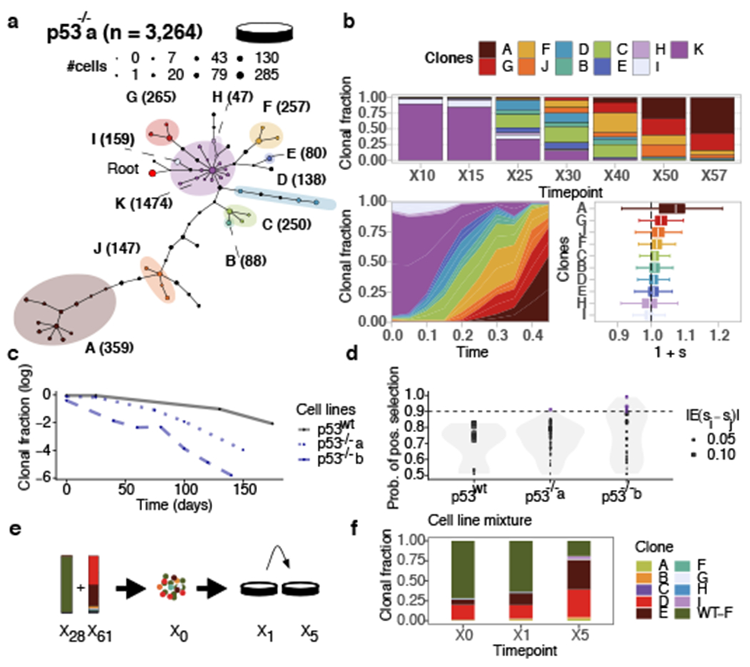
Replicate branch of p53 mutant cells and engineered mixture experiment. a) Phylogeny of 3,264 p53^−/−a cells, grouped in 11 phylogenetic clades over the timeseries where nodes are groups of cells (scaled in size by number) with shared copy number genotype and edges represent distinct genomic breakpoints. Shaded areas represent clones. Tree root is denoted by the red circle. b) Observed clonal fractions over time, inferred trajectories and quantiles of the posterior distributions over selection coefficients of fitClone model fits to p53^−/−a with respect to the reference Clone K. In the box plots, the white line represents the median of the distribution, box edges show 1.5× the interquartile range and whiskers extend to 25th and 75th percentiles. c) Clonal fraction of the diploid reference over time. d) Distribution over the probability of positive selection (PPS) over pairs of clones computed as max(P(s_i > S_j), 1 – P(s_i > s_j)). Purple dots denote PPS over 0.9. e) Mixture experiment of 75% TP53^wt (timepoint X28) and 25% TP53^−/−b (timepoint X61). f) Observed clonal fractions in the mixture series with diploid, p53^wt shown as (WT-F).

Relative to p53^wt, rates of expansion of both p53^−/−a and p53^−/−b aneuploid clones were significantly higher, leading to rapid depletion of diploid cells (Fig. 1c, p = 6.72e − 04). Copy number breakpoints per cell increased as a function of fitness and were higher in the p53 mutant lines, however point mutation rate remained comparatively stable (Extended Data Fig. 2h,i). In addition, both p53 mutant lines exhibited higher posterior probability of positive selection (clone pairs with probability >0.9) relative to the p53^wt setting (Fig. 1d). Accordingly, we sought to experimentally confirm clonal fitness in p53 mutant cells associated with increased aneuploidy. We challenged higher fitness aneuploid clones (D and E, which dominated by X60) from p53^−/−b with p53^wt diploid populations in de novo population mixtures and collected samples over 5 generations in culture (Fig. 1e). scWGS sequencing of the mixture samples revealed Clones D and E to monotonically increasing from 18% and 7% to 35% and 37% of the population by passage 5, while the diploid p53 wildtype cells were out-competed, decreasing from 75% to 19% at final passage (Fig. 1f). Thus, the enforced competition resulted in re-emergence of p53 mutant aneuploid clones and relative depletion of diploid cells, supporting the original fitClone model fits. Together, these results show a broader clone fitness landscape, with overall higher fitness of clones harbouring whole genome, chromosomal and segmental aneuploidies arising in p53 mutant cells (Extended Data Fig. 2d,e). Notably, high fitness clones featured high level amplification of proto-oncogenes often seen in human breast cancer (e.g., MDM4, MYC, TSHZ2), suggesting that p53 loss is permissive of fitness-enhancing CNAs with etiologic roles in cancer⁷.

Modeling fitness in human breast cancer

We next studied timeseries CNA clonal expansions of p53 mutant primary human breast cancers from four PDX transplant series. We generated serial scWGS samples from one Her2 positive (HER2+SA532) and three TNBC (TNBC-SA609, TNBC-SA1035, TNBC-SA535), sampled over 927, 619, 381 and 353 days, respectively (Extended Data Fig. 3) yielding a median of 303 high quality genomes per sample (9,970 total) for downstream analysis (Supplementary Table 1). All series exhibited progressively higher tumour growth rates over time (Extended Data Fig. 3b–d) and maintained hormone receptor status from early to late passages (Supplementary Tables 4 and 5). Bulk WGS and scWGS confirmed all four tumours harboured TP53 mutations with bi-allelic and truncal distribution across clones (Supplementary Table 6). Resulting phylogenetic analysis indicated all PDX were polyclonal at the CNA level (Fig. 2, Extended Data Fig. 4a–i), with in cis gene expression impacts inferred from single cell RNA-seq data derived from the same single cell suspensions (Supplementary Table 7, Methods).

Figure 2.

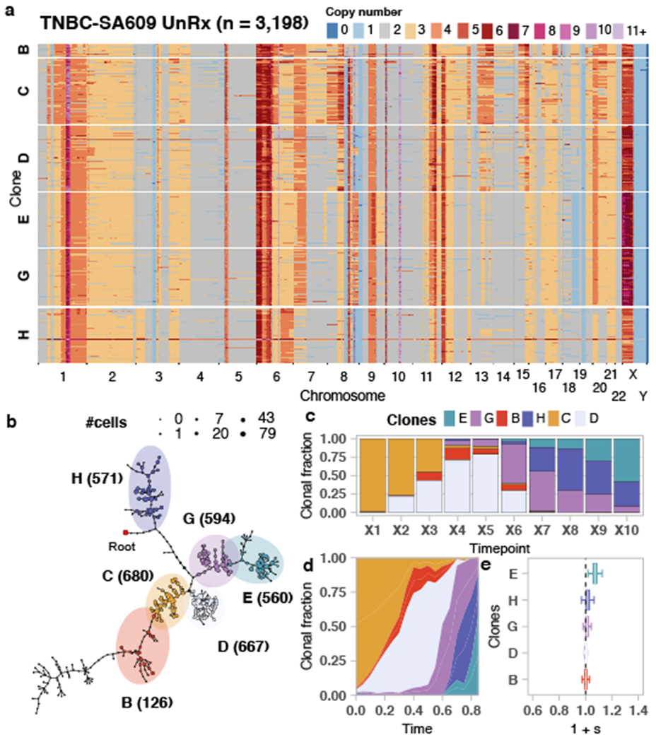
Fitness landscapes of untreated TNBC-SA609 UnRx PDX. a) Heatmap representation of copy number profiles of 3,198 cells from TNBC-SA609, grouped in 6 phylogenetic clades. b) Phylogeny for TNBC-SA609. c) observed clonal fractions, d) inferred fitClone trajectories and e) quantiles of the selection coefficients with respect to the reference Clone C. Boxplots are as defined in Fig. 1b.

In contrast with HER2+SA532, all TNBC PDX models exhibited evidence of clonal dynamics and variation in selection coefficients consistent with positive selection and differential fitness (Fig. 3a). For TNBC-SA1035, 11 clones were detected (Extended Data Figs. 4a,b and 5); the reference Clone A had initial prevalence of 20% but was not detectable by the last timepoint. Clone E, expanding to 69% at passage X8 from minor prevalence at the initial timepoint (1 + s = 1.06 ± 0.03) (Extended Data Fig. 4c,d, Supplementary Table 3), formed a distinct clade, distinguished by a hemizygous deletion of the centromeric locus of 8p, an extra copy gain of the telomeric end of 11q and a focal gain of 19q12 harbouring the CCNE1 locus (Extended Data Figs. 4a and 5a). In TNBC-SA535, three of ten clones propagated after the initial timepoint (Extended Data Fig. 4d–f). Clone G, characterized by loss of chromosome X, exhibited expansion from minor prevalence at passage X5 to 76% at passage X9 (1 + s = 1.02 ± 0.01, Extended Data Fig. 4f). For TNBC-SA609 Line 1, six clones were observed (Fig. 2a,b). Clones E (1 + s = 1.07 ± 0.02) and H (1 + s = 1.02 ± 0.02) had the highest selection coefficients, exhibiting growth from undetectable levels to 59% and 32% respectively by timepoint X10. Clone C contracted from near 100% at the initial timepoint to undetectable levels by X10 (Fig. 2c–e). Growth of Clones E (Extended Data Fig. 6a) , G, and H and contraction of Clone C (Extended Data Fig. 6b) was observed reproducibly in replicate transplants (Extended Data Fig. 6c–e). Notably, clones in the HER2+ series exhibited a maximum probability of positive selection of 0.67 suggesting overall clonal selection close to neutral (Extended Data Fig. 4i). In contrast, in all 3 TNBC series at least one clone showed probability of positive selection > 0.9 (Fig. 3a).

Figure 3.

Positive selection in TNBC PDX untreated. a) Distribution over the PPS over pairs of clones, analogous to Fig. 1d. b) Clonal proportions of TNBC-SA609 Line 1 at X3 and X8 used to generate the initial mixture M0 and subsequent serial passaging, yielding 4 samples. c) Forward simulations from the original timeseries and starting population proportions in the initial experimental mixture a. Simulated trajectories are shown superimposed with mean simulation (red line) and observed clonal fractions (blue dots). The observation time is adjusted to match the simulation diffusion time.

Forecasting clonal trajectories

Next, we experimentally validated the fitness coefficients as indicators of positive or negative selection. We carried out forward simulations from fitClone using selection coefficients estimated from the original timeseries, and compared these with serially passaged physical clonal mixtures of late (X8) and early (X3) timepoints from TNBC-SA609 (Line 1). Two mixture-retransplant-serial-passage experiments were conducted with different initial starting conditions (Fig. 3b, Extended Data Fig. 7a). Clone E was forecast to fixate with highest probability (0.39) in the first, and Clones E and H were forecast with high probability of fixation in the second (0.14 and 0.04, respectively) (Fig. 3c, Extended Data Fig. 7b). The two series were then sequenced with scWGS, yielding 6,453 and 6,730 genomes respectively. In the first mixture (Extended Data Fig. 7c), six clones from the original timeseries were recovered with between 26 to 767 (median 155) cells. As anticipated by the model, Clone E emerged as a high fitness clone (1 + s = 1.08 ± 0.03), and by the last timepoint, Clones E and H had swept through, comprising 94% of cells. For the second mixture (Extended Data Fig. 7d), four clones (C, E, G, and H) from the original timeseries were recovered. Clone E was the only clone that increased in prevalence (from 5% to 24%) and had the highest selection coefficient (1 + s = 1.02 ± 0.03). In contrast, Clones C, G and H exhibited relatively stable prevalences (Extended Data Fig. 7d). Thus, both mixture experiments demonstrated expansion of the predicted highest fitness Clone E, even when starting from low initial proportions (2% and 5% of cells).

The fitness cost of platinum resistance

Using CNA clone specific fitness measurements, we next asked how drug treatment with cisplatin (standard therapy for primary TNBC) perturbs the fitness landscape of the three PDX series. For each timeseries, we propagated a separate branch treated with cisplatin (Extended Data Figs. 1b and 3, Methods) to induce gradual onset of platinum resistance, physically confirmed with progressive reduction in tumour growth inhibition (TGI)²⁹ (%TGI from first to last cycle: TNBC-SA609: 77% to 4.7%; TNBC-SA1035: 76% to 15%; TNBC-SA535: 58% to 16%, Extended Data Fig. 3b–d). For TNBC-SA609 a total of five independent transplant lineages were surveyed with technical replicates for Lines 1 & 2 (Methods). In each series, emergent clones on treatment were distinct in phylogenetic origin from those with high fitness in the untreated setting, indicating an inversion of the clone fitness landscapes (Fig. 4a, Extended Data Fig. 8a). Suppression of high fitness clones that dominated in the absence of treatment, and expansion of low fitness and/or previously unobserved genotypes led to a substantially altered rank order of selection coefficients in treated samples relative to untreated samples (Fig. 4b, Extended Data Fig. 8b–c). For TNBC-SA609 Line 2, growth dynamics over X3-U; X4-UT; X5-UTT; X6-UTTT; X7-UTTTT (U = no treatment timepoint, T = treated timepoint), resulted in expansion of Clone B and its derivative clones (A and R), from a starting population comprised primarily of Clones C, D and B (Extended Data Fig. 9) in three replicate transplants. Notably, resistant clones in all three replicate treated lines were phylogenetically distinct from Clone H - the highest fitness clone in the treatment-naive setting (Extended Data Fig. 8a–c left panel, Extended Data Fig. 9a,e). The other two TNBC series also supported a fitness inversion, exhibiting monotonically decreasing prevalence of treatment-naive high fitness clones, and increasing prevalence of low fitness clones. Importantly, in both TNBC-SA535 and TNBC-SA1035, both high and low fitness clones were observed in initial conditions, ruling out sampling bias as a strict determinant of selection dynamics (Extended Data Figs. 10 and 5). Specifically, low fitness clones in the untreated series all increased, with the fittest clones under no treatment decreasing to near zero prevalence (e.g., TNBC-SA535 Clone G (Extended Data Fig. 10a) ; TNBC-SA1035 Clone E). Probability of positive selection increased in the treatment series (Extended Data Fig. 8d), indicating more clones under positive selection in the cisplatin setting, and selection coefficients exhibited a wider variance between clones.

Figure 4.

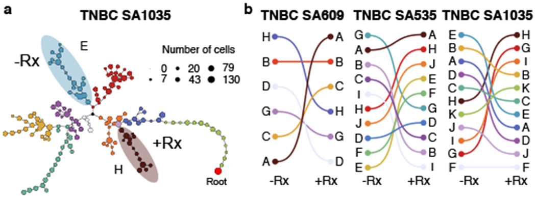
Fitness landscape reversal in early Cisplatin treatment in TNBC PDX models. a) Phylogenetic tree for the TNBC-SA1035 annotated with fittest clones in −Rx and Rx. b) Inversion of the fitness landscape. Clones are ranked according to their median selection coefficients in untreated and treated conditions, with the top-ranked clones highest.

Finally, we tested the impact of lifting the drug selective pressure at each timepoint, with drug holiday replicate transplants (Extended Data Figs. 1b and 3a–e). In TNBC-SA609, inverted fitness was reversible in a short interval (Extended Data Fig. 9). In the first drug holiday X5-UTU, clonal composition reverted to consist predominantly of precursor Clone B with 90% abundance, and only 10% abundance from Clone A (Extended Data Fig. 9c, d-Line 1, Line 3-Holiday panel,e). However, X6-UTTU and X7-UTTTU consisted of >99% Clone A, similar to their on-treatment analogues, and no reversion was detected. Thus, when clonal competition was possible in the absence of drug, cells derived from the precursor B clade outcompeted Clone A, indicating clone-specific cisplatin resistance has a fitness cost. Moreover, the specificity of reversion between X4-UT to X5-UTU reflects selection of predefined clones with differential fitness. The TNBC-SA1035 series exhibited more moderate reversibility. Clone G growth was attenuated from 10% at X5-UT to 9% at X6-UTU, compared to 20% at X6-UTT (Extended Data Fig. 5b–e). Similarly, in TNBC-SA535 (Extended Data Fig. 10c–e) growth attenuation of the highest fitness Clone A (Extended Data Fig. 10b) in the treatment setting was observed in the holiday setting, and Clone E exhibited clonal fractions similar to treated timepoints at X7-UTTU, X8-UTTU, and X9-UTTTU. However, Clone E increased to 32% in X10-UTTTTU from 10% in X9-UTTTT. Thus, in all series, treatment selective pressure was reversible with drug holidays, consistent with a fitness cost to platinum resistance.

Discussion

In population genetics, the repeated observation of dominance or decline in clones, defined here by CNA genotypes, implies that either the genotype or a factor heritably linked to the genotype (such as SNVs or epigenetic states), is a determinant of fitness. We expect additional variation due to SNVs, structural variations from genomic rearrangements, or rare CNAs beyond first approximation estimates will additively impact fitness. However, deeper population sampling would be required to appropriately capture these effects. Our results, decoded by measuring single cell timeseries, suggest that fitness linked to CNAs may be under-appreciated. This has implications for interpreting etiologic processes of tumour suppressor driven cancers, shown by inducing TP53 loss, where rates of structural variation acquisition and deviation away from diploid configurations conferred fitness advantages. Over successive generations in vitro with TP53 mutational perturbation and in three TNBC PDX in the context of cisplatin drug treatment, emergent CNA measurably contributed to the fitness landscape, consistent with a continual diversifying mechanism that induces competitive clonal advantages.

Our results demonstrate that timeseries fitness mapping is a realistic initial approach for studying how the impact of driver mutations inducing genomic instability leads to clonal expansions and evolutionary selection. The ability to genetically manipulate the systems we describe provides a future path to mechanistically dissecting fitness impacts of individual CNA regions. Furthermore, as the impact of drug intervention on CNA driven cancer evolution is a key determinant of patient outcomes across all human cancers^{20,21,30–32}, forecasting the trajectories of cancer clones is of immediate importance to understanding therapeutic response in cancer, and for deploying adaptive approaches¹⁰. We suggest the presence of resistant genotypes that have a chemotherapeutic fitness cost may define time windows within which clonal competition could be exploited. Future investigation in patients with timeseries tumour or cell-free DNA- based population genetics modeling may therefore enable evolution-informed approaches to clinical management³³.

Methods

All methods are detailed in the Supplementary Information. We studied normal human breast epithelial cells²⁴ in vitro and in breast cancer PDX, sequencing >129,500 whole genomes from single cells over interval passaging (scWGS DLP+ method²⁸ Extended Data Fig. 1a,b, Supplementary Table 1). After read-coverage based quality control and omission of replicating cells, we retained >42,000 genomes from 113 libraries across cell lines and PDX transplants for analysis (average 995,000 reads/cell, 0.022x coverage). We calculated phylogenetic trees over cells to identify genotypic clones and their relative abundances as a function of time

Human mammary cell lines and serial passaging and mixtures

The human mammary epithelial cell line 184-hTERT wild type and isogenic 184-hTERT-P53 KO cell line, generated from 184hTERT WT-L9, were grown as previously described^24,28. p53^−/− was knocked out by using CRISPR/Cas9 technology and one clone (99.25) was serially passaged to further subdivided at passage 10 into “branch a” and “branch b” parallel knockout branches (NM_000546(TP53):c.[156delA];[156delA]), p.(GIn52Hisfs*71), and the absence of TP53 protein was confirmed with western blot (Supplementary information). Two branches of 184-hTERT-p53^−/− (clone 95.22) along with the counterpart wild type branch were serially passaged over ~55-60 generations, by seeding ~1 million cells into a new 10 cm tissue culture treated dish (FalconCABD353003) and cryopreserving every fifth passage. Mammary Epithelial Cell SingleQuot Kit Supplements (MEGM™), Growth Factors (Lonza CC-4136), with 5 μg ml⁻¹ transferrin (Sigma) and 2.5 μg ml⁻¹ isoproterenol (Sigma) were used as a growth media as previously described²⁴. Cells were grown to around 85-90% confluence, trypsinized for 2 minutes (Trypsin/EDTA 0.25%,VWR CA45000-664), re-suspended in cryopreservation media (10% DMSO-Sigma-D2650, 40% FBS-GE Healthcare SH30088.03, 50% media) and frozen to −80 °C at a rate of −1 °C min⁻¹. Cells were cultured continuously from passage 10 (post initial cloning²⁴) to passage 60 for 184-hTERT WT and upto passage 57 and passage 55 for the p53^−/− branches a and b, respectively, from initial cloning/isolation. Genome sequencing was undertaken at passages 25, 30, 51 and 60 from the wild type branch, passages 10, 15, 25, 30, 40, 50 and 57 from p53^−/− branch a and passages 20, 30, 35, 40, 45, 50 and 55 from p53^−/− branch b. Also, the transcriptome sequencing was carried out on passages 11 and 57 of p53^−/− branch a and passages 15, 30 and 50 of p53^−/− branch b. All cell line cultures were tested negative for mycoplasma by ‘PCR Mycoplasma contamination detection test’. The initial conditions of the mixtures were biased in favour of diploid cell populations in a 3:1 ratio of 184-hTERT WT p28 (SA039) and p53^−/− clone 95.22 (SA906b) passage 61. Prior to plating in the culture, an aliquot was subjected to DLP+ to measure the baseline clonal composition labelled as X0, and 2,701 single cell genomes were generated. At 80% confluence on the plate, cells from X1 were harvested and serially passaged upto the 20th passage. Single cell whole genome sequencing data from three time points X0, X1 and X5 with a median of 898 cells per timepoint was collected.

Establishment and serial passaging of patient derived xenografts

The Ethics Committees at the University of British Columbia approved all the experiments using human resources. Patients in Vancouver, British Columbia were recruited, and samples were collected under the tumour tissue repository (TTR-H06- 00289) and transplanted in mice under the animal resource centre (ARC) bioethics protocol (A19-0298-A001) approved by the animal care committee (University of British Columbia BC Cancer Research Ethics Board H20-00170) protocols. After informed consent, tumour fragments from patients undergoing excision or diagnostic core biopsy were collected. Tumour materials were processed as described in³⁴ and transplanted in 8-12 weeks old, female mice approved by the animal care committee. Briefly, tumour fragments were chopped finely with scalpels and mechanically disaggregated for one minute using a Stomacher 80 Biomaster (Seward Limited, Worthing, UK) 1 ml to 2 ml cold DMEM/F-12 with Glucose, LGlutamine and HEPES (Lonza 12-719F). An aliquot of 200 μl of medium (containing cells/clumps) from the resulting suspension was used equally for 4 transplantations in mice. Tumours were transplanted subcutaneously in mice as previously described³⁴ in accordance with SOP BCCRC 009.

Serial passaging of PDX

Tumours were serially passaged as previously described³⁴. Briefly, for serial passaging of PDX, xenograft-bearing mice were euthanized when the size of the tumours approached 1000 mm³ in volume (combining together the sizes of individual tumours when more than one was present). The tumour material was excised aseptically, and processed as described for primary tumour. Briefly, the tumour was harvested and minced finely with scalpels then mechanically disaggregated for one minute using a Stomacher 80 Biomaster (Seward Limited, Worthing, UK) in 1 ml to 2 ml cold DMEM-F12 medium with Glucose, L-Glutamine and HEPES. Aliquots from the resulting suspension of cells and fragments were used for xenotransplants in the next generation of mice and cryopreserved. Serially transplanted aliquots represented approximately 0.1-0.3% of the original tumour volume. HER+SA532 and TNBC-SA609 PDX were passaged upto 10 generations and scDNAseq was carried out at each timepoint. The other three untreated and treated PDX timeseries were generated in the same way for 4-5 passages.

TNBC PDX tumour mixing experiments

Frozen vials from the untreated TNBC PDX passages three (X3) and eight (X8), were thawed and physically remixed in two different volumetric proportions of X3:X8 by tumour weight. The ratio of approximately 1:1 and 1:0.4, labelled as mixture branch a and branch b, respectively. From each of different dilutions, 200 μl of aliquot was transplanted in two mice each using the same protocol described above. Before transplantation, a small proportion of the physical mixture of cells from the 1:1 ratio, was subjected to whole genome single cell sequencing to measure the baseline clonal composition labelled as M0 and its subsequent PDX as M1. The tumour cell mixture was then serially passaged over 4 generations for branch a and 5 generations for branch b, designating the transplants as M1-M4 and M1 to M5, respectively. Tumours from serial passages (X3:X8) from both mixtures branches were collected and analysed with scWGS (DLP+) as for other samples.

TNBC PDX timeseries treatment with cisplatin

Female NRG mice of 8-12 weeks of age and genotype were used for randomized controlled transplantation treatment experiments. Drug treatment with cisplatin, an analog of platinum salts was commenced when the tumour size reached approximately 300 mm³ to 400 mm³. Cisplatin (Accord DIN: 02355183) was administered intraperitoneally (IP) at 2 mg kg⁻¹ every third day for 8 doses maximum (Q3Dx8). The dosage schedule was adjusted 50% less than what is mentioned in the literature^35,36 and around one third of the maximum tolerated dose (MTD) calculated in the immunodeficient female mice of 8-12 weeks of age (Supplementary Information). Low dose cisplatin pulse and tumour collection timings were optimized to achieve the experimental aims of tumour resistance. The aim was to collect the tumour at around 50% shrinkage (from the starting tumour at the time treatment started) in size when measured with a caliper. Cisplatin 1 mg ml⁻¹ was diluted in 0.9% NaCl to obtain concentrations 200 μl/20 g of mouse weight and kept in glass vials at room temperature. Quality control (QC) drug samples were prepared freshly on each day prior to the dosing. For all three TNBC PDX, 8 female mice at initial passage were transplanted in parallel for the treatment/treatment holiday study group. The choice of sample size was made to get atleast 3 mice in the treatment group. Half of the mice were treated with cisplatin when tumours exhibited ~ 50% shrinkage, the residual tumour was harvested as above and re-transplanted for the next passage in the group of eight mice. Again, half of the mice at X5 were randomly kept untreated while the other half were exposed to cisplatin following the same dosing strategy. Four cycles of cisplatin treatment were generated, with a parallel drug holiday group at each passage. Cisplatin treated tumours were coded as UT, UTT, UTTT, UTTTT for each of the four cycles of drug respectively, while the tumours on drug holiday were labelled as UTU, UTTU and UTTTU for the three timepoints. The number of Ts in the coded label shows the number of cycles of drug exposure. scWGS and scRNAseq was carried out on each tumour during the timeseries treatment with counterpart drug holiday and untreated controls (Extended Data Fig. 3a). In particular, TNBC-SA609 PDX was processed to establish 5 independent lines to explore the biological and technical replicate tumours as well as treatment series. All five lines from TNBC-SA609 were passaged identically after initial establishment. Line 1 untreated samples were seeded (X3 to X4) from a freshly dissociated tumour, whereas 4 other lines (all treated and Line 2 Un-treated) were seeded (X3 to X4) from a frozen vial of tumour. Technical replicates were collected and sequenced for Lines 1, 2.

PDX tumour growth measurement curves

NRG mice received sub-cutaneous (SQ) inoculation of tumour cells (150 μl) on day 0. The tumours were allowed to grow to palpable solid nodules. Around 7-9 days after they were palpable, their size was measured with calipers every 3rd day. Tumours were measured in two dimensions using a digital caliper and expressed as tumour volume in mm³; defined as: [Volume= 0.52×(Length)×(Width)×(Width)]. Record of patient derived xenografts 10 generations timeseries, HER2+SA532 and TNBC-SA609 exhibited progressively higher tumour growth rates in later passages (Extended Data Fig. 3b–d). Tumour growth inhibition (TGI) percentage range was defined as: [1 − (mean volume of treated tumours)/(mean volume of control tumours) × 100%]²⁹.

Single cell whole genome sequencing and library construction with DLP+

All libraries, including metrics on number of cells, average number of reads per cell and quality control metrics are listed in Supplementary Table 1. Tumour fragments from PDX samples were incubated with collagenase/hyaluronidase, 1:10 (10X) enzyme mix (STEM CELL technologies, Catalog #07912) in 5 ml DMEM/F-12 with Glucose, L-Glutamine and HEPES (Lonza 12-719F) and 1%BSA (Sigma) at 37 °C. Intermittent gentle pipetting up and down was done every 30 minute for 40-60 seconds, during the first hour with a wide bore pipette tip, and every 15-20 min for the second hour, followed by centrifugation (1100 rpm, 5 min) and supernatant removal. The tissue pellet was resuspended in 1 ml of 0.25 percent trypsin-EDTA (VWR CA45000-664) for 1 min, superadded by 1 ml of DNAse/dispase (100 μl/900 μl), (StemCell 07900,00082462) pipetted up and down 2 min, followed by neutralization with 2% FBS in Hanks’ Balanced Salt Solution (HBSS) with 10 mM HEPES (STEMcells Catalog #37150). Undigested tissue was removed by passing through a 70 μm filter and centrifuged for 5 min at 1100 rpm after topping it up to 5 ml with HBSS. Single cells pellet was resuspended in 0.04% BSA (Sigma) and PBS to achieve ~1 million per ml concentration of cells for robot spotting for DLP+.

Robot spotting of single cells into the nanolitre wells and library construction

DLP+ library construction was carried out as described in²⁸. Briefly, single cell suspensions from cell lines and patient derived xenografts were fluorescently stained using CellTrace CFSE (Life Technologies) and LIVE/DEAD Fixable Red Dead Cell Stain (ThermoFisher) in a PBS solution containing 0.04% BSA (Miltenyi Biotec 130-091-376) incubated at 37 °C for 20 minutes. Cells were subsequently centrifuged to remove stain, and resuspended in fresh PBS with 0.04 percent BSA. This single cell suspension was loaded into a contactless piezoelectric dispenser (sciFLEXARRAYER S3, Scienion) and spotted into the open nanowell arrays (SmartChip, TakaraBio) preprinted with unique dual index sequencing primer pairs. Occupancy and cell state were confirmed by fluorescent imaging and wells were selected for single cell CN profiling using the DLP+ method²⁸. Briefly, cell dispensing was followed by enzymatic and heat lysis. After lysis, tagmentation mix (14.335 nL TD Buffer, 3.5 nL TDE1, and 0.165 nL 10% Tween-20) in PCR water were dispensed into each well followed by incubation and neutralization. Final recovery and purification of single cell libraries was done after 8 cycles of PCR. Cleaned up pooled single-cell libraries were analyzed using the Aglient Bioanalyzer 2100 HS kit. Libraries were sequenced at UBC Biomedical Research Centre (BRC) in Vancouver, British Columbia on the Illumina NextSeq 550 (mid- or high-output, paired-end 150-bp reads), or at the GSC on Illumina HiSeq2500 (paired-end 125-bp reads) and Illumina HiSeqX (paired-end 150-bp reads). The data was then processed to a quantification and statistical analysis pipeline²⁸.

Processing of cell lines and patient derived xenografts for scRNAseq data

All libraries generated using 10x scRNAseq are listed in Supplementary Table 8. Suspensions of 184-hTERT p53^wt and KO cells were fixed with 100% ice-cold methanol prior to preparation for scRNAseq. Single cell suspensions were loaded onto the 10x Genomics single cell controller and libraries prepared according to the Chromium Single Cell 3’ Reagent Chemistry kit standard protocol. Libraries were then sequenced on an Illumina Nextseq500/550 with 42bp paired-end reads, or a HiSeq2500 v4 with 125bp paired-end reads. 10x Genomics CellRanger, V3.0.2 (V3 chemistry), was used to perform demultiplexing, alignment and counting.

Viable frozen tumour clumps and fragments were incubated with digestion enzymes as with DLP+ single cells preparation (as above) and the cells were resuspended in 0.04% BSA in PBS. Dead cells were removed using the Miltenyi MACS Dead Cell Removal kit and cells were processed as previously described³⁷. To avoid processing artifacts and dissociation methods, the timings were tightly controlled between the samples. Library construction of the samples at the same time point was performed on the same chips. Library construction sample batch groupings are listed in Supplementary Table 7.

Phylogenetic tree inference, clone determination and clonal abundance measurements

We developed a single cell Bayesian tree reconstruction method based on copy number change point binary variables called sitka²³ to fit phylogenetic trees to the copy number profiles. In the output of sitka, cells are the terminal leaf nodes of the phylogenetic topology. The inferred trees were post-processed to identify clonal populations from major clades. With clonal populations defined, their abundances were counted as a function of timeseries and these were used for fitness inference (see below). Clones were constructed by identifying connected components (each a clade or a paraphyly) in the phylogenetic tree reconstruction. The tree was ‘cut’ into discrete populations according to the following procedure. The inputs to the algorithm are the rooted phylogenetic tree and the copy number states of its cells and the minimum and maximum allowed clone sizes. A clone is defined as connected components (each a clade or a paraphyly) in the graph tree composed of cell of sufficient genomic homogeneity. The degree of homogeneity can be tuned by limiting the number of loci and the difference in copy number of sub-clades in a clone. The algorithm works by first finding the coarse structure, that is dividing the tree into major clades and then looking for fine structures within each clade by traversing the tree in a bottom up manner and merging loci that are sufficiently similar. The remaining loci constitute the roots of detected clades. See the Supplementary Information for more details.

For the cell lines datasets, namely p53^wt and p53^−/−a and p53^−/−b, we opted to also split clades by the ploidy of their constituent cells, where ploidy is defined as the most recurrent CN state in the cell. Once clones are identified, we set the abundance of each clone at a specific timepoint as the fraction of cells in that clone from that timepoint. We note that for the data from WGS bulk sequencing³⁴ we used the following procedure to estimate clonal fractions: (i) let ν denote the mutational cellular prevalence (rows) estimated over multiple timepoints (columns) using the multi-sample PyClone³⁸ model, (ii) define β as the genotype matrix (which mutation-cluster (rows) is present in which clones (columns)), (iii) then we set βγ = ν where γ = β⁻¹ν are the clonal fractions over time, and (iv) we solve for γ using QR-decomposition.

Fitness modelling

We describe in this section a Bayesian state-space model (fitClone) based on the Wright-Fisher⁸ diffusion with selection. For simulation studies see the Supplementary Information.

fitClone: a Bayesian fitness model for timeseries data

We developed a Bayesian model and associated inference algorithm based on a diffusion approximation to K-allele Wright-Fisher model with selection.

We start with timeseries clonal abundance measurements over a fixed number of clones and estimate two key unknown parameters of interest: fitness coefficients s_i for Clone i which represents a quantitative measure of the growth potential of a given clone; and distributions over continuous-time trajectories, a latent (unobserved) population structure trajectory in ‘generational’ time. After briefly reviewing and setting notation for Wright-Fisher diffusions with selection, we introduce the Bayesian model we used to infer quantitative fitness of clones from timeseries data. We then describe our posterior inference method and ancillary methods for effective population size estimation, and reference clone selection. A key difference of fitClone with methods that use a transformation of allele fractions to infer the existence of clones and focus on attempting to infer dynamics from bulk sequencing and single time points (e.g., the method of²) is that the inputs and outputs are fundamentally different, addressing fundamentally non-overlapping analytical problems. In particular, (i) fitClone models explicitly defined clones and their timecourse data, and (ii) fitClone is a generative model which allows for forecasting and prediction. See⁹ for more background on the Wright-Fisher model and^39–47 for previous work on inference algorithms for Wright-Fisher models.

Wright-Fisher diffusions with selection

Let K denote the number of clones obtained using the tree cutting procedure described above, and denote by $Z_t=(Z_t^1,\dots ,Z_t^K)$ the relative abundance of each of the K clones at time t in the population. The process Z_t satisfies, for all t, the constraints ${\sum }_{i=1}^K{Z}_t^i=1$ and $Z_t^i\ge 0$ for i ∈ {1, …, K}. We would like to model the process Z_t using a Wright-Fisher diffusion with selection.

A Wright-Fisher diffusion can be written in stochastic calculus notation as

$$d{Z}_t={\mu }^{s,Ne}(Z_t)\text{d}t+\sigma (Z_t)\text{d}{W}_t,$$ (1)

where {W_t} is a K-dimensional Brownian motion, and the functions μ and σ, defined below, respectively control the deterministic and stochastic aspects of the dynamics.

For z = (z¹, z², …, z^K), the vector-valued function ${\mu }^{s,N_e}:{\mathbb{R}}^K\to {\mathbb{R}}^K$ is defined as

$${\mu }^{s,Ne}(z)=({\mu }_1^{s,Ne}(z),\dots ,{\mu }_K^{s,Ne}(z))$$

$${\mu }_i^{s,Ne}(z)=N_e{z}^i(s_i-\langle s,z\rangle ),$$

where ⟨x,y⟩ is the inner product of vectors x and y, N_e, the effective population size, discussed in more details below, and the parameters s = (s₁, s₂, …, s_K) are called fitness coefficients. The interpretation of the fitness parameters is that if s_i > s_j, then subpopulation i has higher growth potential compared to subpopulation j. The matrix-valued function $\sigma :{\mathbb{R}}^K\to {\mathbb{R}}^{K^2}$ is defined as

$${\sigma }^2(z)={[{\sigma }_{i,j}^2(z)]}_{i,j\in \{1,\dots ,K\}}$$

$${\sigma }_{i,j}^2(z)=z^i({\delta }_{i,j}-z^j),$$

where δ_i,j is the Kronecker delta. Given an initial value z, we denote the marginal distribution of the process at time t by Z_t ~ WF(s, N_e, t, z).

The fitClone model

Given as input timeseries data measuring the relative abundances of K populations at a finite number of timepoints, the output of the fitClone model is a posterior distribution over the unknown parameters of interest: the fitness parameters s described in the previous section, and the continuous-time trajectories interpolating and extrapolating the discrete set of observations.

To do this, fitClone places a prior on the fitness parameters s, and uses a state space model in which the latent Markov chain is distributed according to a Wright-Fisher diffusion, and the observation model encodes noisy sampling from the population at a discrete set of timepoints.

Each component of the fitness parameter, now a random variable S_i, is endowed with a uniform prior over a prior range I,

$$S_k\sim \mathrm{Uniform}(I),k>1,$$

where we set S₁ = 0 to make the model identifiable. We used I = (−10, 10) in our experiments. Note that the posterior is contained far from the boundaries of this prior range in all experiments.

The initial distribution, i.e. the distribution of the value of the process at time zero, is endowed a Dirichlet distribution with hyper-parameter (1,1,…, 1),

$$Z_0\sim \mathrm{Dirichlet}(1,1,\dots ,1).$$

This can equivalently be seen as a uniform distribution over the K-simplex.

Let t₁ < t₂ < … < t_T−1 < t_T denote a set of process times at which measurements are available. Ideally, we would like the latent transition kernels to be given by the marginal transitions of the Wright-Fisher diffusion from last section,

$$Z_{t_m}|Z_{t_{m-1}},S\sim \mathrm{WF}(S,N_{\text{e}},t_m-t_{m-1},Z_{t_{m-1}}),$$ (2)

where N_e is estimated as a pre-processing step. In practise we resort to approximating the distribution in Equation (2) via a Euler-Maruyama scheme.

Finally, for each t ∈ {t₁, t₂, …, t_T}, let $Y_t=\left(Y_t^1,\dots Y_t^K\right)$ denote a noisy observation of the population prevalences at process time t. In the single-cell context, this is obtained by counting, for each clone, the number of cells coming from each passage, and normalizing by the number of cells sequenced in that passage. For simplicity, in both cases we use a normal observation model, i.e., $Y_t^i|Z_t^i\sim N(Z_t^i,{\sigma }_{obs}^2)$, where ${\sigma }_{obs}^2=n{p}_i(1-p_i)$ and $n={\sum }_j{Y}_t^j$ and $p_i=Y_t^i/n$..

Estimating the effective population size

Following⁴⁸ we use ${F^{\prime }}_s$ an unbiased moment-based estimator of the N_e where $N_e=\frac{1}{{F^{\prime }}_S}$; and t is the number of generations between each passage.

$${F^{\prime }}_s=(1/t)\frac{F_s(1-1/(2\tilde{n}))-1/\tilde{n}}{(1+F_S/4)(1-1/n_y)},$$ (3)

where $F_s=\frac{{(x-y)}^2}{z(1-z)}$ and $z=(x+y)/2$ and $\tilde{n}=\frac{2n_y{n}_x}{n_y+n_x}$, the harmonic mean of the sample size (initial population size at the passage) n_x and n_y at the two timepoints. x and y are the minor allele frequencies at the two timepoints.

In the multi-allelic case, we have:

$$F_s=\frac{1}{K}\sum _{i=1}^K\frac{{(x_i-y_i)}^2}{z_i(1-z_i)}.$$

This is equivalent to plan 2 in⁴⁸, sampling before reproduction and without replacement.

We used the sum of clone sizes as the approximate initial population size at each timepoint/passage. Supplementary Table 3 lists the resulting N_e estimates. Since fitClone is robust to the choice of N_e in this range, we set N_e = 500.0 for all datasets analysed in this paper. We note that in our model we assume that the effective population size remains constant over all timepoints.

Probability of positive selection

To infer evidence of positive selection, we computed a posterior distribution over the difference in selection coefficients between pairs of clones. Here, higher probability reflects the posterior density that one clone has higher fitness than another. As such, the higher the mass of this distribution, the more likely positive selection is operating over the timeseries.

Distribution of the probability of positive selection over pairs of clones was computed as max(P(s_i > s_j), 1 − P(s_i > s_j)) for all pairs of clones i, j such that i > i. Let s_1:M = (s_i, s₂, …, s_M) be the M post burn-in MCMC samples for the selection coefficients where s_m = {s_m,1, s_m,2, …, s_m,K−1} are the sampled selection coefficients of clones 1 to K − 1 at iteration m. Define $P(s_i>s_j)={\sum }_{m=1}^M\mathbb{I}(s_{m,i}>s_{m,j})$ for i, j ∈ {1, …, K − 1} be the posterior probability of Clone i having a larger coefficient than Clone j. We computed the effect size as the absolute value of the expected difference between the selection coefficients of clones i, j, that is $|E(s_i-s_j)|=|{\sum }_{m=1}^M(s_{m,i}-s_{m,j})|$.

Selecting the reference clone

In our formulation of the Wright-Fisher diffusion one reference clone with selection coefficient of zero has to be chosen. The selection coefficient of the other clones are reported relative to this value. For instance, if the fittest clone is chosen as reference, the other clones will have negative selection coefficients. We chose to set the reference to a clone with an approximately monotonically decreasing trajectory (clonal abundance over time). This choice was motivated by a desire to infer a non-negative value for the fittest clones. The model is robust to the choice of the reference clone. We run the inference procedure over the same dataset multiple times, each time changing the reference. The posterior ordering of clones over different choices of clones remained mostly identical.

Forecasting clonal trajectories

We forward-simulated trajectories from fitClone using the sample median of the estimated selection coefficients in TNBC-SA609 (Line 1) (B=1.00 ± 0.01, D=1.00 ± 0.01, G=1.01 ± 0.01, H=1.02 ± 0.02, E=1.07 ± 0.02). We compared two independent starting clonal proportions of (B=0.08, C=0.25, D=0.51, E=0.02, G=0.08, H=0.07) and (C=0.02, D=0.00, E=0.05, G=0.06, H=0.87), derived by physically mixing cells from a late (X8) and an early (X3) passage of the TNBC-SA609 (Line 1) series in mixture-retransplant-serial passage experiments (Fig. 3b).

Extended Data

Extended Data Fig. 1.

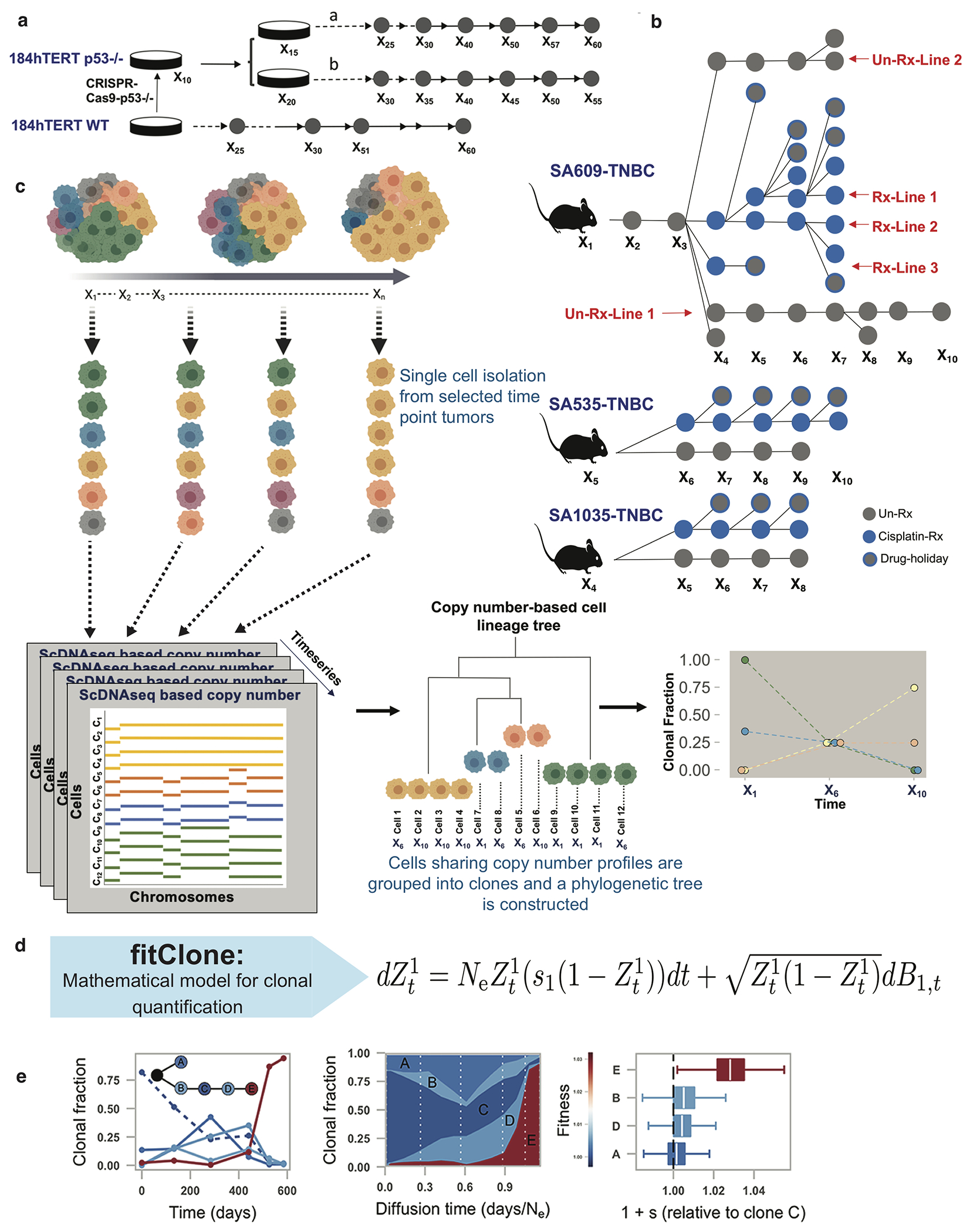
Schematic overview of experimental design for quantitatively modeling clone-specific fitness. Timeseries sampling from in vitro a) and PDX b) systems. Grey circles represent un-treated, blue represents Cisplatin treated and grey with a blue outline denotes drug-holiday samples. c) Clonal dynamics of cell populations observed over time. Whole genome single cell sequencing of timeseries samples gives copy number (left) that in turn is used to infer a phylogenetic tree (middle), and clonal fractions over time (right). d) fitClone: mathematical modeling of fitness with diffusion approximation to the K-type Wright-Fisher model. e) fitClone inputs of clonal dynamics measured over time series (left), and inferred trajectories (middle) and posterior distributions of fitness coefficients (right). Boxplots are as defined in Fig. 1b.

Extended Data Fig. 2.

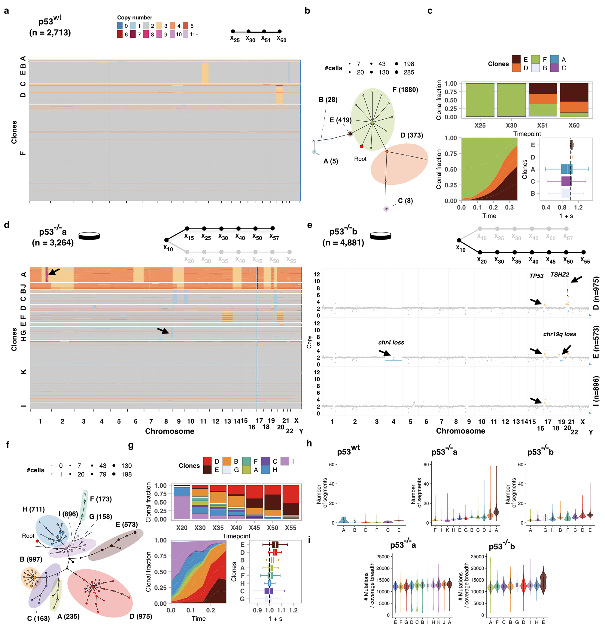
Impact of p53 mutation on fitness in 184hTERT cells. a) Heatmap representation of copy number profiles of 2,713 p53^wt cells, grouped in 6 phylogenetic clades. b) Phylogeny of cells over the timeseries p53^wt where nodes are groups of cells (scaled in size by number) with shared copy number genotype and edges represent distinct genomic breakpoints. Shaded areas represent clones. Tree root is denoted by the red circle. c) Observed clonal fractions over time, inferred trajectories and quantiles of the posterior distributions over selection coefficients of fitClone model fits to p53^wt with respect to the reference Clone F. d) Analogous to a but for p53^−/−a (n=3,264 cells p53^−/−a cells). e) Clonal genotypes of three representative clones for p53^−/−b showing high level amplification of TSHZ2 in Clone D, Chr4 loss in Clone E. Reference diploid Clone I is shown for comparison. f, g) Analogous to b, c but for p53^−/−b (n=4,881 p53^−/−b cells; reference Clone I). h) Number of segments per clone in hTERT WT and p53^−/−a and p53^−/−b branches. i) Number of mutations in p53^−/−a and p53^−/−b branches. Boxplots are as defined in Fig. 1b.

Extended Data Fig. 3.

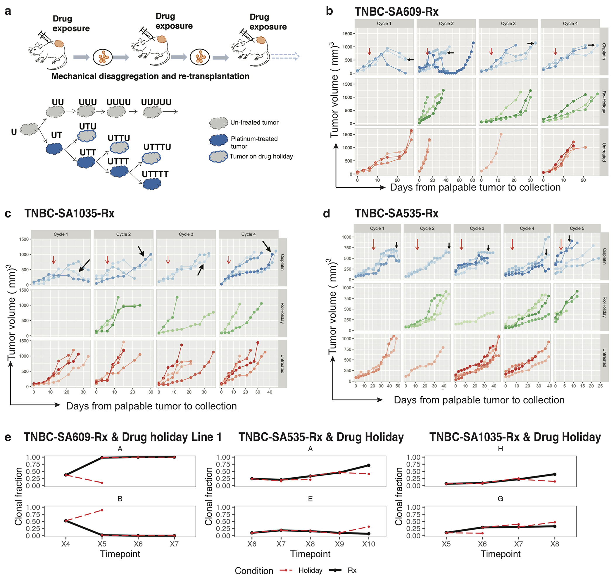
PDXs tumour growth and clonal dynamics with cisplatin. a) Experimental design of cisplatin treatment in PDX. The solid blue colour representing cisplatin treated tumours (UT,UTT,UTTT,UTTTT); blue outlined in grey as drug holiday (UTU,UTTU,UTTTU); grey as untreated series. b-d) Tumour response curves in TNBC-SA609, TNBC-SA535 and TNBC-SA1035 treated with Cisplatin (blue), in drug Holiday (green) and untreated (red) where each tumour replicate is shown in a different shade. The vertical axis on the right denotes the status of tumours and on the left denotes the tumour volumes. The top horizontal axis represents number of cisplatin cycles and at the bottom days from palpable tumours to collection. The red arrows indicate the start of treatment and the black arrows indicate the tumour sampled for scDNAseq. The bottom horizontal axis shows the tumour passage number. Each line in the big box is an individual tumour showing the growth over time. e) (top) Clonal trajectories of the clone with the highest inferred selection coefficient in the treatment regime (solid black line) and the drug holiday counterpart (dashed red line) at each timepoint, in the three TNBC PDX timeseries; (bottom) As the top row, but for a clone that grows back in the holiday regime.

Extended Data Fig. 4.

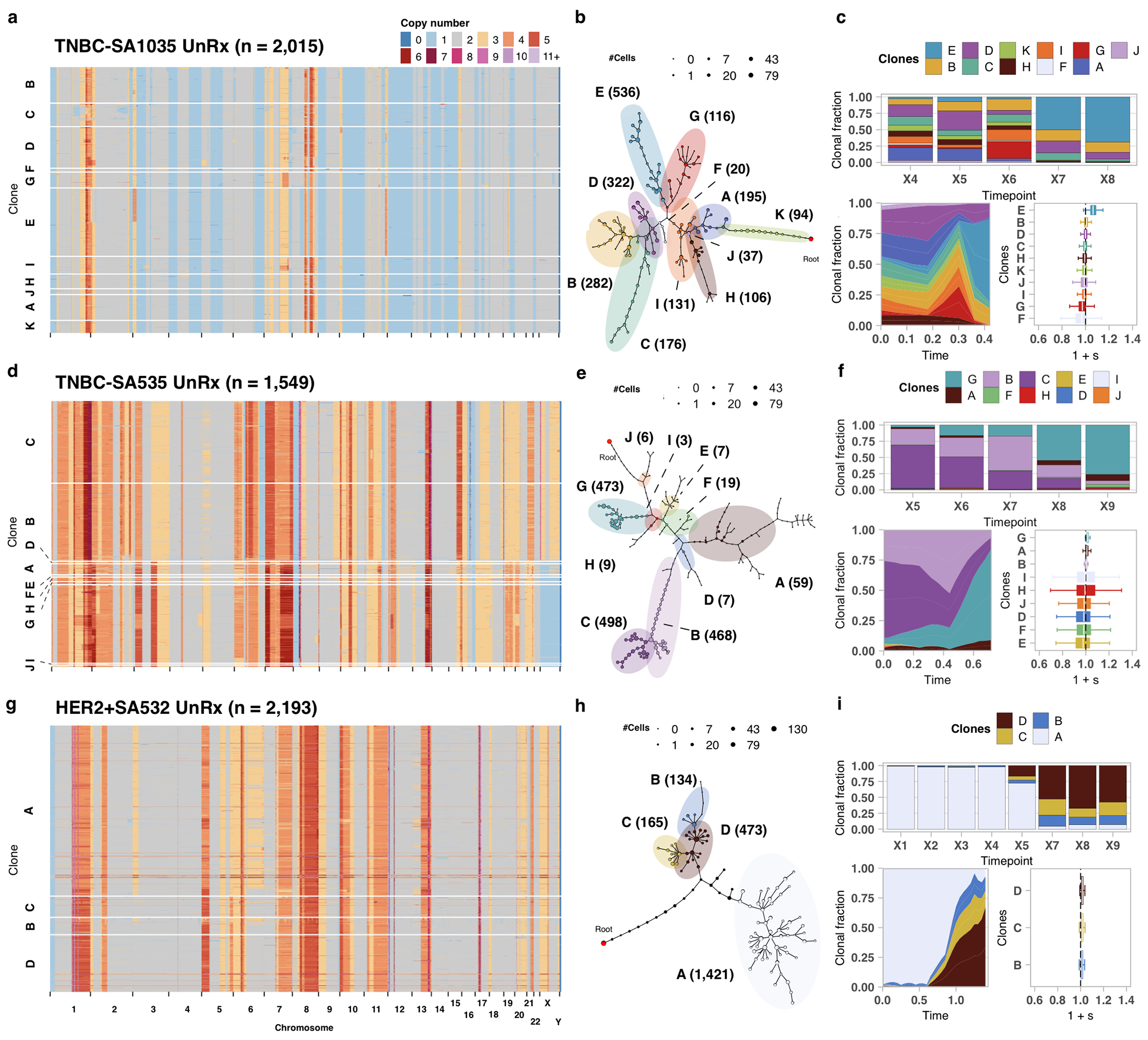
Comparison of fitness landscapes of breast cancer PDX models. a) Heatmap representation of copy number profiles of 2,015 cells from TNBC-SA1035, grouped in 11 phylogenetic clades. b) Phylogeny for TNBC-SA1035. c) Observed clonal fractions, inferred fitClone trajectories and quantiles of the selection coefficients with respect to the reference Clone A for the TNBC-SA1035 UnRx model. d-f) Analogous to a-c but for TNBC+SA535 (n=1,549 cells; reference Clone C). g-i) Analogous to a-c but for HER2+SA532 (n=2,193 cells; reference Clone A). Boxplots are as defined in Fig. 1b.

Extended Data Fig. 5.

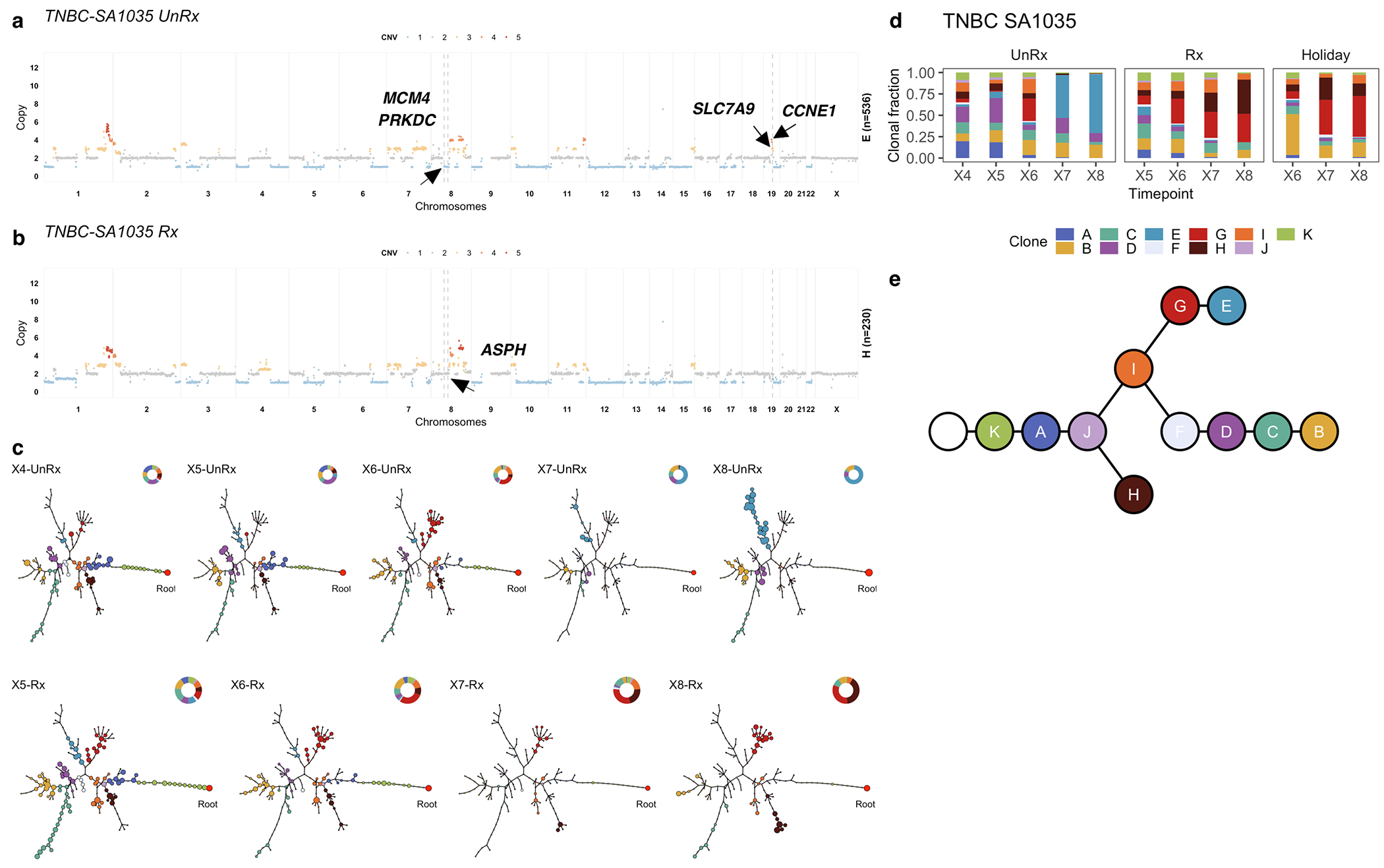
Impact of pharmacologic perturbation with cisplatin on fitness landscapes in TNBC-SA1035. a) Copy number genotype of Clone E from the untreated timeseries. b) Copy number genotype of clone H from treated timeseries (arrows indicate differences to Clone E). c) Evolution in absence of treatment and as a function of drug treatment. For each sample, the phylogeny with clonal abundance from DLP+ is shown, reflecting selection. d) The observed clonal abundances and e) the summarised clonal phylogenetic tree.

Extended Data Fig. 6.

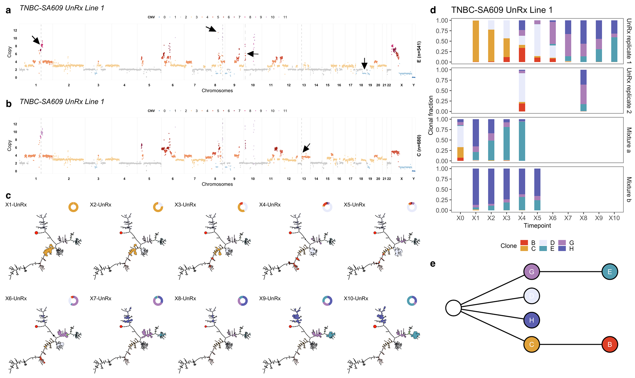
Tumour evolution in absence of pharmacologic perturbation in TNBC-SA609 line 1. a) Copy number genotype of Clone E and b) copy number genotype of Clone C, the reference clone (arrows indicate differences to Clone E). c) Evolution in absence of treatment. For each sample, the phylogeny with clonal abundance from DLP+ is shown, reflecting selection. d) The observed clonal abundances and e) the summarised clonal phylogenetic tree.

Extended Data Fig. 7.

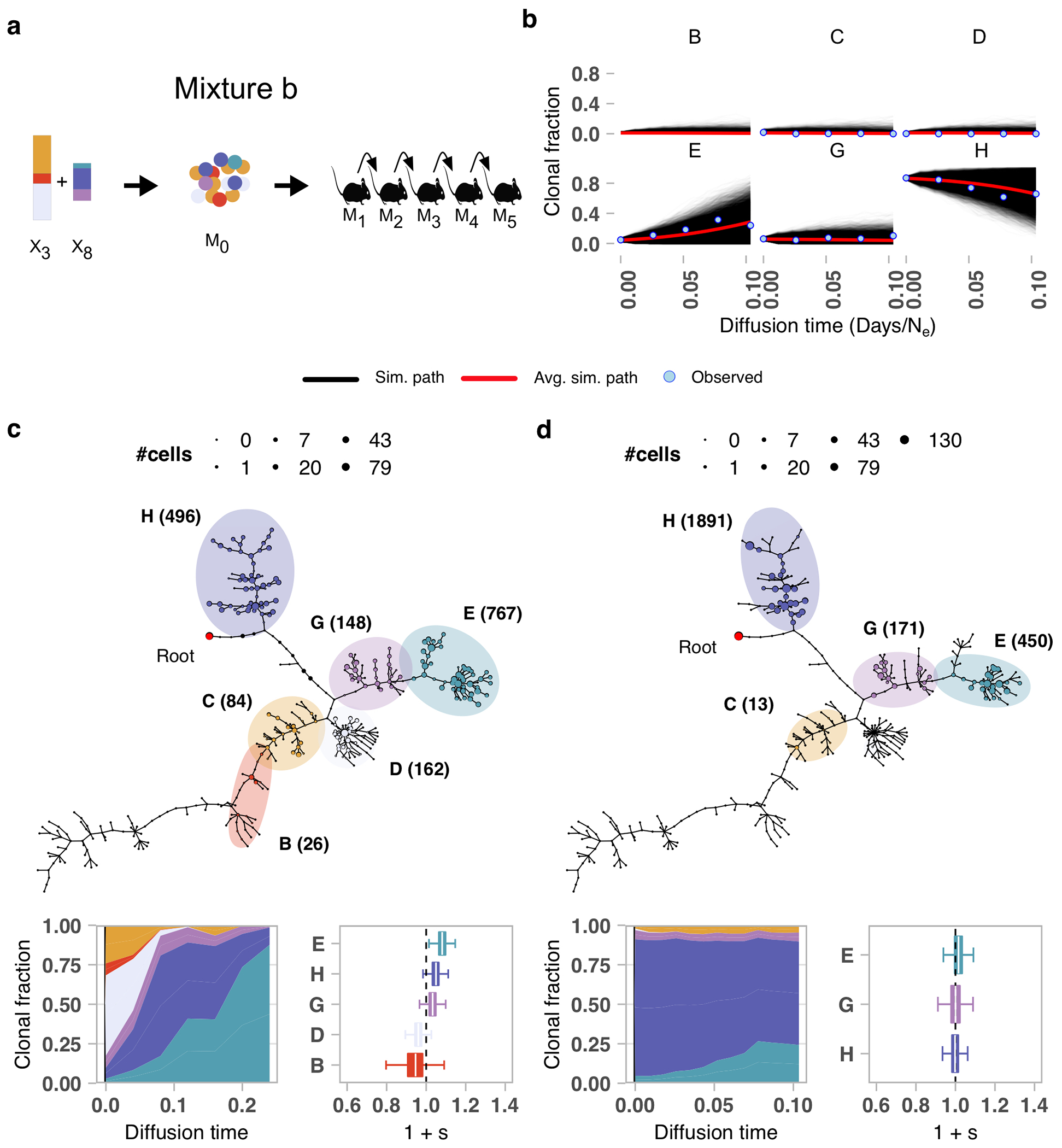
Mixture experiment in TNBC-SA609 PDX Line 1. a) Clonal proportions of TNBC-SA609 Line 1 X3 and X8 used to generate the initial mixture M0 and subsequent serial passaging, yielding 5 samples for mixture experiment b. b) Forward simulations from the original timeseries and starting population proportions in the initial experimental mixture b. Simulated trajectories are shown superimposed with mean simulation (red line) and observed clonal fractions (blue dots). The observation time is adjusted to match the simulation diffusion time. c) Summary phylogenetic tree, inferred trajectories and fitness coefficients (relative to reference Clone C) for mixture a. d) As in c but for mixture b (relative to reference Clone C). Boxplots are as defined in Fig. 1b.

Extended Data Fig. 8.

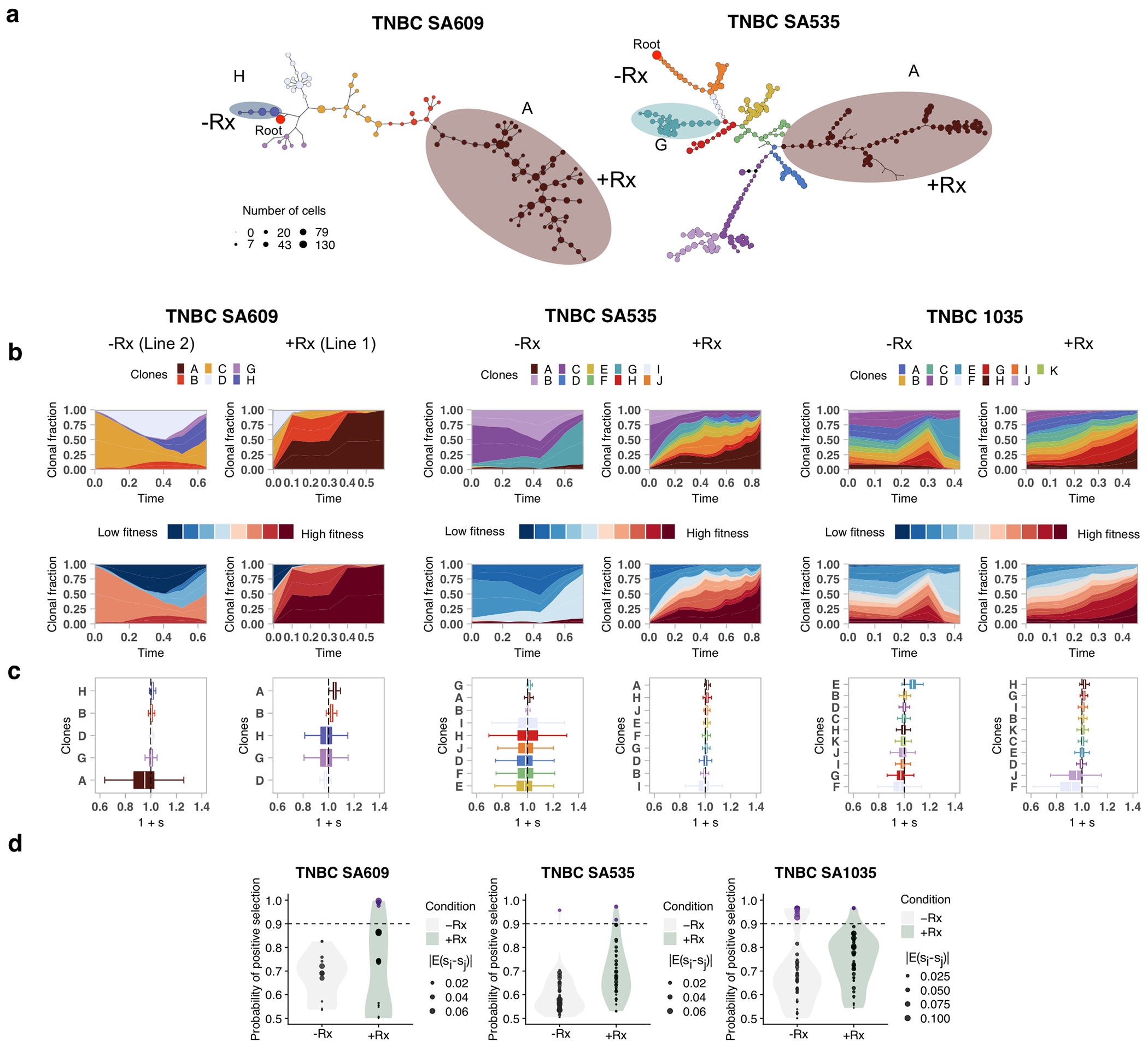
Fitness landscape reversal in early Cisplatin treatment in TNBC PDX models. In each column, the left and right sub-panels are from the untreated and treated branches respectively. a) Phylogenetic trees annotated with fittest clones in -Rx and Rx. b) Inferred trajectories, first coloured by clonal assignment, and then coloured by fitness rank, and c) quantiles of selection coefficients of fitClone model fits to each branch with respect to the reference Clone C in TNBC-SA609, Clone C in TNBC-SA535, and Clone A in TNBC-SA1035. e) Distribution over the probability of positive selection over pairs of clones for each series. Boxplots are as defined in Fig. 1b.

Extended Data Fig. 9.

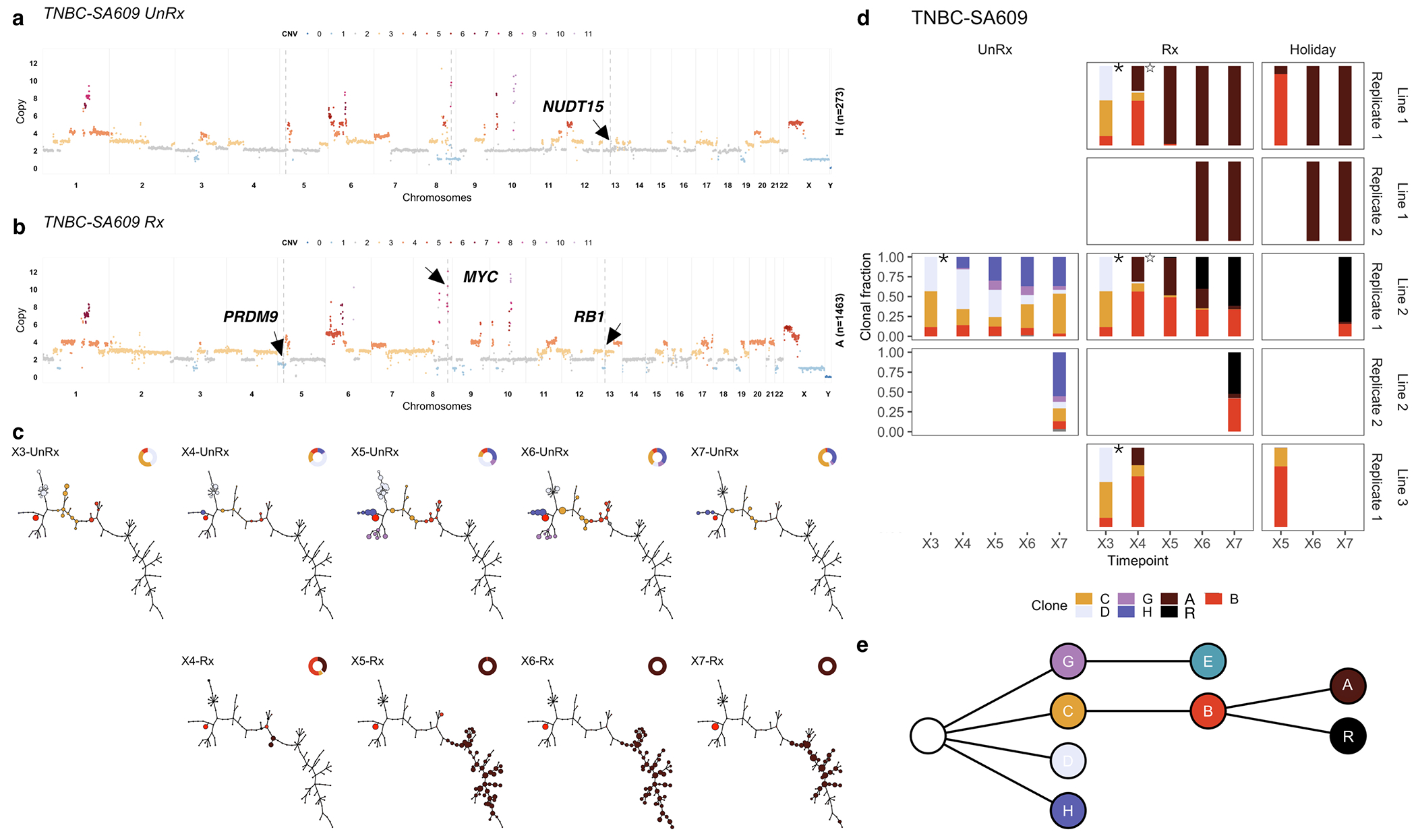
Impact of pharmacologic perturbation with cisplatin on fitness landscapes in TNBC-SA609. a) Copy number genotype of Clone H from untreated timeseries. b) Copy number genotype of Clone A from the treated timeseries (arrows indicate differences to Clone H). c) Evolution in absence of treatment (top) and as a function of treatment (bottom). For each sample, the phylogeny with clonal abundance from DLP+ is shown, reflecting selection. d) The observed clonal abundances. Starred timepoints are identical and reproduced to denote the identical starting point. e) Summarised clonal phylogenetic tree.

Extended Data Fig. 10.

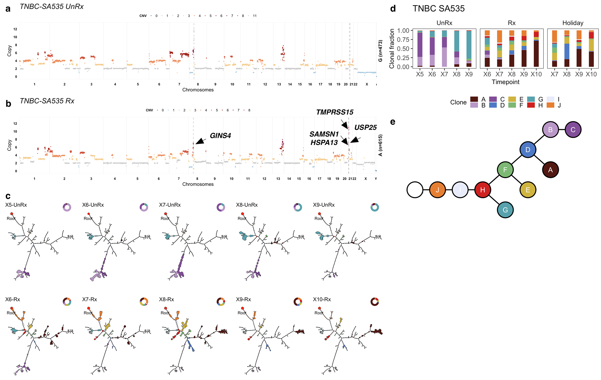
Impact of pharmacologic perturbation with cisplatin on fitness landscapes in TNBC-SA535. a) Copy number genotype of clone G from untreated timeseries. b) Copy number genotype of clone A from treated timeseries (arrows indicate differences to clone E). c) Evolution in absence of treatment and as a function of drug treatment. For each sample, the phylogeny with clonal abundance from DLP+ is shown, reflecting selection. d) The observed clonal abundances and e) the summarised clonal phylogenetic tree.

IMAXT Consortium members

Gregory J Hannon⁹, Giorgia Battistoni⁹, Dario Bressan⁹, Ian Gordon Cannell⁹, Hannah Casbolt⁹, Atefeh Fatemi⁹, Cristina Jauset⁹, Tatjana Kovačević⁹, Claire M Mulvey⁹, Fiona Nugent⁹, Marta Paez Ribes⁹, Isabella Pearsall⁹, Fatime Qosaj⁹, Kirsty Sawicka⁹, Sophia A Wild⁹, Elena Williams⁹, Samuel Aparicio^1,2, Emma Laks^1,2, Yangguang Li¹, Ciara H O’Flanagan¹, Austin Smith¹, Teresa Ruiz¹, Daniel Lai^1,2, Roth Andrew^2,4, Shankar Balasubramanian^9,10,11, Maximillian Lee^9,10, Bernd Bodenmiller¹², Marcel Burger¹², Laura Kuett¹², Sandra Tietscher¹², Jonas Windhager¹², Edward S Boyden¹³, Shahar Alon¹³, Yi Cui¹³, Amauche Emenari¹³, Dan Goodwin¹³, Emmanouil D Karagiannis¹³, Anubhav Sinha¹³, Asmamaw T Wassie¹³, Carlos Caldas¹⁴, Alejandra Bruna¹⁴, Maurizio Callari⁹, Wendy Greenwood⁹, Giulia Lerda⁹, Yaniv Eyal-Lubling¹⁴, Oscar M Rueda¹⁴, Abigail Shea¹⁴, Owen Harris¹⁵, Robby Becker¹⁵, Flaminia Grimaldi¹⁵, Suvi Harris¹⁵, Sara Lisa Vogl¹⁵, Joanna Weselak¹⁵, Johanna A Joyce¹⁶, Spencer S Watson¹⁶, Sohrab P Shah³, Andrew McPherson³, Ignacio Vázquez-García³, Simon Tavare’^9,17,18, Khanh N Dinh¹⁷, Eyal Fisher⁹, Russell Kunes ¹⁷, Nicholas A Walton¹⁹, Mohammad Al Sa’d¹⁹, Nick Chornay¹⁹, Ali Dariush¹⁹, Eduardo A González-Solares¹⁹, Carlos González-Fernández¹⁹, Aybüke Küpcü Yoldaş ¹⁹, Neil Millar¹⁹, Tristan Whitmarsh¹⁹, Xiaowei Zhuang^20,21,22, Jean Fan^20,21,22, Hsuan Lee^20,21,22, Leonardo A Sepúlveda^20,21,22, Chenglong Xia^20,21,22, Pu Zheng^20,21,22,

9. Cancer Research UK Cambridge Institute, Li Ka Shing Centre, University of Cambridge, Cambridge CB2 0RE, UK

10. Department of Chemistry, University of Cambridge, Lensfield Road, Cambridge, CB2 1EW, UK

11. School of Clinical Medicine, University of Cambridge, Cambridge, CB2 0SP, UK affx7

12. Department of Quantitative Biomedicine, , University of Zurich, Zurich 8057, Switzerland

13. McGovern Institute, Departments of Biological Engineering and Brainand Cognitive Sciences, Massachusetts Institute of Technology,Cambridge, Massachusetts, USA

14. Department of Oncology and Cancer Research UK Cambridge Institute, University of Cambridge, Cambridge, CB2 0RE, UK

15. Súil Interactive Ltd, Dame Lane, Dublin, UK

16. Department of Oncology and Ludwig Institute for Cancer Research, University of Lausanne, Lausanne, Switzerland

17. Herbert and Florence Irving Institute for Cancer Dynamics, Columbia University, New York, NY, USA

18. New York Genome Center, New York, NY, USA

19. Institute of Astronomy, University of Cambridge, Madingley Road, Cambridge, CB3 0HA, UK

20. Howard Hughes Medical Institute, Harvard University, Cambridge, MA 02138, USA

21. Department of Physics, Harvard University, Cambridge, MA 02138, USA

22. Department of Chemistry and Chemical Biology, Harvard University, Cambridge, MA 02138, USA

Data Availability

Raw sequencing data for DLP+ and 10x scRNASeq is available from the European Genome-Phenome archive at: [https://ega-archive.org/studies/EGAS00001004448]. Single cell data from this report may be visualized in an instance of our scWGS exploration platform, Alhena, available at: [https://www.cellmine.org].

References

- 1.Gerstung M et al. The evolutionary history of 2,658 cancers. en. Nature 578, 122–128 (2020). [DOI] [PMC free article] [PubMed] [Google Scholar]
- 2.Williams MJ et al. Quantification of subclonal selection in cancer from bulk sequencing data. en. Nat. Genet 50, 895–903 (2018). [DOI] [PMC free article] [PubMed] [Google Scholar]
- 3.Salichos L, Meyerson W, Warrell J & Gerstein M Estimating growth patterns and driver effects in tumor evolution from individual samples. Nature communications 11, 1–14 (2020). [DOI] [PMC free article] [PubMed] [Google Scholar]
- 4.Shah SP et al. The clonal and mutational evolution spectrum of primary triple-negative breast cancers. Nature 486, 395–399 (2012). [DOI] [PMC free article] [PubMed] [Google Scholar]
- 5.Li Y et al. Patterns of somatic structural variation in human cancer genomes. en. Nature 578, 112–121 (2020). [DOI] [PMC free article] [PubMed] [Google Scholar]
- 6.Nik-Zainal S et al. Landscape of somatic mutations in 560 breast cancer whole-genome sequences. Nature 534, 47 (2016). [DOI] [PMC free article] [PubMed] [Google Scholar]
- 7.Curtis C et al. The genomic and transcriptomic architecture of 2,000 breast tumours reveals novel subgroups. Nature 486, 346–352 (2012). [DOI] [PMC free article] [PubMed] [Google Scholar]
- 8.Wright S The distribution of gene frequencies in populations. Proceedings of the National Academy of Sciences of the United States of America 23, 307 (1937). [DOI] [PMC free article] [PubMed] [Google Scholar]
- 9.Tataru P, Simonsen M, Bataillon T & Hobolth A Statistical inference in the Wright–Fisher model using allele frequency data. Systematic biology 66, e30–e46 (2017). [DOI] [PMC free article] [PubMed] [Google Scholar]
- 10.Vasan N, Baselga J & Hyman DM A view on drug resistance in cancer. en. Nature 575, 299–309 (2019). [DOI] [PMC free article] [PubMed] [Google Scholar]
- 11.Ben-David U & Amon A Context is everything: aneuploidy in cancer. Nature Reviews Genetics 21, 44–62 (2020). [DOI] [PubMed] [Google Scholar]
- 12.Sunshine AB et al. The fitness consequences of aneuploidy are driven by condition-dependent gene effects. PLoS Biol 13, e1002155 (2015). [DOI] [PMC free article] [PubMed] [Google Scholar]
- 13.Sheltzer JM, Torres EM, Dunham MJ & Amon A Transcriptional consequences of aneuploidy. Proceedings of the National Academy of Sciences 109, 12644–12649 (2012). [DOI] [PMC free article] [PubMed] [Google Scholar]
- 14.Williams MJ, Werner B, Barnes CP, Graham TA & Sottoriva A Identification of neutral tumor evolution across cancer types. en. Nat. Genet 48, 238–244 (2016). [DOI] [PMC free article] [PubMed] [Google Scholar]
- 15.Nik-Zainal S et al. The life history of 21 breast cancers. Cell 149, 994–1007 (2012). [DOI] [PMC free article] [PubMed] [Google Scholar]
- 16.Martincorena I et al. Universal patterns of selection in cancer and somatic tissues. Cell 171, 1029–1041 (2017). [DOI] [PMC free article] [PubMed] [Google Scholar]
- 17.Khan KH et al. Longitudinal liquid biopsy and mathematical modeling of clonal evolution forecast time to treatment failure in the PROSPECT-C phase II colorectal cancer clinical trial. Cancer discovery 8, 1270–1285 (2018). [DOI] [PMC free article] [PubMed] [Google Scholar]
- 18.Gerlinger M et al. Genomic architecture and evolution of clear cell renal cell carcinomas defined by multiregion sequencing. Nat. Genet 46, 225–233 (2014). [DOI] [PMC free article] [PubMed] [Google Scholar]
- 19.Jamal-Hanjani M et al. Tracking the evolution of non–small-cell lung cancer. New England Journal of Medicine 376, 2109–2121 (2017). [DOI] [PubMed] [Google Scholar]
- 20.López S et al. Interplay between whole-genome doubling and the accumulation of deleterious alterations in cancer evolution. Nature genetics 52, 283–293 (2020). [DOI] [PMC free article] [PubMed] [Google Scholar]
- 21.McPherson A et al. Divergent modes of clonal spread and intraperitoneal mixing in high-grade serous ovarian cancer. Nat. Genet 48,758–767 (2016). [DOI] [PubMed] [Google Scholar]
- 22.Good BH, McDonald MJ, Barrick JE, Lenski RE & Desai MM The dynamics of molecular evolution over 60,000 generations. en. Nature 551, 45–50 (2017). [DOI] [PMC free article] [PubMed] [Google Scholar]
- 23.Dorri F et al. Efficient Bayesian inference of phylogenetic trees from large scale, low-depth genome-wide single-cell data. bioRxiv. doi: 10.1101/2020.05.06.058180.eprint: https://www.biorxiv.org/content/early/2020/05/07/2020.05.06.058180.full.pdf.https://www.biorxiv.org/content/early/2020/05/07/2020.05.06.058180 (2020). [DOI] [Google Scholar]
- 24.Burleigh A et al. A co-culture genome-wide RNAi screen with mammary epithelial cells reveals transmembrane signals required for growth and differentiation. en. Breast Cancer Res. 17, 4(2015). [DOI] [PMC free article] [PubMed] [Google Scholar]
- 25.Vega M. R. d. l., de la Vega MR, Chapman E & Zhang DD NRF2 and the Hallmarks of Cancer 2018. [DOI] [PMC free article] [PubMed] [Google Scholar]
- 26.Cancer Genome Atlas Network. Comprehensive molecular portraits of human breast tumours. en. Nature 490, 61–70 (2012). [DOI] [PMC free article] [PubMed] [Google Scholar]
- 27.Patch A-M et al. Whole-genome characterization of chemoresistant ovarian cancer. Nature 521, 489–494 (2015). [DOI] [PubMed] [Google Scholar]
- 28.Laks E et al. Clonal Decomposition and DNA Replication States Defined by Scaled Single-Cell Genome Sequencing. en. Cell 179, 1207–1221.e22 (2019). [DOI] [PMC free article] [PubMed] [Google Scholar]
- 29.Hather G et al. Growth Rate Analysis and Efficient Experimental Design for Tumor Xenograft Studies: Supplementary Issue: Array Platform Modeling and Analysis (A). Cancer Informatics 13, CIN-S13974 (2014). [DOI] [PMC free article] [PubMed] [Google Scholar]
- 30.Bielski CM et al. Genome doubling shapes the evolution and prognosis of advanced cancers. en. Nat. Genet 50, 1189–1195 (2018). [DOI] [PMC free article] [PubMed] [Google Scholar]
- 31.Bakhoum SF et al. Chromosomal instability drives metastasis through a cytosolic DNA response. en. Nature 553, 467–472 (2018). [DOI] [PMC free article] [PubMed] [Google Scholar]
- 32.Davoli T, Uno H, Wooten EC & Elledge SJ Tumor aneuploidy correlates with markers of immune evasion and with reduced response to immunotherapy. en. Science 355 (2017). [DOI] [PMC free article] [PubMed] [Google Scholar]
- 33.Acar A et al. Exploiting evolutionary steering to induce collateral drug sensitivity in cancer. Nature communications 11, 1–14 (2020). [DOI] [PMC free article] [PubMed] [Google Scholar]
- 34.Eirew P et al. Dynamics of genomic clones in breast cancer patient xenografts at single-cell resolution. Nature 518, 422–426 (2015). [DOI] [PMC free article] [PubMed] [Google Scholar]
- 35.Li D et al. Enhanced tumor suppression by adenoviral PTEN gene therapy combined with cisplatin chemotherapy in small-cell lung cancer. Cancer gene therapy 20, 251–259 (2013). [DOI] [PubMed] [Google Scholar]
- 36.Wang Y et al. Klotho sensitizes human lung cancer cell line to cisplatin via PI3k/Akt pathway. PloS one 8 (2013). [DOI] [PMC free article] [PubMed] [Google Scholar]
- 37.OâFlanagan CH et al. Dissociation of solid tumor tissues with cold active protease for single-cell RNA-seq minimizes conserved collagenase-associated stress responses. Genome biology 20, 1–13 (2019). [DOI] [PMC free article] [PubMed] [Google Scholar]
- 38.Roth A et al. PyClone: statistical inference of clonal population structure in cancer. Nature methods 11, 396–398 (2014). [DOI] [PMC free article] [PubMed] [Google Scholar]
- 39.Beaumont MA, Cornuet J-M, Marin J-M & Robert CP Adaptive approximate Bayesian computation. Biometrika 96, 983–990 (2009). [Google Scholar]
- 40.Foll M et al. Influenza virus drug resistance: a time-sampled population genetics perspective. PLoS Genet 10, e1004185 (2014). [DOI] [PMC free article] [PubMed] [Google Scholar]
- 41.Bollback JP, York TL & Nielsen R Estimation of 2Nes from temporal allele frequency data. Genetics 179, 497–502 (2008). [DOI] [PMC free article] [PubMed] [Google Scholar]
- 42.Malaspinas A-S, Malaspinas O, Evans SN & Slatkin M Estimating allele age and selection coefficient from time-serial data. Genetics 192, 599–607 (2012). [DOI] [PMC free article] [PubMed] [Google Scholar]
- 43.Ferrer-Admetlla A, Leuenberger C, Jensen JD & Wegmann D An approximate markov model for the Wright–Fisher diffusion and its application to time series data. Genetics 203, 831–846 (2016). [DOI] [PMC free article] [PubMed] [Google Scholar]
- 44.Beskos A, Roberts GO, et al. Exact simulation of diffusions. The Annals of Applied Probability 15, 2422–2444 (2005). [Google Scholar]
- 45.Pollock M, Johansen AM, Roberts GO, et al. On the exact and ε-strong simulation of (jump) diffusions. Bernoulli 22, 794–856 (2016). [Google Scholar]
- 46.Jenkins PA, Spano D, et al. Exact simulation of the Wright–Fisher diffusion. The Annals of Applied Probability 27, 1478–1509 (2017). [Google Scholar]
- 47.Blanchet J Exact simulation for multivariate Itô diffusions (2017). [Google Scholar]
- 48.Jorde P, Palm S & Ryman N Estimating genetic drift and effective population size from temporal shifts in dominant gene marker frequencies. Molecular Ecology 8, 1171–1178 (1999). [DOI] [PubMed] [Google Scholar]
Associated Data
This section collects any data citations, data availability statements, or supplementary materials included in this article.
Supplementary Materials
Data Availability Statement