The numerical solution of high dimensional variable-order time fractional diffusion equation via the singular boundary method

Graphical abstract

Highlights

• •The 3D variable-order time fractional variable-order time fractional diffusion is generated.
• •An efficient meshless method is proposed for numerical solution of the new problem.
• •The proposed approach is established upon the singular boundary method.
• •The method accuracy is examined by some numerical examples on various geometries.
• •The method can be extended for other types of variable-order fractional problems.

Abstract

Introduction

This study describes a novel meshless technique for solving one of common problem within cell biology, computer graphics, image processing and fluid flow. The diffusion mechanism has extremely depended on the properties of the structure.

Objectives

The present paper studies why diffusion processes not following integer-order differential equations, and present novel meshless method for solving. diffusion problem on surface numerically.

Methods

The variable- order time fractional diffusion equation (VO-TFDE) is developed along with sense of the Caputo derivative for $(0<\alpha (t)<1)$. An efficient and accurate meshfree method based on the singular boundary method (SBM) and dual reciprocity method (DRM) in concomitant with finite difference scheme is proposed on three-dimensional arbitrary geometry. To discrete of the temporal term, the finite diffract method (FDM) is utilized. In the spatial variation domain; the proposal method is constructed two part. To evaluating first part, fundamental solution of (VO-TFDE) is transformed into inhomogeneous Helmholtz-type to implement the SBM approximation and other part the DRM is utilized to compute the particular solution.

Results

The stability and convergent of the proposed method is numerically investigated on high dimensional domain. To verified the reliability and the accuracy of the present approach on complex geometry several examples are investigated.

Conclusions

The result of study provides a rapid and practical scheme to capture the behavior of diffusion process.

Introduction

The diffusion model is known as one of the ubiquitous phenomena in nature. The diffusion itself has been also recognized as a basic moving process involved in the evolution of numerous non-balance systems towards balance. Accordingly, the classical diffusion equation reveals how a molecule is released from one zone with a higher concentration zone into a lower concentration zone, to the condition in which it can become evenly dispersed. As well, the anomalous transport of the particles in the diffusion process can be modeled by wake effects randomly. Considering the motion of the particles in complex media, commonly having disordered microscopic sub-structures, the classical diffusion equation may not coincide with the data obtained from the empirical research and it no longer valid Gaussian behavior. In this sense, the fractional differential equations (FDEs) can describe and simulate behaviors of various dynamic processing phenomena beyond the traditional operators in a very robust and reliable way. Such differential operators emerge in modeling a extremely widespread throughout the science and technology involving e.g., healthcare [46], [48], [3], [6], [36], [54], [44], [14], [41], [46], contaminant transport [7], [57], polymer networks [2], wave propagation [35], control [29], [50], [39], [31], physics [28], [58], [47], [4], [5], [21], [22], [20], [19] and engineering [30], [57], [36]. Recently, the FDEs have further established strategies to capture different models of dynamic processing in complex media and include diffusion phenomena due to their ability to interpret many non-Gaussian statistics [19], [43], [49].

The diffusion mechanism has extremely depended on the properties of the structure. More explicitly speaking, diffusion is an interactive phenomena in nature in a sense that it keeps on changing gradually according to interactants’ instantaneous in time and/or spacein eventually, it has been become evenly dispersed within the corresponding structure. Hence, diffusion processes not following integer-order differential equations, cannot adequately capture the dynamic physical phenomena and processes in complex medium. Adapting order of the diffusion equation are critical at any time or space level. More precisely, we consider a field-variable, variable-order fractional (VOF), which can be introduced as an extension of the classical fractional calculus. In fact, (VOF) is more realistic and accurate to the interpretation of many dynamical systems and processes, particularly those phenomena associated with inhomogeneous medium. The last two decades, researcher have been numerous endeavoring to decipher the behavior anomalous solute diffusion and migration in heterogeneous physical systems. There have been several other applications with variable-order models. It should be emphasized that due to kernel of the (VOF) has a variable-exponent, solving analytically is extremely difficult and tedious procedure.

Recent experiments have demonstrated that some phenomena have transient behaviors varying with time evolution or spatial variation or even spatiotemporal changes. Using the constant-order FDEs may not be an effective and efficient method to understand transient behaviors. To rectify such a problem, the variable-order (VO) FDEs (VO-FDEs) have been proposed to capture. In such transient diffusive states, the VO index is time-dependent, space- dependent, spatial dependent, or spatiotemporal- dependent [55], [56], [34]. A challenging problem arising in the VO-FDEs is difficult to obtain analytical solutions, even sometimes beyond the limits of current knowledge. Thus, approximate solutions are sought. Proposing accurate and reliable numerical/approximate approaches can accordingly play a crucial role in simulation of the VO-FDEs. There are widely different effective numerical methods to assess the VO-FDEs. Such techniques include mesh-based methods e.g., including finite difference method (FDM), finite element method (FEM), and boundary element method (BEM) [32], [13], [33], as well as some kernel-based methods such as Fourier transform (FT) [8] and wavelets transform (WT) [24], introduced for solving the constant FDEs and the VO ones. Each of these schemes might have their own strengths and challenges, depending on the application addressed. It is of note that although these methods are very effective in solving the VO-FDEs, they typically require sophisticated algorithms. There are also several drawbacks associated with these approaches including central processing unit (CPU) time, required re-meshing, burdensome meshing, etc. Furthermore, these numerical/approximate approaches may lead to reduced accuracy in high-dimensional problems, irregular geometries or meshes, and even non-smooth domains.

Much more recently, meshless methods with radial basis functions (RBFs) have been expanded as valuable alternatives to overcome the limits of traditional mesh bases on many phenomena in the realm of science and engineering [60], [59], [62], [63], [64]. Unlike the traditional basis functions and mesh-based methods, the RBFs can be simply appended and reduced without a burdensome meshing of node point [26], [27], [25]. The most significant superiority of meshless methods is associated with being straightforward to implement, truly meshless, independent of dimensionality and high-order continuous shape functions over other numerical methods [51], [52], [53].

The method of fundamental solution (MFS) is introduced as RBF collocation techniques the boundary- type. To eschew singularity of fundamental solution, distributing source points on auxiliary boundary is choose outside computational boundary (physical boundary) [37]. The MFS have drawn scientific attention due to highly accurate, truly meshless and straightforward in recent years [16]. Although the MFS has been mentioned in many research as efficient method that has high accuracy in solving differential equation despite a challenging approach arising in this domain is that the determining interval auxiliary boundary and computational domain is often arbitrary. Finding the optimal location of fictitious boundary is time consuming process and still open to dispute. In [9], [11], Chen et al. to overcome this shortcoming, proposed the SBM base on origin intensity factors concept. In this approach introduced sense of (OIFs) due to proper performance in interpolation of scattering data and developed the MFS method as meshless method for problem with irregular geometry. The conception of OLF makes possible the selection boundary computational domain as location of source points. It is worth mentioning that entire feature of the MFS is adapted with SBM.

To extant this approach, subtracting and adding-back techniques along with inverse interpolation approaches, are being employed to assess the OIFs to isolate the source singularity of the fundamental solution and its derivative regarding the Dirichlet and the Neumann boundary conditions respectively. In recent years, the SBM formulations are becoming popular in a wide different science and engineering applications such as transient diffusion problems [10], acoustic [17].

As we are mentioned above, the SMB turns out to be an effective alternative to mesh-based computational methods for high-dimensional structures. The mesh-based method should mostly expand estimates of the metric tensor and other geometric quantities associated with the structure shape. On the other hand, two-dimensional (2D) models may be often utilized instead of 3D ones because of high computational costs and low computational speed. However, exploiting 3D structures to explain the mechanical behavior of bodies and the application of external forces to various physical phenomena is vital. To the best of authors’ knowledge, there is insufficient investigation with excellent numerical approaches to cover high- dimensional structures. 3D models arising in diverse science and engineering fields include transport of surfactants within bubbles and thin films [23], colloidal aggregation within fluid interfaces [15], fractional viscoelasticity [1], [38] and sliding mode control (SMC) [1], [61].

The main purpose of this investigation is to developed the SBM to solve both constant TFDEs- and VO ones. To decline storage requirements in the methodology of this paper, the FDM was used to discretize the time domain and to evaluating fundamental solution of (VO-TFDE) is transformed into inhomogeneous Helmholtz-type to approximate through the SBM. It should be pointed out that the SBM, boundary type approach as similar like MFS and BEM can be deal with homogeneous problem. Hance, it is adapted with dual reciprocity method (DRM) for space semi-discretization of the derived inhomogeneous equations. In this sense, the DRM is utilized to achieve the particular solution and the SBM is applied to compute the homogeneous one. Eventfully, the solution of the problem can be archived by aggregate of the particular solutions and the homogeneous. Thus, with the compounded properties of the DRM and the SBM, the numerical approximation solution base on meshless scheme is archived the inhomogeneous and time-dependent problems. To the best of the authors’ knowledge, the present study is the first attempt focused on the SBM to evaluate 3D VO-TFDE. The rest of the paper is organized as follows. In Section 2, after brief introduction of sense of the Caputo derivative for VO fractional followed by proposal method is described and derived on VO-TFDE. In Section 3, several conceptual numerical examples to demonstrates the reliability and the efficiency of the proposal technics and numerical results are compared with their analytical solution. Eventually, in Section 4, is devoted to a conclusions.

Numerical procedure: The Singular boundary method

Problem definition

The main objective of the present study is to introduce the VO-TFDEs on any arbitrary 3D domains and to propose a mesh-free method based on the SBM for its numerical solution. Thus, the following problem is investigated:

$$\frac{{\partial }^{\alpha \left(t\right)}u(\mathbf{x},t)}{\partial t^{\alpha \left(t\right)}}=A\mathrm{\Delta }u(\mathbf{x},t)-\mu u(\mathbf{x},t)+g(\mathbf{x},t),0<\alpha \left(t\right)<1,\mathbf{x}\in \mathrm{\Omega },t\in (0,T),$$ (1)

subject to the initial conditions:

$$u(\mathbf{x},0)=u_0\left(\mathbf{x}\right),\mathbf{x}\in \mathrm{\Omega },$$ (2)

The Dirichlet and the Neumann boundary conditions in their appropriate forms are:

$$u(\mathbf{x},t)=h_1(\mathbf{x},t),\mathbf{x}\in {\mathrm{\Gamma }}_D,t\in (0,T),$$ (3)

$$q(\mathbf{x},t)=\frac{\partial u(\mathbf{x},t)}{\partial n}=h_2(\mathbf{x},t),\mathbf{x}\in {\mathrm{\Gamma }}_N,t\in (0,T),$$ (4)

wherein, $\mathrm{\Delta }$ denotes the Laplacian operator, i.e., $\frac{{\partial }^2}{\partial x^2}+\frac{{\partial }^2}{\partial y^2}$ A is diffusion coefficient, and $\mu$ refers to reaction coefficient. As well, $g(\mathbf{x},t)$ represents a given function, $u_0\left(\mathbf{x}\right)$ stands for prescribed initial functions, $h_1(\mathbf{x},t)$ and $h_2(\mathbf{x},t)$ are prescribed boundary functions, ${\mathrm{\Gamma }}_N$ shows bound region $\mathrm{\Omega },n$ indicatives unit outward normal vector on boundary of domain ${\mathrm{\Gamma }}_N$. Moreover, ${\partial }^{\alpha \left(t\right)}/\partial t^{\alpha \left(t\right)}$ is expressed in term of VO fractional derivative of order where $\alpha \left(t\right)$ represent prescribed as the field variable basis in the interval $(0,1)$. Among of several possibilities for definitions the VO fractional derivative definitions, the Coimbra’s definition is chosen [12]:

$$\frac{{\partial }^{\alpha \left(t\right)}u(\mathbf{x},t)}{\partial t^{\alpha \left(t\right)}}=\frac{1}{\mathrm{\Gamma }(1-\alpha (t\left)\right)}{\int }_0^t\frac{\partial u(\mathbf{x},s)}{\partial s}\frac{\mathit{ds}}{{(t-s)}^{\alpha \left(t\right)}}+\frac{\left(u\right(\mathbf{x},t_{0+})-u(\mathbf{x},t_{0-}\left)\right)t^{-\alpha \left(t\right)}}{\mathrm{\Gamma }(1-\alpha (t\left)\right)}\text{.}$$

This definition only employs the integer order derivatives existing in the initial condition and it may be expanded easliy to physical deems. Furthermore, the Coimbra’s definition is addressed as the following Caputo-type definition for the continuous functions:

$$\frac{{\partial }^{\alpha \left(t\right)}u(\mathbf{x},t)}{\partial t^{\alpha \left(t\right)}}=\frac{1}{\mathrm{\Gamma }(1-\alpha (t\left)\right)}{\int }_0^t\frac{\partial u(\mathbf{x},s)}{\partial s}\frac{\mathit{ds}}{{(t-s)}^{\alpha \left(t\right)}}\text{.}$$ (5)

Hereupon, if $\alpha \left(t\right)$ is deal with a constant, this definition is transformed into the Caputo derivative definition [45].

The Finite difference approximation for time discretisation

Here, the VO time fractional derivative is discretized long with the FDM. Assume $t_k=k\delta t,k=0,1,\dots ,K$, where $\delta t=\frac{T}{K}$ and suppose $u(\mathbf{x},t)$ is continuous. The time fractional derivative with VO ${\partial }^{\alpha \left(t\right)}u(\mathbf{x},t)/\partial t^{\alpha \left(t\right)}$ at $t=t_{k+1}$ than is Eq. (5) can be expressed as follows:

$$\begin{array}{cc}\hfill \frac{{\partial }^{\alpha \left(t_{k+1}\right)}u(\mathbf{x},t_{k+1})}{\partial t^{\alpha \left(t\right)}}=& \frac{1}{\mathrm{\Gamma }(1-\alpha (t_{k+1}\left)\right)}{\int }_0^{(k+1)\delta t}\frac{\partial u(\mathbf{x},s)}{\partial s}\frac{\mathit{ds}}{{(t_{k+1}-s)}^{\alpha \left(t_{k+1}\right)}}\hfill \\ \hfill & =\frac{1}{\mathrm{\Gamma }(1-\alpha (t_{k+1}\left)\right)}{\displaystyle \sum _{j=0}^k}\frac{u(\mathbf{x},t_{j+1})-u(\mathbf{x},t_j)}{\delta t}{\int }_{j\delta t}^{(j+1)\delta t}\frac{1}{{(t_{k+1}-s)}^{\alpha \left(t_{k+1}\right)}}\mathit{ds}\hfill \end{array}$$ (6)

$$\begin{array}{cc}\hfill & =\frac{\delta t^{-\alpha \left(t_{k+1}\right)}}{\mathrm{\Gamma }(2-\alpha (t_{k+1}\left)\right)}{\displaystyle \sum _{j=0}^k}{\omega }_j(\mathbf{x},t_k)\left[u\right(\mathbf{x},t_{k+1-j})-u(\mathbf{x},t_{k-j}\left)\right]\hfill \\ \hfill & ={\zeta }^k\left[u(\mathbf{x},t_{k+1})-u(\mathbf{x},t_k)+{\displaystyle \sum _{j=1}^k}{\omega }_j(\mathbf{x},t_k)\left[u\right(\mathbf{x},t_{k-j+1})-u(\mathbf{x},t_{k-j}\left)\right]\right],\hfill \end{array}$$

where

$$\begin{array}{c}{\zeta }^k=\frac{\delta t^{-\alpha \left(t_{k+1}\right)}}{\mathrm{\Gamma }(2-\alpha (t_{k+1}\left)\right)}\hfill \\ {\omega }_j(\mathbf{x},t_k)={(j+1)}^{1-\alpha \left(t_{k+1}\right)}-j^{1-\alpha \left(t_{k+1}\right)},j=0,1,\cdots ,K-1\text{.}\hfill \end{array}$$ (7)

The following property has been shown previously in [18]

$$\left\{\begin{array}{c}{\omega }_j(\mathbf{x},t_k)>0,j=0,1,\dots ,k,\hfill \\ 1={\omega }_0(\mathbf{x},t_k)>{\omega }_1(\mathbf{x},t_k)>\dots >{\omega }_k(\mathbf{x},t_k),{\omega }_k(\mathbf{x},t_k)\to 0\mathit{as}k\to \infty \hfill \\ {\displaystyle \sum _{j=0}^k}\left({\omega }_j\right(\mathbf{x},t_k)-{\omega }_{j+1}(\mathbf{x},t_k\left)\right)+{\omega }_k(\mathbf{x},t_k)=(1-{\omega }_1(\mathbf{x},t_k\left)\right)+{\displaystyle \sum _{k=1}^{k-1}}\left({\omega }_j\right(\mathbf{x},t_k)-{\omega }_{j+1}(\mathbf{x},t_k\left)\right)+{\omega }_k(\mathbf{x},t_k)=1,\hfill \\ \hfill \end{array}\right)$$ (8)

in which, $u^{k+1}$ approximates $u(\mathbf{x},t_{k+1})$. Substituting Eq. (6) into Eq. (1), the following equation is obtained:

$$\begin{array}{cc}\hfill {\omega }_0(\mathbf{x},t_k)u^{k+1}-\mathrm{\Gamma }(2-\alpha (t_{k+1}\left)\right)\mathrm{\Delta }{u}^{k+1}-\mu u^{k+1}=& {\omega }_0(\mathbf{x},t_k)u^k-{\displaystyle \sum _{j=1}^k}{\omega }_j(\mathbf{x},t_k)(u^{k+1-j}-u^{k-j})\hfill \\ \hfill & ={\omega }_0(\mathbf{x},t_k)u^k-{\displaystyle \sum _{j=0}^{k-1}}{\omega }_{j+1}(\mathbf{x},t_{k-j})u^{k-j}\hfill \end{array}$$ (9)

$$+{\displaystyle \sum _{j=1}^k}{\omega }_j(\mathbf{x},t_{k-j})u^{k-j}+{\mathbb{R}}^{k+1}+{\mathbb{r}}_{\delta t}^{k+1}\text{.}$$

Note that ${\omega }_0(\mathbf{x},t_k)=1$, rearrangement of Eq. (9) yields:

$$(1-\mu )u^{k+1}-{\alpha }_0\mathrm{\Delta }{u}^{k+1}=(1-{\omega }_1(\mathbf{x},t_k\left)\right)u^k+{\displaystyle \sum _{j=1}^{k-1}}\left({\omega }_j\right(\mathbf{x},t_k)-{\omega }_{j+1}(\mathbf{x},t_k\left)\right)u^{k-j}+{\omega }_k(\mathbf{x},t_k)u^0\text{.}$$

The truncation error ${\mathbb{R}}^{k+1}$ is subjected to

$$\left|{\mathbb{R}}^{k+1}\right|<\mathcal{C}\delta {.}^{2-\alpha (\mathbf{x},t_k)}$$ (10)

Spatial Discretization of Time Fractional Diffusion Equations (TFDEs)

To accomplish discretized form of Eq. (1) and subsequantly to the determine the particular solution and the homogeneous solution in the DRM and the SBM is used respectively. Imprimis, to compute the particular solution the DRM will be applied. Nardini [42] first successfully proposed the original idea of DRM to evaluate inhomogeneous equations base on radial basis functions (RBFs). The combination of the BEM or the MFS with the DRM has been tremendous attracted attention to gain a particular solution [42]. Since compute a particular solution via the DRM, inhomogeneous equation is transformed into homogeneous one and SBM can be tackle by efficiently the homogeneous solution as mention earlier. Eventually, the final solution is an aggregate of the particular solutions and the homogeneous Based on the DRM, at each time step, the solution 11 is split into two parts$u_p^{k+1}$ and $u_h^{k+1}$, which is respectively named the particular solution and the homogeneous solution, such that:

$$u^{k+1}=u_h^{k+1}+u_p^{k+1},$$

it is obvious that $u_p^{k+1}$ should satisfy the governing Eq. (11) and doesn’t need to satisfy in any part of the boundary conditions. For the sake of simplicity, we introduce $u^{k+1}\left(\mathbf{x}\right)$ as approximation of $u(\mathbf{x},t_{k+1})$. We substitute 6 into 1 and arrange the terms. Hance, Helmholtz type equations for three-dimensional in term of each time level $t_{k+1}$ is expressed as followed:

$$\begin{array}{c}(\mathrm{\Delta }-{\lambda }^2)u^{k+1}=G^{k+1}k=0,1,\cdots ,K-1,\hfill \\ u^{k+1}=h_1^{k+1}\mathit{on}{\mathrm{\Gamma }}_D,\hfill \\ q^{k+1}=h_2^{k+1}\mathit{on}{\mathrm{\Gamma }}_N,\hfill \\ \hfill \end{array}$$ (11)

where $\lambda =\sqrt{(\mu +{\zeta }^k)/A}$ and

$$G^{k+1}=\frac{1}{A}\left({\displaystyle \sum _{j=1}^k}{\zeta }^k{\omega }_j^k\right(u^{k-j+1}-u^{k-j})-{\zeta }^k{u}^k+g^{k+1})\text{.}$$

Therefore, Eq. (1) is transformed into a sequence of inhomogeneous modified Helmholtz equations of the second kind at each time level $t_{k+1}$. To gain the particular solution $u_p^{k+1}$ satisfying the following equation, the DRM is used.

$$(\mathrm{\Delta }-{\lambda }^2)u_p^{k+1}=G^{k+1},\mathit{in}\mathrm{\Omega },$$ (12)

In each time level, To compute of homogeneous equation the SBM is utilized and boundary condition should be update thought the particular solution gained from same time step. Thus, homogeneous equation is determined as follows:

$$\begin{array}{c}(\mathrm{\Delta }-{\lambda }^2)u_h^{k+1}=0,\mathit{in}\mathrm{\Omega },\hfill \\ u_h^{k+1}=h_1^{k+1}-u_p^{k+1},\mathit{on}{\mathrm{\Gamma }}_D,\hfill \\ q_h^{k+1}=h_2^{k+1}-q_p^{k+1},\mathit{on}{\mathrm{\Gamma }}_N\text{.}\hfill \\ \hfill \end{array}$$ (13)

The DRM and the SBM will be explained in the following two sections.

Particular solution using radial basis function

According to the DRM, $G^{k+1}$ and $u_p^{k+1}$ in Eq. (12) are approximated as

$$G^{k+1}={\displaystyle \sum _{j=1}^N}{a}_j{\psi }_j,$$ (14)

and

$$u_p^{k+1}={\displaystyle \sum _{j=1}^N}{b}_j{\mathrm{\Psi }}_j,$$ (15)

in which, $\left\{{\psi }_j\right\}$ refers to a set of RBFs in a 3D space and ${\mathrm{\Psi }}_j$ are their corresponding particular solutions, which are satisfying:

$$(\mathrm{\Delta }-{\lambda }^2)\psi \left(r\right)=\mathrm{\Psi }\left(r\right)\text{.}$$ (16)

The key stage in the DRM is determining an appropriate of the RBFs ${\psi }_j$, and consequently the closed form particular solution ${\mathrm{\Psi }}_j$ with respect to ${\psi }_j$. Depend on domain geometry and distribution of the mesh point, selecting an inappropriate of RBFs $\psi$ is existed. In the current study, The poly-harmonic splines is chosen base on the presented in [40], as follow:

$$\psi \left(r\right)=r^{p-1},$$ (17)

in which $p=2,4,6,\cdots$. In [40], the analytical formulation particular solution corresponding above equation is expressed as following form:

$$\mathrm{\Psi }\left(r\text{;}\lambda \right)=-{\displaystyle \sum _{j=0}^{\frac{p}{2}}}p!\frac{r^{p-2j-1}}{(p-2j)!{\lambda }^{2j+2}}+\frac{p!e^{-\lambda r}}{{\lambda }^{p+2}r},$$ (18)

By applying higher- order poly-harmonic splines, higher convergence rate in approximation can emerge. Here, in Table 1, the obtained RBF formulations 18 for some p values are set

Table 1.

Poly-harmonic splines and corresponding particular solutions.

$\psi$		$\mathrm{\Psi }$
r		$\left\{\begin{array}{c}-\frac{r}{{\lambda }^2}-\frac{2}{{\lambda }^{4}r}+\frac{2e^{-\lambda r}}{{\lambda }^{4}r},r\ne 0\text{.}\hfill \\ -\frac{2}{{\lambda }^3},r=0,\hfill \end{array}\right)$
$r^3$		$\left\{\begin{array}{c}-\frac{r^3}{{\lambda }^2}-\frac{12r}{{\lambda }^4}-\frac{24}{{\lambda }^{6}r}+\frac{24e^{-\lambda r}}{{\lambda }^{6}r},r\ne 0,\hfill \\ -\frac{24}{{\lambda }^5},r=0,\hfill \end{array}\right)$
$r^5$		$\left\{\begin{array}{c}-\frac{r^5}{{\lambda }^2}-\frac{30r^3}{{\lambda }^4}-\frac{360r}{{\lambda }^6}-\frac{720}{{\lambda }^{8}r}+\frac{720e^{-\lambda r}}{{\lambda }^{8}r},r\ne 0,\hfill \\ -\frac{720}{{\lambda }^7},r=0,\hfill \end{array}\right)$
$r^7$		$\left\{\begin{array}{c}-\frac{r^7}{{\lambda }^2}-\frac{56r^5}{{\lambda }^4}-\frac{1680r^3}{{\lambda }^6}-\frac{20160r^3}{{\lambda }^8}-\frac{40320}{{\lambda }^{10}r}+\frac{40320e^{-\lambda r}}{{\lambda }^{10}r},r\ne 0,\hfill \\ -\frac{40320}{{\lambda }^9},r=0,\hfill \end{array}\right)$
$r^9$		$\left\{\begin{array}{c}-\frac{r^9}{{\lambda }^2}-\frac{90r^7}{{\lambda }^4}-\frac{5040r^5}{{\lambda }^6}-\frac{151200r^3}{{\lambda }^8}-\frac{1814400r}{{\lambda }^{10}}-\frac{3628800}{{\lambda }^{12}r}+\frac{3628800e^{-\lambda r}}{{\lambda }^{12}r},r\ne 0,\hfill \\ -\frac{3628800}{{\lambda }^{11}},r=0\text{.}\hfill \end{array}\right)$

Determining the homogeneous solution

This section briefly introduces the SBM for obtaining the homogeneous solution of 3D modified Helmholtz Eq. (13). More details about the SBM for 2D and 3D problems can be found in [9], [11]. In the procedure of the SBM, the solution of the modified Helmholtz Eq. (13) and its derivatives at each time step is approximated as a linear combination of the fundamental solution with respect to various source nodes ${\mathbf{s}}_j$ as follows:

$$u\left({\mathbf{x}}_i\right)=\left\{\begin{array}{c}{\displaystyle \sum _{j=1}^N}{\alpha }_{j}G({\mathbf{x}}_i,{\mathbf{s}}_j),{\mathbf{x}}_i\ne {\mathbf{s}}_j,\hfill \\ {\displaystyle \sum _{j=1,j\ne i}^N}{\alpha }_{j}G({\mathbf{x}}_i,{\mathbf{s}}_j)+{\alpha }_i{U}^{\mathit{ii}},{\mathbf{x}}_i={\mathbf{s}}_j,\hfill \end{array}\right)$$ (19a)

$$q\left({\mathbf{x}}_i\right)=\frac{\partial u\left({\mathbf{x}}_i\right)}{\partial n_{\mathbf{x}}}\left\{\begin{array}{c}{\displaystyle \sum _{j=1}^N}{\alpha }_j\frac{\partial G({\mathbf{x}}_i,{\mathbf{s}}_j)}{\partial n_{\mathbf{x}}},{\mathbf{x}}_i\ne {\mathbf{s}}_j,\hfill \\ {\displaystyle \sum _{j=1,j\ne i}^N}{\alpha }_j\frac{\partial G({\mathbf{x}}_i,{\mathbf{s}}_j)}{\partial n_{\mathbf{x}}}+{\alpha }_i{Q}^{\mathit{ii}},{\mathbf{x}}_i={\mathbf{s}}_j,\hfill \end{array}\right)$$ (19b)

In which, N represent described number of collocation points ${\mathbf{x}}_i$ and described number of source points ${\mathbf{s}}_j$, which are located on the physical boundary. $G({\mathbf{x}}_i,{\mathbf{s}}_j)=\cosh (\lambda \parallel {\mathbf{x}}_i-{\mathbf{s}}_j\parallel )/4\pi \parallel {\mathbf{x}}_i-{\mathbf{s}}_j\parallel$ is also a fundamental solution of the 3D modified Helmholtz equation in which $\parallel {\mathbf{x}}_i-{\mathbf{s}}_j\parallel$ the Euclidean distances between the collocation and the source points. Furthermore, $n_{\mathbf{x}}$ donates the unit outward normal vector for the physical boundary upon the collocation node ${\mathbf{x}}_i$ . If the source nodes and the collocation nodes (${\mathbf{s}}_j={\mathbf{x}}_i$) are overlapped on boundary, it may be lead to singularity of the fundamental solution. The source intensity factors (SIFs) a way to avoid singularity of the fundamental solution and its derivative. The most frequent challenge facing the SBM is evaluating the SIFs. that $U^{\mathit{ii}}$ and $Q^{\mathit{ii}}$ are considered as source intensity factors (SIFs). The SIFs of the Helmholtz equation in the 3D space have the following relations with the SIFs of the Laplace equation [11]:

$$Q^{\mathit{ii}}=Q_0^{\mathit{ii}},$$ (20a)

$$U^{\mathit{ii}}=U_0^{\mathit{ii}}-\frac{1}{2\pi }\mathit{ln}\left(\frac{\mu }{2}\right)-\frac{\gamma }{2\pi },$$ (20b)

in which, $Q_0^{\mathit{ii}}$ and $U_0^{\mathit{ii}}$ represent prescribed SIFs the source intensity factors in the Neumann and Dirichlet boundary conditions of the Laplace equation respectively. In order to tread Neumann boundary condition, subtracting and adding-back approach have become very effective on the SBM interpolation [11]. The function $q\left({\mathbf{x}}_i\right)$ related on the Neumann boundary condition is approximated by the SBM technics, The Eq. (19b) can be arranged in an accurate manner as follows:

$$q\left({\mathbf{x}}_i\right)={\displaystyle \sum _{j=1,j\ne i}^N}{\alpha }_j\frac{\partial G({\mathbf{x}}_i,{\mathbf{s}}_j)}{\partial n_{\mathbf{x}}}-{\alpha }_i{\displaystyle \sum _{j=1,j\ne i}^N}{\displaystyle \prod _j}\frac{\partial G_0({\mathbf{x}}_i,{\mathbf{s}}_j)}{\partial n_{\mathbf{s}}},$$ (21)

where ${\prod }_j=M_j/M_i$ for $3D$ problem where $M_j=L_i{\bar{L}}_p,j=i\times p$ which $L_i$ and ${\bar{L}}_p$ are midpoint along of the bent between source nodes ${\mathbf{s}}_{i-1},{\mathbf{s}}_{i+1}$ and ${\bar{\mathbf{s}}}_{p-1},{\bar{\mathbf{s}}}_{p+1}$ respectively as represented in Fig. 1. $G_0({\mathbf{x}}_i,{\mathbf{s}}_j)=1/4\pi \parallel {\mathbf{x}}_i-{\mathbf{s}}_j\parallel$ represent the fundamental solution in term of the Laplace equation in 3D. Thus, evaluating (21) and part 2 of Eq. (19b), we have:

$$Q^{\mathit{ii}}=Q_0^{\mathit{ii}}=-{\displaystyle \sum _{j=1,j\ne i}^N}{\displaystyle \prod _j}\frac{\partial G_0({\mathbf{x}}_i,{\mathbf{s}}_j)}{\partial n_{\mathbf{s}}}\text{.}$$ (22)

Considering main concept of the SBM as in Eq. (19b), to determine the SIFs of the Helmholtz-type equation can be handle via those of the Laplace equation. The inverse interpolation approach is utilized to obtaining $U_0^{\mathit{ii}}$ [9]. As summarized, In the first stage, considering a know easy solution for Neumann boundary condition $\bar{q}\left(\mathbf{x}\right)=\frac{\partial \bar{u}\left(\mathbf{x}\right)}{\partial n_{\mathbf{x}}}$ is existed. The proposed The SBM technique is utilized to $\bar{q}\left(\mathbf{x}\right)$which can be formulated with following form:

$$\bar{q}\left({\mathbf{x}}_i\right)={\displaystyle \sum _{j=1,j\ne i}^N}{\beta }_j\frac{\partial G_0({\mathbf{x}}_i,{\mathbf{s}}_j)}{\partial n_{\mathbf{x}}}+{\beta }_i{Q}_0^{\mathit{ii}},$$ (23)

in which, the SIFs are calculated by Eq. (22). By adjusting the sample solution similar to $\overline{u}(x,y)=x+y$ in the term 23 is assumed, the undetermine coefficients ${\left\{{\beta }_j\right\}}_{j=1}^N$ can be computed directly from (23). Then, by substituting ${\left\{{\beta }_j\right\}}_{j=1}^N$ in the corresponding Dirichlet boundary interpolation formula:

$$\bar{u}\left({\mathbf{x}}_i\right)={\displaystyle \sum _{j=1,j\ne i}^N}{\beta }_j{G}_0({\mathbf{x}}_i,{\mathbf{s}}_j)+{\beta }_i{U}_0^{\mathit{ii}},$$ (24)

the source intensity factors $U_0^{\mathit{ii}}$ can be determined via

$$U_0^{\mathit{ii}}=\frac{1}{{\beta }_i}\left[\bar{u}\right({\mathbf{x}}_i)-{\displaystyle \sum _{j=1,j\ne i}^N}{\beta }_j{G}_0({\mathbf{x}}_i,{\mathbf{s}}_j\left)\right]\text{.}$$ (25)

Once the SIFs in Eqs. (19a), (19b) are obtained, the undetermined coefficients ${\left\{{\alpha }_j\right\}}_{j=1}^N$ can be computed by solving the linear algebraic system, acquired through collocating N points ${\mathbf{x}}_i$ in the part 2 of the Dirichlet and the Neumann boundary conditions (19a), (19b). To accomplish evaluated the function u and its derivative at the distribution points on the domain and boundary can be determined by Eqs. (19a), (19b).

Fig. 1.

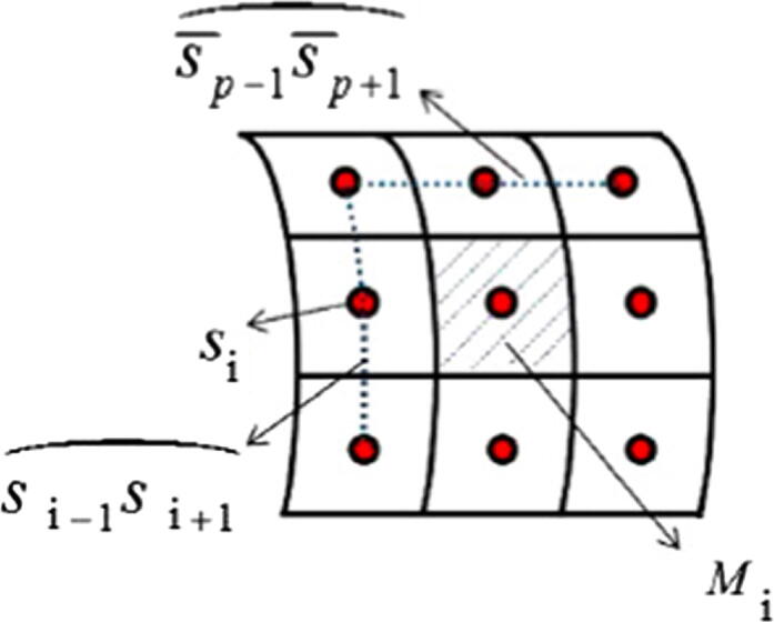
The schematic diagram of the source points $s_i$ and corresponding infinitesimal area $M_i$ on 3D problems.

Numerical implementation

The numerical results obtained by the proposed meshless approach are presented on several test problems with various geometries. We consider three diverse benchmark problems are thus chosen to illustrate the reliability and accuracy of the proposed meshless technics. Prime example of proposal approach devoted to a problem with constant order derivatives on an ellipsoidal domain, and the gained results are compared with the exact solutions to establish the validity of the proposed method. In the latter problem, a spherical domain is considered and the stability and accuracy proposal method is revealed and tabulated. The proposal meshless technics on the atmosphere surface is investigated for the last case. The analytical solution of the examples is given as a comparison with the SBM-DRM solution. To perceive the accuracy of the presented meshless method, and relative $L_2$ norm errors are exploited. The discrete relative $L_2$ norm of error is deemed as:

Relative $L_2$ error norm: $\frac{\Vert u-\tilde{u}\Vert }{\Vert u\Vert }\simeq \sqrt{\frac{{\sum }_{i,j=1}^{N_t}{\left(u\right(x_i,t_j)-\tilde{u}(x_i,t_j\left)\right)}^2}{{\sum }_{i=1}^{N_t}{u}^2(x_i,t_j)}}$, where, $N_t$ is the number of test points. As well, $\tilde{u}(x_i,t_j)$ and $u(x_i,t_j)$ respectively represent the analytical and numerical results evaluated at $(x_i,t_j)$.

Example 0.1

Let domain $\mathrm{\Omega }$ be ellipsoidal with the following parameter equation

$$x=3\sin \left(\varphi \right)\cos \left(\theta \right),y=2\sin \left(\varphi \right)\sin \left(\theta \right),z=\cos \left(\varphi \right),\theta \in [0,2\pi ],\varphi \in [0,\pi ]\text{.}$$ (26)

The Eq. (1) is considered with $A=1,\mu =1$, and the initial condition:

$$u(x,y,z,t=0)=0,(x,y,z)\in \mathrm{\Omega },$$ (27)

the Dirichlet boundary condition is

$$u(x,y,z,t)=t^3\left[x\right(2-x)+y(2-y)+z(2-z\left)\right],(x,y,z)\in \partial \mathrm{\Omega },$$ (28)

Moreover, the right hand side function is

$$f(x,y,z,t)=(\frac{6}{\mathrm{\Gamma }(4-\alpha )}{t}^{3-\alpha }+t^3)\left[x\right(2-x)+y(2-y)+z(2-z\left)\right]+6t^3\text{.}$$ (29)

The analytical solution of the problem is given by

$$u(x,y,z,t)=t^3\left[x\right(2-x)+y(2-y)+z(2-z\left)\right]\text{.}$$ (30)

Fig. 2 shows the geometry of the problem. The outer surface of the ellipsoid and an inner test surface with radius $0.6$ and related nodal distribution are also illustrated where the blue dots are the boundary source points and the dark dots are the inner points. To investigate the performance of the present method, 3500 test points are totally selected within the ellipsoid. The test points are also distributed on 10 ellipsoids with the radius 0.1 to 1 and 350 points are selected on each one. Table 2, Table 3 give the relative error norm using the RBF formulation respectively with $p=8$ and $p=10$ for different $\alpha$ ($0.1,0.5,0.9$) with varying temporal step sizes $\delta t$ (0.02,0.01,0.005) and varying the total number of collocation points $n=M+N$ $(320,405,500)$. Parameters M and N also determine the number of inner and source points; receptively. It can be observed that the SBM-DRM solutions are more accurate as the number of collocation points increases. It is also noted that the numerical accuracy rises following the reduction in time levels. Comparing the results of Table 2, Table 3 reveals that better accuracy is achieved once the order of poly-harmonic splines p is higher. Moreover, the smaller fractional order $\alpha$ yields higher accuracy as mentioned in the results.

Fig. 2.

Consider outer and inner surfaces of ellipsoidal with related nodal distribution (boundary source points and inner points).

Table 2.

Numerical result of $L_2$ norm errors in diverse $\alpha$ and diverse sets of collocation nodes(Example 0.1).

		$\delta t$		RBF with $p=8$
				$n=320$		$n=405$		$n=500$
$\alpha =0.1$		0.02		$8.771911\times {10}^{-5}$		$4.825727\times {10}^{-5}$		$2.892057\times {10}^{-5}$
		0.01		$4.670724\times {10}^{-5}$		$2.716776\times {10}^{-5}$		$2.229224\times {10}^{-5}$
		0.005		$4.621369\times {10}^{-5}$		$2.665169\times {10}^{-5}$		$2.168148\times {10}^{-5}$
$\alpha =0.5$		0.02		$1.089088\times {10}^{-4}$		$9.695786\times {10}^{-5}$		$8.984681\times {10}^{-5}$
		0.01		$6.191015\times {10}^{-5}$		$4.779506\times {10}^{-5}$		$3.977905\times {10}^{-5}$
		0.005		$4.692587\times {10}^{-5}$		$3.112011\times {10}^{-5}$		$2.233062\times {10}^{-5}$
$\alpha =0.9$		0.02		$7.562059\times {10}^{-4}$		$7.471623\times {10}^{-4}$		$7.408496\times {10}^{-4}$
		0.01		$3.718842\times {10}^{-4}$		$3.616689\times {10}^{-4}$		$3.547111\times {10}^{-4}$
		0.005		$1.896697\times {10}^{-4}$		$1.782153\times {10}^{-4}$		$1.707275\times {10}^{-4}$

Table 3.

Numerical result of $L_2$ norm errors in diverse $\alpha$ and diverse sets of collocation nodes(Example 0.1).

		$\delta t$		RBF with $p=10$
				$n=320$		$n=405$		$n=500$
$\alpha =0.1$		0.02		$2.386586\times {10}^{-5}$		$1.651131\times {10}^{-5}$		$7.732672\times {10}^{-6}$
		0.01		$1.599791\times {10}^{-5}$		$1.080011\times {10}^{-5}$		$7.221327\times {10}^{-6}$
		0.005		$1.448835\times {10}^{-5}$		$1.027734\times {10}^{-5}$		$5.827354\times {10}^{-6}$
$\alpha =0.5$		0.02		$7.469885\times {10}^{-5}$		$7.253636\times {10}^{-5}$		$6.933223\times {10}^{-5}$
		0.01		$2.407584\times {10}^{-5}$		$2.193824\times {10}^{-5}$		$2.003451\times {10}^{-5}$
		0.005		$1.176374\times {10}^{-5}$		$7.233034\times {10}^{-6}$		$6.664477\times {10}^{-6}$
$\alpha =0.9$		0.02		$7.284190\times {10}^{-4}$		$7.259831\times {10}^{-4}$		$7.226772\times {10}^{-4}$
		0.01		$3.425191\times {10}^{-4}$		$3.399368\times {10}^{-4}$		$3.367779\times {10}^{-4}$
		0.005		$1.585369\times {10}^{-4}$		$1.558087\times {10}^{-4}$		$1.528928\times {10}^{-4}$

For further investigation, in Fig. 3, the absolute errors of the SBM-DRM method are computed on the outer surface of the ellipsoid using the poly-harmonic splines of order 10 with fixed $\alpha =0.5$ and $n=405$, and different temporal step sizes at final time $t=1$. In Fig. 4, Fig. 5, the absolute errors are additionally computed on the test inner surface in Fig. 2 at different time levels $t=0.2,t=0.5$ and $t=1$ using the RBFs with $p=10,\delta t=0.01$ and $n=405$ in which 310 inner nodes are used. It is evidently obvious that the numerical results provide superb agreement with accuracy in the ellipsoidal domain.

Example 0.2

As a second example, the VO-FDE is considered in a peanut domain, where the Dirichlet boundary condition is specified on the whole surface. The initial and the boundary conditions are also defined as follows:

$$u(x,y,z,t=0)=0,(x,y,z)\in \mathrm{\Omega },$$ (31)

$$u(x,y,z)=t^3{e}^{x+y+z},(x,y,z)\in \partial \mathrm{\Omega },$$

and the function $f(x,y,z,t)$ and the analytical solution are given by

$$f(x,y,z,t)=[\frac{6}{\mathrm{\Gamma }(4-\alpha (t\left)\right)}{t}^{3-\alpha \left(t\right)}-3t^3]e^{x+y+z}\text{.}$$ (32)

$$u(x,y,z,t)=t^3{e}^{x+y+z},$$ (33)

where $\alpha \left(t\right)=0.8+0.2t/T$. The parameter equation of the peanut surface is given by

$$x=\rho \left(\theta \right)\cos \left(\theta \right),y=\rho \left(\theta \right)\sin \left(\theta \right)\sin \left(\varphi \right),z=\rho \left(\theta \right)\sin \left(\theta \right)\cos \left(\varphi \right),$$ (34)

in which $\varphi \in [0,\pi ]$ is angle between positive x-axis and the position vector $r=(x,y,z)$, and $\theta \in [0,2\pi ]$ denotes angle between projection of r on plane Oyz and the positive y-axis. The length r is given by:

$$\rho \left(\theta \right)={\left(\cos \right(3\theta )+\sqrt{7-{\sin }^2\left(3\theta \right)})}^{\frac{1}{3}}\text{.}$$ (35)

Fig. 3.

Absolute error of SBM-DRM solution on outer surface of ellipsoidal domain ($p=10,n=405,t=1$).

Fig. 4.

Absolute error of SBM-DRM solution on inner surface of ellipsoidal domain ($p=10,n=400,\delta t=0.01$).

Fig. 5.

(Right) exact solution and (left) absolute error of SBM-DRM solution on inner surface of ellipsoidal domain ($p=10,n=400$, $\delta t=0.01$).

Fig. 6 shows the geometry of this problem where the blue nodes are the boundary source nodes. Similar to the last example, 3500 test points within the peanut domain are totally chosen. The test points are selected on 10 peanuts with the radius $0.1$ to 1 of the radius of the main peanut whereas 350 points are selected on each one. Table 4, Table 5 give the relative error norm using the RBF formulation with $p=4$ and $p=6$ in Table 4 and $p=8$ and $p=10$ in Table 5, for constant $\alpha =0.5$ with varying temporal step sizes $\delta t$ (0.02,0.01,0.005) and varying the total number of collocation points $n=M+N$ $(320,500)$. It can be observed that the SBM-DRM solutions are more accurate as the number of collocation nodes increases. It can be also detected that the numerical accuracy raises upon the decline in time levels. Comparing the results of Table 4, Table 5 demonstrates that better accuracy is achieved when the order of poly-harmonic splines p is higher.

Fig. 6.

Surface of the peanut with related nodal distributions in Example 0.2.

Table 4.

Numerical result of $L_2$ norm errors in diverse time levels and diverse sets of collocation nodes on domain (Example 0.2).

		$\delta t$		$p=4$				$p=6$
				$n=320$		$n=500$		$n=320$		$n=500$
$\alpha =0.5$		0.02		$9.230572\times {10}^{-3}$		$6.019641\times {10}^{-3}$		$7.805276\times {10}^{-4}$		$6.518941\times {10}^{-4}$
		0.01		$5.080682\times {10}^{-3}$		$2.371643\times {10}^{-3}$		$6.956351\times {10}^{-4}$		$4.622802\times {10}^{-4}$
		0.005		$3.314679\times {10}^{-3}$		$9.025428\times {10}^{-4}$		$6.679885\times {10}^{-4}$		$2.7453441\times {10}^{-5}$

Table 5.

Numerical result of $L_2$ norm errors in diverse time levels and diverse sets of collocation nodes(Example 0.2).

		$\delta t$		$p=8$				$p=10$
				$n=320$		$n=500$		$n=320$		$n=500$
$\alpha =0.5$		0.02		$8.774479\times {10}^{-4}$		$4.286657\times {10}^{-4}$		$9.609672\times {10}^{-5}$		$7.108031\times {10}^{-5}$
		0.01		$3.080682\times {10}^{-4}$		$1.042351\times {10}^{-4}$		$8.766561\times {10}^{-5}$		$4.622802\times {10}^{-5}$
		0.005		$1.941911\times {10}^{-4}$		$8.766560\times {10}^{-5}$		$7.469885\times {10}^{-5}$		$1.555707\times {10}^{-6}$

Base on in Fig. 7, the absolute errors of the SBM-DRM method are computed on the outer surface of the peanut using poly-harmonic splines of order 7 and 9 with fixed $\alpha =0.5$ and $n=500$, and temporal step sizes $\delta t=0.005$ at final time $t=1$. Similarly, in Fig. 8, the absolute errors are computed on a test inner surface by using different poly-harmonic splines of order $p=8$ and $p=10$ with $\delta t=0.005$ at time $t=1$ and $n=500$ in which 310 inner nodes and 190 boundary source nodes are used. It is evidently obvious that the numerical results provide good agreement with accuracy in this peanut domain. In addition, a testing rectangular plane is taken within the peanut as $\left\{(x,y,z)\mid x\in [-0.8,0.8],y\in [-0.2,0.2],z=0\right\}$. The relative error of the SBM-DRM on this plane is calculated and illustrated in Fig. 9. It is observed that the error decreases as more collocation points are applied on the plane.

Example 0.3

Consider Eq. (1) with $A=1,\mu =0$ on complex geometry, zero initial condition, along with the following boundary condition is considered:

$$u(x,y,z)=t^3\sin \left(\frac{\pi }{2}x\right)\sin \left(\frac{\pi }{2}y\right)\sin \left(\frac{\pi }{2}z\right),(x,y,z)\in \partial \mathrm{\Omega },$$ (36)

where $f(x,y,z,t)=[\frac{6}{\mathrm{\Gamma }(4-\alpha )}{t}^{3-\alpha }+\frac{3{\pi }^2}{4}{t}^3]\sin \left(\frac{\pi }{2}x\right)\sin \left(\frac{\pi }{2}y\right)\sin \left(\frac{\pi }{2}z\right)$ and the exact solution is

$$u(x,y,z)=t^3\sin \left(\frac{\pi }{2}x\right)\sin \left(\frac{\pi }{2}y\right)\sin \left(\frac{\pi }{2}z\right)\text{.}$$ (37)

Fig. 10 shows the geometry of the domain which is defined parametrically as

$$x=\rho \left(\varphi \right)\cos \left(\varphi \right),y=\rho \left(\varphi \right)\sin \left(\varphi \right)\cos \left(\theta \right),z=\rho \left(\varphi \right)\sin \left(\varphi \right)\sin \left(\theta \right),\varphi \in [0,\pi ],\theta \in [0,2\pi ],$$ (38)

where

$$\rho \left(\varphi \right)=\sqrt{\cos \left(2\varphi \right)+\sqrt{1.1-{\sin }^2\left(2\varphi \right)}}\text{.}$$ (39)

Fig. 7.

Absolute error of the SBM-DRM solution on outer surface of the domain ($\mathrm{\Delta }t$ = 0.005, n = 500, t = 1).

Fig. 8.

Graphs bsolute error of SBM-DRM solution on outer surface of ellipsoidal domain ($\delta t$ = 0.005, n = 500, t = 1).

Fig. 9.

Relative error of SBM-DRM solution on rectangular domain within peanut as $\left\{(x,y,z)\mid x\in [-0.8,0.8],y\in [-0.2,0.2],z=0\right\}$ with $p=8$ and $\delta t=0.01$ in Example 0.2.

Fig. 10.

Considered computational domain with related nodal distributions in Example 0.3.

Similar to the previous example, 3500 test points are totally distributed within the computational domain to investigate the performance of the present method. Table 6 compares the relative error norm of the numerical solution derived using the RBF formulation of order $p=8$ and $p=10$ with varying the total number of collocation points n$n=M+N$ $(405,500,720)$. The time step is taken as $\delta t=0.02,0.01$ and $0.005$. The error is also found for the problem by different value of $\alpha$. In Table 6, the stability and accuracy proposal numerical approximation is tabulated. Further, the results demonstrate that better accuracy is achieved when the order of poly-harmonic splines p is higher. It is observed that the numerical accuracy is boosted with the decline of temporal sizes.

Table 6.

Numerical result of $L_2$ norm errors in diverse time levels and diverse sets of collocation nodes on domain (Example 0.3).

		$\delta t$		Fractional order $\alpha =0.5$
				$n=405$		$n=500$		$n=720$
$p=8$		0.02		$1.987401\times {10}^{-4}$		$1.302407\times {10}^{-4}$		$1.046461\times {10}^{-4}$
		0.01		$1.611973\times {10}^{-4}$		$1.152006\times {10}^{-4}$		$9.809952\times {10}^{-5}$
		0.005		$1.567420\times {10}^{-4}$		$1.028890\times {10}^{-4}$		$9.599854\times {10}^{-5}$
$p=10$		0.02		$9.586725\times {10}^{-5}$		$9.015915\times {10}^{-5}$		$8.414206\times {10}^{-5}$
		0.01		$9.235362\times {10}^{-5}$		$8.620175\times {10}^{-5}$		$8.332679\times {10}^{-5}$
		0.005		$8.933214\times {10}^{-5}$		$8.476604\times {10}^{-5}$		$7.999854\times {10}^{-5}$

As one can see, a testing surfaces whose radius is half of the main radius is selected (39). Fig. 11, Fig. 12 illustrate a comparison of the absolute errors on this test inner surface achieved by a various number of collocation nodes $n=405$, $n=500$ and $n=720$, exploiting the RBF formulation of order $p=10$. The time step is also given as $\delta t=0.005$ and the errors are computed at the final time $t=1$. It is evidently obvious that the numerical results provide great agreement with accuracy in the irregular computational domain. It is also spotted that the accuracy improves following the increase in the number of collocation points.

Fig. 11.

Absolute error of the numerical solution on inner surface of the domain ($\delta t$ = 0.005, $p=8,t=1$).

Fig. 12.

Exact solution and absolute error of the SBM-DRM solution on inner surface of the domain ($\delta t$ = 0.005, $p=8$, $t=1$).

Conclusion

In this paper, a meshless RBF-based SBM/DRM was developed to simulate three-dimensional variable-order time fractional diffusion equations. The proposed method was successfully applied on 3-D arbitrary domains of the numerical examples with Dirichlet boundary conditions. The proposed scheme are shown to be easy to implement, integration-free, straightforward, mathematically simple, easy to implement, highly accurate and truly meshless. The interpolation method The proposal meshless method as truly meshless approach dose not require predefined cell or background integration mesh in computational domain. The time fractional derivative is addressed in Caputao sense. The point interpolation method with the help of RBF has been proposed to contract shape function which have satisfied Kronecker function property. We have used the finite difference scheme for discretizing the time dime direction then a meshless strong formulation used to solved the sim-discretized problem proposed on surface. The present numerical examples show that the SBM-DRM is a competitive meshless collocation method for $3D$ VO-TFDEs and provides satisfactory solutions with high accuracy. Furthermore, numerical experiments verify that the SBM-DRM is sensitive to some parameters such as the order of the RBF formulation, time step, and number of collocation nodes. So that, in most cases, higher order RBFs, decrement in time steps, and increment of number of interpolation nodes can lead to better accuracy.

Declaration of Competing Interest

The author declare that they have no conflict of interest.

Compliance with Ethics Requirements

This article does not contain any studies with human or animal subjects.

Funding

Not applicable.

References

- 1.Alotta G., Barrera O., Cocks A.C.F., Di Paola M. On the behavior of a three-dimensional fractional viscoelastic constitutive model. Meccanica. 2017;52:2127–2142. [Google Scholar]
- 2.Amblard F., Maggs A.C., Yurke B., Pargellis A.N., Leibler S. Subdiffusion and anomalous local viscoelasticity in actin networks. Phys Rev Lett. 1996;77:4470. doi: 10.1103/PhysRevLett.77.4470. [DOI] [PubMed] [Google Scholar]
- 3.Babaei A., Jafari H., Ahmadi M. A fractional order HIV/AIDS model based on the effect of screening of unaware infectives. Math Methods Appl Sci. 2019;42:2334–2343. [Google Scholar]
- 4.Baleanu D., Ghanbari B., Asad J.H., Jajarmi A., Pirouz H.M. Planar system-masses in an equilateral triangle: numerical study within fractional calculus. CMES-Comput Model Eng Sci. 2020;124:953–968. [Google Scholar]
- 5.Baleanu D., Jajarmi A., Sajjadi S.S., Asad J.H. The fractional features of a harmonic oscillator with position-dependent mass. Commun Theor Phys. 2020;72:55002. [Google Scholar]
- 6.Baleanu D, Sweilam NH, AL-Mekhlafi SM, Alshomrani AS. Comparative study for optimal control nonlinear variable-order fractional tumor model; 2020.
- 7.Blumen A., Zumofen G., Klafter J. Transport aspects in anomalous diffusion: Lévy walks. Phys Rev A. 1989;40:3964. doi: 10.1103/physreva.40.3964. [DOI] [PubMed] [Google Scholar]
- 8.Chen C.M., Liu F., Turner I., Anh V. A Fourier method for the fractional diffusion equation describing sub-diffusion. J Comput Phys. 2007;227:886–897. [Google Scholar]
- 9.Chen W., Gu Y. An improved formulation of singular boundary method. Adv Appl Math Mech. 2012;4:543–558. [Google Scholar]
- 10.Chen W., Wang F. Singular boundary method using time-dependent fundamental solution for transient diffusion problems. Eng Anal Bound Elem. 2016;68:115–123. [Google Scholar]
- 11.Chen W., Zhang J.Y., Fu Z.J. Singular boundary method for modified Helmholtz equations. Eng Anal Bound Elem. 2014;44:112–119. [Google Scholar]
- 12.Coimbra C.F.M. Mechanics with variable-order differential operators. Ann Phys. 2003;12:692–703. [Google Scholar]
- 13.Cui M. Compact finite difference method for the fractional diffusion equation. J Comput Phys. 2009;228:7792–7804. [Google Scholar]
- 14.Din A., Khan A., Baleanu D. Stationary distribution and extinction of stochastic coronavirus (COVID-19) epidemic model. Chaos, Solitons Fract. 2020;139:110036. doi: 10.1016/j.chaos.2020.110036. [DOI] [PMC free article] [PubMed] [Google Scholar]
- 15.Domanov Y.A., Aimon S., Toombes G.E.S., Renner M., Quemeneur F., Triller A., Turner M.S., Bassereau P. Mobility in geometrically confined membranes. Proc Nat Acad Sci. 2011;108:12605–12610. doi: 10.1073/pnas.1102646108. [DOI] [PMC free article] [PubMed] [Google Scholar]
- 16.Dou F., Hon Y. Kernel-based approximation for Cauchy problem of the time-fractional diffusion equation. Eng Anal Bound Elem. 2012;36:1344–1352. [Google Scholar]
- 17.Fu Z.J., Chen W., Gu Y. Burton–Miller-type singular boundary method for acoustic radiation and scattering. J Sound Vib. 2014;333:3776–3793. [Google Scholar]
- 18.Gao G.h., Sun Z.z. A compact finite difference scheme for the fractional sub-diffusion equations. J Comput Phys. 2011;230:586–595. [Google Scholar]
- 19.Gao W., Baskonus H.M., Shi L. New investigation of bats-hosts-reservoir-people coronavirus model and application to 2019-nCoV system. Adv Difference Eq. 2020;2020:1–11. doi: 10.1186/s13662-020-02831-6. [DOI] [PMC free article] [PubMed] [Google Scholar]
- 20.Gao W, Veeresha P, Baskonus HM, Prakasha DG, Kumar P. A new study of unreported cases of 2019-nCOV Epidemic Outbreaks. Chaos, Solitons & Fractals; 2020b, 109929. [DOI] [PMC free article] [PubMed]
- 21.Gao W., Veeresha P., Prakasha D.G., Baskonus H.M. New numerical simulation for fractional Benney-Lin equation arising in falling film problems using two novel techniques. Numer Methods Partial Diff Eqs. 2020;37:210–243. [Google Scholar]
- 22.Gao W., Yel G., Baskonus H.M., Cattani C. Complex solitons in the conformable (2+ 1)-dimensional Ablowitz-Kaup-Newell-Segur equation. Aims Math. 2020;5:507–521. [Google Scholar]
- 23.Hermans E., Bhamla M.S., Kao P., Fuller G.G., Vermant J. Lung surfactants and different contributions to thin film stability. Soft Matter. 2015;11:8048–8057. doi: 10.1039/c5sm01603g. [DOI] [PubMed] [Google Scholar]
- 24.Heydari M.H., Hooshmandasl M.R., Mohammadi F. Legendre wavelets method for solving fractional partial differential equations with Dirichlet boundary conditions. Appl Math Comput. 2014;234:267–276. [Google Scholar]
- 25.Hosseini V.R., Chen W., Avazzadeh Z. Numerical solution of fractional telegraph equation by using radial basis functions. Eng Anal Bound Elem. 2014;38:31–39. [Google Scholar]
- 26.Hosseini V.R., Shivanian E., Chen W. Local integration of 2-D fractional telegraph equation via local radial point interpolant approximation. Eur Phys J Plus. 2015;130:1–21. [Google Scholar]
- 27.Hosseini V.R., Shivanian E., Chen W. Local radial point interpolation (MLRPI) method for solving time fractional diffusion-wave equation with damping. J Comput Phys. 2016;312:307–332. [Google Scholar]
- 28.Jafari H., Sadeghi J., Safari F., Kubeka A. Factorization method for fractional Schrödinger equation in D-dimensional fractional space and homogeneous manifold SL (2, c)/GL (1, c) Comput Methods Diff Eqs. 2019;7:199–205. [Google Scholar]
- 29.Jajarmi A., Baleanu D. On the fractional optimal control problems with a general derivative operator. Asian J Control. 2019 [Google Scholar]
- 30.Jajarmi A., Baleanu D. A new iterative method for the numerical solution of high-order non-linear fractional boundary value problems. Front Phys. 2020;8:220. [Google Scholar]
- 31.Jajarmi A., Yusuf A., Baleanu D., Inc M. A new fractional HRSV model and its optimal control: a non-singular operator approach. Physica A. 2020;547:123860. [Google Scholar]
- 32.Jiang Y., Ma J. High-order finite element methods for time-fractional partial differential equations. J Comput Appl Math. 2011;235:3285–3290. [Google Scholar]
- 33.Katsikadelis J.T. The BEM for numerical solution of partial fractional differential equations. Comput Math Appl. 2011;62:891–901. [Google Scholar]
- 34.Kumar P., Kumar S., Raman B. A fractional order variational model for the robust estimation of optical flow from image sequences. Optik. 2016;127:8710–8727. [Google Scholar]
- 35.Kumar S., Kumar D., Singh J. Fractional modelling arising in unidirectional propagation of long waves in dispersive media. Adv Nonlinear Anal. 2016;5:383–394. [Google Scholar]
- 36.Kumar S., Kumar R., Singh J., Nisar K.S., Kumar D. An efficient numerical scheme for fractional model of HIV-1 infection of CD4+ T-cells with the effect of antiviral drug therapy. Alexandria Eng J. 2020 [Google Scholar]
- 37.Kupradze V.D., Aleksidze M.A. The method of functional equations for the approximate solution of certain boundary value problems. USSR Comput Math Math Phys. 1964;4:82–126. [Google Scholar]
- 38.Makris N. Three-dimensional constitutive viscoelastic laws with fractional order time derivatives. J Rheol. 1997;41:1007–1020. [Google Scholar]
- 39.Mohammadi F., Moradi L., Baleanu D., Jajarmi A. A hybrid functions numerical scheme for fractional optimal control problems: application to nonanalytic dynamic systems. J Vib Control. 2018;24:5030–5043. [Google Scholar]
- 40.Muleshkov A.S., Golberg M.A., Chen C.S. Particular solutions of Helmholtz-type operators using higher order polyhrmonic splines. Comput Mech. 1999;23:411–419. [Google Scholar]
- 41.Naik P.A., Yavuz M., Qureshi S., Zu J., Townley S. Modeling and analysis of COVID-19 epidemics with treatment in fractional derivatives using real data from Pakistan. Eur Phys J Plus. 2020;135:1–42. doi: 10.1140/epjp/s13360-020-00819-5. [DOI] [PMC free article] [PubMed] [Google Scholar]
- 42.Nardini D., Brebbia C.A. A new approach to free vibration analysis using boundary elements. Appl Math Model. 1983;7:157–162. [Google Scholar]
- 43.Owolabi K.M. Mathematical analysis and numerical simulation of chaotic noninteger order differential systems with Riemann-Liouville derivative. Prog Fraction Diff Appl. 2020;6:29–42. [Google Scholar]
- 44.Pinto C.M.A., Carvalho A.R.M., Tavares J.N. Time-varying pharmacodynamics in a simple non-integer HIV infection model. Math Biosci. 2019;307:1–12. doi: 10.1016/j.mbs.2018.11.001. [DOI] [PubMed] [Google Scholar]
- 45.Podlubny I. volume 198. Academic press; 1998. (Fractional differential equations: an introduction to fractional derivatives, fractional differential equations, to methods of their solution and some of their applications). [Google Scholar]
- 46.Qureshi S., Atangana A. Fractal-fractional differentiation for the modeling and mathematical analysis of nonlinear diarrhea transmission dynamics under the use of real data. Chaos, Solitons Fract. 2020;136:109812. [Google Scholar]
- 47.Qureshi S., Chang M., Shaikh A.A. Analysis of series RL and RC circuits with time-invariant source using truncated M, atangana beta and conformable derivatives. J Ocean Eng Sci. 2020 [Google Scholar]
- 48.Rocha D., Gouveia S., Pinto C., Scotto M., Tavares J.N., Valadas E., Caldeira L.F. On the parameters estimation of HIV dynamic models. REVSTAT–Stat J. 2019;17:209–222. [Google Scholar]
- 49.Roscani S.D., Venturato L., Tarzia D.A. Global solution to a nonlinear fractional differential equation for the caputo-fabrizio derivative. Prog Fractional Diff Appl. 2019;5:269–281. [Google Scholar]
- 50.Sajjadi S.S., Baleanu D., Jajarmi A., Pirouz H.M. A new adaptive synchronization and hyperchaos control of a biological snap oscillator. Chaos, Solitons & Fract. 2020;138:109919. [Google Scholar]
- 51.Shivanian E. Analysis of meshless local radial point interpolation (MLRPI) on a nonlinear partial integro-differential equation arising in population dynamics. Eng Anal Bound Elem. 2013;37:1693–1702. [Google Scholar]
- 52.Shivanian E. A new spectral meshless radial point interpolation (SMRPI) method: a well-behaved alternative to the meshless weak forms. Eng Anal Bound Elem. 2015;54:1–12. [Google Scholar]
- 53.Shivanian E., Jafarabadi A. An improved meshless method for solving two-and three-dimensional coupled Klein–Gordon–Schrödinger equations on scattered data of general-shaped domains. Eng Comput. 2018;34:757–774. [Google Scholar]
- 54.Srivastava H.M., Dubey V.P., Kumar R., Singh J., Kumar D., Baleanu D. An efficient computational approach for a fractional-order biological population model with carrying capacity. Chaos, Solitons & Fractals. 2020;138:109880. [Google Scholar]
- 55.Sun H., Chen W., Chen Y. Variable-order fractional differential operators in anomalous diffusion modeling. Physica A. 2009;388:4586–4592. [Google Scholar]
- 56.Sun H.G., Chen W., Wei H., Chen Y.Q. A comparative study of constant-order and variable-order fractional models in characterizing memory property of systems. Eur Phys J Special Top. 2011;193:185. [Google Scholar]
- 57.Sweilam N.H., Abou Hasan M.M. An Improved Method for Nonlinear Variable - Order Lévy - Feller Advection-Dispersion Equation. Bull Malays Math Sci Soc. 2019;42:3021–3046. [Google Scholar]
- 58.Sweilam N.H., Al-Mekhlafi S.M., Shatta S.A., Baleanu D. Numerical study for two types variable-order Burgers’ equations with proportional delay. Appl Numer Math. 2020 [Google Scholar]
- 59.Wang L., Zheng H., Lu X., Shi L. A Petrov-Galerkin finite element interface method for interface problems with Bloch-periodic boundary conditions and its application in phononic crystals. J Comput Phys. 2019;393:117–138. [Google Scholar]
- 60.Yao G., Chen C., Zheng H. A modified method of approximate particular solutions for solving linear and nonlinear PDEs. Numer Methods Partial Differential Eqs. 2017;33:1839–1858. [Google Scholar]
- 61.Yin C., Cheng Y., Chen Y., Stark B., Zhong S. Adaptive fractional-order switching-type control method design for 3D fractional-order nonlinear systems. Nonlinear Dyn. 2015;82:39–52. [Google Scholar]
- 62.Zheng H., Yang Z., Zhang C., Tyrer M. A local radial basis function collocation method10 for band structure computation of phononic crystals with scatterers of arbitrary geometry. Appl Math Model. 2018;60:447–459. [Google Scholar]
- 63.Zheng H., Zhang C., Wang Y., Sladek J., Sladek V. A meshfree local RBF collocation method for anti-plane transverse elastic wave propagation analysis in 2D phononic crystals. J Comput Phys. 2016;305:997–1014. [Google Scholar]
- 64.Zheng H., Zhou C., Yan D.J., Wang Y.S., Zhang C. A meshless collocation method for band structure simulation of nanoscale phononic crystals based on nonlocal elasticity theory. J Comput Phys. 2020;408:109268. [Google Scholar]