Identification and utilization of genetic determinants of trait measurement errors in image-based, high-throughput phenotyping

Abstract

The accuracy of trait measurements greatly affects the quality of genetic analyses. During automated phenotyping, trait measurement errors, i.e. differences between automatically extracted trait values and ground truth, are often treated as random effects that can be controlled by increasing population sizes and/or replication number. In contrast, there is some evidence that trait measurement errors may be partially under genetic control. Consistent with this hypothesis, we observed substantial nonrandom, genetic contributions to trait measurement errors for five maize (Zea mays) tassel traits collected using an image-based phenotyping platform. The phenotyping accuracy varied according to whether a tassel exhibited “open” versus. “closed” branching architecture, which is itself under genetic control. Trait-associated SNPs (TASs) identified via genome-wide association studies (GWASs) conducted on five tassel traits that had been phenotyped both manually (i.e. ground truth) and via feature extraction from images exhibit little overlap. Furthermore, identification of TASs from GWASs conducted on the differences between the two values indicated that a fraction of measurement error is under genetic control. Similar results were obtained in a sorghum (Sorghum bicolor) plant height dataset, demonstrating that trait measurement error is genetically determined in multiple species and traits. Trait measurement bias cannot be controlled by increasing population size and/or replication number.

The accuracy of high-throughput phenotyping can be affected by genetically determined measurement biases, which can alter the results of genetic analyses.

Introduction

Genetic analyses (e.g. genome-wide association study [GWAS]) and the development of genomic selection models to facilitate breeding for quantitative traits typically require the genotyping and phenotyping of hundreds to thousands of individuals. Because advances in sequencing technology have enabled the quick and cost-effective genotyping of large numbers of individuals, phenotyping has become the bottleneck for such studies. To cope up with this challenge, multiple automated phenotyping strategies have been developed (Kircher and Kelso, 2010; Slatko et al., 2018; Ramstein et al., 2019). Among these strategies, image-based phenotyping is one of the most favored approaches in plants due to its low cost, ability to be deployed in both controlled environments and under field conditions, and the increased capabilities of computational and imaging devices, which have accelerated both the pace and precision of phenotyping (Araus and Cairns, 2014; Yang et al., 2017; Ramstein et al., 2019; Das Choudhury et al., 2019).

In conjunction with increased throughput, the expected increases in precision and repeatability from image-based phenotyping should theoretically enable more reliable inferences about causal loci and increase statistical power in genetic analysis (Ramstein et al., 2019). However, phenotypes collected via images are projections of 3D structures onto 2D planes and can therefore lose information due to occlusion and the angle from which an image is captured (Lobet et al., 2017; Zhou et al., 2019). This can cause trait values extracted from images to deviate from true phenotypic values. As a result, the accuracy of data collected from 2D images of 3D structures remains a challenge for all image-based phenotyping platforms. To overcome this issue, several studies have attempted to flatten objects prior to image collection to compress 3D structures into 2D structures to increase phenotyping accuracy (AL-Tam et al., 2013; Crowell et al., 2014; Vasseur et al., 2018). However, these methods can only be applied to objects that are flexible enough, such as seedlings or rice (Oryza sativa) panicles, to be flattened without damaging or altering the structures of interest. Of course, flattening 3D objects also results in the loss of structural information. Other studies have focused on imaging from multiple angles to reconstruct the 3D structure of plants or plant organs (McCormick et al., 2016; He et al., 2017; Li et al., 2020; Gaillard et al., 2020). However, the complexity of these methods generally restricts them to imaging in controlled environments rather than under field conditions. Although encouraging progress on phenotyping plant height, flowering time, and plant stress under field conditions via unmanned aerial vehicles and robotic ground systems (Holman et al., 2016; Salas Fernandez et al., 2017; Ghosal et al., 2018; Anderson et al., 2019; Wu et al., 2019) has been achieved, for most agronomically important traits, it remains challenging to identify high-accuracy phenotyping solutions. Thus, trait measurement errors—the difference between automatically extracted trait measurements and true phenotypic values (i.e. ground truth)—are expected in data sets generated by high-throughput phenotyping platforms, and these errors can potentially affect the results of genetic analyses.

For genetic analyses using linear models, tests of significance are mainly affected by population size, the magnitude of estimated allelic effects, and the residual error variance (Wang and Xu, 2019). Therefore, trait measurement errors, which can cause inaccurate estimation of allelic effects and increase residual variance, reduce statistical power. It is commonly assumed that the typically lower heritabilities exhibited by phenotypes from image-based high-throughput phenotyping platforms as compared to manually measured phenotypes (Gage et al., 2017; Salas Fernandez et al., 2017) are a consequence of imprecise measurements inflating the residual variance and that consequently the use of large populations would have the potential to offset losses in statistical power due to the imprecision of automated phenotyping (Gage et al., 2018a). Under these assumptions, the automatically and manually measured phenotypes are different representations of the same underlying trait (i.e. the genetic effects are identical). However, this line of reasoning relies on the assumption that the sources of trait measurement errors are random, nongenetic factors. In contrast, a recent study compared biomass estimated via RGB imaging to measured biomass weights and reported systematic differences in the error distributions for different genotypes (Liang et al., 2018). Similarly, Lobet et al. (2017) found that phenotyping accuracy from root images varied according to root type and decreased as root size increased. These studies shed light on an issue that has been largely ignored in the scientific literature: the possibility that automated phenotyping biases arising via interactions between genotypes and phenotyping methods can introduce spurious associations between genetic markers and trait values automatically extracted from images.

The male inflorescence, or tassel, of maize (Zea mays) is located at the apex of the mature plant with flower-bearing branches that grow sequentially from the main axis and extend in different directions. Structural characteristics of maize tassels are highly heritable (Schuetz and Mock, 1978; Brown et al., 2011) and appear to have experienced indirect selection, potentially due to their roles in hybrid seed production (Duvick and Cassman, 1999; Duvick, 2005; Gage et al., 2018b). This has driven an interest in developing and deploying field-based high-throughput phenotyping platforms for tassels. However, the branches of maize tassels usually grow in an asymmetric manner such that one branch can easily be occluded by another (Vollbrecht and Schmidt, 2009). This growth pattern makes it challenging to develop accurate feature extraction pipelines for tassel images. Consequently, most studies of tassel morphology focus primarily on tassel length and weight—traits that are less likely to be affected by occluded branches. Methods for collecting other important traits, such as central spike length, branch length, branch number, and branch angles, have been hampered by difficulties in the automatic identification of branching points from 2D images (Gage et al., 2017). These morphological features make the maize tassel a good model to test our hypothesis that interactions between morphological traits and phenotyping platforms can influence the outcomes of genetic analyses.

In this study, we constructed a computational pipeline, Tassel Image-Trait Extraction Tool (TI-TET), to semi-automatically extract traits from images of maize tassels and tested this pipeline using a diverse panel of maize inbreds. We then evaluated the magnitude of trait measurement errors, as measured by the differences between trait values extracted from images using TI-TET, and manually measured trait values from the same tassels for tassels with differing levels of structural complexity. We found that trait measurement errors have genetic components, which were validated by identifying associations between candidate genes that altered tassel structure and trait measurement errors. We also extended and confirmed these results by conducting a similar analysis for automated phenotyping and manual measurements of plant height in the sorghum (Sorghum bicolor) association panel (SAP). Our findings demonstrate that substantial amounts of genetic variation underlie trait measurement errors, which raises issues for the design of phenotyping projects.

Results

Trait extraction

We collected tassels from 339 inbred maize lines from the shoot apical meristem (SAM) diversity panel (Leiboff et al., 2015) and imaged each tassel from five imaging angles (Figure 1, “Methods” section). We then extracted five traits from the resulting images: tassel length, central spike length, branching zone length, lowest branch length, and lowest branch angle from the resulting images using our semi-automated trait extraction pipeline, TI-TET (see Supplemental Protocol). The same traits were measured manually on each tassel. Although it is likely impossible to ever measure traits without any error, we are confident that the manual tassel measurements generated in this study are highly accurate. They were all collected by a single individual indoors (thereby avoiding artifacts caused by variation in lighting) using standard protocols (see “Methods” section for further details). Consequently, we define the manual measurements as “ground truth” for assessing the accuracy of automated trait measurements.

Figure 1.

Imaging setup, procedure, and phenotypes. A, Tassel imaging platform. B, Schematic of the five views collected for each tassel. C, Five automatically collected tassel traits following image segmentation.

Extracted trait values were compared with manually collected ground truth trait values separately for each imaging angle (view1 to view5), the mean phenotype of the first and third views, and the mean trait value of all five views to evaluate TI-TET and test the impact of imaging angle on phenotyping accuracy. The squared Pearson correlation coefficient (r²) showed that image-based trait values were highly correlated with manual measurements for tassel length, central spike length, and branching zone length, whereas r² for lowest branch length and branch angle were lower (Figure 2A). The mean value of multiple views resulted in equal or greater concordance between TI-TET and ground truth measurements, as quantified via root mean square errors (RMSEs; Figure 2B). We then selected image-based descriptors that exhibited high r² and low RMSE, i.e. the mean phenotypes of all five views for tassel length, central spike length, and branching zone length and the mean phenotype of the first and third views for lowest branch length and angle for further analyses.

Figure 2.

Phenotyping accuracy of traits extracted from images using a single view (views 1 to 5), the mean phenotype from two views (views 1 and 3), and the mean phenotype from all five views. A, Accuracy was estimated using the square of the Pearson correlation coefficient (r²). B, Accuracy estimated using RMSE.

Tassel structure and its influence on phenotyping accuracy

Accurately extracting a trait from images relies on the successful identification of certain morphological features that define the trait. For example, whether or not the topmost branch node and lowest branch node can be detected largely determines the accuracy of the lengths of the central spike and lowest branch length. Thus, it should be easier to accurately determine tassel trait values from images of tassels with a few branches sparsely distributed along the rachis than to determine the same values from images of tassels with compact and/or complex branching architectures (Figure 3A). We hypothesized that this type of structural variation could contribute to the observed variation in phenotyping accuracy.

Figure 3.

Tassel structures that potentially alter phenotyping accuracy. A, Example of the complexity of tassel architecture. From left to right, tassel with both the lowest and topmost branch node clearly visible, tassel with either of the two nodes not visible, and tassel in which it is challenging to detect either node in any of the five views. B, Summary of tassel openness in the SAM diversity panel.

To test this hypothesis, we classified the tassel structures of 335/339 genotypes as being “open”, “partially open”, or “closed” based on whether the highest and lowest branch node points of multiple tassels of a given genotype could be clearly detected (Figure 3B; “Methods” section). Out of 335 scored genotypes, 104 were classified as “open,” 47 as “partially open”, and the remaining 184 as “closed”.

Within each of the three groups of tassel types, we calculated correlations between manual measurements and trait values extracted from images. For all five tassel traits, “closed” tassels exhibited the lowest accuracies (Figure 4, A–F; Supplemental Figure S1). Additionally, all traits except branch angle exhibited unequal phenotypic variances between “open” and “closed” tassels (Levene’s test, P <0.05). We defined trait measurement error as the difference between automatically extracted trait values and ground truth measurements from the same tassel.

Figure 4.

Phenotyping accuracy varies between “open” and “closed” tassel architecture. A–E, Comparison of ground truth and mean phenotype extracted from images using TI-TET. The solid lines denote identical measurements between the two methods. Genotypes are displayed in each dotplot chart, with 104 genotypes classified as “open” and 184 classified as “closed”. Results of the full population are displayed in Supplemental Figure S1. F, Accuracies were calculated within tassel openness classes.

Variation in trait measurement errors from high-throughput phenotyping platforms can be due to systematic under- or overestimation, variation in the magnitude of errors, or both, within and across structure groups. “Closed” tassels exhibited significantly larger errors (Student’s t test, P <0.05) for tassel length, central spike length, and branching zone length than “open” tassels (Figure 5;Supplemental Data Set S1). In addition to these three traits, differences were also observed in lowest branch length for the absolute values of the errors and lowest branch angle for the ratios of errors to ground truth measurements (Supplemental Figure S2 and Supplemental Data Set S1), suggesting that the magnitude of measurement errors can be affected by tassel architecture.

Figure 5.

Violin plots of trait measurement errors (difference between automated and ground truth measurements) stratified by tassel openness. Mean trait values are marked by dots. ns is P>0.05, *, and **** represent P > 0.05, P ≤ 0.05, and P ≤ 0.0001, respectively, from a Student’s t test (Supplemental Data Set S1).

For all five automatically extracted tassel traits, measurement errors of a given tassel trait were correlated with the ground truth value of that trait. More interestingly, measurement errors of all but one of these tassel traits were correlated with ground truth values of other tassel traits (Figure 6;Supplemental Data Set S1). For example, although ground truth measurements of branch angle are not significantly correlated with ground truth measurements of central spike length, they are significantly correlated with trait measurement errors of central spike length. Specifically, as branch angles increased, the accuracy of automated central spike measurements decreased. Similarly, while branch number is not significantly correlated with lowest branch angle ground truth, it is significantly correlated with branch angle error. In addition, we observed correlations between ground truth values and the absolute values of measurement errors for multiple tassel traits (Supplemental Figure S3 and Supplemental Data Set S1) that were novel compared to signed measurement errors (Figure 6). Hence, ground truth measurements of tassel traits can be correlated with both the magnitudes and directions of measurement errors of other tassel traits.

Figure 6.

Pearson correlation coefficients between ground truth values (.GT) and measurement errors (.error) for tassel traits. Comparisons among ground truth measurements are marked by a black rectangle. TL, tassel length; CS, central spike length; BZ, branching zone length; LBL, lowest branch length; BA, lowest branch angle; BN, branch number. *, **, and *** represent P ≤ 0.05, P ≤ 0.01, and P ≤ 0.001, respectively, using a Student’s t test (Supplemental Data Set S1).

Using backward elimination (“Methods” section), we constructed multiple regression models for trait measurement errors using ground truth phenotypes and tassel openness as predictors. These models explained 17%–40% of the variance in phenotypic measurement errors (Supplemental Table S1). Because tassel traits are highly heritable (Schuetz and Mock, 1978; Brown et al., 2011; Gage et al., 2018b, the observed correlations between ground truth measurements and measurement errors of other traits suggests the presence of genetic effects in trait measurement errors. This finding contradicts the assumption that trait measurement errors are caused entirely by random, nongenetic factors (Gage et al., 2018a). In the discussion below, we distinguish between measurement error per se and the component of measurement error that is under genetic control, which we will call genetically determined measurement bias (GDMB).

Genetic determinants of trait measurement errors

We conducted a GWAS for tassel structure in the SAM panel using FarmCPUpp (Liu et al., 2016; Kusmec and Schnable, 2018) with openness tassel architecture as the phenotype (“Methods” section) and identified three trait-associated SNPs (TASs; Figure 7A;Supplemental Figure S4). Consistent with previous GWAS (Brown et al., 2011; Wu et al., 2016; Xu et al., 2017), one of these TASs is located 10.8-kb upstream of the ramosa3 (ra3) gene on chromosome 7. The ra3 gene regulates inflorescence branch elongation and secondary branch initiation (Gallavotti et al., 2010; Satoh-Nagasawa et al., 2006), and ra3 mutants usually exhibit highly branched tassels (Supplemental Figure S5). A second TAS located on chromosome 8 is 26.7-kb downstream of BARREN INFLORESCENCE1 (Bif1; Figure 7A), a gene that regulates the initiation of secondary axillary meristems (Barazesh and McSteen, 2008). Mutations of bif1 result in greatly reduced branch numbers and a single elongated central spike (GalLi et al., 2015; Barazesh and McSteen, 2008). The identification of these two candidate genes supports the view that the trait “open” versus “closed” tassels, which affects the accuracy of automated trait measurements of tassel morphology, is itself genetically regulated by genes that contribute to tassel morphology.

Figure 7.

Manhattan plots for tassel openness and trait measurement errors for tassel length and central spike length. A–C, GWAS results for tassel openness, tassel length measurement errors, and central spike measurement errors. Blue vertical lines and labels mark the positions of candidate genes. Red horizontal lines mark local FDR cutoffs: −log₁₀ (0.05).

We then conducted GWAS on the trait measurement errors associated with five tassel traits. Multiple TASs (N = 43, Supplemental Data Set S2) were identified for each trait. The physical positions of these TASs were compared to 69 genes reported to alter inflorescence architecture in maize (Supplemental Data Set S3); two of these single-nucleotide polymorphisms (SNPs) were adjacent to known inflorescence genes (“Methods” section). A permutation test (P < 0.001) indicated that this degree of overlap is more than expected by chance. One TAS for tassel length measurement error was 53.5-kb downstream of the beared-ear1 (bde1) gene (Figure 7B;Supplemental Figure S4), which has been reported to alter tassel branch number (Thompson et al., 2009). A second TAS for central spike length measurement error was 54.8-kb upstream of the ligueless1 (lg1) gene (Figure 7C;Supplemental Figure S4). Lewis et al. (2014) reported that mutant alleles of lg1 condition extremely acute tassel branches angles compared to the wild-type. Our analysis of a family segregating 1:1 for heterozygotes (Figure 8, A and C) and homozygotes (Figure 8, B and E) of a lg1 mutant allele confirmed this report. In contrast to the “open” tassel architecture of heterozygous genotypes, homozygous lg1 mutants exhibited a “closed” tassel architecture (Figure 8, A, B, D, and F); the lowest and second-lowest tassel branch angles of homozygous lg1 mutant plants were significantly smaller than those observed in heterozygous controls (Figure 8G;Supplemental Data Set S1). Importantly, we observed no statistically significant differences in central spike length, tassel length, or branch number between homozygous and heterozygous lg1 mutants (Figure 8G). These results lend further support to the hypothesis that the correlations between branch number ground truth measurements and tassel length measurement errors and between branch angle ground truth measurements and central spike measurement errors are partially driven by GDMB (Figure 6).

Figure 8.

Phenotypes of individuals from a family segregating for a Mu transposon-induced mutant allele of the lg1 gene. A family segregating for a lg1-mu allele was obtained from the Maize Coop Stock Center (stock ID: UFMu-04038; locus ID: mu1038042). In this population, genotypes heterozygous for the Mu insertion (lg1-mu/Lg1) and homozygous for the insertion (lg1-mu/lg1-mu) segregated close to the expected 1:1 ratio (11:7). A, C, and D, Tassel, leaf, and tassel branch profile of lg1-mu/Lg1 plants, respectively. B, E, and F, Tassel, abnormal leaf architecture, and steeper tassel branch angle from lg1-mu/lg1-mu plants, respectively. G, Boxplots of tassel phenotypes of lg1- mu/Lg1 (N = 11) and lg1-mu/lg1-mu (N = 7) plants. TL, tassel length; CS, central spike length; BN, branch number; LBA, lowest branch angle; SLBL, second lowest branch angle. The units of TL and CSL are in cm, while LBA and SLBA are in degrees. The whiskers of the box plot represent the maximum or minimum value from the box hinge with no more than 1.5 times the interquartile range (IQR). The levels of significance of two-tailed Student’s t tests on the differences of mean trait values between heterozygous and homozygous plants are indicated (ns and **** represent P > 0.05 and P ≤ 0.0001, respectively; see Supplemental Data Set S1).

Impacts of genetic effects of trait measurement errors on genetics analyses

To explore the impact of GDMB on genetic analyses, we subjected five tassel traits to GWAS performed separately using ground truth and automated trait measurements (Supplemental Data Set S2). For tassel length ground truth, the GWAS identified five TASs, while no TASs were detected using trait values from the automated extraction pipeline. No TASs were detected using either ground truth or automated trait measurements of central spike length. However, in no case was the same TAS identified in separate GWAS using ground truth measurements and using automated trait measurements (Figure 9;Supplemental Figure S4). With a single exception, the TASs detected using either ground truth measurements or automated trait measurements did not overlap with TAS identified for measurement error. These results suggest that GDMB in automatically extracted trait values can greatly alter GWAS results.

Figure 9.

Overlaps among TAS among GWAS results using ground truth measurements, auto-extracted trait measurements (Auto), and trait measurement errors (Error) for five tassel traits. A–E show tassel length, central spike length, branching zone length, lowest branch length, and lowest branch angle, respectively.

Genetic effects observed in errors of sorghum plant heights extracted from images

Next, we used published sorghum plant height data for 301 genotypes of the SAP collected via a stereo camera-based field robotic phenotyping system (Salas Fernandez et al., 2017) to test whether GDMB is a general phenomenon. The plant heights of each genotype were extracted from stereo RGB images using both a fully automated pipeline and a semi-automated manual process. Manual in-field measurements collected from a subset of the SAP exhibited a high r² with the trait values extracted from stereo images via the semi-automated process (r²=0.994; Salas Fernandez et al., 2017). Consequently, trait values extracted from the stereo images using the semi-automated process were treated as ground truth and compared with the height values automatically extracted from stereo images to generate trait measurement error values. Best linear unbiased predictors (BLUPs) for the genetic effect of each inbred line (“Methods” section) based on ground truth and automatically extracted trait measurements showed a high r² (0.961; Supplemental Figure S6A). We observed that 27%–59% of the variance in differences between the two sets of BLUPs could be explained using gBLUP (genomic BLUP) or reproducing kernel Hilbert space (RKHS) regression (Supplemental Figure S6B, “Methods” section). This indicates that, as is true for maize tassels, trait measurement errors for sorghum plant height are, in part, under genetic control.

We conducted GWAS on the sorghum ground truth data, the automatically extracted trait measurements, and trait measurement errors. Eight TASs were detected for the ground truth data (Supplemental Figures S7 and S8). Three of these TASs were adjacent to known height loci: Dw1, Dw2, and Dw3, each of which had been previously detected in the SAP (Morris et al., 2013; Li et al., 2015; Zhao et al., 2016). Seven TASs were detected by GWAS on automatically extracted trait measurements; only three of these had been detected via the GWAS for ground truth. This set included two of the known height loci, Dw1 and Dw3 (Figure 10;Supplemental Figure S7 and Supplemental Table S2). The GWAS on trait measurement errors detected four TASs, one of which was located 20.9-kb upstream of the Dw3 gene (Figure 10 and Table 1).

Figure 10.

Manhattan plots for sorghum plant height using ground truth measurements, auto- extracted trait measurements (Auto), and trait measurement errors (Error) on chromosomes 6, 7, and 9 (all chromosomes are shown in Supplemental Figure S7). Three TASs were detected via GWAS for both ground truth and auto-extracted trait measurements and are highlighted in green. Known plant height loci detected by each GWAS analysis are labeled. Gray vertical dashed lines represent the physical positions of Dw1, Dw2, and Dw3. The TAS located in the Dw2 region is marked by a black arrow in the ground truth and error GWAS panels to distinguish it from the nearby TAS.

Table 1.

Effect sizes of genes associated with sorghum height based on GWAS for ground truth measurements, auto-extracted trait measurements, and trait measurement errors

Locus	Ground truth		Auto		Error
	TAS distance	Estimated effect (mm)	TAS distance	Estimated effect (mm)	TAS distance	Estimated effect (mm)
Dw1	194.3 kb	180.67 $\pm$ 17.12	194.3 kb	168.79 $\pm$ 16.76
Dw2	27.5 kb	101.93 $\pm$ 20.09	26.6 kb	50.85 $\pm$ 18.97a	456.3 kb	−32.62 $\pm$ 7.91a
Dw3	228.6 kb	122.61 $\pm$ 17.28	228.6 kb	124.02 $\pm$ 15.95	20.9 kb	−29.23 $\pm$ 6.72

^aNo SNP passed the significance threshold in the Dw2 region. Therefore, the SNP with the lowest P-value was selected to represent the estimated effect at the Dw2 locus using auto-extracted trait measurements and trait measurement errors.

Ground truth GWAS estimated an effect of +102 mm for Dw2 (Table 1), whereas automated measurement GWAS did not detect a statistically significant association in a 1.2-Mb interval surrounding Dw2. Automated measurement GWAS estimated effects between −48 and +61 mm for SNPs in this region (Supplemental Figure S8 and Supplemental Data Set S4); the SNP with the lowest P-value had an estimated effect of +51 mm, 50% smaller than the estimated effect of Dw2 in ground truth GWAS. In contrast, the estimated effects at Dw1 and Dw3 from automated measurement GWAS are similar to those from ground truth GWAS (Table 1). Interestingly, GWAS on trait measurement errors estimated that 219/257 SNPs in the 1.2-Mb region surrounding Dw2 had negative effects (Supplemental Figure S8 and Supplemental Data Set S4). A SNP with the lowest P-value (only slightly below our significance threshold) is located 456 kb from the Dw2 locus (Figure 10) with an estimated effect of −33 mm (Table 1), suggesting that this genomic region contributes to systematic underestimation of sorghum plant height in automatically extracted trait measurements. These results further support our conclusion that GDMB exists in phenotypes extracted from automatic pipelines.

Predictability of trait measurement errors

Finally, we further investigated GDMB by incorporating genotypic data to predict trait measurement errors of the five tassel traits and sorghum plant height. gBLUPs were first conducted using 80% of randomly selected genotypes as training sets and the remainder as the testing set (“Methods” section); average predictability ranged from 0.08 for branching zone length to 0.34 for sorghum plant height (Figure 11). The low predictability of branching zone length, lowest branch length, and branch angle may reflect the relatively low accuracy of automatically extracted measurements for these traits (Figure 4; Supplemental Figure S1) so that random residual errors represented a higher proportion of the error than did the genetic components. Interestingly, for maize tassel length, central spike length, and sorghum plant height, which exhibit substantial genotypic variances in trait measurement errors, using only 30% of genotypes as the training set, we could still achieve similar predictability values (Figure 11). These results demonstrate the possibility of using genotypic data to predict trait measurement errors even with a small subset of the full population.

Figure 11.

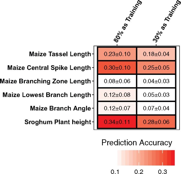
Performance of genomic prediction of trait measurement errors for five maize tassel traits plus sorghum plant height using 80% or 30% of genotypes as training sets. The text in each box represents the average prediction accuracy ± one standard error. Prediction accuracy is the correlations (r) between predicted trait measurement errors using gBLUP.

Discussion

Photographic systems are known for their relative simplicity, consistent data quality, flexibility, and cost–effectiveness. Thus, they have been widely used for high-throughput phenotyping. Because an image is a projection of a 3D structure onto a 2D plane, the sizes and shapes of different projections of the same 3D structure vary. This is one of the factors that can contribute to reduced phenotyping accuracy. In addition, precise object identification is crucial for the accurate measurement of many traits, such as length, but this task can be challenging using 2D images due to occlusion by nontarget structures (Gage et al., 2017; Zhou et al., 2019). Therefore, the conclusions of this study could apply to many high-throughput phenotyping pipelines that rely on 2D images.

In image-based phenotyping pipelines, errors can be introduced by imaging systems and/or trait extraction algorithms. Minimizing errors requires that the trait of interest be fully projected in the image. The traits examined in this study are unidimensional measurements of clearly defined morphological features. Consequently, for traits such as central spike length, phenotyping accuracy depends on the angle from which the image is shot and any occlusion of the highest branch point by other parts of the tassel. For manual measurements, these challenges can be easily overcome by simply rotating the tassels to find a clear measuring path. Similarly, the accuracy of image-based phenotyping can be improved by imaging traits from multiple angles and using mean measurements. Thus, in general, manual measurements more accurately reflect true trait values than automatically extracted trait values. However, for traits such as disease resistance, manual measurements are subject to additional sources of variability, such as rater effects and variation in lighting. Consequently, for traits of this type, the accuracies of data from automated phenotyping methods may actually be higher than those measured manually (Ghosal et al., 2018; Dobbels and Lorenz, 2019).

Because tassel architecture varies greatly in maize (Brown et al., 2011), different levels of tassel branch occlusion are expected. For populations that contain both “open” and “closed” tassel architecture, systematic inaccuracies in trait measurements would be expected to be confounded with tassel architecture. For example, extracting central spike length from an image with an occluded topmost branch point is more challenging than from an image with a nonoccluded central spike. Thus, trait values extracted from tassels with “closed” (dense) structures exhibit lower accuracy and more variability than those extracted from “open” tassels. Consequently, phenotypic measurement errors between ground truth and automatically extracted trait measurements, which are often assumed to be random, are instead partially regulated genetically.

Our GWAS of “open” and “closed” tassel structures identified two candidate genes known to contribute to tassel architecture, bif1 and ra3. Based on the reported mutant phenotypes, our two candidate genes for tassel openness participate in branch development but not in the elongation of inflorescence meristems, which may influence tassel length and central spike length (Bortiri and Hake, 2007; Tanaka et al., 2013; Zhang and Yuan, 2014). This implies that the results of our analyses of trait measurement errors of tassel length and central spike length, in which “open” and “closed” tassels exhibited significant differences in the means of trait measurement errors, are unlikely due to real pleiotropic effects of the genes that regulate openness. Furthermore, GWAS for trait measurement errors of central spike length found a candidate gene, lg1, that regulates tassel branch angle, a trait that in our dataset is not correlated with ground truth measurements of central spike length (Figures 5 and 7). Our finding that lg1 does not affect central spike length is consistent with our hypothesis that lg1 alters the accuracy of measurements of central spike length by altering branch angles. These results demonstrate that genetic factors, which we term GDMB, that do not regulate the traits of interest per se can still affect the accuracy of automatically extracted trait measurements and thus cannot be treated simply as different representations of the same underlying trait.

If trait measurement errors were largely random, then their effects could be mitigated by appropriate modeling, and substantial overlap would be expected between the GWAS results for ground truth and automatically extracted trait measurements. Yet, despite the high correlation (r² = 0.96) between BLUPs for ground truth and automatically extracted trait measurements of sorghum plant height in the data set of Salas Fernandez et al. (2017), the TASs identified via GWAS for these two traits exhibited only modest (∼40%) overlap. The GWAS for automatically extracted trait measurements detected two (Dw1 and Dw3) out of three height loci that were identified via the GWAS for ground truth with only slightly decreased estimated effects. This indicates that our inability to detect the third height locus (Dw2) in the GWAS for automatically extracted trait measurements was not the result of reduced power due to random errors within the BLUPs. The two TASs that GWAS for ground truth identified have both been previously reported as the most significant associations in their regions (Zhao et al., 2016; Salas Fernandez et al., 2017), making them unlikely to be false positives. Instead, the estimated effect size at Dw2 was greatly reduced (50%) compared to the Dw1 and Dw3 loci. Furthermore, the Dw2 region was associated with trait measurement errors (Figure 10;Supplemental Figure S4). This may explain our inability to detect this locus via GWAS of automatically extracted trait measurements.

Interestingly, our sorghum GWAS detected a significant association between trait measurement errors and the Dw3 locus, which has also been associated with leaf angle (Hart et al., 2001; Truong et al., 2015; Zhao et al., 2016; Mantilla-Perez and Salas Fernandez, 2017). Natural variation at this locus could lead to the presence of some genotypes with acute flag leaf angles, which could cause the algorithm to confuse flag leaves with panicle tips, thereby introducing noise into plant height estimates. This may explain the association between trait measurement errors and the Dw3 region. These results provide further support for the existence of GDMB and support the generalizability of their impacts to other image-based high-throughput phenotyping platforms.

The ability to phenotype larger populations is one of the advantages of high-throughput phenotyping protocols, and these larger population sizes are often assumed to offset the typically lower accuracies and precisions of such protocols compared to lower throughput manual measurements (Gage et al., 2018a; Ramstein et al., 2019). This assumption is valid to the extent that trait measurement errors are random (Figure 12A). Suppose that the investigator calculates genetic BLUPs for the trait of interest using the standard mixed linear model:

$$\mathit{y}=\mathit{X}\mathit{\beta }+\mathit{Zu}+\mathit{e}$$

where y is the n × 1 vector of observed phenotypes, $\mathit{\beta }$ is the p × 1 vector of fixed effects with design matrix $\mathit{X}$, $\mathit{u}\sim N\left(0,\mathit{G}{\sigma }_u^2\right)$ is the n × 1 vector of random genetic effects with design matrix Z and variance–covariance matrix $\mathit{G}$, and $\mathit{e}\sim N\left(0,\mathit{I}{\sigma }_e^2\right)$ is the n × 1 vector of residuals. Under the prevailing assumptions in the literature, the ground truth measurement of a phenotype (${\mathit{y}}_{gt}$) and its automatically extracted trait measurement (${\mathit{y}}_{\mathrm{auto}}$) have the same causal loci but different residual variances (Gage et al., 2018a), and these two phenotypes can be expressed as:

$${\mathit{y}}_{\mathrm{gt}}=\mathit{X}\mathit{\beta }+\mathit{Zu}+{\mathit{e}}_{\mathrm{gt}}$$

$${\mathit{y}}_{\mathrm{auto}}=\mathit{X}\mathit{\beta }+\mathit{Zu}+{\mathit{e}}_{\mathrm{auto}}$$

where ${\sigma }_{e_{\mathrm{gt}}}^2\ne {\sigma }_{e_{\mathrm{auto}}}^2$, and we have assumed that all other effects in both equations are equal by assumption. In some cases, systematic biases in ${\mathit{y}}_{\mathrm{auto}}$ may cause $\mathit{\beta }$ to differ between ${\mathit{y}}_{gt}$ and ${\mathit{y}}_{\mathrm{auto}}$, but this does not affect our conclusions. Then the differences between the ground truth and automatically extracted trait measurements can be defined as:

$$\begin{array}{c}\mathit{d}={\mathit{y}}_{\text{auto}}-{\mathit{y}}_{\text{gt}}\hfill \\ =\left(\mathit{X\beta }+\mathit{Zu}+{\mathit{e}}_{\text{auto}}\right)-\left(\mathit{X\beta }+\mathit{Zu}+{\mathit{e}}_{\text{gt}}\right)\hfill \\ \begin{array}{c}={\mathit{e}}_{\text{auto}}-{\mathit{e}}_{\text{gt}}\hspace{0.17em}\hspace{0.17em}\hspace{0.17em}\hspace{0.17em}\hspace{0.17em}\hspace{0.17em}\hspace{0.17em}\hspace{0.17em}\hspace{0.17em}\hspace{0.17em}\hspace{0.17em}\hspace{0.17em}\hspace{0.17em}\hspace{0.17em}\hspace{0.17em}\hspace{0.17em}\hspace{0.17em}\hspace{0.17em}\hspace{0.17em}\hspace{0.17em}\hspace{0.17em}\hspace{0.17em}\hspace{0.17em}\hspace{0.17em}\hspace{0.17em}\hspace{0.17em}\hspace{0.17em}\hspace{0.17em}\hspace{0.17em}\hspace{0.17em}\hspace{0.17em}\hspace{0.17em}\hspace{0.17em}\hspace{0.17em}\hspace{0.17em}\hspace{0.17em}\hspace{0.17em}\hspace{0.17em}\hspace{0.17em}\hspace{0.17em}\hspace{0.17em}\hspace{0.17em}\hspace{0.17em}\hspace{0.17em}\hspace{0.17em}\hspace{0.17em}\hspace{0.17em}\hspace{0.17em}\hspace{0.17em}\hspace{0.17em}\hspace{0.17em}\hspace{0.17em}\hspace{0.17em}\hspace{0.17em}\hspace{0.17em}\hspace{0.17em}\hspace{0.17em}\hspace{0.17em}\hspace{0.17em}\hspace{0.17em}\hspace{0.17em}\hspace{0.17em}\left(1\right)\end{array}\hfill \end{array}$$

Figure 12.

Theoretical explanation for the effects of genetically determined measurement biases on the accuracy of high-throughput phenotyping. A, General hypothesis assumes the trait measurement errors to be random. If this hypothesis stands, ground truth and auto-extracted trait measurements could be considered as two traits with the same causal loci (G is the same) but different heritabilities (i.e. Error and Error’ are not equal). However, our results show that the causal loci for auto-extracted trait measurements (G′) can be different from those for ground truth. This is due to the existence of genetic effects in error (G_error) for trait measurement errors. B, Increasing the population size and number of measurement replicates controls random errors by decreasing the proportion of random error in phenotype variation. However, this approach will be less likely to reduce the variance of genetic error. Instead, by reducing the variance of random error, the proportion of genetic error could increase together with genetic variance in proportion to the reduction of random error.

Thus, we expect no genetic associations with the differences between phenotyping methods.

However, our results demonstrate, as hypothesized by Liang et al. (2018) for maize biomass, that measurement errors for multiple traits in maize and sorghum can be influenced by genotype (Figures 7 and 10). As shown in Figure 6, a positive correlation was observed between the difference of ground truth and automatically extracted trait measurements of central spike length and the ground truth measurement of branch angle. Because no significant correlation was observed between the ground truth measurement of central spike length and branch angle, this suggests the presence of nonrandom components of trait measurement errors in our automated measurement of central spike length potentially introduced via the interaction between a tassel’s branch angle and the 2D imaging process. Let ${\mathit{y}}_{\mathrm{cs}}$ be the vector of ground truth measurements of central spike length and ${\mathit{y}}_{\mathrm{ba}}$ the vector of ground truth measurements of branch angle modeled as above using the standard mixed linear model:

$${\mathit{y}}_{\mathrm{cs}}=\mathit{X}{\mathit{\beta }}_{\mathrm{cs}}+\mathit{Z}{\mathit{u}}_{\mathrm{cs}}+{\mathit{e}}_{\mathrm{cs}}$$

$${\mathit{y}}_{\mathrm{ba}}=\mathit{X}{\mathit{\beta }}_{\mathrm{ba}}+\mathit{Z}{\mathit{u}}_{\mathrm{ba}}+{\mathit{e}}_{\mathrm{ba}}$$

Now let ${\mathit{y}}_{\mathrm{cs}}^{\text{'}}$ be the vector of automatically extracted measurements of central spike length. Following the assumptions discussed above, ${\mathit{y}}_{\mathrm{cs}}^{\text{'}}$ can be modeled identically to ${\mathit{y}}_{\mathrm{cs}}$. However, we now introduce the effect of a tassel’s branch angle on ${\mathit{y}}_{\mathrm{cs}}^{\text{'}}$ via the rate of change in central spike length with respect to branch angle, ${\mathrm{\lambda }}_{\mathrm{cs}:\mathrm{ba}}$, in a recursive linear system (Gianola and Sorensen, 2004; Eqs 13 and 14):

$$\begin{array}{c}{\mathit{y}}_{\text{cs}}^{\prime }={\lambda }_{\text{cs:ba}}{\mathit{y}}_{\text{ba}}+\mathit{X}{\mathit{\beta }}_{\text{cs}}+\mathit{Z}{\mathit{u}}_{\text{cs}}+{\mathit{e}}_{\text{cs}}^{\prime }\hfill \\ =\mathit{X}\left({\lambda }_{\text{cs:ba}}{\mathit{\beta }}_{\text{ba}}+{\mathit{\beta }}_{\text{cs}}\right)+\mathit{Z}\left({\lambda }_{\text{cs:ba}}{\mathit{u}}_{\text{ba}}+{\mathit{u}}_{\text{cs}}\right)+\left({\lambda }_{\text{cs:ba}}{\mathit{e}}_{\text{ba}}+{\mathit{e}}_{\text{cs}}^{\prime }\right)\hfill \\ \begin{array}{c}=X{\mathit{\beta }}^{*}+Z{\mathit{u}}^{*}+{\mathit{e}}^{*}\hspace{0.17em}\hspace{0.17em}\hspace{0.17em}\hspace{0.17em}\hspace{0.17em}\hspace{0.17em}\hspace{0.17em}\hspace{0.17em}\hspace{0.17em}\hspace{0.17em}\hspace{0.17em}\hspace{0.17em}\hspace{0.17em}\hspace{0.17em}\hspace{0.17em}\hspace{0.17em}\hspace{0.17em}\hspace{0.17em}\hspace{0.17em}\hspace{0.17em}\hspace{0.17em}\hspace{0.17em}\hspace{0.17em}\hspace{0.17em}\hspace{0.17em}\hspace{0.17em}\hspace{0.17em}\hspace{0.17em}\hspace{0.17em}\hspace{0.17em}\hspace{0.17em}\hspace{0.17em}\hspace{0.17em}\hspace{0.17em}\hspace{0.17em}\hspace{0.17em}\hspace{0.17em}\hspace{0.17em}\hspace{0.17em}\hspace{0.17em}\hspace{0.17em}\hspace{0.17em}\hspace{0.17em}\hspace{0.17em}\hspace{0.17em}\hspace{0.17em}\hspace{0.17em}\hspace{0.17em}\hspace{0.17em}\hspace{0.17em}\hspace{0.17em}\hspace{0.17em}\hspace{0.17em}\hspace{0.17em}\hspace{0.17em}\hspace{0.17em}\hspace{0.17em}\hspace{0.17em}\hspace{0.17em}\hspace{0.17em}\hspace{0.17em}\hspace{0.17em}\left(2\right)\end{array}\hfill \end{array}$$

where ${\mathit{\beta }}^{\mathit{*}}={\lambda }_{\mathrm{cs}:\mathrm{ba}}{\mathit{\beta }}_{\mathrm{ba}}+{\mathit{\beta }}_{\mathrm{cs}}$, ${\mathit{u}}^{\mathit{*}}={\lambda }_{\mathrm{cs}:\mathrm{ba}}{\mathit{u}}_{\mathrm{ba}}+{\mathit{u}}_{\mathrm{cs}}$, and ${\mathit{e}}^{*}={\lambda }_{\mathrm{cs}:\mathrm{ba}}{\mathit{e}}_{\mathrm{ba}}+{\mathit{e}}_{\mathrm{cs}}^{\prime }$. Equation 2 has the form of the standard mixed linear model; however, a naïve analysis that does not account for the bias introduced by the interaction between branch angle and the 2D imaging procedure will estimate ${\mathit{u}}^{*}$, which is not an unbiased estimate of ${\mathit{u}}_{\mathrm{cs}}$.

We can now re-express $\mathit{d}$ as

$$\begin{array}{c}\mathit{d}={\mathit{y}}_{\text{cs}}^{\prime }-{\mathit{y}}_{\text{cs}}\hfill \\ =({\lambda }_{\text{cs:ba}}{\mathit{y}}_{\text{ba}}+\mathit{X}{\mathit{\beta }}_{\text{cs}}+\mathit{Z}{\mathit{u}}_{\text{cs}}+{\mathit{e}}_{\text{cs}}^{\prime })-\left(\mathit{X}{\mathit{\beta }}_{\text{cs}}+\mathit{Z}{\mathit{u}}_{\text{cs}}+{\mathit{e}}_{\text{cs}}\right)\hfill \\ \begin{array}{c}={\lambda }_{\text{cs:ba}}\left(\mathit{X}{\mathit{\beta }}_{\text{ba}}+\mathit{Z}{\mathit{u}}_{\text{ba}}+{\mathit{e}}_{\text{ba}}\right)+\left({\mathit{e}}_{\text{cs}}^{\prime }-{\mathit{e}}_{\text{cs}}\right)\hspace{0.17em}\hspace{0.17em}\hspace{0.17em}\hspace{0.17em}\hspace{0.17em}\hspace{0.17em}\hspace{0.17em}\hspace{0.17em}\hspace{0.17em}\hspace{0.17em}\hspace{0.17em}\hspace{0.17em}\hspace{0.17em}\hspace{0.17em}\hspace{0.17em}\hspace{0.17em}\hspace{0.17em}\hspace{0.17em}\hspace{0.17em}\hspace{0.17em}\hspace{0.17em}\hspace{0.17em}\hspace{0.17em}\hspace{0.17em}\hspace{0.17em}\hspace{0.17em}\hspace{0.17em}\hspace{0.17em}\hspace{0.17em}\hspace{0.17em}\hspace{0.17em}\hspace{0.17em}\hspace{0.17em}\hspace{0.17em}\hspace{0.17em}\hspace{0.17em}\hspace{0.17em}\hspace{0.17em}\hspace{0.17em}\hspace{0.17em}\hspace{0.17em}\hspace{0.17em}\hspace{0.17em}\hspace{0.17em}\hspace{0.17em}\hspace{0.17em}\hspace{0.17em}\hspace{0.17em}\hspace{0.17em}\left(3\right)\end{array}\hfill \end{array}$$

The trait measurement errors now include the term ${\lambda }_{\mathrm{cs}:\mathrm{ba}}\mathit{Z}{\mathit{u}}_{\mathrm{ba}}$, which we have termed GDMB, that is introduced as the result of interactions between the phenotyping method and a nontarget phenotype. The presence of GDMB can affect both the magnitude and sign of $\mathit{d}$, which is supported by our observations in Figures 4 and 5. This also accounts for our identification of a candidate gene for branch angle in the GWAS for the difference between ground truth and automated measurements of central spike length (Figure 7).

The recursive model also helps explain the smaller number of TASs observed in the GWAS for auto-extracted trait measurements using central spike length relative to that of ground truth measurements of central spike length. As shown by Equation 2, the use of genetic BLUPs from fitting a standard mixed linear model to automatically extracted trait measurements conflates the genetic contributions of two traits. Thus, the estimated effects of TASs identified via GWAS conducted using such BLUPs are similarly conflated. Because multiple genetic sources co-exist in trait measurement errors, the complicated interactions among these genetic sources with ground truth (as shown in Figure 6) can result in over or underestimation of allelic effects or even sign changes. This may explain the poor overlap among the TASs identified via GWAS using automatically extracted trait measurements and ground truth for all five tassel traits in spite of their moderate-to-high phenotypic correlations.

Furthermore, assuming that genetic effects and residuals are independent, the variance of the automated measurement of the phenotype given by Equation 2 is:

$$\begin{array}{c}\text{Var}\left({\mathit{y}}_{\text{cs}}^{\prime }\right)=\text{Var}\left({\lambda }_{\text{cs:ba}}{\mathit{u}}_{\text{ba}}+{\mathit{u}}_{\text{cs}}\right)+\text{Var}\left({\lambda }_{\text{cs:ba}}{\mathit{e}}_{\text{ba}}+{\mathit{e}}_{\text{cs}}^{\prime }\right)\hfill \\ =\left({\lambda }_{\text{cs:ba}}^2{\sigma }_{{\mathrm{u}}_{\text{ba}}}^2+{\sigma }_{u_{\text{cs}}}^2+2{\lambda }_{\text{cs:ba}}{\sigma }_{u_{\text{ba}}{u}_{\text{cs}}}\right)+\left({\lambda }_{\text{cs:ba}}^2{\sigma }_{e_{\text{ba}}}^2+{\sigma }_{e_{\text{'}\text{cs}}}^2+2{\lambda }_{\text{cs:ba}}{\sigma }_{e_{\text{ba}}{e}^{\prime }{}_{\text{cs}}}\right)\hfill \\ \begin{array}{c}=\left({\sigma }_{u_{\text{cs}}}^2+{\sigma }_{e^{\prime }{}_{\text{cs}}}^2\right)+{\lambda }_{\text{cs:ba}}^2\left({\sigma }_{u_{\text{ba}}}^2+{\sigma }_{e_{\text{ba}}}^2\right)+2{\lambda }_{\text{cs:ba}}\left({\sigma }_{u_{\text{ba}}{u}_{\text{cs}}}+{\sigma }_{e_{\text{ba}}{e}^{\prime }{}_{\text{cs}}}\right)\hspace{0.17em}\hspace{0.17em}\left(4\right)\end{array}\hfill \end{array}$$

In contrast, the variance of the ground truth measurements for central spike length (${\mathit{y}}_{\mathrm{cs}}$) corresponds to the leftmost term in parentheses on the final line. This equation shows that the variance of the auto-extracted trait measurements includes the genetic and residual variances of branch angle along with their respective covariances with central spike length. Inclusion of these components can increase or reduce the variance of the automatically extracted trait measurements, depending on the signs and magnitudes of the covariance term in Equation 4 relative to the combined magnitudes of the variances. Changes in the power to detect a significant association at any given marker then depend on the heritabilities of each trait, their co-heritability, and the combined effects of the marker for each trait. If the signs of the marker effects on each trait are equal, the combined effect will be greater in magnitude, increasing the power to detect an association. However, if the signs are opposite, reduced power can result from a reduction in the magnitude of the combined effect toward zero, or incorrect inference on the effect direction can result when the sign of the combined effect is reversed with respect to the sign of the effect on the focal trait. Furthermore, false positives can be introduced when a marker truly has no effect on the focal trait but has a nonzero effect on the nonfocal trait. The net result of these changes would be to complicate the interpretation of the GWAS results.

Increasing population size to reduce the effects of random errors and to increase allelic replication is a popular strategy for improving the power of GWAS. However, Equation 4 shows that the additional variance components introduced by automated phenotyping are modulated by $\lambda$, which will have a lower bound defined by the phenotyping method and biological pleiotropy between the target trait and other confounding traits (Figure 12B). Therefore, larger population sizes cannot be simply substituted for an understanding of the relationships among multiple traits and their interactions with the phenotyping method. In fact, it is possible that weakly associated effects introduced by GDMB will reach statistical significance as a consequence of the increased statistical power achieved by using larger populations, which could complicate the interpretation of results (Figure 12B). Moreover, feature extraction pipelines are commonly developed using only modest numbers of genotypes. Our results suggest that such strategies might not be sufficient when testing large and diverse populations because the use of a small number of genotypes for pipeline development could result in systematic, genetic bias due to a lack of phenotypic and/or genetic representation. This is especially important for pipelines using machine learning, which can generate biased results when the training dataset is insufficiently representative of the full population (Mehrabi et al., 2019).

Our study also showed that trait measurement errors for multiple traits were correlated with multiple ground truth measurement of other traits, which could contribute to the observed differences in error means and variances between the two tassel structures (Figure 4). This indicates that trait measurement errors can exhibit complex dependencies on multiple genetic sources that have thus far been assumed to be absent. The model presented in Equation 2 could easily be extended to account for more complex dependencies, including possible genetic effects on the residual variances.

Both maize and sorghum have been reported to exhibit extensive population structure (Liu et al., 2003; Morris et al., 2013), which could affect the GDMB that we observed if tassel morphology or height is associated with population structure. If population structure is included in the GWAS model, the effects of SNPs associated with population structure on GDMB would be controlled. Evaluating such a scenario should be the subject of future work.

However, GDMB may also provide an opportunity to better understand the genetic basis of complex traits. In this study, GWAS on trait measurement errors in two species identified loci that potentially contribute to plant architecture (Figures 7B and 9C). Considering that many traits, such as plant height and yield, are composite and can be partitioned into multiple components for genetic analyses (Otegui and Bonhomme, 1998; Brown et al., 2008; Peng et al., 2011; Li et al., 2015), it would be interesting to explore the possibility of using the difference between two trait measurements (e.g. two different automated phenotyping pipelines) as an additional approach to identify additional causal loci that contribute to phenotypic variation.

In other cases, GDMB may simply represent an undesirable source of both noise and potential false positive TASs. In these cases, GDMB can instead be predicted and controlled. As shown in Figure 11, incorporating genomic information makes it possible to construct models using both ground truth and automatically extracted trait measurements for a subset of the population to predict the direction and magnitude of GDMB across a larger population. For traits in which GDMB comprised a substantial fraction of measurement error, such as maize tassel length and sorghum plant height, data from even a relatively small subset of the population (e.g. 30% of individuals) was sufficient to achieve prediction accuracy close to that achieved with data from 80% of the population. It may therefore be possible to estimate and correct for GDMB via genomic prediction, achieving more accurate estimates of trait values for downstream quantitative genetic or breeding applications. We used predicted GDMB to re-calibrate automated measurements, but GWAS results were inconsistent among maize tassel and sorghum height traits, perhaps due to the small size of the training sets (N = 100) used for prediction.

The strong correlations between morphological traits and measurement errors also suggests that it may be possible to control the effects of GDMB by considering the causal relationships among phenotypes in GWAS through multi-trait GWAS or structural equation modeling GWAS (Turley et al., 2018; Momen et al., 2019), which is the natural extension of Equation 2. Furthermore, our study also suggests that incorporating information from other morphological traits—possibly with the use of machine learning to recalibrate the trait measurements—is an alternative worthy of study.

Materials and methods

Plant materials and tassel imaging

The SAM Z. mays diversity panel was grown during the summer 2017 at the Iowa State University, Ag Engineering and Agronomy Research Farm in Boone, IA. One tassel from each of 339 genotypes was collected on the first day of anthesis and imaged indoors (Figure 1A). Tassels were mounted upright on a remote-controlled base that was programmed to rotate clockwise in steps of 90°. All tassels were attached to the holder such that the lowest branch was to the right in the camera’s viewfinder and avoided occlusion by other branches as much as possible to ensure that the lowest branch and the main axis were fully within the image and in the same plane (Figure 1B; view 1). A yellow scale with a length of 1 inch (2.54 cm) was placed next to the holder to serve as the unit reference for later data conversion. Images were captured using a Canon EOS 5DSR camera with a Canon EF100 mm f/2.8 L Macro IS USM lens. The camera was set up 2.5 m from the tassel and mounted at a height of 122 cm. After the first image was taken, the holder and tassel were rotated 90° clockwise before shooting the second image (Figure 1B; view 2). This process was repeated two times until the tassel had been rotated 270° from its original position (Figure 1B; views 3 and 4). The tassel was then rotated so that the lowest branch pointed to the left in the camera’s viewfinder and the angle between the second lowest branch and the main axis was as clearly visible as possible before shooting the fifth image (Figure 1B; view 5). Hence, each tassel was imaged five times.

Trait extraction

Our TI-TET pipeline requires the identification of the bottom end of the main rachis located below the lowest branch point for building the tassel’s skeleton (Supplemental Protocol). In some cases, a bent tassel was encountered, thus making it difficult to keep the tassel upright in the stand, which could complicate the automated detection of the bottom end. To cope with such problems, we manually marked the bottom end of the tassel in each image using a custom-built MATLAB application by drawing a red rectangle to recognize the starting point for the skeleton built algorithm to begin with. These annotated images were then used for tassel segmentation and trait extraction.

Automated trait extraction involved the following steps: (1) tassel segmentation; (2) measurement of traits from the segmented tassel; and (3) conversion of trait values from pixels to metric units using the segmented reference scale (Figure 1C; Supplemental Protocol). Trait measurements were performed in a fully automated manner (described in the Supplemental Protocol).

A total of five tassel traits were extracted from the images, including tassel length, central spike length, branching zone length, lowest branch length, and lowest branch angle (Supplemental Data Set S5). Tassel length was defined as the length of the main tassel axis from the lowest branch point to the tip of the central spike. The central spike length was measured from the top-most branch point to the tip of the central spike. The branching zone length, which is the length of the main axis between the lowest branch point and the top-most branch point, was calculated as the difference between tassel length and central spike length. The lowest branch length and branch angle were defined as the length from the lowest branch point to the tip of the lowest branch and the angle between the lowest branch and the main axis in the image (Figure 1C). The pixel-to-cm conversion was achieved by measuring the pixel length of the 1 inch (2.54 cm) yellow scale in each image to obtain an image-specific ratio of pixels to cm. These five tassel traits were also manually collected from the same tassels once the photos were taken using a ruler for length traits and a protractor for the lowest branch angle. All ground truth measurements were collected by a single person indoors under controlled lighting conditions.

Phenotyping tassel structure

An additional two replicates of the SAM panel were grown during the summer 2017 at Iowa State University’s Curtiss Farm, Ames, IA (10 km east of the ISU Ag Engineering and Agronomy Research Farm). Each genotype was planted in one row containing 12 plants with roughly 15 cm (6 inches) between plants and 89 cm (35 inches) between rows. Due to poor germination and storm damage, tassels of only 335 genotypes were intact on the first day of anthesis for each genotype and manually characterized as “open” or “closed” based on whether the top-most branch points of each genotype’s tassels could be seen without close inspection (Figure 3). If the base of the central spike was not occluded by other branches from the same tassel, it was considered to be “open”, while tassels with an occluded central spike base were considered to be “closed”. Genotypes classified as “open” in one replicate and “closed” in the other were classified as “partially open”.

Correlations among trait measurement errors and tassel traits

Pearson correlation coefficients among trait measurement errors of five tassel traits and their ground truth in addition to branch number were computed using the “cor ()” function of R. To further investigate the influence of tassel architecture traits on the variance of phenotypic measurement errors, we then built multiple regression models for phenotypic measurement errors using ground truth measurements and tassel openness as predictors. Models were selected using backward elimination and the Akaike information criterion (AIC), with the full model containing all six manual measured tassel traits and openness.

GWAS on tassel traits and tassel structure

GWAS was conducted using the SNP dataset described by Leiboff et al. (2015) in R (version 3.4.2) and FarmCPUpp (Liu et al., 2016; Kusmec and Schnable, 2018). Principal component analysis was conducted on the SNP data using the ‘prcomp’ function of R. Model selection was performed and optimized using AIC. The first three PCs, which explained 3.4%, 2.4%, and 1.6% of the variance, respectively, were then used as covariates to control for population structure. FarmCPUpp’s optimum bin selection procedure was used with bin sizes of 10 kb, 50 kb, and 100 kb. P-values for each SNP were transformed using the “qvalue” package (Storey et al., 2020) to estimate the local false discovery rate (Efron et al., 2001; Efron, 2007). SNPs with q-values <0.05 were declared to be statistically significant.

For tassel structure, “closed,” “partially open,” and “open” tassels were numerically coded as 0, 0.5, and 1, respectively. Automated and ground truth measurements of tassel traits, along with each trait’s measurement error (automatically extracted trait measurements—ground truth), were used as phenotypes for GWAS.

Candidate gene screening for GWAS results

TASs were compared to a list of 69 known maize inflorescence genes (Supplemental Data Set S3) based on a review of the literature. Because the length of LD blocks varies along chromosomes, genes from this list were considered to be candidate genes if their physical positions were within a 120-kb window centered on a TAS (i.e. 60-kb upstream and 60-kb downstream). For every GWAS that identified genes from this list, a permutation test with 1,000 iterations was performed by randomly drawing the same number of TASs from the genome-wide SNPs, controlling for proximity to the nearest gene and the minor allele frequency (MAF) distribution. Proximity to the nearest gene was defined as “within gene”, “$\le$5kb to the nearest gene”, and “>5kb to the nearest gene”. MAF was assigned to one of four categories: (0, 0.05], (0.05, 0.20], (0.20, 0.35], and (0.35, 0.5]. The sampled SNPs were then screened for candidate genes using the same procedure.

Genotyping lg1 mutants

When necessary, lg1-mu/lg1-mu and lg1-mu/Lg1 genotypes were distinguished using primers listed in Supplemental Table S3.

Genomic prediction for trait measurement errors and genetic analysis using sorghum plant height data

Two sorghum plant height datasets for 301 genotypes from the SAP were used in this study (Salas Fernandez et al. 2017). These data sets contain User-interactive Individual Plant Height Extraction (UsIn-PHe) based on dense stereo 3D reconstruction and Automatic Hedge-based Plant Height Extraction (Auto-PHe) based on dense stereo 3D reconstruction measurements of plant height. The semi-automated UsIn-PHe were used as the ground truth due to its high accuracy (r²=0.994). BLUP of genetic effects for plant height was performed using the lme4 package (Bates et al., 2014) in R using the following model: lmer(phenotype ∼ (1| genotype) + (1| location) + (1| genotype: location) + (1| location: replicates)). Trait measurement errorsTrait measurement errors were calculated as the difference between BLUPs of Auto-PHe and UsIn-PHe (Supplemental Data Set S5). Variance component decomposition for trait measurement errors was performed using ridge regression BLUP version 4.2 (Endelman, 2011, http://cran.r-project.org/web/packages/rrBLUP/). Two models were tested: (1) gBLUP using the additive genetic relationship matrix and (2) RKHS regression using the Gaussian kernel and the Euclidean distance estimated from SNPs to consider possible nonadditive genetic effects.

GWAS on BLUPs of UsIn-PHe, Auto-PHe, and their differences was conducted using the 146,865 SNPs and methods described in Zhou et al. (2019). Significantly associated SNPs were determined as in the GWAS for tassel traits. We scanned for TASs that were close to of the four known segregating plant height loci in this panel: Dw1, Dw2, Dw3, and qHT7.1 (Brown et al., 2008; Thurber et al., 2013; Morris et al., 2013; Li et al., 2015; Zhao et al., 2016).

Evaluation of the predictability of measurement errors

Genomic predictions of the five tassel traits and sorghum height were performed using gBLUP as described above. Two approaches, one using 80% and the other using 30% of genotypes randomly sampled from the full population without duplication, were chosen as training set and the remaining 20% and 70% of genotypes from the population, respectively, served as the test set. For each trait, this process was repeated for 100 iterations. For each iteration, the correlation between predicted trait measurement errors and true errors was computed using the “cor()” function in R. The averaged correlations of the 100 iterations were then used to estimate the prediction accuracy.

Accession numbers

Sequence data from this article can be found in the GenBank/EMBL libraries under the accession numbers listed in Supplemental Data Set S3.

The phenotype data used in this study are provided in Supplemental Data Set S5. The codes used for automated tassel segmentation, skeleton construction and trait extraction are available at https://github.com/schnablelab/Tassel-Image-Trait-Extraction-Tool.

Supplemental data

The following materials are available in the online version of this article.

Supplemental Figure S1. Phenotyping accuracy varies among tassel openness classes of the full population.

Supplemental Figure S2. Box and violin plots of absolute trait measurement errors (difference between automated and ground truth measurements) measured as deviation from ground truth and its value in ratio to ground truth stratified by tassel openness.

Supplemental Figure S3. Pearson correlation coefficients between ground truth (.GT) and absolute values of trait measurement errors (.error).

Supplemental Figure S4. Manhattan and QQ plots for 19 traits plotted by −log₁₀(P-value).

Supplemental Figure S5. Effect of the ra3 mutation on tassel branching architecture.

Supplemental Figure S6. Phenotypic correlations and estimated genetic components in variance of trait measurement errors.

Supplemental Figure S7. Manhattan plots for GWAS on sorghum plant height using ground truth measurements, auto-extracted trait measurements (Auto), and trait measurement errors (Error).

Supplemental Figure S8. Box and violin plots of the estimated effects of 257 SNPs within 600 kb of Dw2 from GWAS sorghum plant height using ground truth measurements, auto-extracted trait measurements, and trait measurement errors.

Supplemental Table S1. Multiple regression models for trait measurement errors (.errors) using ground truth measurements (.GT) and tassel openness as predictors.

Supplemental Table S2. List of TASs in sorghum plant height GWAS for ground truth measurements (GT), auto-extracted trait measurements (Auto), and trait measurement errors (Error).

Supplemental Table S3. Primers used for genotyping the lg1-mu mutants.

Supplemental Protocol. TI-TET extendable phenotyping pipeline.

Supplemental Data Set S1. Summary of the test statistics for Student’s t test for data shown in the figures.

Supplemental Data Set S2. List of TASs in openness and five tassel traits GWAS for ground truth measurements (.GT), auto-extracted trait measurements (.Auto), and trait measurement errors (.Error).

Supplemental Data Set S3. Sixty-nine known maize tassel-related genes.

Supplemental Data Set S4. GWAS results for SNPs within 600 kb of Dw2 from GWAS on ground truth measurements (GT), auto-extracted trait measurements (Auto), and trait measurement errors (Error) of sorghum plant height.

Supplemental Data Set S5. List of phenotypic values of maize tassel traits and sorghum plant height used in GWAS.

 

P.S.S., S.S., and B.G. conceived the original research plan and supervised the experiments and data analyses; P.S.S., Y.Z., L.A., S.V.M., and S.S. designed the experiments; L.A., Y.Z., T.Z.J., and S.V.M. developed the phenotype extraction pipeline and conducted phenotype extractions; Y.Z. and A.K conducted most of the experiments and analyses; M.G.S.F. and J.C.S. assisted with the interpretation of results; P.S.S., L.A., M.G.S.F, J.C.S., S.V.M., A.K., and Y.Z. wrote the article with contributions from all the authors.

The author responsible for distribution of materials integral to the findings presented in this article in accordance with the policy described in the Instructions for Authors (https://academic.oup.com/plcell) is: Patrick S. Schnable (schnable@iastate.edu).

References

- AL-Tam F, Adam H, Anjos A, Lorieux M, Larmande P, Ghesquière A, Jouannic S, Shahbazkia H (2013) P-TRAP: a panicle trait phenotyping tool. BMC Plant Biol 13: 122. [DOI] [PMC free article] [PubMed] [Google Scholar]
- Anderson SL, Murray SC, Malambo L, Ratcliff C, Popescu S, Cope D, Chang A, Jung J, Thomasson JA (2019) Prediction of maize grain yield before maturity using improved temporal height estimates of unmanned aerial systems. Plant Phenome J 2: 1–15 [Google Scholar]
- Araus JL, Cairns JE (2014) Field high-throughput phenotyping: the new crop breeding frontier. Trends Plant Sci 19: 52–61 [DOI] [PubMed] [Google Scholar]
- Barazesh S, McSteen P (2008) Barren inflorescence1 functions in organogenesis during vegetative and inflorescence development in maize. Genetics 179: 389–401 [DOI] [PMC free article] [PubMed] [Google Scholar]
- Bates D, Mächler M, Bolker B, Walker S (2014) Fitting linear mixed-effects models using lme4. arXiv preprint arXiv: 1406.5823
- Bortiri E, Hake S (2007) Flowering and determinacy in maize. J Exp Bot 58: 909–916 [DOI] [PubMed] [Google Scholar]
- Brown PJ, Rooney WL, Franks C, Kresovich S (2008) Efficient mapping of plant height quantitative trait loci in a sorghum association population with introgressed dwarfing genes. Genetics 180: 629–637 [DOI] [PMC free article] [PubMed] [Google Scholar]
- Brown PJ, Upadyayula N, Mahone GS, Tian F, Bradbury PJ, Myles S, Holland JB, Flint-Garcia S, McMullen MD, Buckler ES, et al. (2011) Distinct genetic architectures for male and female inflorescence traits of maize. PLoS Genet 7: p.e1002383. [DOI] [PMC free article] [PubMed] [Google Scholar]
- Choudhury SD, Samal A, Awada T (2019) Leveraging image analysis for high-throughput plant phenotyping. Front Plant Sci 10: 508. [DOI] [PMC free article] [PubMed] [Google Scholar]
- Crowell S, Falcao AX, Shah A, Wilson Z, Greenberg AJ, McCouch SR (2014) High-resolution inflorescence phenotyping using a novel image-analysis pipeline, PANorama. Plant Physiol 165: 479–495 [DOI] [PMC free article] [PubMed] [Google Scholar]
- Dobbels AA, Lorenz AJ (2019) Soybean iron deficiency chlorosis high throughput phenotyping using an unmanned aircraft system. Plant Methods 15: 97. [DOI] [PMC free article] [PubMed] [Google Scholar]
- Duvick DN (2005) Genetic progress in yield of Untied States maize (Zea mays L.). Maydica 50: 193–202 [Google Scholar]
- Duvick DN, Cassman K (1999) Post-green revolution trends in yield potential of temperate maize in the United States. Crop Sci 39: 1622–1630 [Google Scholar]
- Efron B (2007) Size, power and false discovery rates. Ann Stat 35: 1351–1377 [Google Scholar]
- Efron B, Tibshirani R, Storey JD, Tusher V (2001) Empirical bayes analysis of a microarray experiment. J Am Stat Assoc 96: 1151–1160 [Google Scholar]
- Endelman JB (2011) Ridge regression and other kernels for genomic selection with R Package rrBLUP. Plant Genome 4: 250 [Google Scholar]
- Gage JL, de Leon N, Clayton MK (2018a) Comparing genome-wide association study results from different measurements of an underlying phenotype. Genes Genomes Genet 8: 3715–3722 [DOI] [PMC free article] [PubMed] [Google Scholar]
- Gage JL, Miller ND, Spalding EP, Kaeppler SM, de Leon N (2017) TIPS: a system for automated image-based phenotyping of maize tassels. Plant Methods 13: 21. [DOI] [PMC free article] [PubMed] [Google Scholar]
- Gage JL, White MR, Edwards J, Kaeppler S, de Leon N (2018b) Selection signatures underlying dramatic male inflorescence transformation during modern hybrid maize breeding. Genetics 210: 1125–1138 [DOI] [PMC free article] [PubMed] [Google Scholar]
- Gaillard M, Miao C, Schnable J, Benes B (2020) Voxel carving based 3D reconstruction of sorghum identifies genetic determinants of radiation interception efficiency. Plant Direct 4: e00255. [DOI] [PMC free article] [PubMed] [Google Scholar]
- Gallavotti A, Long JA, Stanfield S, Yang X, Jackson D, Vollbrecht E, Schmidt RJ (2010) The control of axillary meristem fate in the maize ramosa pathway. Development 137: 2849–2856 [DOI] [PMC free article] [PubMed] [Google Scholar]
- Galli M, Liu Q, Moss BL, Malcomber S, Li W, Gaines C, Federici S, Roshkovan J, Meeley R, Nemhauser JL, et al. (2015). Auxin signaling modules regulate maize inflorescence architecture. Proc Natl Acad Sci U S A 112: 13372–13377 [DOI] [PMC free article] [PubMed] [Google Scholar]
- Ghosal S, Blystone D, Singh AK, Ganapathysubramanian B, Singh A, Sarkar S (2018) An explainable deep machine vision framework for plant stress phenotyping. Proc Natl Acad Sci U S A 115: 4613–4618 [DOI] [PMC free article] [PubMed] [Google Scholar]
- Gianola D, Sorensen D (. 2004) Quantitative genetic models for describing simultaneous and recursive relationships between phenotypes. Genetics 167: 1407–1424 [DOI] [PMC free article] [PubMed] [Google Scholar]
- Hart GE, Schertz KF, Peng Y, Syed NH (2001) Genetic mapping of Sorghum bicolor (L.) Moench QTLs that control variation in tillering and other morphological characters. Theor Appl Genet 103: 1232–1242 [Google Scholar]
- He JQ, Harrison RJ, Li B (2017) A novel 3D imaging system for strawberry phenotyping. Plant Methods 13: 93. [DOI] [PMC free article] [PubMed] [Google Scholar]
- Holman FH, Riche AB, Michalski A, Castle M, Wooster MJ, Hawkesford MJ (2016) High throughput field phenotyping of wheat plant height and growth rate in field plot trials using UAV based remote sensing. Remote Sens 8: 1031 [Google Scholar]
- Kircher M, Kelso J (2010) High-throughput DNA sequencing - Concepts and limitations. BioEssays 32: 524–536. [DOI] [PubMed] [Google Scholar]
- Kusmec A, Schnable PS (2018) FarmCPUpp: efficient large-scale genomewide association studies. Plant Direct 2: e00053. [DOI] [PMC free article] [PubMed] [Google Scholar]
- Leiboff S, Li X, Hu H-C, Todt N, Yang J, Li X, Yu X, Muehlbauer GJ, Timmermans MCP, Yu J, et al. (2015). Genetic control of morphometric diversity in the maize shoot apical meristem. Nat Commun 6: 1–10 [DOI] [PMC free article] [PubMed] [Google Scholar]
- Lewis MW, Bolduc N, Hake K, Htike Y, Hay A, Candela H, Hake S (2014) Gene regulatory interactions at lateral organ boundaries in maize. Development 141: 4590–4597 [DOI] [PubMed] [Google Scholar]
- Li M, Shao MR, Zeng D, Ju T, Kellogg EA, Topp CN (2020) Comprehensive 3D phenotyping reveals continuous morphological variation across genetically diverse sorghum inflorescences. New Phytol 226: 1873–1885 [DOI] [PMC free article] [PubMed] [Google Scholar]
- Li X, Tesso TT, Yu J, Li X, Fridman E (2015) Dissecting repulsion linkage in the dwarfing gene Dw3 region for sorghum plant height provides insights into heterosis. Proc Natl Acad Sci U S A 112: 11823–11828 [DOI] [PMC free article] [PubMed] [Google Scholar]
- Liang Z, Pandey P, Stoerger V, Xu Y, Qiu Y, Ge Y, Schnable JC (2018) Conventional and hyperspectral time-series imaging of maize lines widely used in field trials. Gigascience 7: 1–11 [DOI] [PMC free article] [PubMed] [Google Scholar]
- Liu K, Goodman M, Muse S, Smith JS, Buckler E, Doebley J (2003) Genetic structure and diversity among maize inbred lines as inferred from DNA microsatellites. Genetics 165: 2117–2128 [DOI] [PMC free article] [PubMed] [Google Scholar]
- Liu X, Huang M, Fan B, Buckler ES, Zhang Z (2016) Iterative usage of fixed and random effect models for powerful and efficient genome-wide association studies. PLoS Genet 12: e1005767. [DOI] [PMC free article] [PubMed] [Google Scholar]
- Lobet G, Koevoets IT, Noll M, Meyer PE, Tocquin P, Pagès L, Périlleux C (2017) Using a structural root system model to evaluate and improve the accuracy of root image analysis pipelines. Front Plant Sci 8: 447. [DOI] [PMC free article] [PubMed] [Google Scholar]
- Mantilla-Perez MB, Salas Fernandez MG (2017) Differential manipulation of leaf angle throughout the canopy: Current status and prospects. J Exp Bot 68: 5699–5717 [DOI] [PubMed] [Google Scholar]
- McCormick RF, Truong SK, Mullet JE (2016) 3D sorghum reconstructions from depth images identify QTL regulating shoot architecture. Plant Physiol 172: 823–834 [DOI] [PMC free article] [PubMed] [Google Scholar]
- Mehrabi N, Morstatter F, Saxena N, Lerman K, Galstyan A (2019) A survey on bias and fairness in machine learning. arXiv preprint arXiv:1908.09635
- Momen M, Campbell MT, Walia H, Morota G (2019) Utilizing trait networks and structural equation models as tools to interpret multi-trait genome-wide association studies. Plant Methods 15: 1–14 [DOI] [PMC free article] [PubMed] [Google Scholar]
- Morris GP, Ramu P, Deshpande SP, Hash CT, Shah T, Upadhyaya HD, Riera-Lizarazu O, Brown PJ, Acharya CB, Mitchell SE, et al. (2013). Population genomic and genome-wide association studies of agroclimatic traits in sorghum. Proc Natl Acad Sci U S A 110: 453–458 [DOI] [PMC free article] [PubMed] [Google Scholar]
- Otegui ME, Bonhomme R (1998) Grain yield components in maize. Field Crop Res 56: 247–256 [Google Scholar]
- Peng B, Li YX, Wang Y, Liu C, Liu ZZ, Tan W, Zhang Y, Wang D, Shi Y, Sun B, et al. (2011) QTL analysis for yield components and kernel-related traits in maize across multi-environments. Theor Appl Genet 122: 1305–1320 [DOI] [PubMed] [Google Scholar]
- Ramstein GP, Jensen SE, Buckler ES (2019) Breaking the curse of dimensionality to identify causal variants in Breeding 4. Theor Appl Genet 132: 559–567 [DOI] [PMC free article] [PubMed] [Google Scholar]
- Salas Fernandez MG, Bao Y, Tang L, Schnable PS (2017) A high-throughput, field-based phenotyping technology for tall biomass crops. Plant Physiol 174: 2008–2022 [DOI] [PMC free article] [PubMed] [Google Scholar]
- Satoh-Nagasawa N, Nagasawa N, Malcomber S, Sakai H, Jackson D (2006) A trehalose metabolic enzyme controls inflorescence architecture in maize. Nature 441: 227–230 [DOI] [PubMed] [Google Scholar]
- Schuetz SH, Mock JJ (1978) Genetics of tassel branch number in maize and its implications for a selection program for small tassel size. Theor Appl Genet 53: 265–271 [DOI] [PubMed] [Google Scholar]
- Slatko BE, Gardner AF, Ausubel FM (2018) Overview of next-generation sequencing technologies. Curr Protoc Mol Biol 122: e59. [DOI] [PMC free article] [PubMed] [Google Scholar]
- Storey JD, Bass AJ, Dabney A, Robinson D (2020) qvalue: Q-value estimation for false discovery rate control. R package version 2.22.0, http://github.com/jdstorey/qvalue (April 20, 2021).
- Tanaka W, Pautler M, Jackson D, Hirano HY (2013) Grass meristems II: inflorescence architecture, flower development and meristem fate. Plant Cell Physiol 54: 313–324 [DOI] [PubMed] [Google Scholar]
- Thompson BE, Bartling L, Whipple C, Hall DH, Sakai H, Schmidt R, Hake S (2009) Bearded-ear encodes a MADS box transcription factor critical for maize floral development. Plant Cell 21: 2578–2590 [DOI] [PMC free article] [PubMed] [Google Scholar]
- Thurber CS, Ma JM, Higgins RH, Brown PJ (2013) Retrospective genomic analysis of sorghum adaptation to temperate-zone grain production. Genome Biol 14: R68. [DOI] [PMC free article] [PubMed] [Google Scholar]
- Truong SK, McCormick RF, Rooney WL, Mullet JE (2015) Harnessing genetic variation in leaf angle to increase productivity of sorghum bicolor. Genetics 201: 1229–1238 [DOI] [PMC free article] [PubMed] [Google Scholar]
- Turley P, Walters RK, Maghzian O, Okbay A, Lee JJ, Fontana MA, Nguyen-Viet TA, Wedow R, Zacher M, Furlotte NA, et al. (2018). Multi-trait analysis of genome-wide association summary statistics using MTAG. Nat Genet 50: 229–237 [DOI] [PMC free article] [PubMed] [Google Scholar]
- Vasseur F, Bresson J, Wang G, Schwab R, Weigel D (2018) Image-based methods for phenotyping growth dynamics and fitness components in Arabidopsis thaliana. Plant Methods 14: 63. [DOI] [PMC free article] [PubMed] [Google Scholar]
- Vollbrecht E, Schmidt RJ (2009) Development of the inflorescences. In Jeff L. Bennetzen, Sarah C. Hake, eds, Handbook of Maize: Its Biology. Springer, New York, NY, pp: 13–40 [Google Scholar]
- Wang M, Xu S (2019) Statistical power in genome-wide association studies and quantitative trait locus mapping. Heredity 123: 287–306 [DOI] [PMC free article] [PubMed] [Google Scholar]
- Wu G, Miller ND, de Leon N, Kaeppler SM, Spalding EP (2019) Predicting Zea mays flowering time, yield, and kernel dimensions by analyzing aerial images. Front Plant Sci 10: 1–12 [DOI] [PMC free article] [PubMed] [Google Scholar]
- Wu X, Li Y, Shi Y, Song Y, Zhang D, Li C, Buckler ES, Li Y, Zhang Z, Wang T (2016) Joint-linkage mapping and GWAS reveal extensive genetic loci that regulate male inflorescence size in maize. Plant Biotechnol J 14: 1551–1562 [DOI] [PMC free article] [PubMed] [Google Scholar]
- Xu G, Wang X, Huang C, Xu D, Li D, Tian J, Chen Q, Wang C, Liang Y, Wu Y, et al. (2017). Complex genetic architecture underlies maize tassel domestication. New Phytol 214: 852–864 [DOI] [PMC free article] [PubMed] [Google Scholar]
- Yang G, Liu J, Zhao C, Li Z, Huang Y, Yu H, Xu B, Yang X, Zhu D, Zhang X, et al. (2017). Unmanned aerial vehicle remote sensing for field-based crop phenotyping: current status and perspectives. Front Plant Sci 8: 1111. [DOI] [PMC free article] [PubMed] [Google Scholar]
- Zhang D, Yuan Z (2014) Molecular control of grass inflorescence development. Annu Rev Plant Biol 65: 553–578 [DOI] [PubMed] [Google Scholar]
- Zhao J, Mantilla Perez MB, Hu J, Salas Fernandez MG (2016) Genome-wide association study for nine plant architecture traits in sorghum. Plant Genome 9: 1–14 [DOI] [PubMed] [Google Scholar]
- Zhou Y, Srinivasan S, Mirnezami SV, Kusmec A, Fu Q, Attigala L, Fernandez MGS, Ganapathysubramanian B, Schnable PS (2019) Semiautomated feature extraction from RGB images for sorghum panicle architecture GWAS. Plant Physiol 179: 24–37 [DOI] [PMC free article] [PubMed] [Google Scholar]
Associated Data
This section collects any data citations, data availability statements, or supplementary materials included in this article.