Mortality Effects and Choice Across Private Health Insurance Plans

Abstract

Competition in health insurance markets may fail to improve health outcomes if consumers are not able to identify high quality plans. We develop and apply a novel instrumental variables framework to quantify the variation in causal mortality effects across plans and how much consumers attend to this variation. We first document large differences in the observed mortality rates of Medicare Advantage plans within local markets. We then show that when plans with high (low) mortality rates exit these markets, enrollees tend to switch to more typical plans and subsequently experience lower (higher) mortality. We derive and validate a novel “fallback condition” governing the subsequent choices of those affected by plan exits. When the fallback condition is satisfied, plan terminations can be used to estimate the relationship between observed plan mortality rates and causal mortality effects. Applying the framework, we find that mortality rates unbiasedly predict causal mortality effects. We then extend our framework to study other predictors of plan mortality effects and estimate consumer willingness to pay. Higher spending plans tend to reduce enrollee mortality, but existing quality ratings are uncorrelated with plan mortality effects. Consumers place little weight on mortality effects when choosing plans. Good insurance plans dramatically reduce mortality, and redirecting consumers to such plans could improve beneficiary health.

1. Introduction

When product quality is difficult to observe, consumers and producers may make suboptimal choices and investments. This concern is heightened in healthcare markets, where the quality of healthcare providers or insurance plans can be especially hard to infer. If consumers cannot determine whether certain plans are more likely to improve their health, then competition is unlikely to incentivize insurers to invest in this dimension of quality. To better inform consumers, policymakers disseminate provider and plan quality measures. But there is little evidence for how well existing quality measures predict the causal impacts of insurance plans on enrollee health, much less whether consumers attend to such differences in plan quality.

This paper estimates the effects of different private health insurance plans on enrollee mortality, investigates why some plans are higher quality by this measure, and assesses whether consumer demand responds to plan mortality effects. Our setting is the Medicare Advantage (MA) market, in which beneficiaries choose from a broad array of private managed care plans that are subsidized by the government. The MA program is large and growing, covering more than one third of Medicare beneficiaries (KFF, 2019). Annual mortality in the elderly MA population is high, at 4.7%.

Measuring plan mortality effects is fundamentally challenging. Differences in observed mortality rates may reflect non-random selection by consumers of different unobserved health, while quasi-experimental variation in plan choice is both limited and likely under-powered to detect different mortality effects across individual plans. Quantifying the extent to which consumer demand responds to mortality effects is also difficult, since any set of effect estimates are likely noisy and potentially biased by non-random sorting. We develop tools to overcome these challenges by combining observational and quasi-experimental variation, following a small but growing literature on quality estimation in education and health (Chetty, Friedman, and Rockoff, 2014; Angrist et al., 2017; Hull, 2020). We add to this literature by showing that instrumental variables (IV) methods relating observational quality estimates to true causal effects require a previously overlooked condition governing individual choice. We build theoretical and empirical support for the condition in the MA setting, and show how extensions of such IV regressions can be combined with standard discrete choice modeling to estimate consumer willingness to pay for plan quality.

We begin by documenting large differences in the one-year mortality rates of MA plans operating in the same county, after adjusting for observable differences in enrollee demographics and accounting for statistical noise. We refer to these adjusted mortality rates as “observational mortality,” which we calculate as a time-invariant plan characteristic measured over our sample period. If causal, our estimated variation in observational mortality would suggest that a one standard deviation higher quality plan decreases beneficiary mortality by 1.1 percentage points—a 23% reduction in mortality from a baseline rate of 4.7%, comparable to the sizable variation in mortality effects across hospitals (Doyle et al., 2015; Doyle, Graves, and Gruber, 2019; Hull, 2020). Given conventional estimates of the value of a statistical life (VSL), such variation suggests consumers should value higher quality MA plans at tens or even hundreds of thousands of dollars per year.

However, variation in our observational mortality measure may reflect unobserved sorting as well as causal plan health effects. We next validate the measure by leveraging variation in MA choice sets arising from plan terminations. Intuitively, when plans with high or low observational mortality exit a market their enrollees tend to re-enroll in plans that have more typical observational mortality. The enrollees of non-terminated plans, in contrast, tend to be inertial and so they tend to remain in high- or low-mortality plans. If the observational mortality variation reflects variation in true mortality effects, we would therefore expect the subsequent mortality of enrollees in high-(low-) mortality plans to decline (rise) when these plans exogenously exit the market, relative to the subsequent mortality of beneficiaries in similar plans that do not terminate. The magnitude of this relationship should furthermore reveal the relationship between observational estimates and causal plan effects. All else equal, subsequent enrollee mortality should change one-for-one with observational predictions when plan-level selection bias is negligible or uncorrelated with observational mortality across plans.

We formalize this quasi-experimental approach to validating observational mortality with a novel IV framework. Our main parameter of interest is the mortality effect “forecast coefficient,” defined by the regression of unobserved plan mortality effects on observational mortality. While not identifying mortality effects for individual plans, the forecast coefficient can be used to evaluate many policies of interest. For example, it allows the prediction of average impacts of policies (based on, e.g., information or incentives) that would redirect consumers to plans with different observational mortality levels. We show how a feasible beneficiary-level IV regression identifies the forecast coefficient under three assumptions. First, we assume that terminations impact the observational mortality of an enrollee’s plan via subsequent plan enrollment. We verify that the first stage is strong in our setting. Second, we assume that any relationship between observational mortality and underlying beneficiary health is the same in terminated and non-terminated plans, conditional on observables. We build support for this assumption, which allows for direct termination effects, by showing that there are not economically meaningful differences in patient observables across terminated and non-terminated MA plans, and that past cohorts in these plans have similar mortality prior to termination. In some specifications, we isolate terminations arising from a nationwide change in reimbursement policy for a category of Medicare Advantage plans.

Our primary methodological contribution is to show that these two standard IV conditions are not generally enough to estimate the plan forecast coefficient. Instead, the IV exclusion restriction which identifies the forecast coefficient comprises a usual “balance condition” (which would be satisfied when terminations are as-good-as-randomly assigned) and a novel “fallback condition.” In our setting, this condition restricts the fallback (second choice) plans that enrollees choose after a plan termination. Fallback choices must be similar to those chosen initially in terms of the unforecastable component of plan mortality effects. We show how this third assumption can be microfounded by a standard discrete choice model, in which there is no persistent unobserved heterogeneity in choices, and how it can be relaxed under different model assumptions. We further show how the assumption can be investigated empirically by testing for observable differences in fallback plans following plan terminations.

Our IV framework shows that observational mortality is a strong predictor of true MA mortality effects. Across a variety of specifications, we find first-stage effects of terminations on enrolled plan observational mortality which closely match the associated reduced-form effects of terminations on enrollee mortality. Consequently, IV forecast coefficient estimates are close to and statistically indistinguishable from one. This finding does not rule out selection bias in individual plan mortality rates. Instead, the finding shows that variation in observational mortality across plans accurately predicts variation in causal mortality effects, at least on average.

We then extend our approach to answer a series of policy-relevant questions. We first generalize the three IV assumptions to estimate the relationship between plan mortality effects and plan characteristics other than observational mortality. We find that the most widely used measure of plan quality, CMS star ratings, is uncorrelated with plan mortality effects. Higher premium plans have better mortality effects, as do plans with more generous prescription drug coverage and higher medical-loss ratios. Thus, in every way we measure, plans that spend more tend to reduce enrollee mortality. Overall, our estimates imply very large variation across plans. Future work should explore additional mechanisms—including networks of providers—that could help explain this variation.

We next extend the IV approach to measure the extent to which consumers value plan mortality effects. Plans with better mortality effects tend to have larger market shares conditional on premiums. We show how this finding can be used in our IV framework to estimate the implicit willingness to pay (WTP) for plan quality. Estimating WTP is challenging because we observe only noisy and biased measures of mortality effects. We show how this challenge can be overcome by using our IV framework to compute forecast coefficients that relate mortality effects to premium-adjusted mean utility for each plan. Under our three IV assumptions, these forecast coefficients can be used to compute an upper bound on consumer WTP for plan quality. We find a positive WTP, but one which is several orders of magnitude smaller than standard VSL estimates. Thus, while we find consumers to be somewhat responsive to differences in plan quality, they underrespond relative to the large variation in mortality effects. In simple partial-equilibrium simulations, we find that redirecting consumers to higher quality plans could produce large benefits.

Our analysis of MA plan quality adds to a growing literature estimating the impact of health insurance on health. Miller, Johnson, and Wherry (2021) and Goldin, Lurie, and McCubbin (2021), for example, show that gaining access to Medicaid leads to large mortality reductions. Card, Dobkin, and Maestas (2008) similarly document a discontinuous drop in mortality when beneficiaries age into Medicare. Less well studied is the question of whether different types of insurance plans in a market can differentially affect health outcomes.¹ By connecting plan quality differences to consumer demand, we add to a long literature studying consumer attentiveness to plan heterogeneity (Abaluck and Gruber, 2011, 2016; Ericson and Starc, 2016; Handel, 2013; Handel and Kolstad, 2015). Our findings have general equilibrium implications, to the extent consumer demand impacts the characteristics of offered plans (Starc and Town, 2020; Miller et al., 2019).²

Our analysis also adds to a recent methodological literature combining observational and quasi-experimental variation to estimate heterogeneity in the quality of institutions, such as hospitals, doctors, nurses, teachers, schools, and regions (Hull, 2020; Fletcher, Horwitz, and Bradley, 2014; Yakusheva, Lindrooth, and Weiss, 2014; Kane and Staiger, 2008; Chetty, Friedman, and Rockoff, 2014; Angrist et al., 2016, 2017; Doyle, Graves, and Gruber, 2019; Finkelstein et al., 2017). The literature draws on “value-added” estimation methods originally developed in the field of education; we are the first to apply such methods to measure the health effects of individual health insurance plans. We extend this literature in two ways. First, we formalize and develop tests for a novel assumption (i.e. the fallback condition) under which IV can be used to measure the relationship between observational value-added estimates and causal effects in the presence of selection bias. Second, we show how conventional discrete choice modeling can be integrated with such IV procedures to both microfound the key fallback condition and to measure how sensitive consumer choice is to true value-added (e.g. the implicit consumer WTP).

Broadly, our approach builds on many earlier studies using exogenous displacements from institutions or regions in order to estimate their causal effects. Examples include studies of industry wage differentials (e.g. Krueger and Summers, 1988; Murphy and Topel, 1987; Gibbons and Katz, 1992) or firm wage premiums (e.g. Abowd, Kramarz, and Margolis, 1999; Card et al., 2018) using job transitions, studies of neighborhood or place effects using natural disasters (e.g. Chetty and Hendren, 2018; Deryugina and Molitor, 2020) or housing demolitions (e.g. Jacob, 2004; Chyn, 2018), and studies of school or hospital effects using unanticipated closures (e.g. Angrist et al., 2016; Carroll, 2019). We develop a new framework for using such displacements to evaluate the relationship between causal effects and observational proxies, while allowing for the kinds of endogeneity in fallback choices that has been a concern in some of the earlier studies.

We organize the remainder of this paper as follows. In Section 2, we describe the institutional setting and data, document large variation in observational mortality across MA plans, and motivate our quasi-experimental validation approach. In Section 3, we develop our econometric framework for IV estimation of forecast coefficients and related parameters. In Section 4, we present our main forecast coefficient estimates. In Section 5, we study the correlates of mortality effects and estimate consumer WTP. We conclude in Section 6. Additional results and other material is given in an Online Appendix.

2. Setting and Data

2.1. Medicare Advantage

The Medicare program was established in 1965 primarily to provide insurance coverage for Americans aged 65 and older. Parts A and B of the Medicare program are often referred to as “traditional Medicare” (TM). TM is centrally administered by the Centers for Medicare and Medicaid Services (CMS) and covers hospitalizations and physician services for most Medicare beneficiaries.³ In recent years a large and growing share of beneficiaries have instead opted to receive coverage through a set of diverse private managed care plans (34% as of 2019; see KFF (2019)). This parallel private program has gone by various names (see McGuire, Newhouse, and Sinaiko (2011) for a comprehensive history), but is currently known as Medicare Advantage (MA).

Medicare beneficiaries can choose between TM and typically many MA plans in their local market. Broadly, MA plans must provide all of the mandated insurance benefits of TM in exchange for a capitated monthly payment. Competitive plans may charge lower premiums or offer supplemental benefits to attract certain consumers. MA plans also tend to vary significantly in their insurance networks, with some restricting access to providers (similar to commercial HMOs) while offering more generous financial coverage or better cost-sharing. While there is significant geographic heterogeneity in MA enrollment, most markets offer a wide variety of MA plans to choose from. In 2011, for example, 19 MA plans operated in the average county (KFF, 2021).

The MA program has historically had two broad and sometimes conflicting goals: to expand consumer choice and to reduce Medicare costs (Commission, 2001, 1998).⁴ Less discussed is the role of competition among MA plans in enhancing product quality, though policymakers recognize the need for beneficiaries to make informed decisions in the MA market. Consequently, some form of public plan quality ratings has existed since 1999, with current quality rankings (known as star ratings) provided since 2007. These ratings score plans on multiple dimensions, including quality of care and customer service. Star ratings have also begun to play a role in policy-making, with the 2009 Affordable Care Act giving bonus payments to high-ranked MA plans. Unlike with other programs, such as Value-Based Purchasing for hospitals, MA plans are not currently ranked or rewarded for achieving low enrollee mortality rates.

Multiple insurers may enter or exit a local market in any given year and change MA consumer choice sets. Broadly, insurers consider the cost of maintaining a given network, the potential revenue from different groups of beneficiaries, and policies affecting federal reimbursement when deciding what plans to offer. Duggan, Gruber, and Vabson (2018) argue that the factors that drive plan exit are unlikely to relate to outcomes through any other channel. For example, a policy change in 2008 increased the fixed costs of certain MA plans, known as private-fee-for-service (PFFS). Pelech (2018) documents significant plan terminations in the year following the policy, with the market share of PFFS plans falling by two-thirds between 2008 and 2011. We leverage this specific policy variation in some analyses below.

2.2. Data and Summary Statistics

We use data on the universe of Medicare beneficiaries aged 65 or older in one of 50 US states or the District of Columbia from 2006 to 2011. For each beneficiary in each year, we observe the identity of their selected plan (both MA and TM), their local market (county), standard beneficiary demographics (age, sex, race, and dual-eligible status), and their end-of-year mortality status. For traditional Medicare enrollees, we further observe inpatient claims. We supplement these data with characteristics of plans such as annual premiums, star ratings, and medical loss ratios.

Our Medicare data consists of 186,603,694 beneficiary-years with non-missing enrollment, demographics, and mortality information. We use the full sample to construct our observational mortality measure, as discussed below. For our IV analysis we restrict attention to the subset of beneficiaries in 2008–2011 who ended the previous year in a MA plan. Because of changes to Medicare reimbursement policy (Pelech, 2018), the vast majority of plan terminations we observe take place during these years. The restrictions yield an analysis sample of 11,442,053 enrollees in 34,559 plans, where we treat plans in different counties as different products. Appendix B describes the construction of these samples in detail.

Table I summarizes our analysis samples. Column (1) shows average demographics, outcomes, and plan characteristics for the universe of Medicare beneficiaries in 2008–2011. The average Medicare beneficiary is 77.5 years old; 85.5% are white, 41.9% are male, and 15.9% are low-income and eligible for Medicaid in addition to Medicare (“dual-eligibles”). In any given year of our sample, 10.0% of Medicare beneficiaries change plans and 5.6% die. Among all Medicare beneficiaries, 12.5% are enrolled in a Health Maintenance Organization (HMO), 2.0% are enrolled in a Preferred Provider Organization (PPO), and 2.4% are enrolled in a PFFS plan. Within a county-year, we find about 25 plans in the median beneficiary choice set (including both TM and MA plans).

Table I:

Summary Statistics

	All Medicare Plans	IV Sample
		All MA Plans	Non-Terminated	Terminated
	(1)	(2)	(3)	(4)
Beneficiary Age	77.5	77.3	77.3	77.0
% White	85.5	87.4	87.3	90.5
% Male	41.9	41.1	41.0	43.3
% Dual-Eligible	15.9	8.2	8.3	6.2
% Switched Plans	10.0	14.1	11.6	100.0
% Died	5.6	4.7	4.7	4.5
% HMO	12.5	73.3	74.8	21.9
% PPO	2.0	9.9	9.9	9.1
% PFFS	2.4	10.8	9.1	67.1
Median N Plans in Choice Set	25	17	17	12
Total Plans	226,459	34,559	25,140	9,419
N Beneficiary-Years	118,184,127	11,442,053	11,119,125	322,928

Notes: This table summarizes the analysis samples in 2008–2011. Column (1) reports average enrollee demographics, annual plan switching rates, annual mortality, and plan type for the full Medicare population. Column (2) restricts the sample to beneficiary-years who ended the previous year in a MA plan. Columns (3) and (4) present the sample divided into beneficiary-years previously enrolled in MA plans that did and did not terminate. The total number of plans in column (3) subtracts the number of plans that ever terminate in column (4) from the number of MA plans in column (2). Choice sets are defined as county-years; plans operating in different counties are treated as different plans. We round the % Switched Plans in the final column to 100% from 99.99%.

Columns (2)-(4) of Table I summarize the subpopulation of beneficiary-years who ended the previous year in any MA plan (our IV sample). MA enrollees are less likely to be dual-eligible than Medicare beneficiaries as a whole, but are otherwise demographically similar. A higher rate of MA beneficiaries switch plans in a given year (14.1%) and their annual mortality rate is somewhat lower than in the full sample (4.7%). The vast majority of MA enrollees are in HMOs (73.7%), PPOs (9.9%), and PFFS plans (10.8%).⁵

Columns (3) and (4) of Table I summarize the subpopulations of enrollees of MA plans that did and did not terminate in the previous year. Broadly, these two groups appear similar, though beneficiaries in terminated plans are slightly less likely to be dual-eligible and are located in somewhat smaller markets.⁶ The largest difference in these samples is the annual plan-switching rate: while all beneficiaries previously enrolled in a terminated plan are forced to change to a new MA plan, only 11.6% of beneficiaries in non-terminated plans switch.⁷ The majority of terminated plans (67.1%, when weighted by beneficiaries) are PFFS, reflecting the 2008 policy change.

2.3. Observational Mortality

We begin our analysis by computing observational differences in one-year mortality rates among Medicare plans operating in the same county, adjusting for observable differences in plan enrollees and statistical noise. These observational mortality estimates come from ordinary least squares (OLS) regressions, of the form

$$Y_{it}=\sum _j{\mu }_j{D}_{ijt}+X_{it}^{\prime }\omega +{\epsilon }_{it}.,$$ (1)

where Y_it is an indicator for beneficiary i dying in year t and D_ijt indicates her enrollment in a given plan j at the start of this period. The control vector X_it contains observable characteristics of enrollees (age, sex, race, and dual-eligibility status) as well as a full set of county and year fixed effects. We allow the coefficient vector ω to vary flexibly by plan size (see Appendix C.1 for details). Given the fixed effects and controls, variation in the observational mortality coefficients μ_j thus reflects within-county differences in one-year plan mortality rates among observably similar enrollees. We estimate this model across all plans (both MA and TM), treating plans operating in different counties as different plans.

We account for statistical noise in the observational mortality estimates by applying a conventional empirical Bayes correction (Morris, 1983). This correction, detailed in Appendix C.1, “shrinks” the estimated μ_j towards their county- and plan size-level mean, in proportion to their expected degree of estimation error. The shrinkage is larger for smaller plans but minimal for the larger plans that make up the majority of our sample; as discussed in the appendix, our shrinkage procedure further allows for correlation of observational mortality rates within an insurer’s offerings. In practice the shrinkage procedure plays a minimal role for the typical plan, which enrolls several thousand beneficiary-years. The average effective shrinkage coefficient is very close to one, with 90% of plans having a coefficient greater than 0.92.⁸

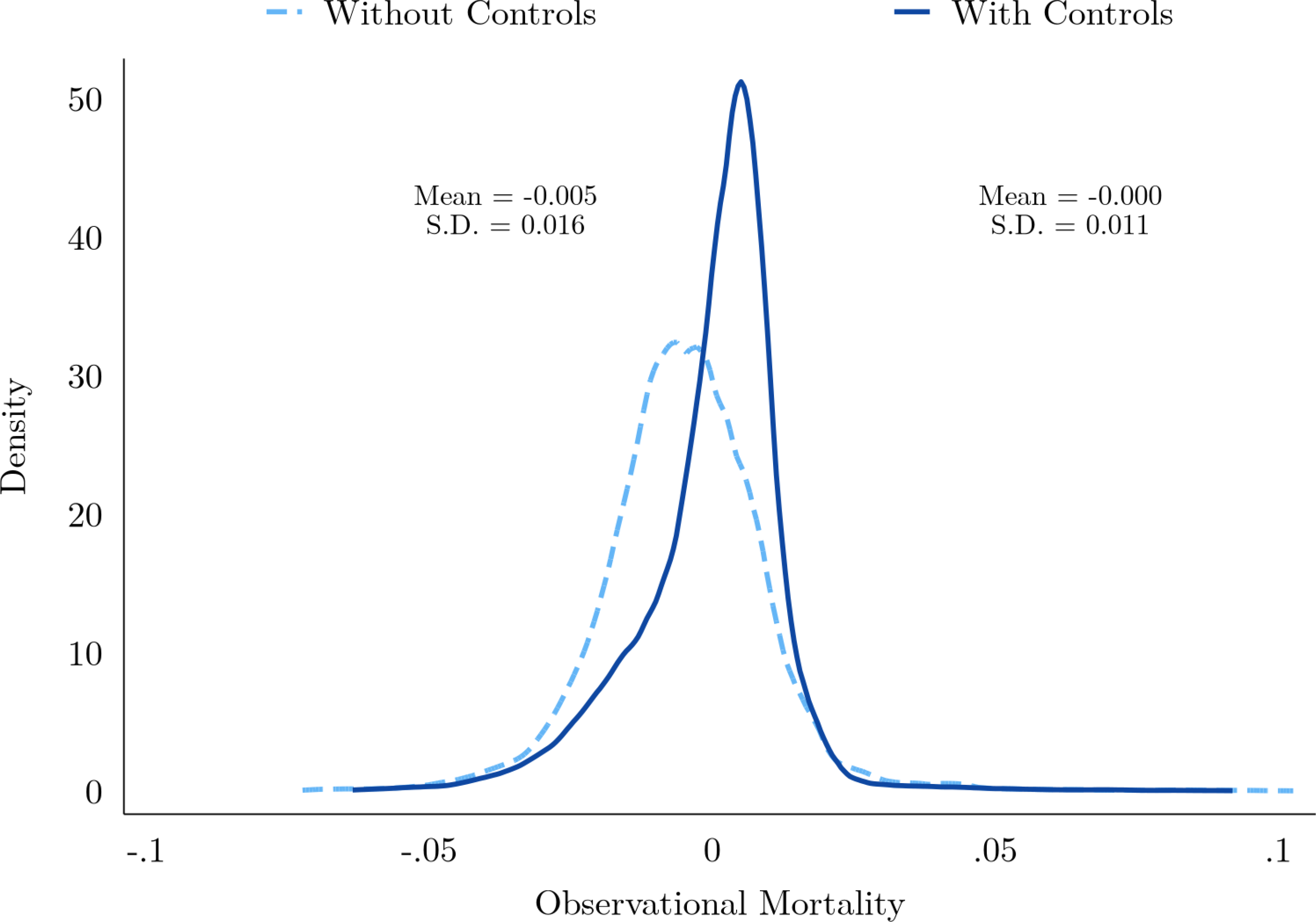
Estimates of Equation (1) reveal substantial within-county variation in MA plan mortality rates among observably similar beneficiaries. The estimated beneficiary-weighted standard deviation of μ_j across MA plans, after correcting for estimation error, is 1.1 percentage points or 23% of the average one-year mortality rate of 4.7%. Figure I plots the full distribution of shrunk observational mortality rates across MA plans. The solid line shows this distribution for our baseline specification of Equation (1), with all observable controls included in X_it, while the dashed line shows the corresponding distribution for a simpler specification that omits the beneficiary demographic controls. We normalize average observational mortality in both models by the average in the complete model that includes TM. The model without controls has a slightly lower mean (implying that MA plans have observably healthier beneficiaries than TM plans, on average) and a 45% larger standard deviation of 1.6 percentage points.

Figure I:

Observational Mortality

Notes: This figure summarizes the enrollment-weighted distribution of observational mortality across MA plans. The solid dark line shows this distribution when observational mortality is estimated from Equation (1), with all demographic controls, while the light dashed line shows the corresponding distribution for a simpler specification that omits age, race, sex, and dual-eligible status. Average observational mortality across all plans (TM and MA) is normalized to the average of the full model. Estimates are shrunk via the empirical Bayes procedure in Appendix C.1. Estimated means and standard deviations of μ_j for MA plans are for the prior distribution, computed as described in Appendix C.1, and shown for each estimation procedure.

The fact that the mean and standard deviation of observational mortality changes when beneficiary demographic controls are included suggests some degree of non-random selection. In other words, the variation in observational mortality from the simpler specification appears to be in part driven by observable differences in the health of plan enrollees and not the true mortality effects of plans. This selection appears to be primarily on two dimensions of our observable characteristics: age and dual-eligibility. Conditional on these characteristics, further controlling for beneficiary sex and race has little effect on the estimated distribution of observational mortality (e.g. the noise-adjusted standard deviation of μ_j remains at 1.1 percentage points). Absent further observables, we are unable to directly test for remaining selection bias in our benchmark specification.⁹ Instead, we derive an indirect validation based on termination-induced variation in MA choice sets.

2.4. Plan Terminations

To build intuition for our quasi-experimental approach to validating observational mortality, consider a set of beneficiaries who end a year enrolled in a MA plan with a high observational mortality rate μ_j. Since Medicare plan choice is highly inertial (only 14.1% of MA beneficiaries change plans in a given year, per Table I), most of these enrollees will remain in their high-mortality plan throughout the following year. Suppose, however, that at the end of the year the high-mortality plan terminates for a plausibly idiosyncratic reason (such as a federal change in reimbursement policy).

This termination would force the plan’s enrollees to make an active enrollment choice, and under standard regression-to-the-mean, they will tend to switch to a new MA plan that is more typical in terms of μ_j.¹⁰ If the observational mortality rates were causal, then all else equal we would expect the mortality of this enrollee cohort to fall commensurate to the decline in μ_j. Identical logic holds for beneficiaries enrolled in exogenously terminated plans with low observational mortality rates: subsequent plan choice is likely to be more typical in terms of μ_j, relative to enrollees in non-terminated low observational mortality plans. If observational mortality variation reflects causal effects, then mortality should rise. Combining these two termination quasi-experiments may reveal the predictive content of our observational mortality rate estimates while allowing for direct termination effects that are common to the high- and low-mortality terminations.

Figure II illustrates the relationship between plan mortality rates and termination status for high- and low-mortality plans in our IV sample. The solid lines indicate regression-adjusted trends in observational mortality for beneficiaries before and after a plan termination, separately for beneficiaries previously enrolled in plans with above-median (blue) and below-median (red) mortality.¹¹ The dashed lines indicate comparable trends in observational mortality for beneficiaries in the same counties and years whose plans did not terminate, again separately for beneficiaries enrolled in above- and below-median mortality plans. The solid lines indicate a regression-to-the-mean in plan choice following termination: those previously enrolled in high- and low-mortality plans tend to switch to more typical plans on average. At the same time, the dotted lines indicate inertia in plan choice absent termination: beneficiaries previously enrolled in high- and low-mortality plans tend to stay in these different plans provided they remain available. Bracketed 95% confidence intervals show that the post-termination difference in observational mortality is statistically significant for both high- and low-mortality plans, despite terminated and non-terminated plans having statistically indistinguishable observational mortality prior to termination.

Figure II:

Plan Terminations and Observational Mortality

Notes: This figure shows regression-adjusted trends in the observational mortality for enrollees in non-terminated and terminated MA plans, separately for plans with above- and below-median observational mortality. The median is defined over the entire IV sample. Data is plotted in the last year prior to termination for terminated plans and the following year. Termination effects are estimated in each year and median group by a separate regression which controls for county-by-year fixed effects; flexible interactions of lagged plan type and market shares; and beneficiary demographics (age in 5-year bands, sex, race and dual-eligibility status). County-clustered 95% confidence intervals for the termination effects are shown in brackets.

Figure III illustrates the corresponding relationship between realized beneficiary mortality and plans termination status for beneficiaries enrolled in high- and low-mortality plans. Here the solid and dashed lines correspond to the one-year mortality rates of the same groups of beneficiaries summarized in Figure II. Unlike the (time-invariant) observational mortality in Figure II, true mortality risk increases with age, such that the beneficiaries in non-terminated plans (dashed blue and red lines) exhibit an increasing trend in realized mortality. However, the solid blue line (indicating the realized mortality of beneficiaries enrolled in a low-mortality plan prior to termination) exhibits a steeper trend while the solid red line (indicating the realized mortality of beneficiaries enrolled in a high-mortality rate plan prior to termination) exhibits a decreasing trend. Again the bracketed 95% confidence intervals show a significant termination effect for both high- and low-mortality plans, with no statistically significant difference in average mortality prior to termination.

Figure III:

Plan Terminations and Beneficiary Mortality

Notes: This figure shows regression-adjusted trends in the one-year mortality of enrollees of non-terminated and terminated MA plans, separately for plans with above- and below-median observational mortality. The median is defined over the entire IV sample. Data is plotted in the last year prior to termination for terminated plans and the following year. Termination effects are estimated in each year and median group by a separate regression which controls for county-by-year fixed effects; flexible interactions of lagged plan type and lagged market shares; and beneficiary demographics (age in 5-year bands, sex, race and dual-eligibility status). County-clustered 95% confidence intervals for these effects are shown in brackets.

Together, the differential trends in Figures II and III suggest that a termination-induced move to MA plans with more typical observational mortality μj has a differential causal effect on actual mortality Y_it. This result suggests that the sizable variation in observational mortality we find in Figure I is not driven entirely by selection bias. At least some of the variation in observational mortality appears to be attributed to causal variation in MA plan mortality effects. We next develop an econometric framework to formalize this logic and measure the predictive validity of observational mortality for such causal effects.

3. Econometric Framework

We use an instrumental variables (IV) framework, leveraging plan terminations, to measure the validity of observational mortality differences in predicting differences in causal plan mortality effects. While not identifying mortality effects for individual plans, this approach is sufficient to estimate the expected mortality impact of reallocating beneficiaries across observably different plans. We first outline the econometric setting and parameter of interest before providing three conditions under which this parameter is identified by an IV regression. We devote special attention to the third condition, what we term the fallback condition, which is novel to this paper.

3.1. Plan Health Effects

We use a simple model to define causal plan effects and the IV parameter of interest. Let Y_ijt denote the potential mortality outcome of individual i in year t if she were to enroll in a plan j in her market. For the moment, we assume an additively separable model of Y_ijt =β_j +u_it; we extend our framework to account for unobserved treatment effect heterogeneity in Section 3.4 below. By normalizing the beneficiary-weighted average β_j in each market to zero, we can interpret each β_j as the average mortality effect from moving a random beneficiary to plan j, with u_it capturing latent differences in beneficiary health. Projecting u_it on a vector of observable characteristics X_it (which includes a constant) yields

$$Y_{ijt}={\beta }_j+X_{it}^{\prime }\gamma +{\epsilon }_{it},$$ (2)

where E[X_itε_it] = 0 by definition of the projection coefficient γ.

Consumers choose among the set of available plans in their market, with D_ijt = 1 indicating that consumer i enrolls in plan j in year t. Observed consumer mortality is then given by $Y_{it}={\sum }_j{Y}_{ijt}{D}_{ijt}$. Substituting in the previous expression for Y_ijt yields

$$Y_{it}=\sum _j{\beta }_j{D}_{ijt}+X_{it}^{\prime }\gamma +{\epsilon }_{it}.$$ (3)

In contrast to the regression model (1) in the previous section, Equation (3) is a causal model linking beneficiary plan choice D_ijt to subsequent mortality Y_it via the causal plan effects β_j.

Nonrandom plan selection creates fundamental econometric challenges in estimating plan mortality effects. To the extent that any given plan attracts consumers of poor (good) unobserved health, its observed mortality rate will be an upward- (downward-)biased estimate of β_j. For this reason, variation in the regression parameters μ_j that we estimate in Equation (1) need not coincide with variation in the causal parameters β_j in Equation (3): formally, average unobserved health ε_it need not be uncorrelated with the D_ijt choice indicators.

In principle, quasi-experimental variation in plan choice could be used to address such selection bias and estimate the full set of plan effects. This IV approach would require a set of exogenous variables Z_ijt to instrument for the plan choice indicators in Equation (3). In practice, any available quasi-experimental variation in plan choice is unlikely to generate enough instruments for such a procedure (given the large number of MA plans in each market) nor have sufficient power to detect small differences in mortality effects (since mortality is relatively rare). We next discuss our approach to quantifying variation in the plan mortality effects in light of these challenges.¹²

3.2. The Forecast Coefficient

Our first goal is to measure the relationship between observational mortality μ_j and true MA mortality effects β_j. Formally, we seek to estimate the MA forecast coefficient λ, defined by the projection of causal mortality effects β_j on observational mortality μ_j. Normalizing the means of both parameters to zero, this projection can be written

$${\beta }_j=\lambda {\mu }_j+{\eta }_j,$$ (4)

where η_j is mean-zero and uncorrelated with μ_j by definition. This regression is infeasible in the sense that the dependent variable β_j is neither observed nor estimated, despite measurement of the independent variable μ_j. The forecast coefficient nevertheless captures the predictive validity of the observational mortality measures. For example, μ_j is an on-average unbiased predictor of causal mortality effects when λ = 1, while observational mortality has little association with true causal effects when λ is small.¹³ We emphasize that Equation (4) reflects an equilibrium statistical relationship, given by existing patterns of selection, and that λ is not a structural parameter.

Along with the forecast coefficient, Equation (4) defines a forecast residual, η_j. This residual reflects the fact that for a given level of observational mortality μ_j, some plans may increase mortality by more or less than expected due to selection bias (even when λ = 1). Only when both λ = 1 and η_j = 0 for all j is observational mortality unbiased for individual MA plans (i.e. μ_j =β_j).¹⁴ Since Cov(η_j, μ_j)= 0, knowledge of the forecast coefficient is enough to place a lower bound on the variance in true causal effects, even in the presence of selection bias, by ignoring the contribution of η_j. Namely, Var(β_j) ≥ λ²Var(μ_j).

While it is not feasible to estimate Equation (4) directly, we can relate it to observed enrollee mortality via the causal model (3). Substituting the former equation into the latter, we obtain

$$Y_{it}=\lambda {\mu }_{it}+X_{it}^{\prime }\gamma +{\epsilon }_{it}+{\eta }_{it},$$ (5)

where ${\mu }_{it}={\sum }_j{\mu }_j{D}_{ijt}$ denotes the observational mortality of beneficiary i given her plan choice D_ijt and ${\eta }_{it}={\sum }_j{\eta }_j{D}_{ijt}$ is the corresponding forecast residual of her selected plan.

Equation (5) is again a causal model, linking observational mortality μ_it to realized mortality Y_it via the forecast coefficient λ. As with Equation (3), OLS estimation of Equation (5) will be biased when consumers of different unobserved health sort non-randomly into plans.¹⁵ To estimate the forecast coefficient, we instead use an IV approach that follows the logic of Figures II and III. This approach uses an instrument for the observational mortality of an enrollee’s plan that combines quasi-experimental choice set variation from plan terminations and the lagged observational mortality of an enrollee’s plan. In contrast to the initial causal model, a single valid instrument is enough to identify λ in Equation (5). There is, however, a cost to simplifying Equation (3), captured by the additional residual term η_it. We next discuss this cost in formalizing our IV approach.

3.3. Identification

Intuition and Related Literature

To see the basic logic of our IV approach, consider a market with three plans of equal market shares. Two of the plans, A and B, have an observational mortality of 0.05 and the third plan C has an observational mortality of 0.03. Suppose plan C exogenously terminates, and that subsequently all of its enrollees move to plan A or B. In either case, enrollees in plan C move to a plan where observational mortality is 2 percentage points higher. All else equal, the forecast regression (4) should then predict the resulting change in beneficiary mortality. If λ = 1, we expect mortality for the plan C cohort to rise by 5 − 3 = 2 percentage points. If instead λ = 1/2, we expect this cohort’s mortality to rise by $\frac{1}{2}(5-3)=1$ percentage point, as the 2 percentage point difference in observational mortality between plan C and either A or B would then partly reflect selection bias and not causal effects. Such intuition mirrors the motivation for quasi-experimental evaluations of observational quality measures in other settings (e.g. Kane and Staiger, 2008; Chetty, Friedman, and Rockoff, 2014; Angrist et al., 2016; Doyle, Graves, and Gruber, 2019).

A subtle but key ingredient to this intuition is “all else equal.” In the three-plan example, there is an implicit assumption that not only are terminations as-good-as-randomly assigned to plan C, in the sense of being unrelated to unobserved beneficiary health ε_i, but that the plans chosen before and after its termination are representative in terms of η_j, the error term in Equation (4). In fact, the presence of η_j may confound quasi-experimental inferences on λ, even when terminations are completely randomly assigned and thus independent of beneficiary health.

To see how the forecast residual can yield misleading quasi-experimental estimates of the forecast coefficient, suppose that while observational mortality is unbiased on average (λ = 1), there is still bias at the level of individual plans (η_j ≠ 0). Concretely, suppose in the three-plan example that β_A = β_C = 0.03 and β_B = 0.07. In this case the exact mixture of fallback plans A and B determines how mortality responds to the termination. If all enrollees move to plan B following plan C’s termination, then mortality will rise by 4 percentage points. Given the observational mortality difference of 2 percentage points, a naïve estimate of the forecast coefficient will be inflated by a factor of 2 (i.e.$\frac{{\beta }_B-{\beta }_C}{{\mu }_B-{\mu }_C}=2\lambda$). Conversely, if all of C’s enrollees switch to plan A, one might falsely conclude that observational mortality has no relationship with true causal effects (i.e.$\frac{{\beta }_A-{\beta }_C}{{\mu }_A-{\mu }_C}=0$). Only in the case where beneficiaries sort evenly into plans A and B following C’s termination, maintaining the equal market shares of the original plan choice distribution, will the comparison of actual mortality effects to observational mortality effects yield the correct estimate of λ = 1.

This potential challenge with quasi-experimental estimation of parameters like λ is quite general. For example, Doyle, Graves, and Gruber (2019) uses ambulance referral patterns to measure returns to hospital spending, implicitly relating a hospital’s average spending to its quality β_j. As they discuss, this approach requires more than random assignment of patients to ambulances. For their IV estimates to be unbiased, ambulance companies cannot systematically bring patients to higher quality hospitals conditional on spending. Similarly, Chetty, Friedman, and Rockoff (2014) consider the case of teachers quasi-randomly moving across schools. To recover a forecast coefficient for grade-level teacher value-added parameters β_j, they require an additional assumption. New schools cannot be systematically good conditional on observational value-added. Within schools, grade assignments further cannot track variation in value-added not captured by the observational measure.¹⁶

We next formalize a novel solution to this general issue. The formal challenge in such settings is that the usual instrument exclusion restriction comprises two distinct assumptions: a familiar balance condition (satisfied when the instrument is as-good-as-randomly assigned) and a novel condition restricting the fallback choices of individuals subjected to a quasi-experimental shock (such as plan terminations, ambulance company assignment, or teacher moves). Intuitively, in our setting, the choices following a plan termination cannot systematically differ across terminated plans in ways that are correlated with the forecast residual η_j.

This solution can be compared and contrasted with other strategies using shocks to institutional choices in order to estimate causal effects. Abowd, Kramarz, and Margolis (1999) famously estimate worker and firm premiums using a two-way fixed effects model. Their approach identifies firm-specific β_j under a parallel trends restriction, akin to that of difference-in-differences, which assumes workers moving between different firms j would have seen similar wage changes absent a move (Card et al., 2018; Hull, 2018). The two-way fixed effects approach differs from our IV approach—as well as the examples above—in which an external shock to movement decisions is used to relate an observed characteristic of j to the β_j’s, without restricting outcome trends. Gibbons and Katz (1992) use an approach more similar to ours in the wage premium literature. They use plausibly exogenous plant closings to relate the observed differences in wages of industries j to industry premiums β_j. Here a worker’s fallback industry following a plant closing need not be exogenous, and the authors test for this possibility. We provide a formal foundation for such an approach and propose new tests.

In our stylized example above, the fallback condition required that beneficiaries sort evenly into plans, which might suggest that this condition is generally quite strong. In fact, when pooling termination-induced choice set variation across many markets, the solution becomes weaker and more natural. We show below that the fallback condition holds in a wide range of discrete choice models (including those typically estimated in the industrial organization literature) and can be empirically investigated. Before presenting the general condition and its microfoundation, we first discuss the more standard first-stage and balance assumptions required by our IV approach.

The First-Stage and Balance Assumptions

Our approach to estimating the forecast coefficient uses an instrument which, as in Figures II and III, leverages the interaction of past plan choice and plan terminations. Consider, for a beneficiary i observed in year t, the instrument

$$Z_{it}={\mu }_{i,t-1}\times T_{i,t-1},$$ (6)

where μ_i,t−1 denotes the observational mortality of the beneficiary’s plan in the previous year, and T_i,t−1 is an indicator for whether that year was the plan’s last (prior to termination). We first derive conditions for this instrument to identify λ in a simplified setting where observational mortality is known without estimation error, there is no unobserved treatment effect heterogeneity, and we control only for characteristics of a beneficiary’s plan in the previous year (including μ_i,t−1 and T_i,t−1). We discuss how we relax each of these simplifying assumptions in Section 3.4 below.

An IV regression of beneficiary mortality Y_it on observational mortality μ_it which instruments with Z_it and controls for X_it identifies the forecast coefficient λ under three conditions, per Equation (5). First, we require that the residualized instrument ${\tilde{Z}}_{it}$ (that is, Z_it after partialling out X_it in the population) is correlated with observational mortality:

Assumption 1. (First Stage):$Cov\left({\tilde{Z}}_{it},{\mu }_{it}\right)\ne 0$.

The first-stage condition is highly intuitive in our setting. We expect most beneficiaries to remain in their previous year’s plan due to inertia, unless the plan is terminated. Beneficiaries forced into an active choice by a termination, however, will tend to switch to more typical plans. This combination of inertia and regression-to-the-mean implies that lagged terminations are likely to predict the observational mortality of year t choices differentially depending on lagged observational mortality, so that ${\tilde{Z}}_{it}$ and μ_it are negatively correlated. Such negative correlation is shown in Figure II, where terminated enrollees in below-median (above-median) observational mortality plans saw an increased (decreased) observational mortality of their enrolled plan in the following year.

The second condition is a standard balance assumption: that Z_it is conditionally uncorrelated with unobserved beneficiary health ε_it.

Assumption 2. (Balance):$Cov\left({\tilde{Z}}_{it},{\epsilon }_{it}\right)=0$.

As-good-as-random assignment of plan terminations is sufficient, but not necessary for this condition to hold. Since Z_it is given by the interaction of terminations and lagged observational mortality, and since both Z_it and X_it only vary at the lagged plan level, a minimal assumption is that any relationship between observational mortality and the average unobserved health of a plan’s beneficiaries is the same for terminated and non-terminated plans. Formally, we can evaluate Assumption 2 in terms of the infeasible plan-level difference-in-differences regression,

$${\overline{\epsilon }}_{jt}={\varphi }_Z\left({\mu }_j\times T_{j,t-1}\right)+X_{j,t-1}^{\prime }{\varphi }_X+e_{jt},$$ (7)

where ${\overline{\epsilon }}_{jt}=E\left[{\epsilon }_{it}\mid D_{ij,t-1}=1\right]$ denotes the average unobserved health among beneficiaries previously enrolled in plan j and X_j,t−1 includes the lagged plan characteristics in X_it (including the μ_j and T_j,t−1 main effects). Appendix C.2 shows that $Cov\left({\tilde{Z}}_{it},{\epsilon }_{it}\right)=0$ if and only if ϕ_Z = 0 in the version of this regression that weights by lagged market shares. Since T_j,t−1 is included in X_j,t−1, this formulation of Assumption 2 makes clear that we allow both for terminated and non-terminated plans to enroll beneficiaries of systematically different unobserved health, and for plan terminations to have direct disruption effects. We only require that this imbalance or effect is not systematically related to the observational mortality measure.¹⁷ The similarity of the pre-period mortality in Figure III supports the stronger version of Assumption 2 in our setting; we develop and apply additional falsification tests of the sufficient balance assumption in Section 4.1 below.

The Fallback Condition

The third identification condition we formalize is novel, and follows the above intuition regarding fallback plans. Even when terminations are as-good-as-randomly assigned (satisfying Assumption 2), consumers are not randomly assigned to fallback plans after terminations. Imbalance in the forecast residual η_j must thus be ruled out for Z_it to identify λ:

Assumption 3. (Fallback):$Cov\left({\tilde{Z}}_{it},{\epsilon }_{it}\right)=0$.

Recall that ${\eta }_{it}={\sum }_j{D}_{ijt}{\eta }_j$ is the forecast residual of the plan that consumer i selects in period t, potentially following a termination in time t −1. For the instrument to be relevant, ${\tilde{Z}}_{it}$ must be correlated with subsequent plan choice D_ijt; thus, the as-good-as-random assignment with respect to η_j does not guarantee that ${\tilde{Z}}_{it}$ is uncorrelated with η_it. Assumption 3 rules out this correlation, requiring fallback choices to be “typical” in a particular sense.

Interpreting Assumption 3 can be challenging because η_it is not structural. It instead arises from the statistical Equation (4) and the potentially complex realizations of consumer choices and health which give rise to μ_j. We take two approaches to better understand the fallback condition. First, we give a plan-level interpretation analogous to Equation (7). Second, we microfound the condition by asking what restrictions on consumer plan choices would cause it to hold.¹⁸

The fallback condition can be viewed (as with Assumption 2) as restricting the relationship between observational mortality and a particular plan-level unobservable to be similar across terminated and non-terminated plans. Specifically, Assumption 3 restricts a plan-level difference-indifferences regression which replaces ${\overline{\mathbf{\epsilon }}}_{jt}$ in Equation (7) with ${\overline{\eta }}_{jt}=E\left[{\eta }_{it}\mid D_{ij,t-1}=1\right]$. For the fallback condition to hold, the interaction of observational mortality μ_j and lagged plan termination T_j,t−1 must not predict ${\overline{\eta }}_{jt}$ conditional on the controls. This, in turn, says that the conditional relationship between μ_j and the average η_j of beneficiaries previously enrolled in terminated and non-terminated plans must be the same. This plan-level interpretation gives some intuition for the behavioral restrictions that might be sufficient. The fallback condition requires the first- and second-choice plans of consumers (i.e. the choices made before and after termination) to be similar, in terms of the relationship between the predictable dimension of plan quality μ_j and the unpredictable dimension η_j. Since the first-choice μ_j and η_j are uncorrelated by definition, the fallback condition requires that this lack of correlation remains as consumers switch from their first-choice plan to their second-choice plan. The fallback condition holds if consumers, after terminations, make similar choices from the remaining plans as new consumers in the market.

Microfounding the fallback condition requires behavioral restrictions on underlying consumer choice, since Assumption 3 is not ensured by as-good-as-random assignment of plan terminations. Appendix C.4 presents a discrete choice model that yields such restrictions. The simplest version of the model assumes that consumers in non-terminated plans are fully inertial, while consumers in terminated plans make an unrestricted choice that maximizes their latent utility U_ijt. We show that the fallback condition holds provided the IV control vector X_it includes any lagged characteristics of plans that lead to persistent unobserved heterogeneity in choice (along with μ_i,t−1 and T_i,t−1). Suppose, for example, that consumer utility has the form

$$U_{ijt}={\alpha }_{it}^{\prime }{W}_j+{\xi }_j+u_{ijt},$$ (8)

where α_it captures potentially heterogeneous preferences over observed plan characteristics W_j, ξ_j denotes a fixed plan unobservable, and u_ijt captures unobserved idiosyncratic time-varying plan-specific preferences. We show in Appendix C.4 that the fallback condition holds in this model (absent any functional form assumptions) when α_it is either fixed across consumers or idiosyncratic over time. For general α_it, we show that the fallback condition holds provided flexible transformations of the lagged plan characteristics W_j are controlled for: namely, when one conditions on the characteristics of plans over which consumers exhibit heterogeneous and persistent preferences. Similar logic can be extended outside the utility model of Equation (8): in Appendix C.4 we discuss how any controls sufficient to capture persistent heterogeneity in plan choice probabilities can be included to satisfy Assumption 3 more generally. We further show that consumers in non-terminated plans need not be fully inertial; the same logic can hold in models with partial inertia, such as that of Ho, Hogan, and Morton (2017).¹⁹

The microfoundation suggests the novel fallback condition is likely to hold in discrete choice specifications that are commonly estimated in both canonical and recent papers in the industrial organization literature. For example, Equation (8) is the classic random-coefficient model of demand for differentiated products used in Berry, Levinsohn, and Pakes (1995). More recently, Allende (2019) employs a model in this class when estimating school value-added. That said, there exist choice specifications that would violate the fallback condition. Assumption 3 could fail if, for example, termination-induced changes in preferences cause consumers to select plans differently.²⁰

The microfoundation of the fallback condition has two implications for our IV approach. First, when estimating the MA forecast coefficient it may be important to control for lagged plan characteristics over which consumers may have persistent heterogeneous preferences. We include such controls in our baseline specification, as discussed below. Second, as with the conventional balance assumption, the fallback condition may be investigated empirically. Assumption 3 asserts that the forecast error of a beneficiary’s plan, η_it, is conditionally uncorrelated with the instrument ${\tilde{Z}}_{it}$. We do not observe this residual directly, just as we do not observe the beneficiary residual ε_it which enters Assumption 2. However, just as standard IV falsification tests can investigate whether the instrument is correlated with observable proxies of ε_it, we can construct and test for instrument balance on an observable proxy for η_it. Intuitively, we would check whether the observable characteristics of a beneficiary’s fallback plans have a differential relationship with the observational mortality of her previous plan, across those previously enrolled in terminated and non-terminated plans. We conduct this test in the MA setting below.

3.4. Extensions

We consider four extensions to our basic econometric framework before bringing it to the data. First, we note that while we have derived the first-stage, balance, and fallback conditions for an IV regression involving μ_j, in practice the observational mortality of each plan is not known and must be estimated. We show in Appendix C.5 how each of these conditions extend to the case where μ_j is replaced with an empirical Bayes posterior mean of observational mortality ${\mu }_j^{*}$. The untestable balance assumption is unchanged in this case, while the feasible IV regression fallback condition is satisfied under the same microfoundation we considered above. Importantly, we continue to estimate the same forecast coefficient λ with the feasible IV regression as we would if observational mortality were known, although increased estimation error in ${\mu }_j^{*}$ is likely to reduce power. In practice the issue of estimating μ_j should be of little empirical consequence in our setting, since the typical plan in our sample has thousands of enrollees and the typical shrinkage coefficient is correspondingly close to one (see Appendix Figure A.II.).

Second, we note that we simplified the exposition by only considering an IV regression with lagged plan-level controls, of the form $X_{it}={\sum }_j{X}_{j,t-1}{D}_{ij,t-1}$. This restriction also allows for controls at a level higher than plan, such as county-by-year fixed effects. In practice we further include controls that vary at the beneficiary level (such as demographics) in some IV specifications. When not necessary for identification, we expect such controls to absorb residual variation in beneficiary mortality and potentially yield precision gains.

Third, in Appendix C.6 we show how our framework can accommodate unobservable selection on heterogeneous treatment effects. Our core argument proceeds similarly, although we require a further condition on unobserved selection on treatment effects. The new condition requires that any relationship between the degree of such “Roy selection” and observational mortality is again the same among consumers in terminated and non-terminated plans. Below we probe the role of treatment effect heterogeneity by allowing plan effects to vary by observables.

Finally, we note that while we have derived first-stage, balance, and fallback conditions for the purposes of estimating the forecast coefficient λ, analogous conditions can be imposed to estimate the coefficient from regressing plan effects β_j on any plan observable W_j. The first stage for an instrument of the form Z_it =W_i,t−1×T_i,t−1 (where $W_{i,t-1}={\sum }_j{W}_j{D}_{ij,t-1}$) continues to derive power from a combination of plan choice inertia and termination-induced regression-to-the-mean; the balance assumption is analogous to Assumption 2, and the appropriate fallback condition continues to hold under our choice model microfoundation. We use this extension in Section 5 to study the observable correlates of plan quality, such as premiums and star ratings. We also show how our IV framework can be used to bound the implicit willingness to pay for plan quality using the association between plan mortality effects and premium-adjusted market shares.

4. Results

4.1. Tests of Assumptions

We first investigate Assumption 1 by showing that termination-induced changes to consumers’ choice sets lead to predictable changes in the observational mortality of the plan in which they subsequently enroll. We show this by estimating an OLS first-stage regression of

$${\mu }_{it}={\pi }_Z{Z}_{it}+X_{it}^{\prime }{\pi }_X+v_{it},$$ (9)

where again μ_it denotes the plan observational mortality for beneficiary i at time t and Z_it = μ_i,t−1× T_i,t−1 is the interaction of observational mortality of the lagged plan and an indicator for lagged plan termination. To explore robustness, we sometimes replace the linear interaction with more flexible alternatives, such as interactions of percentiles of lagged observational mortality and lagged plan terminations. The baseline control vector X_it includes county-by-year fixed effects (such that we only exploit variation within choice sets), year- and county-specific termination main effects (to allow for flexible direct effects) and flexible interactions of lagged plan type, lagged observational mortality, and lagged plan size and market shares (to allow for a weakened fallback condition).²¹

In some specifications we also include controls for beneficiary demographics (age in 5-year bands, sex, race and dual-eligibility status). We cluster standard errors at the county level, allowing for arbitrary correlation in the regression residual across different beneficiaries, plans, and years.²²

First-stage coefficient estimates are reported in Panel A of Table II. The finding of π_Z < 0 is consistent with a combination of inertia and regression-to-the-mean in MA plan choice, first documented in Figure II. Beneficiaries enrolled in high- or low-mortality plans that are terminated in year t −1 tend to choose plans in year t which are more typical in terms of observational mortality, relative to the mostly inertial beneficiaries in non-terminated plans; consequently, ${\tilde{Z}}_{it}$ and μ_it are negatively correlated. In column (1), we estimate a termination-induced regression-to-the-mean of −0.72, implying that a consumer in a one percentage point higher observational mortality plan in the previous period switches to a plan with 0.72 percentage points lower observational mortality in the period following termination, relative to a consumer in a similarly high-mortality plan that does not terminate. Column (2), corresponding more directly to Figure II, shows that the termination of an above-median observational mortality plan in year t − 1 induces a differential reduction in the observational mortality of year t plans of 0.02 percentage points, relative to a termination of a below-median observational mortality plan. Both specifications yield high first-stage F statistics, confirming the relevance of our instrument (Assumption 1).

Table II:

Tests of Assumptions

	(1)	(2)
Dep. Var.: Observational Mortality	A. First Stage
Instrument	−0.724 (0.015)	−0.0189 (0.0014)
F Statistic	2,358.1	173.9
Dep. Var.: Predicted Mortality	B. Balance
Instrument	−0.020 (0.013)	−0.0011 (0.0006)
Dep. Var.: Predicted Forecast Residual	C. Fallback
Instrument	0.010 (0.001)	−0.0000 (0.0001)
Specification	Linear	Median
Demographic Controls	No	No
N Beneficiary-Years	11,441,205

Notes: Panel A of this table is based on estimation of Equation (9) and presents the OLS coefficient in a first-stage regression of observational mortality on the instrument. Panel B replaces observational mortality as the dependent variable with a prediction of one-year mortality based on beneficiary demographics. Panel C uses as the dependent variable a prediction of the forecast residual based on plan characteristics. In column (1) the instrument is the interaction of observational mortality of the lagged plan and a lagged plan termination indicator. In column (2) the instrument is the interaction of an indicator for above-median observational mortality of the lagged plan and a lagged plan termination indicator. In all specifications, we control for the observational mortality of the lagged plan and termination main effects, county-by-year fixed effects, year- and county-specific termination effects, and interactions of lagged plan characteristics (as described in the text). Standard errors are clustered by county and reported in parentheses.

Panel A of Figure IV illustrates the first-stage relationship by replacing the linear instrument in Equation (9) with one based on deciles of lagged observational mortality (controlling for decile main effects). We use this specification to plot the estimated contemporaneous plan observational mortality for enrollees who, in the previous year, were enrolled in plans of different deciles of observational mortality that did and did not terminate. The figure shows that while observational mortality of the lagged plan predicts current plan observational mortality among the non-terminated group, the relationship is essentially flat for terminated plans. The flattening again reflects the combination of inertia and regression-to-the-mean in plan choice that yields negative first-stage coefficients in Panel A of Table II.²³

Figure IV:

Graphical Tests of Assumptions and the Reduced Form

Notes: This figure illustrates the three assumptions in our IV approach, as well as the IV reduced form. Panel A shows average observational mortality by deciles of lagged observational mortality among non-terminated and terminated plans, controlling for county-by-year fixed effects and other observables in our baseline specification. Panel B shows the corresponding averages of predicted one-year mortality given omitted beneficiary demographics (age, sex, race, and dual-eligible status). Panel C shows the corresponding averages of a predicted forecast residual given omitted plan characteristics (star ratings, premiums, MLRs, and an indicator for donut hole coverage). Panel D shows the corresponding averages of one-year mortality. Points are the average of each left-hand side variable in deciles of lag plan observational mortality, predicted by the lagged observational mortality in the regression model, combined with the decile-specific termination effects estimated from specifications of the form of Equation (9). The controls as in Table II, including decile main effects. Coefficients are normalized to remove termination main effects.

We next build support for the balance condition (Assumption 2) by testing whether the instrument predicts observable differences in beneficiary health. We replace the observational mortality outcome in Equation (9) with a prediction of one-year beneficiary mortality, obtained from a regression of one-year mortality on dummies for 5-year age bands, sex, race, and dual-eligibility fixed effects (see Appendix Table A.III. for model estimates). The results are in Panel B of Table II. In contrast to the large and significant first-stage effects in Panel A, we cannot reject the null of instrument balance on predicted beneficiary mortality. With the baseline linear specification we obtain an insignificant coefficient of −0.020, while in the median specification we obtain an insignificant coefficient of −0.0011. Both of these estimates are more than an order of magnitude smaller than the corresponding first-stage estimates. Finding balance for our instrument on predicted mortality is not surprising in light of the motivating Figure III.

Panel B of Figure IV illustrates the predicted mortality regressions by replacing the observational mortality measure in Panel A. We plot the average predicted mortality among terminated and non-terminated plans at different deciles of lagged observational mortality. In contrast to the clear first-stage effect, there is no differential trend in predicted mortality for terminated versus non-terminated plans. Any differential trend in the actual mortality of beneficiaries in terminated and non-terminated plans is therefore unlikely to be due to pre-existing differences in their health.

Appendix Figure A.III. similarly shows that our instrument appears visually balanced on age and average CMS risk scores, which attempt to predict enrollee costs based on demographics and diagnoses. Additional balance tests are given in Appendix Table A.IV..²⁴

Finally, we build support for the novel fallback condition (Assumption 3) by testing whether our instrument predicts an observable proxy for the forecast residual η_i. We construct the proxy by first regressing observational mortality on a set of observable plan characteristics (plan star ratings, premiums, medical loss ratios, and an indicator for donut hole coverage). We then take the residual from projecting the fitted values from this regression (as an observable proxy of β_j) on μ_j. This residual yields an observable proxy for η_j, and thus of ${\eta }_i={\sum }_j{\eta }_j{D}_{ij}$ given a beneficiary’s plan. Panel C of Table II reports the resulting instrument coefficients from replacing the outcome in Equation (9) with this proxy. In this case, we find a coefficient of 0.01 in the linear specification and a coefficient of effectively zero in the median specification. While statistically significant, the linear imbalance is quantitatively negligible—almost two orders of magnitude smaller than the associated first-stage effect. In Appendix C.7, we show how the frameworks of Altonji, Elder, and Taber (2005) and Oster (2019) can be adopted to quantify the importance of imbalances on both beneficiary and plan-level observables. The statistical imbalances are too small to substantially alter our forecast coefficient estimates, even under conservative assumptions.

Panel C of Figure IV illustrates these predicted forecast residual regressions by replacing the predicted mortality measure in Panel B. As before, we see no systematic relationship between terminations and the predicted enrollee unobservable at any decile of lagged observational mortality. This result builds confidence in our third and final identification condition, suggesting that termination-induced changes in observational mortality can be related to termination-induced changes in actual mortality to estimate the MA forecast coefficient. We next present these IV estimates.

4.2. Forecast Coefficient Estimates

Table III reports first-stage, reduced-form, and second-stage estimates for our main IV specification. The second-stage estimates come from a regression of

$$Y_{it}=\lambda {\mu }_{it}+X_{it}^{\prime }{\gamma }_X+{\epsilon }_{it}+{\eta }_{it},$$ (10)

with the first stage given by Equation (9). The second-stage coefficient λ estimates the observational mortality forecast coefficient under Assumptions 1–3. The reduced form regression replaces the observational mortality outcome in Equation (9) with the actual mortality outcome in Equation (10). As before, we use both this linear specification and an alternative specification which replaces the instrument with one constructed from an above-median lag observational mortality indicator. We also report two specifications for the control vector X_it; one which mirrors the tests of our assumptions, and a second which adds beneficiary demographics (age, sex, race, and dual-eligible status). Given the balance of our instrument on these beneficiary observables, via the predicted mortality measure, we do not expect the inclusion of these controls to meaningfully affect the IV estimates (though it may increase their precision).

Table III:

Forecast Coefficient Estimates

	(1)	(2)	(3)	(4)
Dep. Var.: Observational Mortality	A. First Stage
Instrument	−0.724 (0.015)	−0.0189 (0.0014)	−0.724 (0.015)	−0.0189 (0.0014)
F Statistic	2,358.1	173.9	2,358.7	173.6
Dep. Var.: One-Year Mortality	B. Reduced Form
Instrument	−0.764 (0.069)	−0.0214 (0.0025)	−0.745 (0.069)	−0.0203 (0.0023)
Dep. Var.: One-Year Mortality	C. Second Stage (Forecast Coefficient)
Observational Mortality	1.056 (0.098)	1.130 (0.117)	1.029 (0.098)	1.073 (0.106)
Specification	Linear	Median	Linear	Median
Demographic Controls	No	No	Yes	Yes
N Beneficiary-Years	11,441,205

Notes: Panels A and C of this table report first- and second-stage coefficient estimates from Equations (9) and (10). Panel B reports the corresponding reduced-form coefficients. The dependent variable is observational mortality in Panel A and realized mortality in Panels B and C. In columns (1) and (3) the instrument is the interaction of observational mortality of the lagged plan and a lagged plan termination indicator. In columns (2) and (4) the instrument is the interaction of an indicator for above-median observational mortality of the lagged plan and a lagged plan termination indicator. In all specifications, we control for lagged observational mortality and termination main effects, county-by-year fixed effects, year- and county-specific termination effects, and interactions of lagged plan characteristics (as described in the text). Columns (3) and (4) additionally control for beneficiary demographics. Standard errors are clustered by county and reported in parentheses.

Panel A of Table III replicates the first-stage results reported in Panel A of Table II and confirms that these change little when we add the demographic controls. Panel B shows the corresponding reduced-form estimates from the same specifications. We find reduced-form coefficients of −0.76 and −0.75 for the linear specification (without and with demographic controls) and of −0.0214 and −0.0203 for the median specification. Each of these estimates are quite similar to the corresponding first-stage coefficients, reflecting the pattern first shown in Figures II and III: terminations tend to shift observational mortality and realized mortality by similar amounts.

Panel C of Table III shows that the similarity of first-stage and reduced-form effects yields high forecast coefficient estimates, in the range of 1.029–1.130, with standard errors in the range of 0.098–0.117. The point estimates are again similar with and without demographic controls, which reduce standard errors slightly. The median specification yields a somewhat higher forecast coefficient, though the estimates are not statistically distinguishable. Together, these IV estimates suggest the variation in observational mortality unbiasedly predicts variation in true mortality effects (i.e. that λ ≈ 1).

Panel D of Figure IV illustrates this finding by plotting reduced-form variation in one-year mortality rates for beneficiaries in terminated and non-terminated plans by deciles of lagged observational mortality. The resulting differential trend (obtained by replacing observational mortality in Equation (9) with actual one-year mortality) strongly mirrors that of the first stage in Panel A, consistent with the finding of a forecast coefficient that is close to one. Lagged observational mortality strongly predicts the subsequent mortality of beneficiaries previously enrolled in non-terminated plans, but this relationship is effectively flat for beneficiaries previously enrolled in terminated plans (who switch to more typical plans). This finding is striking in contrast to Panel B of Figure IV, which shows no such relationship for predicted one-year mortality. Beneficiaries in high- and low-mortality terminated plans appear similar to those in corresponding non-terminated plans until they are induced by terminations to choose more average plans.²⁵

4.3. Robustness Checks

We verify the robustness of our forecast coefficient estimates in a number of exercises summarized in Appendix Table A.VI.. First, we show that the estimates in Table III are unaffected by the removal of counties which do not see a plan termination during our sample period. The first row of Appendix Table A.VI. shows we obtain similar forecast coefficient estimates of around 1.00–1.05 in this specification, with comparable standard errors. This finding is consistent with the fact that the vast majority of counties see MA plan terminations (see Appendix Figure A.I.) and that counties with and without terminations are broadly similar (see Appendix Table A.I.).

Second, we verify that similar results are obtained when we drop the minority of beneficiaries who switch from a MA plan to a TM plan (our baseline specification includes comparisons between the majority of MA plans and a single TM plan in each county). While this specification may be biased by selecting on an endogenous variable, we nevertheless obtain similar forecast coefficients in the second row of Appendix Table A.VI..

Third, we show that we obtain similar but less precise estimates when we limit attention to terminations of PFFS plans. Pelech (2018) links such terminations to a 2008 policy change which increased PFFS operating costs. While these plan terminations are perhaps more plausibly exogenous, there may also be less variation across PFFS plans, which typically do not establish restrictive networks. The third row of Appendix Table A.VI. shows that these plan terminations yield a similar forecast coefficient estimate of 1.08, with a standard error of 0.11. The corresponding median specification gives a slightly larger but similar estimate, with a similar standard error. The fourth row of Appendix Table A.VI. reports the results of excluding PFFS terminations. Forecast coefficient estimates from this specification are more imprecise, but qualitatively similar to (and not statistically distinguishable from) our baseline estimates.

We next investigate the role of treatment effect heterogeneity. The fifth row of Appendix Table A.VI. shows that we obtain similar estimates, of around 1.05, when we exclude dual-eligible beneficiaries from both the IV sample and the sample used to construct the observational mortality measure. The sixth row further shows that our results are similar when we allow observational mortality to vary by beneficiary age, estimating Equation (1) separately by five-year age bins. This specification yields forecast coefficients of around 1.03–1.07, with similar or slightly smaller standard errors. This robustness is especially striking as age and dual-eligible status appear to drive the majority of selection bias in the most naïve observational mortality estimates, as discussed in Section 2.3. The findings suggest either that treatment effect heterogeneity is not first-order in this setting, or that the extension of our framework in Appendix C.6 (that accommodates such heterogeneity) is likely to hold.

We conclude this section by summarizing a number of additional robustness checks in Appendix Table A.VI.. We find similar results in the seventh row when including lagged plan risk scores as a control, consistent with the visual balance in Appendix Figure A.III.. We also find in the eighth row qualitatively similar (but slightly smaller) results when not shrinking the observational mortality estimates, consistent with the fact that the typical estimate is precise (per Appendix Figure A.II.) and the discussion in Appendix C.5. We further confirm in the ninth row that similar estimates of λ are obtained when dropping the smallest plans from our sample, which are likely to be the most imprecisely estimated. Finally, in the tenth row we report similar forecast coefficient estimates when using two-year mortality to both construct and validate observational mortality. This suggests observed differences in plan mortality rates can be highly predictive of true plan causal effects at different horizons of beneficiary mortality.

4.4. Interpretation

Taken together, our forecast coefficient estimates suggest that a large proportion of the sizable variation in observational mortality across MA plans reflects the causal impact of plan enrollment. It is worth emphasizing that this finding does not rule out selection bias in observational mortality, in the sense of μ_j ≠ β_j. Instead, our findings imply that variation in μ_j unbiasedly predicts variation in β_j, on average, despite any such selection bias. One might, for example, expect unobservably sicker beneficiaries to systematically prefer certain plans with more coverage. Our results and framework allow for this possibility: in the microfoundation of our fallback condition (discussed in Appendix C.4), we allow beneficiary preferences to correlate with their health in both observed and unobserved ways, nesting common discrete choice models of plan choice. A forecast coefficient near one can arise in such models even with systematic unobserved selection if the selection bias is negatively correlated with true causal effects (i.e. better plans attract unobservably sicker beneficiaries).²⁶ In this case (with η_j ≠ 0), our forecast coefficient estimates give a lower bound on the variability of true causal effects: with λ ≈ 1, the standard deviation of β_j is at least as large as the 1.1 percentage point standard deviation of μ_j found in Section 2.3.

While an effect size this large may seem surprising, it is broadly consistent with a growing literature that shows large impacts of insurance status on health outcomes. Medicare as a whole has been found to have large mortality effects. Card, Dobkin, and Maestas (2008), for example, estimate a 20% mortality reduction in Medicare beneficiaries who are admitted to emergency departments.²⁷ The literature on place-based mortality effects estimates similarly large variation within Medicare across all elderly beneficiaries, though these may capture both the joint impact of changing health systems and other demand side factors.²⁸ Below, we further argue that evidence on provider effects is consistent with the magnitudes we document.

5. Correlates of Plan Effects

When combined with our observational mortality estimates, a forecast coefficient close to one implies large differences in causal mortality effects across plans. In this section, we investigate how these differences relate to observed plan attributes. We first ask whether plan characteristics predict observational mortality, μ_j. We then extend our basic IV framework to see whether these characteristics predict true mortality effects β_j. We consider different characteristics that may serve as proxies of plan quality, capture financial generosity and potential mechanisms, or measure consumer willingness to pay for plan health effects.

5.1. Proxies of Plan Quality

We start by considering whether existing plan quality measures (star ratings) or prices (premiums) proxy for observational mortality and true plan effects. To help beneficiaries select plans, CMS produces star ratings on a 1–5 scale, with 5 stars indicatindicates hering the highest quality. Star ratings depend on consumer satisfaction surveys and measures of clinical quality, but they explicitly do not condition on outcome data like mortality. In addition to making these ratings available to consumers, the government now pays “bonuses” to highly rated (4- and 5-star) plans.²⁹

Surprisingly, we find that CMS star ratings are positively correlated with our observational mortality measure, suggesting higher-ranked plans have higher mortality rates.³⁰ The first column of Table IV, Panel A, shows that a one-star increase in a plan’s ratings is associated with a 0.08 percentage point increase in observational mortality, controlling for county-by-year fixed effects and other baseline controls. This is a small but statistically significant positive correlation. Of course, this correlation could arise either because higher-ranked plans have worse mortality effects β_j or because sicker beneficiaries sort into higher star rating plans (causing selection bias μ_j −β_j to be positively correlated with star ratings).

Table IV:

Plan Characteristics Regressions

	(1)	(2)	(3)	(4)	(5)
	Panel A: OLS (Observational Mortality)
Star Rating	0.0008 (0.0003)
Premium		0.0043 (0.0003)			0.0053 (0.0004)
Has Donut Hole Coverage			−0.0022 (0.0003)		−0.0031 (0.0003)
Medical Loss Ratio				0.0019 (0.0023)	0.0002 (0.0024)
	Panel B: IV (Plan Mortality Effect)
Star Rating	−0.0011 (0.0012)
Premium		−0.0058 (0.0019)			−0.0053 (0.0024)
Has Donut Hole Coverage			−0.0046 (0.0016)		−0.0004 (0.0022)
Medical Loss Ratio				−0.0136 (0.0058)	−0.0127 (0.0058)
First-Stage F Statistic	5,054.7	5,711.3	1,785.5	164.2	587.0
Maximum Forecast R2	0.0013	0.0267	0.0242	0.0048	0.0302
N Beneficiary-Years	11,441,205

Notes: This table reports OLS and IV estimates of the regression of observational mortality and plan mortality effects, respectively, on plan characteristics. The dependent variable is observational mortality in Panel A and one-year mortality in Panel B. All specifications include the baseline controls in columns (3) and (4) of Table III. The IV specifications instrument by the interaction of lagged plan characteristics and terminations, controlling for main effects. Premiums are monthly and measured in hundreds of dollars. Missing plan characteristics are replaced by the average non-missing value across plans. Standard errors are clustered by county and reported in parentheses. The maximum forecast R² is computed using the lower bound of Var(β_j) implied by the observational mortality forecast coefficient in column (3) of Table III.

To address selection bias, we next recover the relationship between true mortality effects, β_j, and star ratings by an extension of our IV approach. We estimate the analog of Equation (10),

$$Y_{it}=\theta W_{it}+X_{it}^{\prime }\rho +{\epsilon }_{it}+{\eta }_{W,it},$$ (11)

which replaces the observational mortality treatment μ_it with a measure $W_{it}={\sum }_j{W}_j{D}_{ijt}$ of a different enrolled plan characteristic W_j (here, star ratings), instruments with Z_it =W_i,t−1 ×T_i,t−1, and replaces lagged observational mortality in X_it with the lagged plan characteristic W_i,t−1. For star ratings, the IV coefficient θ intuitively captures the extent to which termination-induced switches from low-rated plan to high-rated plans correlate with increased mortality Y_it. Formally, we can interpret θ as the plan-level regression analogous to Equation (4) (which here projects plan effects β_j on star ratings W_j, instead of observational mortality μ_j) by natural extensions of our first stage, balance assumption and fallback conditions to this setting.

IV estimates of θ show no relationship between star ratings and mortality effects. The first column of Panel B in Table IV shows that a one-unit increase in star ratings is associated with a small and statistically insignificant 0.11 percentage point decrease in plan effects, with a standard error of 0.12 percentage points. This result suggests that the most commonly used measure of plan quality does not predict which plans systematically reduce beneficiary mortality on average.

We next investigate the correlation of observational mortality and plan effects with plan premiums. Premiums may also proxy for plan quality if quality investments are costly to insurers or if consumers demand higher quality plans (we investigate the latter in more depth in Section 5.3 below). In the second column of Panel A in Table IV we find a positive and highly significant relationship between premiums and observational mortality, suggesting that a $100 increase in monthly premiums is associated with a 0.43 percentage point increase in μ_j. Of course, as with star ratings, this correlation may be due to selection bias: plans may charge high premiums precisely because they enroll sicker-than-average beneficiaries.

IV estimates of the premium forecast coefficient are negative, suggesting that more expensive plans are of higher quality. The second column of Panel B in Table IV suggests that a $100 increase in monthly premiums ($1,200 per year) is associated with a 0.58 percentage point decrease in β_j. In combination with the OLS estimate, this finding suggests that higher premium plans are favored by sicker consumers (consistent with the findings of Starc (2015)). It also suggests that consumers may be leaving money on the table when it comes to the effective price of mortality reductions, a point we return to below. Even with conservative assumptions on the value of a statistical life, the dollar-equivalent mortality benefits of higher premium plans appears to exceed the added cost.³¹

Although premiums (in contrast with star ratings) significantly predict plan mortality effects, they still explain a small share of quality variation. Since we can use the observational mortality variance and forecast coefficient to place a lower bound on the variance of β_j, we can use the star rating and premium forecast coefficients to place an upper bound on the R² from regressing plan effects on either of these plan characteristics.³² We find a maximum R² of 0.001 for star ratings and 0.027 for premiums, suggesting that only a small share of within-market quality variation can be explained by either observable.

We emphasize that these IV results are causal in a limited sense. They do not imply that, for example, a plan which raises premiums will improve its quality. This stronger claim (that we have recovered the causal impact of plan characteristics on β_j) only follows under stronger assumptions. Namely, it would require that there are no omitted plan characteristics that are correlated with premiums and also impact mortality (such that the regression of β_j on plan characteristics is itself causal). However, our results do suggest that higher premium plans are of systematically higher quality, and are more predictive of quality differences than CMS star ratings. To further explore potential mechanisms for plan quality differences, we next turn to other plan characteristics.

5.2. Mechanisms

We investigate three mechanisms through which plans may impact beneficiary health: cost-sharing, direct control of beneficiary utilization, and provider networks.

We first study the potential role of cost-sharing, as proxied by whether a plan offers coverage in the Medicare Part D “donut hole” (a range of prescription drug expenditures at which some plans stop cost-sharing). In Panels A and B of Table IV we find that plans which offer donut hole coverage tend to both have lower observational mortality (0.2 percentage points) and significantly more negative plan effects (0.5 percentage points), on average. This contrast is consistent with earlier findings that sicker beneficiaries tend to select into plans with donut hole coverage (e.g. Polyakova (2016)).³³ The finding of large plan effect differences among plans which offer donut hole coverage suggests that lower cost-sharing may be more broadly beneficial.³⁴

MA plans may also affect utilization through other means, such as prior authorization requirements or physician reimbursement (Dillender, 2018). These supply side controls could affect both utilization and quality. We next study whether mortality effects correlate with overall expenditures, as measured by medical loss ratios (MLRs): the percentage of premiums which are paid out in claims.³⁵ In Panels A and B of Table IV we find that plans with higher MLRs tend to have higher observational mortality, but significantly lower plan effects. A ten percentage point increase in MLR is associated with a 0.14 percentage point reduction in the plan mortality effect, and we estimate a comparable coefficient if we condition on premiums. This finding suggests that expenditure levels predict plan quality, echoing a similar correlation found between hospital expenditure and mortality effects (e.g. Doyle et al. (2015)), but that sicker beneficiaries tend to be found in plans with higher loss ratios.

Finally, we relate our findings to estimates of provider heterogeneity. The existing literature documents large variation in hospital mortality effects (Hull, 2020; Doyle et al., 2015; Geweke, Gowrisankaran, and Town, 2003), with Hull (2020) and Doyle et al. (2015) finding evidence that such variation is reliably captured by observational models. Correspondingly, we find that a hospital observational mortality model estimated across all Medicare beneficiaries (with the same demographic controls) suggests a one standard deviation better hospital decreases one-year mortality by roughly 20%. Given the significant variation in provider networks across plans (e.g. Chernew et al. (2004)) this variation suggests a plausible mechanism for the equally large variation that we find in plan-level mortality effects. However an IV analysis of this potential mechanism is infeasible, given limited data on MA networks.³⁶

Overall, this analysis of mechanisms paints a clear and consistent picture. More expensive and higher spending plans tend to reduce beneficiary mortality while also tending to attract sicker beneficiaries. Still, much of the variation in plan quality remains unexplained as shown by the relatively low maximum R² of 0.0302 in column (5) of Table IV, which includes all financial measures.³⁷ The large residual variation leaves ample room for alternative but harder-to-measure channels, such as physician and hospital networks, to play an important role.

5.3. Demand for Plan Quality

We next estimate the extent to which higher quality plans tend to attract a greater market share. This analysis follows a further extension of our IV framework which allows us to estimate the implicit weight consumers place on plan mortality effects and estimate the implicit willingness to pay (WTP) for plan quality. Intuitively, we can estimate latent demand from a plan’s market share after accounting for differences in prices. Our IV framework then allows us to relate demand to unobserved plan quality and recover the WTP from this relationship.

To formalize our approach, first consider how WTP might be computed if plan quality β_j were directly observed. A standard discrete choice approach specifies consumers as selecting plans to maximize their latent utility U_ij, given by

$$U_{ij}=\alpha p_j+{\xi }_j+u_{ij},$$ (12)

where p_j denotes the observed premium of plan j, ξ_j collects all other relevant characteristics of plans (observed or unobserved by the econometrician), and u_ij is a set of unobserved taste shocks for consumer i. We follow the usual assumption that u_ij follows a type-I extreme value distribution but make no other parametric assumptions and allow premiums to be endogenous in the sense of being correlated with ξ_j. Projecting ξ_j on β_j across plans, we obtain a decomposition of ξ_j = τβ_j +ψ_j with ψ_j uncorrelated with β_j. We expect both α and τ to be negative, as both higher premiums and larger mortality effects (worse quality) will tend to decrease demand. The ratio τ/(100×α) captures the WTP for plan quality: the decrease in premiums sufficient to offset a one percentage point increase in mortality effects β_j, on average across other characteristics ψ_j.

When p_j and β_j are both observed, standard discrete choice methods (e.g. Berry (1994)) may be used to estimate the WTP parameter, perhaps using instruments to account for the possible endogeneity of premiums with respect to β_j and ψ_j. In practice β_j is not known; we instead observe the unbiased prediction $\lambda {\mu }_j^{*}$, where λ is again the observational mortality forecast coefficient (approximately one, in this setting) and ${\mu }_j^{*}$ is posterior observational mortality. Naïvely using this proxy in discrete choice estimation of WTP is likely to generate bias for at least two reasons. First, estimation error in ${\mu }_j^{*}$ (due to finite samples) is likely to bias estimates of τ and α, potentially in the direction of attenuating the WTP estimate. Second, even when λ = 1, there may be unobserved differences in quality (i.e. non-zero η_j) that may add further bias of ambiguous sign.³⁸

We employ an alternative WTP estimation procedure that combines the discrete choice formulation with our IV framework for estimating plan forecast coefficients. Equation (12) implies that variation in log plan market shares recovers the normalized systematic component of consumer utility, which we denote δ_j:

$$ln\left(s_j\right)-ln\left(s_0\right)={\delta }_j\equiv \alpha p_j+\tau {\beta }_j+{\psi }_j,$$ (13)

where we have without loss normalized the plan characteristics as relative to an outside option with market share s₀. Given an estimate or calibrated value of the premium coefficient α, we may back out from this expression ξ_j = δ_j −αp_j. We can then use our IV approach to implicitly regress β_j on this ξ_j, identifying a forecast coefficient of

$$\kappa \equiv \frac{\mathit{Cov}\left({\beta }_j,{\xi }_j\right)}{\mathit{Var}\left({\xi }_j\right)}=\tau \frac{\mathit{Var}\left({\beta }_j\right)}{\mathit{Var}\left({\xi }_j\right)},$$ (14)

using the fact that Cov(β_j, ψ_j)= 0 by construction. Given Equation (13),Var(ξ_j) = Var(δ_j − αp_j) is identified by market shares and the premium coefficient α. Our observational mortality forecast coefficient further identifies a lower bound on Var(β_j) ≥ λ²Var(μ_j). The forecast coefficient κ then identifies a lower bound on $\tau =\kappa \frac{\mathit{Var}\left({\xi }_j\right)}{\mathit{Var}\left({\beta }_j\right)}\ge \kappa \frac{\mathit{Var}\left({\xi }_j\right)}{{\lambda }^2\mathit{Var}\left({\mu }_j\right)}$ (recalling that τ < 0, and thus κ < 0, when consumers value plan quality). The estimated or calibrated value of α < 0 then yields an upper bound on consumer WTP, τ/(100×α).

We show this calculation in Table V for a range of possible premium elasticities given in the first column.³⁹ In column (2), we translate these elasticities to a value for α by dividing by the beneficiary-weighted average premium. In column (3), we report corresponding estimates of κ, obtained from an IV regression of one year mortality on the implied mean utility δ_j of a beneficiary’s plan with our usual specification of the instrument and controls. These estimates are again valid under natural analogs of our Assumptions 1–3, as in Sections 5.1 and 5.2. For each premium elasticity we obtain a negative coefficient estimate, suggesting that β_j is negatively correlated with δ_j or that higher quality plans tend to have higher premium-adjusted market shares (consistent with a similar finding for hospitals in Chandra et al. (2015)).⁴⁰ Column (4) of Table V uses these estimates to compute our upper bound on τ, while column (5) reports our corresponding estimates of the WTP for a one percentage point increase in plan quality.

Table V:

Willingness to Pay Bounds

Premium Elasticity	Premium Coefficient (α)	Forecast Coefficient (κ)	Minimum Quality Coefficient (τ)	Maximum WTP: τ/(100 × α)
(1)	(2)	(3)	(4)	(5)
−10	−0.0225	−0.0003 (0.0001)	−449.27 (141.77)	199.73 (63.03)
−7	−0.0157	−0.0004 (0.0001)	−322.65 (100.33)	204.91 (63.72)
−3.5	−0.0079	−0.0009 (0.0003)	−175.73 (52.69)	223.21 (66.93)
−1	−0.0022	−0.0028 (0.0009)	−67.12 (22.50)	298.37 (100.02)
−0.5	−0.0011	−0.0024 (0.0013)	−33.19 (17.19)	295.14 (152.86)

Notes: Column (5) of this table reports estimates of the upper bound on quality willingness to pay (WTP) described in the text, for different values of the premium elasticity given in column (1). WTP is expressed in dollars per percentage point reduction in one-year mortality. The forecast estimates in column (3) are obtained by an IV regression of one-year mortality on the adjusted mean utility (ξ_j) of a beneficiary’s plan, instrumented by the interaction of lagged adjusted mean utility interacted with lag terminations and controlling for lag adjusted mean utility and lag termination main effects along with the baseline controls in Table III (including demographics). Mean utility is adjusted by the premium utility coefficient (in column (2)) implied by the elasticity in column (1). The estimation sample is as in Table III. Column (4) translates the forecast coefficient estimate to an estimate of the quality coefficient bound described in the text. Standard errors are clustered by county and reported in parentheses.

For the wide range of possible premium elasticities, we estimate a upper bound on WTP of around $200–$298, implying that consumers are willing to pay no more than this amount to offset a one percentage point increase in one-year mortality.⁴¹ These estimates are around half of the average yearly premium in the sample (roughly $600) and extremely small relative to conventional estimates of the value of a statistical life (around $10 million for the average American and 20% of that, or $2 million by age 80; see Kniesner and Viscusi (2019) and Murphy and Topel (2006)). In Appendix Table A.IX., we compute a range of VSL estimates for our marginal enrollees given assumptions about discounting, the value of a statistical-life year, mortality probabilities, and quality of life. These assumptions imply VSL estimates for marginal enrollees ranging from $0.65 million to $2.65 million. With these values, a one percentage point reduction in mortality would be worth between $6,500 and $26,500. Although our WTP bounds increase and become more imprecise as we use a lower premium elasticity, our largest estimate is an order of magnitude lower.

The finding that consumers are relatively insensitive to plan mortality effects is broadly consistent with a literature demonstrating that consumers overweight easily observable features, such as premiums, when choosing between health insurance plans (Abaluck and Gruber, 2011). Many institutional features may explain the finding of low WTP for mortality effects in this setting. First, consumers may not have access to adequate information about quality. While disclosure of plan quality has long been mandatory, CMS star ratings have only been publicly available since 2008, and we find them to be uncorrelated with the mortality effects above. Second, even when information is available, consumers may not be aware of it or may be unsure how to map it into outcomes they care about (Dafny and Dranove, 2008; Darden and McCarthy, 2015).

Our forecast coefficient estimates in Section 4.2 suggest that MA plan mortality effects are enormously variable within a market and can be predicted by observational mortality differences. At the same time, the WTP estimates suggest that consumers place little weight on this dimension of plan quality when making enrollment decisions. In Appendix D, we conduct several policy simulations to quantify the partial equilibrium health benefits of reassigning beneficiaries to alternative plans based on observed mortality effects. Policies that shift people between plans have potentially large benefits: reassigned from plans at the 75th percentile of observed ${\widehat{\mu }}_j$ to plans at the 25th percentile would see mortality fall by 0.6 pp per year. Given our VSL estimates, this implies that the potential benefits from reduced mortality risk in such scenarios could be substantial.⁴²

6. Conclusions

We find large within-market differences in mortality rates across MA plans after adjusting for observable differences in enrollee characteristics and statistical noise. We then show that this variation unbiasedly predicts true plan mortality effects with a novel quasi-experimental design. Publicly available quality measures are uncorrelated with true mortality effects. Perhaps as a result, consumer demand is under-responsive to this dimension of plan quality. Our results suggest broad scope for policy interventions based on these measures.

We make two main contributions to the broader literature on health insurance plan choice. First, we show that mortality effects are critical for assessing consumer choices. Papers that study only financial consequences miss an important dimension of plan quality. Second, our findings suggest large returns to understanding the market and plan-level determinants of plans’ mortality effects. We find that plans with higher premiums, more generous drug coverage, and higher spending tend to reduce consumer mortality. Richer data is needed to fully investigate the role of plan networks.

Methodologically, this paper adds to a recent literature combining quasi-experimental and observational variation to estimate heterogeneous quality of institutions (such as schools and hospitals). We derive a novel condition for quasi-experimental variation in institutional choice to recover forecast coefficients in the presence of selection bias. We show how these forecast coefficients can be used to quantify the benefits of policies which assign individuals to different alternatives. We further show how our approach can be used to recover the sensitivity of consumer choices to unobserved causal effects and to estimate the willingness to pay for these attributes. These methods may prove useful in many settings where consumers select institutions of differing quality and price.

From a policy perspective, our results suggest there may be large benefits from directing consumers to lower observational mortality plans. While the government does not currently release risk-adjusted mortality information, such information might be incredibly important. Our results also imply that insurers face weak incentives to invest in improving consumer health, which could be strengthened by new contractual or organizational forms (e.g. integrating conventional health insurers with life insurance, as in Koijen and Van Nieuwerburgh (2020)).

These conclusions come with important caveats. Publishing observational mortality rates might induce plans to invest in selecting healthier beneficiaries rather than improving health.⁴³ Furthermore, our model does not allow for capacity constraints or for premiums and quality to adjust with demand. Such effects could offset our implied gains, although the health effects are large enough that they are likely to be first-order.⁴⁴ The long-term consequences of better quality information are more difficult to gauge, but no less important. Making consumers more attentive to differences in plan health effects could accelerate the adoption of technologies that provide higher-quality care at lower cost.

References

- Abaluck J and Gruber J (2011). Choice inconsistencies among the elderly: Evidence from plan choice in the Medicare Part D program. American Economic Review 101(4), 1180–1210. [DOI] [PMC free article] [PubMed] [Google Scholar]
- Abaluck J and Gruber J (2016). Evolving choice inconsistencies in choice of prescription drug insurance. American Economic Review 106(8), 2145–84. [DOI] [PMC free article] [PubMed] [Google Scholar]
- Abowd JM, Kramarz F, and Margolis DN (1999). High wage workers and high wage firms. Econometrica 67(2), 251–333. [Google Scholar]
- Allende C (2019). Competition under social interactions and the design of education policies. Working Paper. [Google Scholar]
- Altonji J, Elder T, and Taber C (2005). Selection on observed and unobserved variables: Assessing the effectiveness of Catholic schools. Journal of Political Economy 113(1), 151–184. [Google Scholar]
- Angrist J, Hull P, Pathak P, and Walters C (2016). Interpreting tests of school VAM validity. American Economic Review: Papers & Proceedings 106(5), 388–392. [Google Scholar]
- Angrist J, Hull P, Pathak P, and Walters C (2017). Leveraging lotteries for school value-added: Testing and estimation. Quarterly Journal of Economics 132(2), 871–919. [Google Scholar]
- Berry S, Levinsohn J, and Pakes A (1995). Automobile prices in market equilibrium. Econometrica 63(4), 841–890. [Google Scholar]
- Berry ST (1994). Estimating discrete-choice models of product differentiation. RAND Journal of Economics 25(2), 242–262. [Google Scholar]
- Brown J, Duggan M, Kuziemko I, and Woolston W (2014). How does risk-selection respond to risk-adjustment: Evidence from the Medicare Advantage program. American Economic Review 104(10), 3335–64. [DOI] [PubMed] [Google Scholar]
- Cabral M, Geruso M, and Mahoney N (2018). Do larger health insurance subsidies benefit patients or producers? Evidence from Medicare Advantage. American Economic Review 108(8), 2048–2087. [PMC free article] [PubMed] [Google Scholar]
- Card D, Cardoso AR, Heining J, and Kline P (2018). Firms and labor market inequality: Evidence and some theory. Journal of Labor Economics 36(S1), S13–S70. [Google Scholar]
- Card D, Dobkin C, and Maestas N (2008). The impact of nearly universal insurance coverage on health care utilization: Evidence from Medicare. American Economic Review 98(5), 2242–58. [DOI] [PMC free article] [PubMed] [Google Scholar]
- Carroll C (2019). Impeding access or promoting efficiency? Effects of rural hospital closure on the cost and quality of care. Working Paper. [Google Scholar]
- Chandra A, Finkelstein A, Sacarny A, and Syverson C (2015). Healthcare exceptionalism? Performance and allocation in the U.S. healthcare sector. American Economic Review 106(8), 2110–44. [DOI] [PMC free article] [PubMed] [Google Scholar]
- Chernew ME, Wodchis WP, Scanlon DP, and McLaughlin CG (2004). Overlap in HMO physician networks. Health Affairs 23(2), 91–101. [DOI] [PubMed] [Google Scholar]
- Chetty R, Friedman J, and Rockoff J (2014). Measuring the impacts of teachers I: Evaluating bias in teacher value-added estimates. American Economic Review 104(9), 2593–2632. [Google Scholar]
- Chetty R and Hendren N (2018). The impacts of neighborhoods on intergenerational mobility I: Childhood exposure effects. Quarterly Journal of Economics 133(3), 1107–1162. [Google Scholar]
- Chyn E (2018). Moved to opportunity: The long-run effects of public housing demolition on children. American Economic Review 108(10), 3028–56. [DOI] [PMC free article] [PubMed] [Google Scholar]
- Commission MPA (2001). Report to the congress: Medicare in rural America. Technical report, Medicare Payment Advisory Commission. [Google Scholar]
- Commission PPA (1998). Medicare prospective payment and the American health care system report to the congress. Technical report, Prospective Payment Assessment Commission. [Google Scholar]
- Curto V, Einav L, Levin J, and Bhattacharya J (2021). Can health insurance competition work? Evidence from Medicare Advantage. Journal of Political Economy 129(2), 570–606. [Google Scholar]
- Dafny L and Dranove D (2008). Do report cards tell consumers anything they don’t already know? The case of Medicare HMOs. RAND Journal of Economics 39(3), 790–821. [DOI] [PubMed] [Google Scholar]
- Darden M and McCarthy I (2015). The star treatment estimating the impact of star ratings on Medicare Advantage enrollments. Journal of Human Resources 50(4), 980–1008. [Google Scholar]
- Decarolis F and Guglielmo A (2017). Insurers’ response to selection risk: Evidence from Medicare enrollment reforms. Journal of Health Economics 56, 383–396. [DOI] [PubMed] [Google Scholar]
- Deryugina T and Molitor D (2020). Does when you die depend on where you live? Evidence from Hurricane Katrina. American Economic Review 110(11), 3602–3633. [DOI] [PMC free article] [PubMed] [Google Scholar]
- Dillender M (2018). What happens when the insurer can say no? Assessing prior authorization as a tool to prevent high-risk prescriptions and to lower costs. Journal of Public Economics 165, 170–200. [Google Scholar]
- Doyle J, Graves J, and Gruber J (2019). Evaluating measures of hospital quality: Evidence from ambulance referral patterns. Review of Economics and Statistics 101(5), 841–852. [DOI] [PMC free article] [PubMed] [Google Scholar]
- Doyle J, Graves J, Gruber J, and Kleiner S (2015). Measuring returns to hospital care: Evidence from ambulance referral patterns. Journal of Political Economy 123(1), 170–214. [DOI] [PMC free article] [PubMed] [Google Scholar]
- Duggan M, Gruber J, and Vabson B (2018). The consequences of health care privatization: Evidence from Medicare Advantage exits. American Economic Journal: Economic Policy 10(1), 153–86. [Google Scholar]
- Duggan M, Starc A, and Vabson B (2016). Who benefits when government pays more? Passthrough in the Medicare Advantage program. Journal of Public Economics 141, 50–67. [Google Scholar]
- Ericson K and Starc A (2016, December). How product standardization affects choice: Evidence from the Massachusetts health insurance exchange. Journal of Health Economics 50, 71–85. [DOI] [PubMed] [Google Scholar]
- Finkelstein A, Gentzkow M, Hull P, and Williams H (2017). Adjusting risk adjustment – accounting for variation in diagnostic intensity. New England Journal of Medicine 376(7), 608–610. [DOI] [PMC free article] [PubMed] [Google Scholar]
- Finkelstein A, Gentzkow M, and Williams HL (2021). Place-based drivers of mortality: Evidence from migration. American Economic Review. Forthcoming. [DOI] [PMC free article] [PubMed] [Google Scholar]
- Fletcher J, Horwitz L, and Bradley E (2014). Estimating the value added of attending physicians on patient outcomes. NBER Working Paper No. 20534. [Google Scholar]
- Gaynor M, Moreno-Serra R, and Propper C (2013). Death by market power: Reform, competition, and patient outcomes in the National Health Service. American Economic Journal: Economic Policy 5(4), 134–66. [Google Scholar]
- Geruso M, Layton TJ, and Wallace J (2020). Are all managed care plans created equal? evidence from random plan assignment in medicaid. NBER Working Paper No. 27762. [Google Scholar]
- Geweke J, Gowrisankaran G, and Town RJ (2003). Bayesian inference for hospital quality in a selection model. Econometrica 71(4), 1215–1238. [Google Scholar]
- Gibbons R and Katz L (1992). Does unmeasured ability explain inter-industry wage differentials? The Review of Economic Studies 59(3), 515–535. [Google Scholar]
- Goldin J, Lurie IZ, and McCubbin J (2021). Health insurance and mortality: Experimental evidence from taxpayer outreach. Quarterly Journal of Economics 136(1), 1–49. [Google Scholar]
- Handel B (2013). Adverse selection and inertia in health insurance markets: When nudging hurts. American Economic Review (103), 2643–2682. [DOI] [PubMed] [Google Scholar]
- Handel BR and Kolstad JT (2015). Getting the most from marketplaces: Smart policies on health insurance choice. Brookings Hamilton Project Discussion Paper 2015–08. [Google Scholar]
- Ho K, Hogan J, and Morton FS (2017). The impact of consumer inattention on insurer pricing in the medicare part d program. RAND Journal of Economics 48(4), 877–905. [Google Scholar]
- Hull P (2018). Estimating treatment effects in mover designs. Working Paper. [Google Scholar]
- Hull P (2020). Estimating hospital quality with quasi-experimental data. Working Paper. [Google Scholar]
- Jacob BA (2004). Public housing, housing vouchers, and student achievement: Evidence from public housing demolitions in Chicago. American Economic Review 94(1), 233–258. [Google Scholar]
- Kane TJ and Staiger DO (2008). Estimating teacher impacts on student achievement: An experimental evaluation. NBER Working Paper No. 14607. [Google Scholar]
- KFF (2019). A dozen facts about Medicare Advantage in 2019. https://www.kff.org/medicare/issue-brief/a-dozen-facts-about-medicare-advantage-in-2019/. Accessed: 2021-03-05.
- KFF (2021). Medicare Advantage 2021 spotlight: First look. https://www.kff.org/medicare/issue-brief/medicare-advantage-2021-spotlight-first-look/. Accessed: 2021-03-05.
- Kniesner TJ and Viscusi WK (2019). The value of a statistical life. Oxford Research Encyclopedia of Economics and Finance, 19–15. [Google Scholar]
- Koijen RS and Van Nieuwerburgh S (2020). Combining life and health insurance. Quarterly Journal of Economics 135(2), 913–958. [Google Scholar]
- Krueger AB and Summers LH (1988). Efficiency wages and the inter-industry wage structure. Econometrica 56(2), 259–293. [Google Scholar]
- McGuire T, Newhouse J, and Sinaiko A (2011). An economic history of Medicare Part C. Milbank Quarterly 89(2), 289–332. [DOI] [PMC free article] [PubMed] [Google Scholar]
- Miller KS, Petrin A, Town R, and Chernew M (2019). Optimal managed competition subsidies. NBER Working Paper No. 25616. [Google Scholar]
- Miller S, Johnson N, and Wherry LR (2021). Medicaid and mortality: New evidence from linked survey and administrative data. Quarterly Journal of Economics. Forthcoming in August. [Google Scholar]
- Morris C (1983). Parametric empirical Bayes inference: Theory and applications. Journal of the American Statistical Association 78(381), 47–55. [Google Scholar]
- Murphy KM and Topel RH (1987). Unemployment, risk, and earnings: Testing for equalizing wage differences in the labor market. Unemployment and the Structure of Labor Markets, 103–140. [Google Scholar]
- Murphy KM and Topel RH (2006). The value of health and longevity. Journal of Political Economy 114(5), 871–904. [Google Scholar]
- Oster E (2019). Unobservable selection and coefficient stability: Theory and evidence. Journal of Business and Economic Statistics 37(2), 187–204. [Google Scholar]
- Pakes A, Porter J, Ho K, and Ishii J (2015). Moment inequalities and their application. Econometrica 83(1), 315–334. [Google Scholar]
- Pelech D (2018). Paying more for less? Insurer competition and health plan generosity in the Medicare Advantage program. Journal of Health Economics 61, 77–92. [DOI] [PubMed] [Google Scholar]
- Polyakova M (2016). Regulation of insurance with adverse selection and switching costs: Evidence from Medicare Part D. American Economic Journal: Applied Economics 8(3), 165–195. [Google Scholar]
- Rothstein J (2009). Student sorting and bias in value-added estimation: Selection on observables and unobservables. Education Finance and Policy 4(4), 537–571. [Google Scholar]
- Sommers BD, Gawande AA, and Baicker K (2017). Health insurance coverage and health—what the recent evidence tells us. New England Journal of Medicine 377(6), 586–593. [DOI] [PubMed] [Google Scholar]
- Starc A (2015). Insurer pricing and consumer welfare: Evidence from Medigap. RAND Journal of Economics 45(1), 198–220. [Google Scholar]
- Starc A and Town RJ (2020). Externalities and benefit design in health insurance. The Review of Economic Studies 87(6), 2827–2858. [Google Scholar]
- Yakusheva O, Lindrooth R, and Weiss M (2014). Nurse mortality-added and patient outcomes in acute care. Health Services Research 49(6), 1767–1786. [DOI] [PMC free article] [PubMed] [Google Scholar]
- Yang Z, Gilleskie DB, and Norton EC (2009). Health insurance, medical care, and health outcomes a model of elderly health dynamics. Journal of Human Resources 44(1), 47–114. [Google Scholar]
Associated Data
This section collects any data citations, data availability statements, or supplementary materials included in this article.