Development and evaluation of deep learning–based segmentation of histologic structures in the kidney cortex with multiple histologic stains

Abstract

The application of deep learning for automated segmentation (delineation of boundaries) of histologic primitives (structures) from whole slide images can facilitate the establishment of novel protocols for kidney biopsy assessment. Here, we developed and validated deep learning networks for the segmentation of histologic structures on kidney biopsies and nephrectomies. For development, we examined 125 biopsies for Minimal Change Disease collected across 29 NEPTUNE enrolling centers along with 459 whole slide images stained with Hematoxylin & Eosin (125), Periodic Acid Schiff (125), Silver (102), and Trichrome (107) divided into training, validation and testing sets (ratio 6:1:3). Histologic structures were manually segmented (30048 total annotations) by five nephropathologists. Twenty deep learning models were trained with optimal digital magnification across the structures and stains. Periodic Acid Schiff-stained whole slide images yielded the best concordance between pathologists and deep learning segmentation across all structures (F-scores: 0.93 for glomerular tufts, 0.94 for glomerular tuft plus Bowman’s capsule, 0.91 for proximal tubules, 0.93 for distal tubular segments, 0.81 for peritubular capillaries, and 0.85 for arteries and afferent arterioles). Optimal digital magnifications were 5X for glomerular tuft/tuft plus Bowman’s capsule, 10X for proximal/distal tubule, arteries and afferent arterioles, and 40X for peritubular capillaries. Silver stained whole slide images yielded the worst deep learning performance. Thus, this largest study to date adapted deep learning for the segmentation of kidney histologic structures across multiple stains and pathology laboratories. All data used for training and testing and a detailed online tutorial will be publicly available.

Renal biopsy interpretation remains the gold standard for the diagnosis and staging of native and transplant kidney diseases.^1–3 Although visual morphologic assessment of the renal parenchyma may provide useful information for disease categorization, manual assessment and visual quantification by pathologists are time-consuming and limited by poor intra- and interreader reproducibility.^4–7

The introduction of digital pathology in nephrology clinical trials⁸ has provided an unprecedented opportunity to test machine learning approaches for large-scale tissue quantification efforts. Standardization of pathology material acquisition has allowed worldwide consortia to establish digital pathology repositories containing thousands of digital renal biopsies for the evaluation of kidney diseases in adults and children, across diverse populations and pathology laboratories.^4,9,10 This large-scale quantification, however, presents some new challenges. Unlike cancer pathology where hematoxylin and eosin (H&E) is generally the sole stain employed, renal biopsies require routine special stains such as Jones and periodic acid–methenamine silver (SIL), periodic acid–Schiff (PAS), and Masson trichrome (TRI).^3,11,12 Additionally, the multicenter nature of such consortia is reflected in the heterogeneity of preparations (e.g., integrity of tissue sections and quality of the stains).

Deep learning (DL) is a machine learning approach that recognizes patterns in images through a network of connected artificial neurons. DL uses deep convolutional neural networks (CNNs) that are capable of identifying patterns in complex histopathology data prone to such heterogeneity. U-Net is a popular semantic-based DL network validated in the context of biomedical image segmentation that takes spatial context of pixels into consideration as opposed to naive pixel-level DL classifiers.¹³ The output of U-Net is a high-resolution image (typically the same size as the input image) with labeled class predictions at the pixel level.^14–16

In this study, we evaluated the feasibility of DL approaches for automatic segmentation of 6 renal histologic primitives on 4 stains, using the digital renal biopsies from a multicenter Nephrotic Syndrome Study Network (NEPTUNE) dataset.⁹ In addition, we describe annotation and training considerations, specifically as they relate to DL algorithms for digital nephropathology. To the best of our knowledge, this is the largest comprehensive study to address applicability of DL approaches employable for kidney pathology images generated in a multicenter setting.

RESULTS

DL performance per histologic primitive

Glomerular tuft.

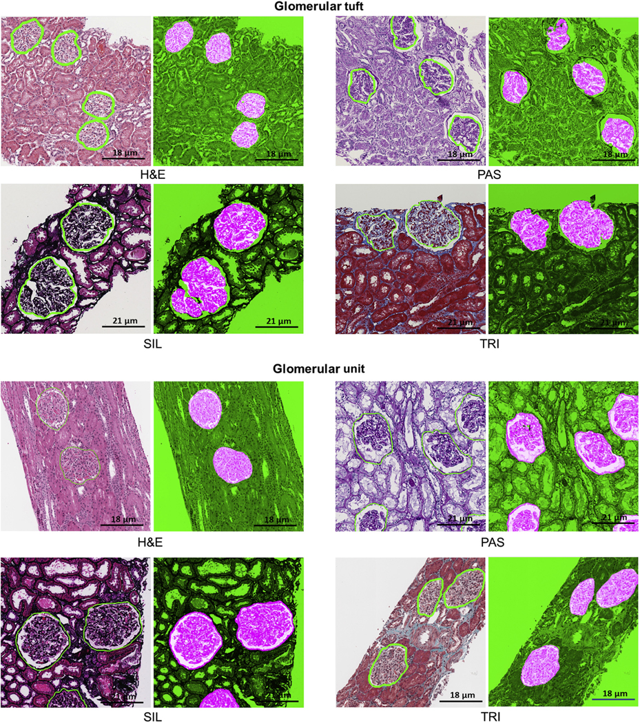
The classifier performed consistently across the 4 stains with only marginal differences in F-score and Dice similarity coefficient (DSC). A 5× digital magnification on PAS and H&E stains (Table 1, Figures 1 and 2) resulted in optimal detection and segmentation.

Table 1|.

Performance metrics: F, DSC, TPR, and PPV for structurally normal histologic primitives at optimal digital magnification

Stain		H&E				PAS				SIL				TRI
Histologic primitive	Optimal mag	F	DSC	TPR	PPV	F	DSC	TPR	PPV	F	DSC	TPR	PPV	F	DSC	TPR	PPV
Glomerular tuft	×5	0.91	0.93	0.89	0.93	0.96	0.97	0.94	0.93	0.90	0.96	0.91	0.87	0.89	0.94	0.91	0.89
Glomerular unit	×5	0.92	0.90	0.88	0.93	0.93	0.96	0.95	0.94	0.92	0.98	0.89	0.90	0.89	0.91	0.93	0.92
Proximal tubular segment	×10	0.89	0.95	0.93	0.84	0.91	0.90	0.98	0.92	0.90	0.88	0.96	0.90	0.90	0.89	0.97	0.91
Distal tubular segment	×10	0.78	0.78	0.83	0.80	0.93	0.92	0.96	0.93	0.91	0.93	0.89	0.90	0.81	0.82	0.80	0.84
Peritubular capillaries	×40	—	—	—	—	0.81	0.71	0.87	0.78	—	—	—	—	—	—	—	—
Arteries/arterioles	×10	0.83	0.85	0.84	0.83	0.85	0.90	0.93	0.82	—	—	—	—	0.79	0.86	0.89	0.86

F, F-score; DSC, dice similarity coefficient; H&E, hematoxylin and eosin; mag, magnification; PAS, periodic acid–Schiff; PPV, positive predictive rate; SIL, periodic acid–methenamine silver; TPR, true positive rate; TRI, Masson trichrome.

Figure 1|. Optimally digitally magnified regions of interest.

The optimal magnification varied for each histologic primitive using patch size of 256 × 256 px: periodic acid–Schiff glomerular unit and tuft, original magnification ×5; proximal and distal tubular segment, original magnification ×10; peritubular capillary, original magnification ×40; and arteries/arterioles, original magnification ×10 (not shown).

Figure 2|. Deep learning (DL) segmentation of glomerular tuft and unit.

DL segmentation for glomerular unit and tuft on whole slide images of formalin-fixed and paraffin-embedded sections from minimal change disease, stained with hematoxylin and eosin (H&E), periodic acid–Schiff (PAS), trichrome (TRI), and silver (SIL). For each stain, the original image overlaid with ground truth is presented on the left, and the DL segmentation is presented on the right. The positive classes are highlighted in bright pink from green transparent mask overlaid on original image. The DL output is specifically tracing the Bowman capsule for glomerular unit and the profile of the capillary wall for the glomerular tuft. The glomerular units and tufts were correctly identified across all types of stains.

Glomerular unit.

Consistent quantitative performance metric with F-score and DSC over 0.89 were observed across all stains, with optimal results for detection and segmentation using 5× digital magnification on PAS and SIL stains (Table 1, Figures 1 and 2).

Proximal tubular segments.

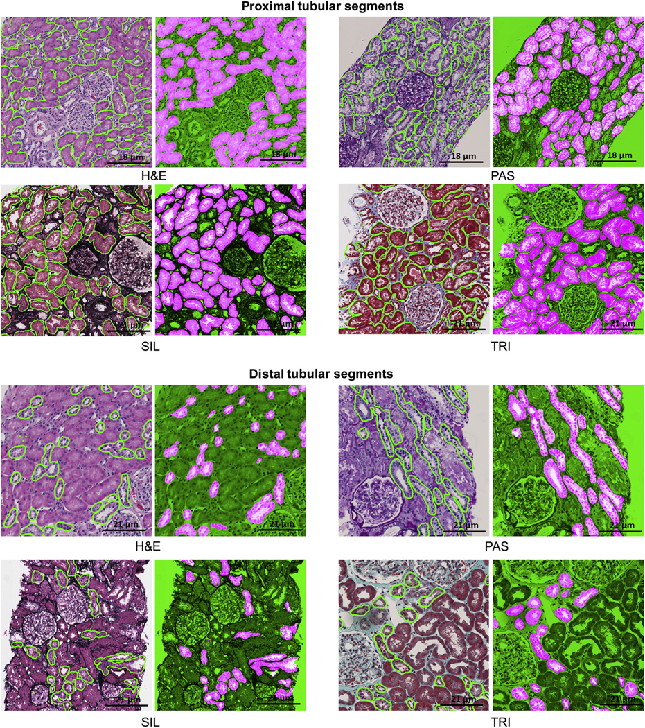
Segmentation results varied little across the stains (F-score from 0.89 to 0.91, and DSC from 0.88 to 0.95), with PAS, SIL, and TRI stains having better performance than the H&E stain. A 10× magnification was optimal for detection and segmentation across all stains. (Table 1, Figures 1 and 3).

Figure 3|. Deep learning (DL) segmentation of proximal and distal tubular segments.

DL segmentation for tubular segments on whole slide images of formalin-fixed and paraffin-embedded sections from minimal change disease, stained with hematoxylin and eosin (H&E), periodic acid–Schiff (PAS), trichrome (TRI), and silver (SIL). For each stain, the original image overlaid with ground truth is presented on the left, and the DL segmentation is presented on the right. The positive classes are highlighted in bright pink from green transparent mask overlaid on original image.

Distal tubular segments.

Segmentation results were highly variable across all the stains: F-scores were 0.78 and 0.81 for H&E and TRI, respectively, and 0.91 and 0.93 for SIL and PAS, respectively. DSC scores were 0.78 and 0.82 for H&E and TRI, and 0.92 and 0.93 for SIL and PAS. Optimal results for detection and segmentation were obtained using 10× digital magnification on PAS and SIL stains (Table 1, Figures 1 and 3).

Arteries/arterioles.

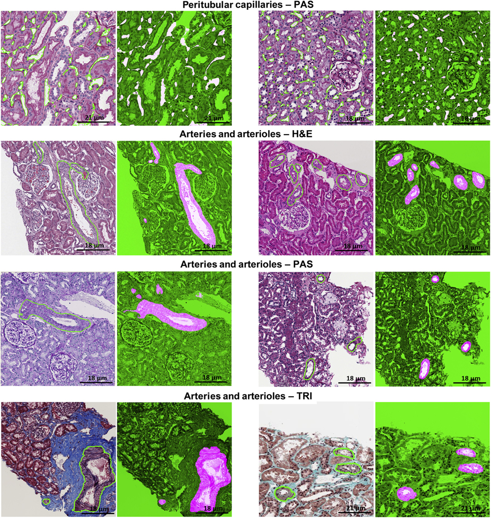
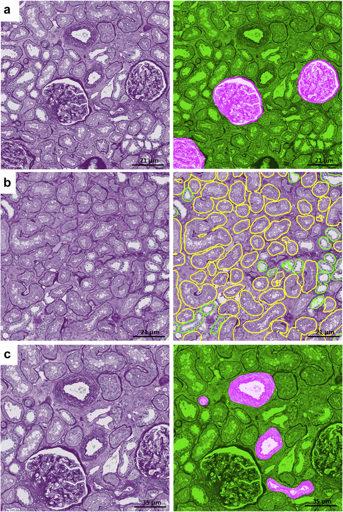
Artery/arteriole segmentation was variable across stains, with F-scores ranging from 0.79 to 0.85 across TRI, H&E, and PAS staining and DSC ranging from 0.85 to 0.90. Optimal results for detection and segmentation were obtained using 10× on PAS stain (Table 1, Figures 1 and 4).

Figure 4|. Deep learning (DL) segmentation of arteries/arterioles and peritubular capillaries.

DL segmentation for arteries/arterioles on whole slide images of formalin-fixed and paraffin-embedded sections from minimal change disease, stained hematoxylin and eosin (H&E), periodic acid–Schiff (PAS), trichrome (TRI), and silver (SIL), and for peritubular capillaries on whole slide images of formalin-fixed and paraffin-embedded sections stained with PAS, with the original image overlaid with ground truth on the left and the DL segmentation on the right. The positive classes are highlighted in bright pink from green transparent mask overlaid on original image.

Peritubular capillaries.

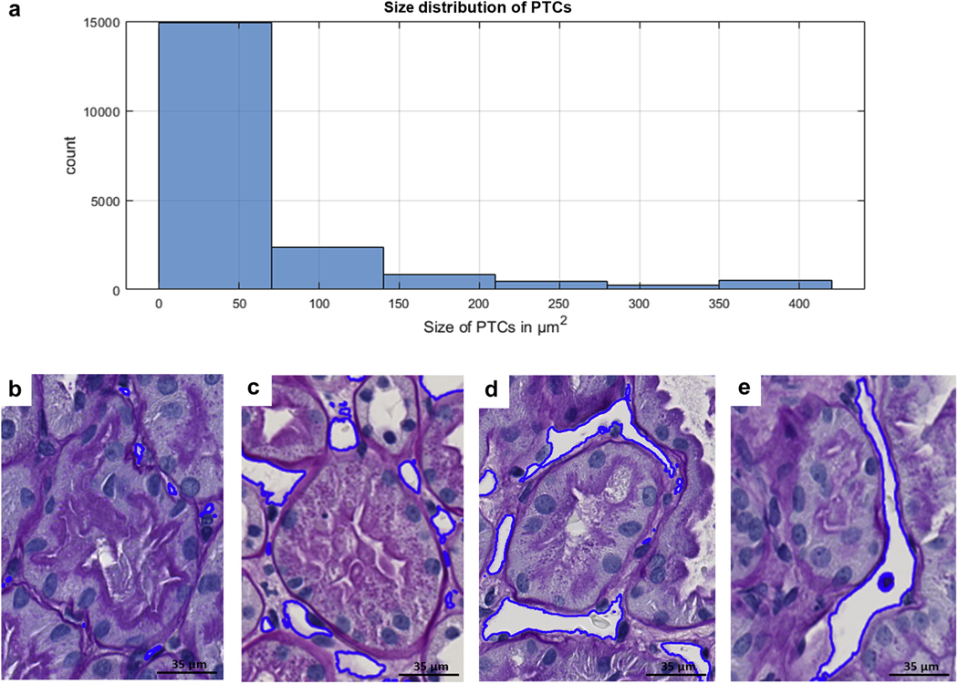
Optimal results for detection and segmentation were obtained using 40× magnification on PAS stain (Table 1, Figures 1 and 4). Qualitative segmentation results on the testing cohort show that most of the large-sized peritubular capillaries were thin and long as they were cut tangentially from the biopsy. Although the size, shape, and textural presentation of peritubular capillaries varied (Figure 5a), the U-Net model was able to detect and segment peritubular capillaries of varying sizes and shapes (Figure 5). The classifier tends to perform better on thin and long, small- to medium-sized capillaries. However, capillaries with size less than 40 pixels (167 μm²) failed to be identified or were inaccurately segmented.

Figure 5|. Deep learning (DL) Segmentation performance in relation to the morphologic heterogeneity of peritubular capillaries (PTCs).

(a) Most of the peritubular capillaries were small when measured in number of pixels. The size of the peritubular capillaries has an exponential distribution with a long tail from small to large. Each pixel is 0.06 μm2 on tissue, and as observed, most of the PTCs are under 90 μm2. Examples of DL performance on small (c), medium (b), and large (d,e) PCs.

Validation of DL models using nephrectomies.

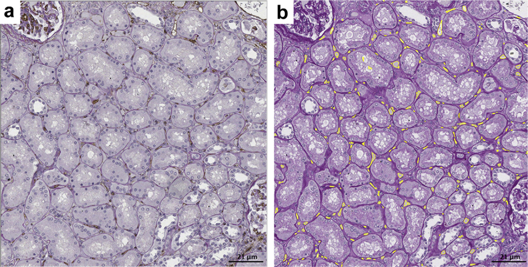
An F-score of 0.93 was obtained for 191 glomerular units, 0.90 for 1484 proximal tubules, 0.93 for 1251 distal tubules, 0.71 for 269 arteries/arterioles (Figure 6), and 0.90 for 3784 peritubular capillaries (Figure 7). The rare globally sclerotic glomeruli and atrophic tubules present in the sections were not segmented by the DL network.

Figure 6|. Deep learning (DL) segmentation of normal histologic primitives on periodic acid–Schiff nephrectomies.

(a) Segmentation of normal glomerular units. (b) Segmentation of proximal (yellow) and distal (green) tubules; rare atrophic tubules were detected by the DL algorithms. (c) Segmentation of arteries/arterioles.

Figure 7|. Segmentation outputs of peritubular capillaries (PTCs) on periodic acid–Schiff (PAS) nephrectomies.

(a) Formalin-fixed and paraffin-embedded sections stained with PAS and CD34 (double stain). (b) Deep learning (DL) segmentation of peritubular capillaries on the same section stained with PAS alone. There is overlap between the CD34 positive stain and the DL detection of peritubular capillaries. Overall, the DL performance was similar to the segmentation accuracy on the testing set for minimal change disease.

DL segmentation performance across sites and artifacts.

See Supplementary Figure S4.

DL performance as a function of number of training exemplars

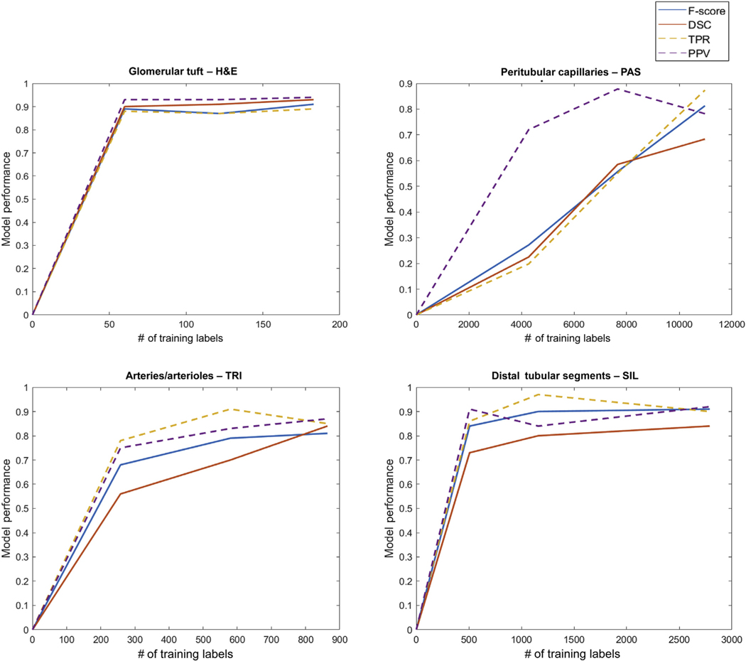
The rate of improvement of the network performance as a function of the number of training exemplars was observed to be different across histologic primitives. The number of exemplars needed to maximize network performance increases substantially from glomerular tufts to distal tubular segments, arteries/arterioles, and finally to peritubular capillaries (Figure 8). For larger structures such as glomerular tufts, it was observed that only 60 training samples were necessary to achieve an F-score of 0.89, with a 0.02 increase using 183 tufts. For smaller and largely represented structures such as distal tubules, a 0.07 increase in F-score was observed by increasing the number of exemplars from 507 to 2789. For structures such as arteries/arterioles with varying sizes, the F-score increased by 0.13, increasing the number of exemplars from 258 to 864. A significant increase in F-score from 0.27 to 0.81 was observed with peritubular capillaries by increasing the number of exemplars 2.5 times (i.e., from 4273 to 10,975).

Figure 8|. Model performance with increasing number of training annotations.

Number of annotations versus deep learning model performans. The model performance was measured as F-score, dice similarity coefficient (DSC), true positive rate (TPR), predictive positive value (PPV). For histologic primitives such as glomerular tufts, only a small number of annotations was required to construct a robust classifier, in contrast to peritubular capillaries where larger number of annotations were required. The performance metrics for peritubular capillary segmentation increased linearly as more annotations were added. Arteries/arterioles and distal tubules had intermediate rates of convergence with increasing number of annotations.

DISCUSSION

The assessment of renal biopsy is unique compared with other surgical pathology specimens because of the variety of stains routinely used. Morphologic assessment relies on the quality of the preparations, the pathologists’ expertise in detecting the individual structures and associated changes, and quantitative or semiquantitative metrics used to capture the extent of tissue damage. Visual histologic quantitative assessment such as counting, distribution, and morphometry of certain histologic primitives are known to be robust predictors of outcome for various kidney diseases.^10,17–23 However, quantitative analysis remains a challenge for the human eye. Some of these primitives (e.g., peritubular capillaries) cannot be measured visually or manually and warrant the aid of computational algorithms. Recent studies have suggested that computer vision tools can serve as triage and decision support tools for disease diagnosis with digital pathology.^24–27 Thus, automated image analysis tools need to be implemented and integrated into the pathology workflow for efficient and reliable segmentation of histologic primitives across multiple types of stains. DL segmentation tools could greatly facilitate derivation of not only the visual but also subvisual histomorphometric features (e.g., shape, textural, and graph features) for correlation with diagnosis and outcome.^28–30

This study attempts to address the challenges of computational renal pathology for large-scale tissue interrogation by providing DL algorithms for thorough annotation of 6 histologic primitives on renal parenchyma of minimal change disease (MCD), using whole slide images (WSIs) of 4 stains and generated across 29 NEPTUNE enrolling centers. In the past few years, several studies have demonstrated the utility of DL networks for low-level image analyses (i.e., detection, segmentation, and classification of histologic primitives) and high-level complex prognosis and prediction tasks.^31–35 Our study is the largest, comprehensive DL study of kidney biopsies, presenting algorithms that were developed on different stains and using a large number of annotated images, compared with those previously published. The primary conclusions and significant findings from our work are described next.

Comparison with current literature

The differences between previous studies^36–44 and our contributions are summarized in the Supplementary Figure S6. Previously published studies focus on a single histologic primitive and a single stain. For example, Marsh et al. evaluated CNNs for detection of global glomerulosclerosis in transplant kidney frozen sections stained with H&E³⁶; Kanna et al. evaluated CNNs to discriminate normal, segmentally and globally sclerosed glomeruli from trichrome stained formalin-fixed and paraffin-embedded kidney sections³⁷; Gallego et al. applied DL to detect glomeruli on PAS-stained sections; Bel et al. demonstrated segmentation of normal and pathologic histologic structures using PAS stained WSIs of nephrectomy cortex tissue.³⁹ Temerinac-Ott et al. demonstrate a DL approach to improve glomerular detection on 1 staining using results from differently stained sections of same tissue.³⁸ Our DL networks on all 4 stains represent a first step for future clinical deployment allowing for the detection, segmentation, and ultimately quantification of several normal histologic primitives in all stains routinely used for diagnostic purposes.

Another critical element that needs to be taken into consideration before their use in large-scale DL networks is how they can be applied to heterogeneous datasets. Our DL models were trained and tested on a very heterogeneous set of WSIs with preanalytic variations in tissue acquisition, processing, and slide preparation using 4 stains, thus facilitating the rigorous evaluation of the applicability of the DL approach in a multisite setting.

Different DL approaches have been used for the segmentation of histologic primitives, such as Gadermayr et al.’s application of generative adversarial deep networks for stain-independent glomerular segmentation.⁴⁵ Bel et al. employed cycle-consistent generative adversarial networks (cycle-GANs) in DL applications for multicenter stain transformation.⁴⁰ Hermsen et al. has demonstrated U-Net based segmentation of 7 tissue classes using 40 transplant biopsies on PAS stain.⁴² Our approach, in this study, was to develop multiple U-Net based DL networks using optimal digital magnification and varying number of annotations across primitives and stains.

All previous works have used relatively smaller number of WSIs of renal biopsies/nephrectomies compared with our study (Table 2). The use of a large WSI dataset allowed us to provide insights to pathologists for generating well-annotated training exemplars for each primitive and stain, as well as the number of training exemplars required for best network performance using U-Net CNNs (Figure 8).

Table 2|.

DL dataset showing the number of training and testing region of interest images extracted from 459 WSIs of 125 MCD patients and the number of manually segmented annotations for 6 structurally normal histologic primitives

Histologic primitive for DL segmentation	Stain	No. of manual segmentations	No. of images (3000 × 3000 px) extracted from the WSIs
Glomeruli	H&E	240	Gt 150, Gu 150
	PAS	373	Gt 228, Gu 204
	SIL	267	Gt-124, Gu-124
	TRI	316	Gt-138, Gu 137
Proximal tubular segments	H&E	1329	108
	PAS	1621	66
	SIL	891	102
	TRI	828	94
Distal tubular segments	H&E	595	108
	PAS	816	66
	SIL	509	102
	TRI	365	94
Peritubular capillaries	PAS	19,280	121
Arteries/arterioles	H&E	1153	344
	PAS	508	238
	TRI	957	422

DL, deep learning; Gt, glomerular tuft; Gu, glomerular unit (tuft + Bowman capsule); H&E, hematoxylin and eosin; mag, magnification; MCD, minimal change disease; PAS, periodic acid–Schiff; SIL, periodic acid–methenamine silver; TRI, Masson trichrome; WSI, whole slide images.

Specificity of the segmentation of the individual histologic primitives and their pathologic variation is critical for the deployment of DL models into clinical practice.^42,43 The DL networks generated in this work are specific to structurally normal histologic primitives, such as those seen in MCD or nephrectomies, and can be applied to both adult and pediatric renal biopsies. When the DL networks were tested on patches of renal parenchyma from nephrectomy specimens, the specificity for the structurally normal histologic primitives was maintained. The DL framework presented in this study will also enable architecting of networks in the future that are specifically focused on automated segmentation and assessment of structurally abnormal histologic primitives and their correlation with clinical outcomes.

DL-based ranking of different stains

Our study suggests that the PAS stain is best suited for identification of structurally normal histologic primitives using the U-Net model. This may be because PAS appears to be consistently more homogeneous across pathology laboratories compared with TRI or SIL. PAS-stained WSIs highlight the basement membranes of different structures, which in turn provides superior definition of the boundary of each single primitive to be segmented. For this reason, PAS was the only stain used for segmentation of peritubular capillaries. On the basis of our results, PAS and H&E stains showed better performance for glomerular tuft and unit segmentation, PAS and TRI for arteries/arterioles, PAS and SIL for tubular segments, and PAS for peritubular capillaries.

Optimal digital magnification for DL models

Our results suggest that with a unified patch size of 256 × 256, optimal magnification for the DL models was 5× for glomeruli, 10× for tubules and vessels, and 40× for capillaries (Figure 1). Interestingly, most of the optimal magnifications were concordant with the magnifications that pathologists tend to use when annotating the individual primitives, except for glomeruli where the pathologists used 15× to 20×. Larger structures such as glomeruli, tubules, and vessels were more precisely segmented by the network at 5× to 10× magnification regardless of the stain. For smaller structures such as peritubular capillaries, larger digital magnification (40×) was required for accurate DL segmentation.

DL segmentation performance across sites and artifacts

Heterogeneity of tissue preparation and lack of standardization of the analytics is particularly relevant for multicenter studies, where the pathology material is collected from several laboratories. As expected, heterogeneity in tissue presentation and glass, tissue, and scanning artifacts was observed, each with variable contribution to the DL performance. For example, although in general tissue artifacts had limited impact on the DL networks, the thickness of the section appeared to affect performance. The impact of individual artifacts was also relative to the histologic primitive; for example, glass artifacts showed a slight negative impact on DL performance for arteries/arterioles and proximal tubules. Additionally, there was variability in DL performance across sites, and this variability appeared to be histologic primitive dependent (Supplementary Figure S4).

DL performance as a function of number of training exemplars

Our quantitative data validated the intuitive assumption that more exemplars are needed for those primitives that are more difficult to identify visually (i.e., tangentially cut arteries/arterioles or primitives at the edge of the region of interest [ROI]) (Figure 8). For those primitives that were too small or ill defined (i.e. peritubular capillaries), curation and iterative annotation was necessary to improve segmentation accuracy. For segmentation of glomerular tufts, the network converged to maximum accuracy with a small number (60–183) of training exemplars; performance did not improve with inclusion of additional exemplars. For tubules and arteries/arterioles segmentation, the corresponding networks showed marginal to intermediate performance improvement with an increasing number of exemplars. In contrast, a significant increase in F-score and DSC (0.27–0.81) was observed with a 2.5-fold increase in the number of peritubular capillary exemplars, a linear scope of F-score increase indicating even better accuracy with more exemplars.

Interpreting segmentation results

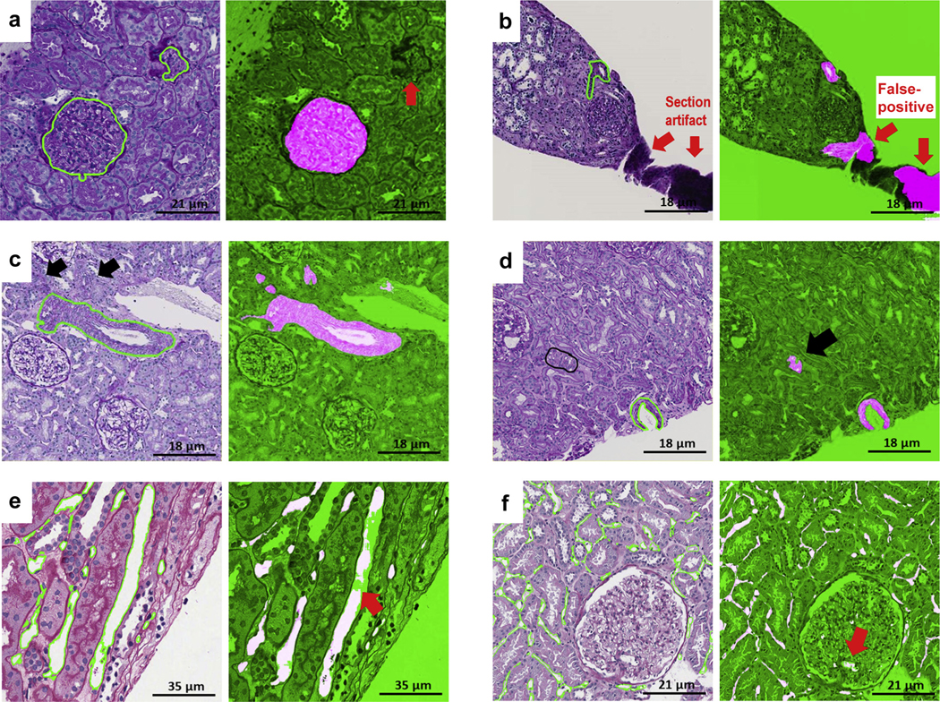
Few false positives were observed in regions of interest with artifacts (i.e. tissue folds, uneven staining), suggesting the need for digital quality assessment of the slide images prior to invocation of the computational models (Supplementary Figure S4). In a few ROIs, the DL appeared to outperform the pathologists—for example, when a small portion of an artery/arteriole was at the edge of the ROIs and was not manually annotated as ground truth by the pathologist because they were visually difficult to detect. This can be explained by the protocol used for segmentation of arteries, where pathologists included only arteries where the wall (tunica media and intima) and lumen were visible and segmented the outer boundary of the tunica media. Thus, the models, trained to detect the tunica media and intima of the arteries correctly identified small fragments of tunica media (arterial/arteriolar wall tangentially cut) as arteries/arterioles despite the lack of a lumen (Figure 9).

Figure 9|. Examples of false positive and false negative deep learning (DL) segmentations on periodic acid–Schiff (PAS).

(a) Glomerular unit: DL failed to detect a tangentially cut glomerular unit that does not have a typical round shape (red thick arrow). (b) Artery: section artifact generate a false positive (red thick arrows). (c) Arteries: black arrows show 2 arterioles missed by the pathologist but detected by DL. (d) Arteries: pathologists were instructed to segment artery when lumen was present; however, DL segmentation detected tangentially cut artery (thick black arrow) where only the medium was visible. (e) Peritubular capillaries: a long peritubular capillary reveals only partial DL segmentation at the pixel level. (f) Peritubular capillaries: DL network for peritubular capillaries detects a few glomerular capillaries (false positive; thick red arrow).

Additionally, tubules in renal biopsy sections are more often seen in transverse than longitudinal sections. The initial classifier missed some longitudinally sectioned tubules, mostly on H&E-stained images, because the tubule boundaries were less sharp, and longitudinally sectioned tubules were underrepresented in the initial training set. To facilitate and improve the process of annotation and the network, the false-negative errors associated with the U-Net segmentation of the tubules were visually identified and manually refined by the pathologist, and the updated annotations were returned to the network. A few small arterioles were also incorrectly identified as distal tubules by the DL algorithm (false positives) during the first iteration. These false-positive annotations were removed by the pathologist upon review of the initial classifier output and corrected images were returned to the network for retraining without changing the experimental setup or the network parameters to eliminate false positives and negative errors of the DL algorithm.⁴⁵

In line with current sharing guidelines, with this report, we are making all of our data and accompanying ground truth annotations publicly available for the community. Online supplemental material released as part of this work is anticipated to advance the field of computational renal pathology⁴⁶ and provide best practices for generating annotations, augmentations,⁴⁷ magnifications and recommended stains to perform segmentation tasks optimally.

In conclusion, this study represents a solid foundation toward invoking machine learning classifiers to aid large-scale tissue quantification efforts and the implementation of machine–human interactive protocols in clinical and pathology workflows. DL segmentation of histologic primitives enables computational derivation of histomorphometric features for enabling biopsy interpretation. Additionally, the framework presented in this work will also pave the way for development of new DL networks in the future that are specifically geared toward (i) abnormal or pathologic histologic primitives (i.e., global and segmental sclerosis, glomerular proliferative features, collecting ducts, veins and peripheral nerves, tubular atrophy, interstitial fibrosis, and arteriosclerosis), (ii) renal cortex and medullary compartments, and (iii) a wider spectrum of diseases. Further, these novel approaches could pave the way for the development of machine learning tools that provide disease prognosis or predicting treatment response²⁴ and even facilitate discovery of clinically actionable, nondestructive computational pathology–based imaging diagnostic biomarkers for kidney diseases.^25,27,48

METHODS

Case and image dataset selection

This study was conducted using digital renal biopsies from the NEPTUNE digital pathology repository. NEPTUNE is a North American multicenter collaborative consortium with more than 650 adult and children enrolled from 29 recruiting sites (38 pathology laboratories). Only cases with a diagnosis of MCD were included in this study because histologically they are the most similar to normal renal parenchyma. A total of 459 curated WSIs (125 H&E, 125 PAS, 102 SIL, 107 TRI) from 125 MCD renal biopsies were used.⁴⁹ Not all cases had all stains available in the digital pathology repository. Four WSIs were selected for each patient (1 WSI per stain). From each WSI, approximately 3 to 5 ROIs containing the histologic primitives were randomly selected, inspected by a pathologist, and manually extracted as 3000 × 3000 tiles then stored as 8-bit red-green-blue (RGB) color images in PNG format at 40× digital magnification. Additional details on digitization and curation of biopsy WSIs can be found in Supplementary Figure S1.

Independent validation of the DL models.

Six WSIs from 3 formalin-fixed and paraffin-embedded nephrectomy specimens were included to test the DL network performance for the segmentation of all histologic primitives on adult renal parenchyma without significant structural abnormalities. Sections from the nephrectomy specimens were stained with PAS, scanned into WSIs, and subsequently stained with a CD34 antibody, a marker of endothelial cells, and then rescanned into WSIs. One hundred seventy-five random ROIs (3000 × 3000 pixels) were extracted from the PAS-stained WSIs. The PAS-CD34 double-stained WSIs were used as ground truth for validation of the DL segmentation approach for peritubular capillaries.

Histologic primitives and manual segmentation

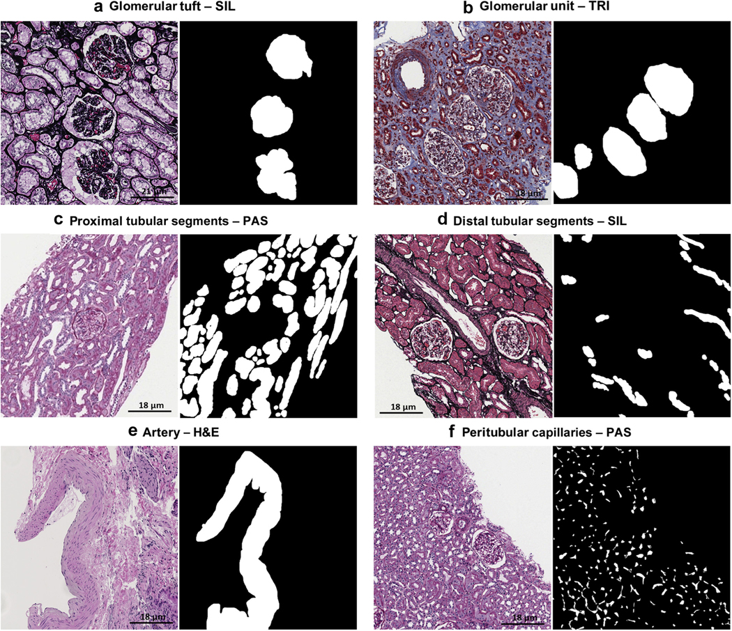
Five renal pathologists manually segmented the ROIs to establish the ground truth for the histologic primitives (Table 2). Manual segmentations were generated using an open-source software application.¹⁵ The ground truth annotations were saved as binary masks; that is, each pixel that was denoted as part of a histologic primitive (positive class pixels expressed as binary 1s) or not (negative class pixels expressed as binary 0s). Through this process, 30,048 annotations were made by pathologists on 1818 ROIs (Figure 10).

Figure 10|. Ground truth annotation for histologic primitives.

Examples of manual annotation on histologic primitives on whole slide images of formalin-fixed and paraffin-embedded sections from minimal change disease, stained with hematoxylin and eosin (H&E), periodic acid–Schiff (PAS), trichrome (TRI), and silver (SIL), and corresponding binary masks (black and white pictures) are shown.

Six histologic primitives were used for this study: glomerular tuft, glomerular unit (tuft + Bowman’s capsule), proximal tubular segments, distal tubular segments, arteries and arterioles, and peritubular capillaries. Consistent and detailed ground truth labels across all training samples can greatly facilitate robust DL performance, especially in segmentation tasks.^{24,32,36,50–54} In order to produce consistent annotations across all images, each histologic primitive and its boundaries were carefully defined, and the annotation procedure for each use case standardized (Supplementary Figure S2). Furthermore, each annotation generated by a pathologist was reviewed by a second pathologist for quality assessment.

DL experimental pipeline and training methods

DL dataset.

Up to four WSIs per biopsy (H&E, PAS, TRI, and SIL for each) were used for the segmentation of the glomerular tuft and unit, and proximal and distal tubular segments. Peritubular capillaries were segmented using only PAS WSIs, and arteries/arterioles were segmented only in H&E, PAS, and TRI WSIs (Table 2). WSIs were divided at the patient level into training, validation, and testing sets (ratio 6:1:3). The networks were developed using WSIs of both adult and pediatric patients (Supplementary Figure S1). For training of the U-Net network, 5 pathologists annotated 1196 glomerular tufts and units, 4669 proximal and 2285 distal tubular segments, 19,280 peritubular capillaries, and 2261 arteries/arterioles (Table 2).

Network configuration and training.

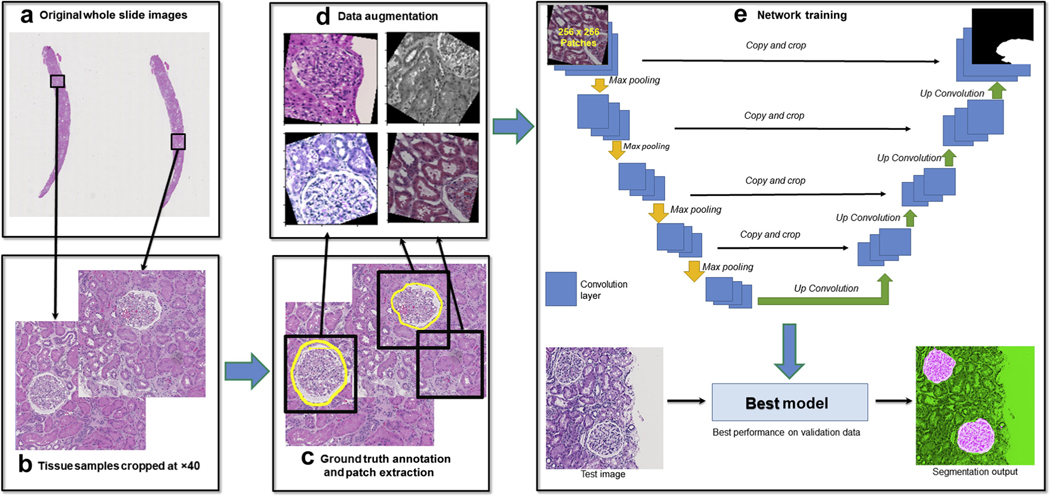
Standard U-Net architecture with slightly tweaked parameters were implemented in PyTorch framework for training of each use case (Figure 11). Details of U-Net configuration, training methods including training set balancing and data augmentation can be found in Supplemental S3.

Figure 11|. Flowchart of the workflow of deep learning (DL) experimental pipeline for each stain and use case.

(a) Whole slide images (WSIs) were selected for generation of training, validation, and testing data. (b) Regions of interest were cropped from original WSIs with 40× digital magnification. (c) Ground truth labels were generated by pathologists for training, and overlapping patches of size 256 × 256 px (0.24 μm/px) containing both image data and ground truth annotation information were cropped from the training and validation images (as shown in black boxes). (d) For each path, a randomized data augmentation method is introduced to account for (i) size variation of primitives, (ii) stain variations, and (iii) tissue variations (e.g. thickness). (e) All the training patches were passed to U-Net on PyTorch for training, and validation patches were used to generate loss and accuracy measures for each epoch trained to evaluate model performance. Finally, the epoch that yielded the lowest loss on the validation data was selected for generation of test results.

Detection and segmentation metrics.

Detection and segmentation results were evaluated using F-Score, true positive rate (TPR), positive predictive value (PPV), and DSC.^55–57 Values of 0 and 1 represent the maximal discordance and agreement, respectively, between the pathologist ground truth and the U-Net results. TPR, PPV, and F-Score measure the detection accuracy of the DL networks. These metrics are computed using the number of correct segmentation results (true positives), incorrect segmentations (false positives), and missing segmentations (false negatives). DSC is the pixel-wise spatial overlap index that measures the segmentation accuracy of the classifier, with values ranging from 0 (indicating no spatial overlap between ground truth annotation and corresponding DL output mask) to 1 (indicating complete overlap), and a DSC value >0.5 denoting a correct segmentation (true positive).

Number of training exemplars for different histologic primitives

To test how the number of manually annotated training exemplars influences network performance, we selected a representative set of histologic primitives based on size, complexity, distribution, and stain: glomerular tufts on H&E, peritubular capillaries on PAS, distal tubular segments on TRI, and arteries/arterioles on SIL. Specifically, we sought to evaluate the minimum number of annotated exemplars for standing up trained U-Net models for each type of histologic primitive. Toward this end, multiple U-Net models were trained for each type of primitive, each time with a greater number of annotated exemplars. Detection and segmentation accuracy were then computed for each such U-Net model for each primitive on the corresponding testing sets (Figure 8).

DL segmentation performance across sites and artifacts

See Supplementary Figure S4.

Supplementary Material

Supplementary Material

Figure S1.Digitization and curation of renal biopsy whole slide images.

Figure S2.Histologic primitives and criteria for segmentation.

Figure S3.Network training, data augmentation, balanced sampling and pre- and post-processing.

Translational Statement.

The assessment of renal biopsy is unique compared with other surgical pathology specimens because of the variety of stains routinely used. Morphologic assessment of histological preparations relies on the quality of the preparations itself, as well as the expertise of the pathologist in identifying normal and pathological structures. The authors demonstrate that “deep learning–based convolutional neural networks” may be employed for efficient and reliable segmentation of histologic structures across different stains of normal renal parenchyma using the Nephrotic Syndrome Study Network whole slide images. This dataset was curated from 38 histology laboratories and reflects substantial morphologic, technical, and stain heterogeneity. The findings provide useful insights, along with source code and data, which will help readers overcome challenges in this space. Taken together, this work represents a technical foundation from which future pathology tools may be built to enable actionable clinical decision support tools for better disease characterization and risk assessment in pathology workflows.

APPENDIX

Members of the Nephrotic Syndrome Study Network (NEPTUNE)

NEPTUNE Enrolling Centers.

Cleveland Clinic, Cleveland, OH: J. Sedor*, K. Dell*, M. Schachere^#, J. Negrey^#

Children’s Hospital, Los Angeles, CA: K. Lemley*, E. Lim^#

Children’s Mercy Hospital, Kansas City, MO: T. Srivastava*, A. Garrett^#

Cohen Children’s Hospital, New Hyde Park, NY: C. Sethna*, K. Laurent^#

Columbia University, New York, NY: G. Appel*, M. Toledo^#

Duke University, Durham, NC: L. Barisoni*

Emory University, Atlanta, GA: L. Greenbaum*, C. Wang**, C. Kang^#

Harbor-University of California Los Angeles Medical Center: S. Adler*, C. Nast*^‡, J. LaPage^#

John H. Stroger Jr. Hospital of Cook County, Chicago, IL: A. Athavale*, M. Itteera

Johns Hopkins Medicine, Baltimore, MD: A. Neu*, S. Boynton^#

Mayo Clinic, Rochester, MN: F. Fervenza*, M. Hogan**, J. Lieske*, V. Chernitskiy^#

Montefiore Medical Center, Bronx, NY: F. Kaskel*, N. Kumar*, P. Flynn^# NIDDK Intramural, Bethesda, MD: J. Kopp*, J. Blake^#

New York University Medical Center, New York, NY: H. Trachtman*, O. Zhdanova**, F. Modersitzki^#, S. Vento^#

Stanford University, Stanford, CA: R. Lafayette*, K. Mehta^#

Temple University, Philadelphia, PA: C. Gadegbeku*, D. Johnstone**, S. Quinn-Boyle^#

University Health Network Toronto: D. Cattran*, M. Hladunewich**, H. Reich**, P. Ling^#, M. Romano^#

University of Miami, Miami, FL: A. Fornoni*, C. Bidot^#

University of Michigan, Ann Arbor, MI: M. Kretzler*, D. Gipson*, A. Williams^#, J. LaVigne^#

University of North Carolina, Chapel Hill, NC: V. Derebail*, K. Gibson*, A. Froment^#, S. Grubbs^#

University of Pennsylvania, Philadelphia, PA: L. Holzman*, K. Meyers**, K. Kallem^#, J. Lalli^#

University of Texas Southwestern, Dallas, TX: K. Sambandam*, Z. Wang^#, M. Rogers^#

University of Washington, Seattle, WA: A. Jefferson*, S. Hingorani**, K. Tuttle**^x, M. Bray^#, M. Kelton^#, A. Cooper^#§

Wake Forest University Baptist Health, Winston-Salem, NC: B. Freedman*, J.J. Lin**

Data Analysis and Coordinating Center.

M. Kretzler, L. Barisoni, C. Gadegbeku, B. Gillespie, D. Gipson, L. Holzman, L. Mariani, M. Sampson, J. Troost, J. Zee, E. Herreshoff, S. Li, C. Lienczewski, J. Liu, T. Mainieri, M. Wladkowski, and A. Williams.

Digital Pathology Committee.

Carmen Avila-Casado (UHN-Toronto), Serena Bagnasco (Johns Hopkins), Joseph Gaut (Washington U), Stephen Hewitt (National Cancer Institute), Jeff Hodgin (University of Michigan), Kevin Lemley (Children’s Hospital LA), Laura Mariani (University of Michigan), Matthew Palmer (U Pennsylvania), Avi Rosenberg (NIDDK), Virginie Royal (Montreal), David Thomas (University of Miami), Jarcy Zee (Arbor Research). Co-Chairs: Laura Barisoni (Duke University) and Cynthia Nast (Cedar Sinai).

*Principal investigator; **co-investigator; ^#study coordinator

^‡Cedars-Sinai Medical Center, Los Angeles, CA

^§Providence Medical Research Center, Spokane, WA

REFERENCES

- 1.Hill NR, Fatoba ST, Oke JL, et al. Global prevalence of chronic kidney disease—a systematic review and meta-analysis. PLoS ONE. 2016;11: e0158765. [DOI] [PMC free article] [PubMed] [Google Scholar]
- 2.Bandari J, Fuller TW, Ii RMT, D’Agostino LA. Renal biopsy for medical renal disease: indications and contraindications. Can J Urol. 2016;23: 8121–8126. [PubMed] [Google Scholar]
- 3.Hogan JJ, Mocanu M, Berns JS. the native kidney biopsy: update and evidence for best practice. Clin J Am Soc Nephrol. 2016;11:354–362. [DOI] [PMC free article] [PubMed] [Google Scholar]
- 4.Barisoni L, Gimpel C, Kain R, et al. Digital pathology imaging as a novel platform for standardization and globalization of quantitative nephropathology. Clin Kidney J. 2017;10:176–187. [DOI] [PMC free article] [PubMed] [Google Scholar]
- 5.Oni L, Beresford MW, Witte D, et al. Inter-observer variability of the histological classification of lupus glomerulonephritis in children. Lupus. 2017;26:1205–1211. [DOI] [PubMed] [Google Scholar]
- 6.Wernick RM. Reliability of histologic scoring for lupus nephritis: a community-based evaluation. Ann Intern Med. 1993;119:805–811. [DOI] [PubMed] [Google Scholar]
- 7.Barisoni L, Troost JP, Nast C, et al. Reproducibility of the NEPTUNE descriptor-based scoring system on whole-slide images and histologic and ultrastructural digital images. Mod Pathol. 2016;29:671–684. [DOI] [PMC free article] [PubMed] [Google Scholar]
- 8.Barisoni L, Hodgin JB. Digital pathology in nephrology clinical trials, research, and pathology practice. Curr Opin Nephrol Hypertens. 2017;26: 450–459. [DOI] [PMC free article] [PubMed] [Google Scholar]
- 9.Barisoni L, Nast CC, Jennette JC, et al. Digital pathology evaluation in the multicenter Nephrotic Syndrome Study Network (NEPTUNE). Clin J Am Soc Nephrol CJASN. 2013;8:1449–1459. [DOI] [PMC free article] [PubMed] [Google Scholar]
- 10.Mariani LH, Martini S, Barisoni L, et al. Interstitial fibrosis scored on whole-slide digital imaging of kidney biopsies is a predictor of outcome in proteinuric glomerulopathies. Nephrol Dial Transplant. 2018;33:310–318. [DOI] [PMC free article] [PubMed] [Google Scholar]
- 11.Recommended special stains/IHC for kidney biopsies. Available at: http://www.pathologyoutlines.com/topic/kidneyspecialstainsforbiopsies.html.Accessed September 11, 2019.
- 12.Venkatesh V, Malaichamy V. Role of special stains as a useful complementary tool in the diagnosis of renal diseases: a case series study. Int J Res Med Sci. 2019;7:1539. [Google Scholar]
- 13.Ronneberger O, Fischer P, Brox T. U-Net: Convolutional networks for biomedical image segmentation. ArXiv:1505:04597 [Cs] [e-pub ahead of print]. May 2015. Available at: http://arxiv.org/abs/1505.04597. Accessed June 13, 2019. [Google Scholar]
- 14.Janowczyk A, Madabhushi A. Deep learning for digital pathology image analysis: a comprehensive tutorial with selected use cases. J Pathol Inform. 2016;7:29. [DOI] [PMC free article] [PubMed] [Google Scholar]
- 15.Madabhushi A, Lee G. Image analysis and machine learning in digital pathology: challenges and opportunities. Med Image Anal. 2016;33:170–175. [DOI] [PMC free article] [PubMed] [Google Scholar]
- 16.Litjens G, Kooi T, Bejnordi BE, et al. A survey on deep learning in medical image analysis. Med Image Anal. 2017;42:60–88. [DOI] [PubMed] [Google Scholar]
- 17.Haruhara K, Tsuboi N, Sasaki T, et al. Volume ratio of glomerular tufts to Bowman capsules and renal outcomes in nephrosclerosis. Am J Hypertens. 2019;32:45–53. [DOI] [PubMed] [Google Scholar]
- 18.Lemley KV, Bagnasco SM, Nast CC, et al. Morphometry predicts early GFR change in primary proteinuric glomerulopathies: a longitudinal cohort study using generalized estimating equations. PLoS ONE. 2016;11: e0157148. [DOI] [PMC free article] [PubMed] [Google Scholar]
- 19.Srivastava A, Palsson R, Kaze AD, et al. The prognostic value of histopathologic lesions in native kidney biopsy specimens: results from the Boston Kidney Biopsy Cohort Study. J Am Soc Nephrol. 2018;29:2213–2224. [DOI] [PMC free article] [PubMed] [Google Scholar]
- 20.Kopp JB. Global glomerulosclerosis in primary nephrotic syndrome: including age as a variable to predict renal outcomes. Kidney Int. 2018;93: 1043–1044. [DOI] [PubMed] [Google Scholar]
- 21.Howie AJ, Ferreira MA, Adu D. Prognostic value of simple measurement of chronic damage in renal biopsy specimens. Nephrol Dial Transplant. 2001;16:1163–1169. [DOI] [PubMed] [Google Scholar]
- 22.Hommos MS, Zeng C, Liu Z, et al. Global glomerulosclerosis with nephrotic syndrome; the clinical importance of age adjustment. Kidney Int. 2018;93:1175–1182. [DOI] [PMC free article] [PubMed] [Google Scholar]
- 23.Venkatareddy M, Wang S, Yang Y, et al. Estimating podocyte number and density using a single histologic section. J Am Soc Nephrol. 2014;25: 1118–1129. [DOI] [PMC free article] [PubMed] [Google Scholar]
- 24.Bera K, Schalper KA, Rimm DL, et al. Artificial intelligence in digital pathology—new tools for diagnosis and precision oncology. Nat Rev Clin Oncol. 2019;16:703–715. [DOI] [PMC free article] [PubMed] [Google Scholar]
- 25.Becker JU, Mayerich D, Padmanabhan M, et al. Artificial intelligence and machine learning in nephropathology. Kidney Int. 2020;98:65–75. [DOI] [PMC free article] [PubMed] [Google Scholar]
- 26.Shin H, Roth HR, Gao M, et al. Deep convolutional neural networks for computer-aided detection: CNN architectures, dataset characteristics and transfer learning. IEEE Trans Med Imaging. 2016;35:1285–1298. [DOI] [PMC free article] [PubMed] [Google Scholar]
- 27.Santo BA, Rosenberg AZ, Sarder P. Artificial intelligence driven next-generation renal histomorphometry. Curr Opin Nephrol Hypertens. 2020;29:265–272. [DOI] [PMC free article] [PubMed] [Google Scholar]
- 28.Leo P, Janowczyk A, Elliott R, et al. Computerized histomorphometric features of glandular architecture predict risk of biochemical recurrence following radical prostatectomy: a multisite study. J Clin Oncol. 2019;37(suppl 15):5060. [Google Scholar]
- 29.Lewis JS, Ali S, Luo J, et al. A quantitative histomorphometric classifier (QuHbIC) identifies aggressive versus indolent p16-positive oropharyngeal squamous cell carcinoma. Am J Surg Pathol. 2014;38:128–137. [DOI] [PMC free article] [PubMed] [Google Scholar]
- 30.Whitney J, Corredor G, Janowczyk A, et al. Quantitative nuclear histomorphometry predicts oncotype DX risk categories for early stage ER+ breast cancer. BMC Cancer. 2018;18:610. [DOI] [PMC free article] [PubMed] [Google Scholar]
- 31.Kather JN, Krisam J, Charoentong P, et al. Predicting survival from colorectal cancer histology slides using deep learning: a retrospective multicenter study. PLoS Med. 2019;16:e1002730. [DOI] [PMC free article] [PubMed] [Google Scholar]
- 32.Campanella G, Hanna MG, Geneslaw L, et al. Clinical-grade computational pathology using weakly supervised deep learning on whole slide images. Nat Med. 2019;25:1301–1309. [DOI] [PMC free article] [PubMed] [Google Scholar]
- 33.Bejnordi BE, Veta M, van Diest PJ, et al. Diagnostic assessment of deep learning algorithms for detection of lymph node metastases in women with breast cancer. JAMA. 2017;318:2199–2210. [DOI] [PMC free article] [PubMed] [Google Scholar]
- 34.Wei JW, Tafe LJ, Linnik YA, et al. Pathologist-level classification of histologic patterns on resected lung adenocarcinoma slides with deep neural networks. Sci Rep. 2019;9:1–8. [DOI] [PMC free article] [PubMed] [Google Scholar]
- 35.Tabibu S, Vinod PK, Jawahar CV. Pan-Renal Cell Carcinoma classification and survival prediction from histopathology images using deep learning. Scientific Reports. 2019;9:10509. [DOI] [PMC free article] [PubMed] [Google Scholar]
- 36.Marsh JN, Matlock MK, Kudose S, et al. Deep learning global glomerulosclerosis in transplant kidney frozen sections. IEEE Trans Med Imaging. 2018;37:2718–2728. [DOI] [PMC free article] [PubMed] [Google Scholar]
- 37.Kannan S, Morgan LA, Liang B, et al. Segmentation of glomeruli within trichrome images using deep learning. Kidney Int Rep. 2019;4:955–962. [DOI] [PMC free article] [PubMed] [Google Scholar]
- 38.de Bel T, Hermsen M, Kers J, et al. Stain-transforming cycle-consistent generative adversarial networks for improved segmentation of renal histopathology. PMLR. 2019;102:151–163. [Google Scholar]
- 39.Gallego J, Pedraza A, Lopez S, et al. Glomerulus classification and detection based on convolutional neural networks. J Imaging. 2018;4:20. [Google Scholar]
- 40.Temerinac-Ott M, Forestier G, Schmitz J, et al. Detection of glomeruli in renal pathology by mutual comparison of multiple staining modalities. In: Proceedings of the 10th International Symposium on Image and Signal Processing and Analysis. 2017:19–24. [Google Scholar]
- 41.Gadermayr M, Gupta L, Appel V, et al. Generative adversarial networks for facilitating stain-independent supervised unsupervised segmentation: a study on kidney histology. IEEE Trans Med Imaging. 2019;38:2293–2302. [DOI] [PubMed] [Google Scholar]
- 42.Hermsen M, de Bel T, den Boer M, et al. Deep learning–based histopathologic assessment of kidney tissue. J Am Soc Nephrol. 2019;30: 1968–1979. [DOI] [PMC free article] [PubMed] [Google Scholar]
- 43.Kolachalama VB, Singh P, Lin CQ, et al. Association of pathological fibrosis with renal survival using deep neural networks. Kidney Int Rep. 2018;3:464–475. [DOI] [PMC free article] [PubMed] [Google Scholar]
- 44.Ginley B, Lutnick B, Jen K-Y, et al. Computational segmentation and classification of diabetic glomerulosclerosis. J Am Soc Nephrol. 2019;30: 1953–1967. [DOI] [PMC free article] [PubMed] [Google Scholar]
- 45.Lutnick B, Ginley B, Govind D, et al. An integrated iterative annotation technique for easing neural network training in medical image analysis. Nat Mach Intell. 2019;1:112–119. [DOI] [PMC free article] [PubMed] [Google Scholar]
- 46.Jayapandian C, Chen Y. DL for kidney histologic primitives (U-Net on PyTorch). GitHub. https://github.com/ccipd/DL-kidneyhistologicprimitives.Accessed November 2, 2020. [Google Scholar]
- 47.Buslaev A, Iglovikov VI, Khvedchenya E, et al. Albumentations: fast and flexible image augmentations. Information. 2020;11:125. [Google Scholar]
- 48.Boor P. Artificial intelligence in nephropathology. Nat Rev Nephrol. 2020;16:4–6. [DOI] [PubMed] [Google Scholar]
- 49.Janowczyk A, Zuo R, Gilmore H, et al. HistoQC: an open-source quality control tool for digital pathology slides. JCO Clin Cancer Inform. 2019;3:1–7. [DOI] [PMC free article] [PubMed] [Google Scholar]
- 50.Nakhoul N, Batuman V. Role of proximal tubules in the pathogenesis of kidney disease. Contrib Nephrol. 2011;169:37–50. [DOI] [PubMed] [Google Scholar]
- 51.Nath KA. Tubulointerstitial changes as a major determinant in the progression of renal damage. Am J Kidney Dis. 1992;20:1–17. [DOI] [PubMed] [Google Scholar]
- 52.Okón K. Tubulo-interstitial changes in glomerulopathy. II. Prognostic significance. Pol J Pathol. 2003;54:163–169. [PubMed] [Google Scholar]
- 53.Schelling JR. Tubular atrophy in the pathogenesis of chronic kidney disease progression. Pediatr Nephrol Berl Ger. 2016;31:693–706. [DOI] [PMC free article] [PubMed] [Google Scholar]
- 54.Bazzi C, Stivali G, Rachele G, et al. Arteriolar hyalinosis and arterial hypertension as possible surrogate markers of reduced interstitial blood flow and hypoxia in glomerulonephritis. Nephrol Carlton Vic. 2015;20:11–17. [DOI] [PubMed] [Google Scholar]
- 55.Sasaki Y. The truth of the F-measure. Teach Tutor Mater. 2007. [Google Scholar]
- 56.Trevethan R. Sensitivity, specificity, and predictive values: foundations, pliabilities, and pitfalls in research and practice. Front Public Health. 2017;5:307. [DOI] [PMC free article] [PubMed] [Google Scholar]
- 57.Zou KH, Warfield SK, Bharatha A, et al. Statistical validation of image segmentation quality based on a spatial overlap index. Acad Radiol. 2004;11:178–189. [DOI] [PMC free article] [PubMed] [Google Scholar]
Associated Data
This section collects any data citations, data availability statements, or supplementary materials included in this article.
Supplementary Materials