The “Great Lockdown”: Inactive workers and mortality by Covid‐19

Abstract

In response to the Covid‐19 outbreak, the Italian Government imposed an economic lockdown on March 22, 2020, and ordered the closing of all non‐essential economic activities. This paper estimates the causal effects of this measure on mortality by Covid‐19 and on mobility patterns. The identification of the causal effects exploits the variation in the active population across municipalities induced by the economic lockdown. The difference‐in‐differences empirical design compares outcomes in municipalities above and below the median variation in the share of active population before and after the lockdown within a province, also controlling for municipality‐specific dynamics, daily shocks at the provincial level, and municipal unobserved characteristics. Our results show that the intensity of the economic lockdown is associated with a statistically significant reduction in mortality by Covid‐19 and, in particular, for age groups between 40 and 64 and older (with larger and more significant effects for individuals above 50). Back of the envelope calculations indicate that 4793 deaths were avoided, in the 26 days between April 5 and April 30, in the 3518 municipalities which experienced a more intense lockdown. Several robustness checks corroborate our empirical findings.

1. INTRODUCTION

The immediate effects of the Covid‐19 pandemic in Italy have been dramatic. First, and foremost, between February 2020 and April 2021, according to official reports, almost 120,000 people have died and around 3.6 million were infected. Second, the lockdown measures, which froze large parts of the economy, determined a large drop in economic activity with severe consequences for workers, firms, and public finances.

This paper uses a policy‐induced variation in active population across Italian municipalities after the economic lockdown in the spring 2020 to evaluate its effectiveness in controlling the pandemic at the beginning of the epidemic. Specifically, with our analysis, we try to estimate the causal effect of the intensity of the lockdown measures in reducing deaths by Covid‐19. The main finding is that the intensity of the lockdown was significantly related to a reduction in mortality by Covid‐19, and to a reduction in people's mobility. Because the empirical strategy quantifies the effect of a reduction in the active population on deaths by Covid‐19, our results are useful to discipline the parameters in epidemiology models of the diffusion, and containment, of a pandemic.

The analysis of the effects of the lockdown is important for at least two reasons. First, to understand the overall cost‐effectiveness of the lockdown measures at the peak of the first wave of the pandemic (Chilton et al., 2020). Second, to guide and inform policy‐makers in the design of the social distancing measures in the event of a new wave of the pandemic. In fact, because “non‐pharmaceutical interventions” (NPIs) differ from each other in terms of their economic (Bartik et al., 2020) and psychological (Brooks et al., 2020) costs, it is crucial “to identify the interventions that most reduce transmission at the lowest economic and psychological cost” (Haushofer & Metcalf, 2020).

In response to the Covid‐19 outbreak, the Italian Government imposed a first lockdown on March 11, 2020, which closed many business activities open to the public like restaurants and gyms, and a second—economic—lockdown on March 22, which ordered the closing of all non‐essential economic activities and prohibited any movement of people with few exceptions, like proven work or health‐related reasons. ¹ This paper focuses on the closing of non‐essential economic activities of the second lockdown and, specifically, on the induced reduction in the share of active population across different municipalities—measured by the number of employed workers (15 years old and above) active in economic sectors not subject to the lockdown over the total population–to evaluate its impact on the spread of the Covid‐19 pandemic and on mobility patterns.

The key outcome variable of our empirical analysis is the municipal daily mortality by Covid‐19, measured as the difference between the daily number of deaths in 2020 and the average number of deaths on the same day and in the same municipality between 2015 and 2019. In particular, we use official municipal‐level data from the Italian National Statistical Institute (ISTAT) on the daily deaths from 2015 until April 2020. Following the literature and public health authorities, we consider excess deaths as a proxy of mortality by Covid‐19 (and, implicitly, contagion) to overcome, at least partially, issues related to differences in the classifications of deaths due to Covid‐19, testing, and hospital capacity (see, among others, Galeotti & Surico 2020; National Center for Health Statistics, 2020; Woolf et al., 2020). ² Indeed, as pointed out by Woolf et al. (2020), “The number of publicly reported deaths from coronavirus disease 2019 (COVID‐19) may underestimate the pandemic’s death toll. Such estimates rely on provisional data that are often incomplete and may omit undocumented deaths from COVID‐19” (Woolf et al., 2020, p. 510).

Our empirical analysis exploits the geographical heterogeneity in the reduction of active population across Italian municipalities induced by the design of the economic lockdown. This heterogeneity derives from the combination of the share of active population in a municipality and the share of those working in a sector closed by the lockdown. Importantly, unlike the first lockdown, relevant heterogeneities in the share of active population emerged as a consequence of the economic lockdown even when comparing municipalities in the same province. This heterogeneity is also rather granular as our sample covers 7089 municipalities with a mean (median) population of 7729 (2443) residents and a mean (median) area of 36 (21) km², each belonging to 1 of the 110 Italian provinces. As such, the Italian economic lockdown provides a design to elicit the causal effect of the containment policy (Goodman‐Bacon & Marcus, 2020). The identification of the causal effect uses a difference‐in‐differences design comparing excess deaths and mobility outcomes in municipalities above and below the median variation in the share of active population before and after the lockdown within a province, also controlling for municipality‐specific dynamics, daily shocks at the provincial level, and municipal unobserved characteristics.

Our results show that the intensity of the economic lockdown is associated with a statistically significant reduction in excess deaths for the entire population and, in particular, for age groups between 40 and 64 and older (with larger and more significant effects for individuals above 50), consistent with the evidence that Covid‐19 is particularly risky for older people (Dowd et al., 2020). We also document that the effects are similar and significant also when looking at males and females separately. A back of the envelope calculation indicates that, overall, in the 26 days between April 5 and April 30, in the 3518 municipalities with a more intense lockdown, 4793 deaths were avoided or 1.36 lives per municipality. In these municipalities, the share of active population dropped on average by 42.5 percentage points compared to 17 percentage points in municipalities with a less severe lockdown. In terms of elasticity, and assuming linearity, our calculations suggest that a 1 percentage point reduction in the share of active population caused a 1.32 percentage points reduction in mortality by Covid‐19 (as measured by excess deaths). We then turn to the analysis of the evolution of mobility around the first and second lockdowns in the municipalities above and below the provincial median drop in the share of active population. Although we find that the two groups are different in the pre‐lockdown period, we also find that the group experiencing a stronger reduction of active population is also characterized by a stronger reduction in mobility in the second (economic) lockdown.

We ran a battery of checks to evaluate the robustness of our results. First, we show that our results are robust to an alternative source for the share of active population. Second, we show that our results are robust to using weighs for the share of active population by indices for physical proximity and propensity to work from home for each macro‐sector, which allows us to take into account the possibility of some categories converting to working remotely and for differences in the availability of home working across sectors. Next, we consider a placebo exercise in which the treatment period is restricted to the 2 weeks after the beginning of the second lockdown. In this case, we find a smaller and not significant coefficient associated with the effect of the lockdown, which is consistent with the fact that our results are not driven by pre‐trends. We also show that our results are robust to the use of alternative definitions of intensity of the lockdown. Importantly, we obtain similar results with a linear model (i.e., assessing the impact of a linear drop in the share of active population on excess deaths). In addition, we show that our results also hold when using different percentiles (rather than the median) as cutoffs for identifying municipalities experiencing a more intense lockdown. Finally, we restrict the sample to municipalities below several thresholds of population size, or according to narrow margins of variation in the reduction of active population, and we compare again municipalities with more and less intense lockdowns. Also in these cases we find a significant effect.

This paper contributes to the large and growing economic literature spurred by the Covid‐19 pandemic. One strand of the literature studies theoretical models that extend the classic SIR framework of Kermack and McKendrick (1927) to account for province‐level spatial networks (Gatto et al., 2020); for the interaction between economic decisions and epidemics (Eichenbaum et al., 2020); for the optimal lockdown policy accounting for the trade‐off between economic cost and fatalities (Alvarez et al., forthcoming); and for multiple regions (countries, states, and cities) to infer unobservables, like the number of recovered (Fernández‐Villaverde & Jones, 2020). With respect to this strand of the literature, the results of our paper are useful to discipline the parameters of the theoretical models and to simulate the effects of alternative lockdown measures (see e.g., Favero et al., 2020). To design effective policies to reduce the spread of the epidemics, scholars should also incorporate economic agents's behavioral responses in epidemiological models (Bisin & Moro, 2020; Briscese et al., 2020; Jamison et al., 2020; Sheridan et al., 2020). Our paper, using detailed data on mobility, contributes to estimate such behavioral responses. More broadly, our paper is related to the literature assessing the possible socioeconomic drivers of the Covid‐19 pandemic. In terms of scope and methodology, our paper is closer to the literature that empirically studies the effects and effectiveness of lockdown and social distancing measures, mostly using natural experiments created by heterogeneity in policies. Adda (2016), using a sample that spans 25 years before the Covid‐19 pandemic, finds that the effectiveness of social distancing and lockdown measures depends on the capacity to reduce people mobility. Lyu and Wehby (2020b) find an increase in rates of Covid‐19 cases in border counties in Iowa compared with border counties in Illinois after a stay‐at‐home order was implemented in Illinois, but not in Iowa; Fang et al. (2020) and VoPham et al. (2020) find significant reductions in the diffusion of the pandemic, respectively, in China and in the United States, associated with a stronger drop in mobility and increase in social distancing. The paper closest to ours is Glaeser et al. (2020) which estimates the effect of mobility reduction on Covid‐19 contagion at the zip‐code level in five large US cities, instrumenting mobility with the share of active workers. We complement their findings by providing evidence from Italy, one of the first countries hit by the pandemic. Importantly, with respect to the existing literature, our paper looks at excess deaths which are not influenced by (possibly endogenous) testing policies, classifications of deaths due to Covid‐19, and hospital capacity. Last but not least, our analysis employs rather granular panel data by exploiting municipality‐day variations in the share of active population as a result of the heterogeneous impact of lockdown policies in Italy. By looking at within province‐day variation in excess deaths, while also controlling for municipal fixed effects and lagged municipal excess deaths, our study compares treated and control municipalities that are plausibly homogenous from an ex‐ante perspective both in terms of contagion dynamic and healthcare system. ³

2. DATA

The data used in this paper come from three sources. First, we construct a measure of daily “excess deaths” using official data from ISTAT, at the municipal level, for the period January 1–April 30 of each year starting in 2015 and ending in 2020. Excess deaths are computed as the difference in the daily number of deaths at the municipal‐day level in 2020 with respect to the municipal daily average in the years 2015–2019. As discussed in the introduction, we consider excess deaths as a proxy of mortality by Covid‐19 (and implicitly of contagion) to overcome potential issues related to the endogeneity of testing policies, hospital capacity and death classification at the local level (Galeotti & Surico 2020; National Center for Health Statistics 2020; Woolf et al., 2020). ⁴

Second, we exploit the geographical heterogeneity in the share of active population due to the selective and progressive restriction of sectors subject to the first lockdown (March 11, 2020) and to the second (economic) lockdown (March 22, 2020). In particular, as explained in details in the Appendix A, business activities open to the public were closed first, and later, all non‐essential economic activities. We combine data on the number of workers at the NACE three‐digit sector level with the list of sectors excluded by the lockdown to retrieve the time‐varying fractions of inactive (and active) population at the municipal‐daily level. Specifically, we compute the share of active population during the first lockdown as the number of active workers (15 years old and above) on March 11 (i.e., following the first lockdown restrictions) over the total population of the municipality. Analogously, we compute the share of active population during the second lockdown as the number of active workers on March 22 (i.e., following the second lockdown restrictions) over the total population of the municipality. ⁵ Third, we construct two mobility indicators, also at the municipal‐daily level, using data from City Analytics by EnelX and HERE Technologies (EnelX henceforth), which are based on anonymous aggregate data from connected vehicles, navigation maps and systems, such as geolocation data from mobile apps. For each municipality, the first indicator measures the distance in kilometers covered by individuals, while the second indicator measures their movements. Both measures are expressed as ratios with respect to the municipal population. Appendix C provides a validation of these two mobility measures by comparing them with an alternative indicator built using data provided by Facebook for a subset of municipalities.

3. METHODS

Let ED _ijt denote the excess deaths of municipality i in province j at date (day) t. Exploiting the panel structure of the data and the heterogeneity in the severity of the second lockdown across Italian municipalities, the aim is to estimate the causal effect of the intensity of the lockdown on ED.

The first challenge is the measurement of the intensity of the lockdown that we denote with L. We can measure L with the reduction in mobility within each municipality or with any measure that captures the reduction of economic and social interactions. Such a measure, however, is endogenous to ED since a given reduction in economic and social activity might be the result of a behavioral response to ED. Furthermore, the reduction in mobility is potentially correlated with factors that have an impact on ED. For example, citizens might reduce economic and social activities more in municipalities in which the quality of hospital care is lower and in turn where ED is higher. To circumvent these problems, we consider the share of active municipal population before and after the second lockdown, described in Section 2, which is predetermined to Covid‐19. For each province j, we calculate the median reduction in the share of active municipal population from the first (March 11) to the second lockdown (t ₀ = March 22). We assign L _ijt  = 1, if t ≥ t ₀ + 14 and the municipality i is above the median reduction in the share of active population in its province j, and L _ijt  = 0 in all other cases. ⁶ The hypothesis, that we are able to test, is that the above‐the‐median municipalities experienced a more severe lockdown in terms of reduction in mobility. Following the medical literature (Istituto Superiore di Sanità, 2020; Lauer et al., 2020; McAloon et al., 2020; Sun et al., 2020; Wilson et al., 2020), to capture the consequences of the second lockdown on our ED measure, we impose that the potential effects on deaths start with a 2‐week gap. Indeed, as pointed out by Lauer et al. (2020) and McAloon et al. (2020), the median incubation period for Covid‐19 (i.e., from the initial contagion to the onset of symptoms) is around 5 days. Moreover, according to the Italian Istituto Superiore di Sanità (2020) (the leading technical‐scientific body of the Italian National Health Service), the median time between the onset of symptoms and death, for Covid‐19 patients in Italy, was 12 days. This implies that half of the deaths observed over our sample period are likely to occur within 17 days from the initial contagion. Therefore, by imposing a 14‐day gap in the start of our treatment period following the economic lockdown, we are adopting a rather conservative approach likely leading to underestimate the effect of the economic lockdown. Furthermore, in the empirical analysis, we show that—indeed—the economic lockdown had no statistically significant effect on excess deaths reduction when looking at only the first 2 weeks after March 22.

In Figure 1, we plot the evolution in the 5‐day moving average of ED for the two groups of municipalities. The figure shows that—despite the closing of schools and the other containment measures of the first lockdown—both groups of municipalities experienced a rise in ED at the beginning of March which lasted until the end of the month. Importantly, above‐the‐median municipalities experienced a sharper increase in excess deaths in the first lockdown period (March 11–March 22) while they experienced a sharper decrease in the second lockdown period (March 22–April 30) compared with below‐the‐median ones. In line with a mechanism linking active population and mortality by Covid‐19, this is suggestive evidence that municipalities characterized by a higher share of active population paid a higher death toll before the second (economic) lockdown, while they experienced a more marked reduction of mortality by Covid‐19 once the lockdown was in place. Although part of the reduction in excess death after March 22 was plausibly a consequence of the first lockdown, it is not obvious why the latter should have had a differential effect on municipalities above/below the median drop in the share of active population. In fact, the intensity of the first lockdown, which imposed the closure of schools and some business activities open to the public, was substantially similar across municipalities. Indeed, the median drop in the share of active population due to the second lockdown (0.237) was more than 6.5 times larger than the median drop due to the first lockdown (0.036). Similarly, the induced cross‐sectional variation in the share of active population due to the first lockdown was rather limited both in absolute and relative terms compared with the second lockdown (the standard deviation of the drop in the share of active population across municipalities was 0.048 in the first lockdown, and 0.239 in the second lockdown). It is, thus, less plausible that the differential reduction in excess deaths after April 5 (i.e., the start of our treatment period) depends on the effect of the first lockdown, which occurred almost a month before and affected in a very similar way all municipalities. Table 1 reports summary statistics for the average ED reported in Figure 1 and the share of active population for the two groups of municipalities before and after the second lockdown. It is important to remark that by considering municipalities above versus below the provincial median drop in the share of active, we can more transparently compare pre‐trends in municipalities differentially affected by the lockdown. ⁷

FIGURE 1.

Excess deaths (2020 vs. 2015–2019). The evolution in the 5‐day moving average of excess deaths in the municipalities above (below) the median with respect to the drop in the share of active population in their province between the first and second lockdowns (respectively, blue line and green‐dashed line) is illustrated. The two vertical lines indicate the dates of the first (March 11) and second (March 22, economic) lockdowns. The dotted vertical line indicates the end of the 2‐week gap after the economic lockdown (April 5)

TABLE 1.

Summary statistics

	Below‐the‐median municipalities	Above‐the‐median municipalities
	Control period (March 11–April 4)
Total excess deaths	7062	21,358
Daily excess deaths (ED)	0.0791	0.243
	(0.521)	(1.545)
Share of active population a	0.366	0.831
	(0.221)	(0.514)
	Treatment period (April 5–April 30)
Total excess deaths	2790	9484
Daily excess deaths (ED)	0.0301	0.104
	(0.409)	(1.044)
Share of active population	0.196	0.406
	(0.156)	(0.287)
Municipalities	3571	3518

Notes: The table reports the total deaths in excess in the period (rounded to the closest integer), the mean daily excess deaths and the mean share of active population. The standard deviations for the daily excess deaths and share of active population are reported in parentheses.

^a The share of active population for the control period (i.e., March 11–April 4) is reported as the one occurring in the first lockdown period (March 11–March 22).

This empirical setting is similar to a difference‐in‐differences design in which we compare municipalities above and below the median reduction of active population before and after April 5. That is, as pointed out before, our control period is the one corresponding to the first lockdown (i.e., starting in March 11), including its lagged effects up to 2 weeks after its ending (i.e. until April 5). In general, we can control for time‐invariant municipality characteristics (municipality fixed effects) and for shocks that are province specific and time variant (province‐by‐date fixed effects). In our case, the parallel trend assumption (namely that in the absence of the second lockdown, within the same province, municipalities with L = 0 and with L = 1 would have had the same trend) is not supported prima facie graphically: while we cannot observe a scenario without the second lockdown, the fact that between March 11 and April 5 differences in ED for the two groups of municipalities are not constant over time does not lend credibility to the parallel trend assumption. However, including in our specification a set of lags in ED may control for the diverging dynamics of excess deaths. In this case, the identifying assumption is that municipalities above and below the median with same level of past ED are not on a different trend in ED, once we control for municipality and province‐by‐date fixed effects. The model that we estimate is the following:

$$E{D}_{ijt}=\beta L_{ijt}+\sum _{n=1}^s\lambda E{D}_{ijt-n}+{\alpha }_i+{\gamma }_{jt}+{\epsilon }_{ijt},$$ (1)

where in the main specification we fix s = 7, the coefficient of interest is β (that we expect to be negative), and α _i and γ _jt are municipality and province‐by‐date fixed effects. Since we compare a period in which the first lockdown was implemented with a period associated with a more severe lockdown, Model 1 is estimated using observations from March 11 to April 30. The model requires a sequential exogeneity assumption. In other words, contemporaneous shocks on ED are allowed to have a feedback effect on future realizations of ED or be correlated with future values of L, but we assume that they cannot be correlated to past ED and with L. Formally, the assumption is that $E[{ϵ}_{ijt}|E{D}_{t-1},E{D}_{t-2},\dots ,E{D}_{t_n},L_{ijt},{\alpha }_i,{\gamma }_{jt}]=0$ for all t ≥ t _n . To fix ideas, this assumption requires that unobserved NPIs (e.g., further local mobility restrictions)—specific to a municipality and varying within province j—while having an effect on future and contemporaneous realizations of ED, are not correlated to past values of ED or with L. Since this is a strong assumption, we will also estimate Model 1 with fixed effects and with lagged dependent variables only. The estimation of Model 1 excluding the lagged values of ED or the set of fixed effects requires less restrictive assumptions and provides an upper and a lower bound of the causal effect of L on ED.

Indeed, by estimating Model 1 with fixed effects but without lags of ED, we obtain a coefficient (that we denote with ${\widehat{\beta }}_{FE}$) that is biased upward in absolute value: the model with fixed effects removes group specific characteristics and province‐by‐date shocks from ${\widehat{\beta }}_{FE}$, but ignores the fact that municipalities with a more severe lockdown experienced a sharper increase of ED before the lockdown. Hence, the diverging trends are incorporated in ${\widehat{\beta }}_{FE}$ which is—in absolute value—higher than the “true” effect of L on ED. On the other hand, Model 1 with only lagged ED and a group indicator for the municipalities corrects for the diverging pre‐trends but also absorbs declines in ED caused by the differential intensity of the lockdown, that otherwise would be incorporated in ${\widehat{\beta }}_{FE}$. Hence, Model 1 with lagged ED provides an estimate of L on ED (that we denote with ${\widehat{\beta }}_{LD}$) that is lower—in absolute value—than the “true” effect of L on ED. Because estimating Model 1 with only fixed effects or with only lagged ED gives us an upper and lower bound of the causal effect of L on ED, then a low difference between ${\widehat{\beta }}_{FE}$ and ${\widehat{\beta }}_{LD}$ is consistent with the idea that there are no important violations of the identifying assumption leading to a large bias of $\widehat{\beta }$ estimated in Model 1. ⁸

4. RESULTS

We focus on a set of municipalities (7089) with complete deaths and active population data, accounting for 92.2% of the Italian population, in order to have a homogenous and balanced sample across all empirical specifications. Table 2 reports the results of estimating variations of Model 1 by different age groups and for the entire population. In the first column, in addition to our main variable (L), we include a group indicator for municipalities above and below the median and a dummy variable to control for the post‐economic lockdown that is equal to one from April 5 onwards. In the second and third columns, we augment the latter specification with only lagged ED (reporting ${\widehat{\beta }}_{LD}$) and with only fixed effects (reporting ${\widehat{\beta }}_{FE}$), while the last column reports $\widehat{\beta }$ from Model 1. Table 2 illustrates two main patterns. First, the coefficient ${\widehat{\beta }}_{LD}$ in Column 2 is lower in absolute value than the coefficient ${\widehat{\beta }}_{FE}$ in Column 3, while (with only one exception) the coefficient in Column 4 lies in between the two coefficients. As discussed above, the coefficients reported in Columns 2 and 3 provide an upper and lower bounds of the true causal effect of the intensity of the lockdown proxied by L. Second, consistently with the fact that Covid‐19 is particularly risky for older‐age groups, we observe a statistically significant effect for the entire population and for age groups between 30 and 64 and older. ⁹ Additional analysis by gender in Tables B.4 and OB.5 also reveals that the lockdown seemed to have had similar effects on males and females across all age groups with the exception of the 30–64 cohort showing more significant effects for males.

TABLE 2.

Economic lockdown and excess deaths

	(1)	(2)	(3)	(4)
	Excess mortality: age 0–14
L (Above‐the‐median × (post‐lockdown + 14))	0.0001	0.0001	0.0001	0.0001
	(0.000)	(0.000)	(0.000)	(0.000)
	Excess mortality: age 15–19
L (Above‐the‐median × (post‐lockdown + 14))	0.0002*	0.0002*	0.0002*	0.0002
	(0.000)	(0.000)	(0.000)	(0.000)
	Excess mortality: age 20–29
L (Above‐the‐median × (post‐lockdown + 14))	−0.0002	−0.0002	−0.0002	−0.0003
	(0.000)	(0.000)	(0.000)	(0.000)
	Excess mortality: age 30–64
L (Above‐the‐median × (post‐lockdown + 14))	−0.0063***	−0.0055***	−0.0062***	−0.0064***
	(0.001)	(0.001)	(0.001)	(0.001)
	Excess mortality: age >65
L (Above‐the‐median × (post‐lockdown + 14))	−0.0838***	−0.0381***	−0.0833***	−0.0495***
	(0.013)	(0.004)	(0.012)	(0.004)
	Excess mortality: all
L (Above‐the‐median × (post‐lockdown + 14))	−0.0901***	−0.0403***	−0.0895***	−0.0524***
	(0.013)	(0.004)	(0.013)	(0.004)
Observations	361,539	361,539	361,539	361,539
7‐lags dependent variable	NO	YES	NO	YES
Province‐day FE	NO	NO	YES	YES
Municipality FE	NO	NO	YES	YES

Notes: The dependent variable is the excess deaths in a given age range (i.e., the difference between the daily number of deaths, in the specified age range, in the municipality in 2020 and the corresponding municipal deaths in the same day averaged over the previous five years, 2015‐2019). Standard errors robust to clustering at municipal level. ***, **, and * denote significance at 1, 5, and 10 percent levels, respectively.

Before discussing the magnitudes, robustness and limitations of the results in Table 2, we analyze how our measure of the intensity of the lockdown (L) is effectively correlated to our aggregate mobility measures. Figure 2 illustrates the evolution of aggregate mobility in municipalities above and below the median reduction in the share of active population by plotting the 5‐day moving average of the daily kilometers per 1000 residents. ¹⁰ While the two groups are different in the pre‐lockdown period (above‐the‐median municipalities on average have higher mobility), they both experience a sharp drop in mobility in the first‐lockdown period. Some activities (e.g., schools and restaurants) closed in the first lockdown period and likely induced the observed reduction in mobility, but their overall impact in terms of contraction in active population—as already pointed out in Section 3—was rather limited and, importantly, rather homogeneous across municipalities compared with the second lockdown. Accordingly, as illustrated by Figure 2, in the second lockdown period, the “above‐median” municipalities experienced a stronger reduction in mobility. That is, the economic lockdown caused an additional drop in mobility, likely driven by the number of workers employed in the sectors targeted by the lockdown.

FIGURE 2.

Kilometers per capita. The evolution in the 5‐day moving average in the kilometers per 1000 residents (as residuals with respect to day‐of‐the‐week fixed effects) in municipalities above (below) the median with respect to the drop in the share of active population the first and second lockdowns (respectively, blue line and green‐dashed line) is illustrated. The two vertical lines indicate the dates of the first (March 11) and second (March 22, economic) lockdowns. The dotted vertical line indicates the end of 2‐week gap after the economic lockdown (April 5)

Table 3 presents the same evidence in a regression framework in which we regress our measure of mobility between March 11 and April 30 on our main indicator L _ijt and and a group indicator for municipalities above and below the median and a dummy variable to control for the post‐economic lockdown (in Column 1) and a full set of municipality and province‐by‐date fixed effects (in Column 2). Unlike Model 1, we do not include lagged values of the dependent variable since we do not need to control for underlying contagion dynamics as for excess deaths because L _ijt is assumed to have an immediate effect on mobility. Hence, it is equal to 1 if t ≥ t ₀ (March 22) and the municipality i is above the median reduction in the share of active population in province j. Table 3 confirms the graphical intuition of Figure 2 and shows that it is robust to the inclusion of municipality and province‐by‐date fixed effects: after the second lockdown, municipalities with a larger contraction in the share of active population experienced a reduction in daily aggregate mobility of around 53 km per 1000 residents with respect to municipalities with a smaller contraction in the share of active population. Importantly, this reduction is more significant (both statistically and in terms of magnitude) in working days (Monday–Friday) relative to the weekends (Saturday–Sunday). Thus, our key indicator of reduction in economic activity is associated with a substantial reduction in aggregate mobility and particularly so in weekdays. Besides providing evidence on the effect of the economic lockdown on mobility, Table 3 also provides a validation of our lockdown measure (L) based on the difference between the share of active population between the second (economic) and first lockdowns. Appendix C shows that analogous results hold when considering an alternative measure of mobility based on the number of movements per 1000 residents. Furthermore, we also show that the evidence presented in Figure 2 and Table 3 is consistent with the analysis using different mobility data from Facebook. It is important to remark that our mobility measures are aggregates at the municipality‐daily level. As such, while they might provide useful insights on the impact of lockdown measures on aggregate human mobility at the municipal level, they are not able to capture possible underlying heterogeneous effects of social interactions among different population groups (e.g., school age vs. working age groups, see Section 5 for a discussion on this issue).

TABLE 3.

Economic lockdown and mobility

	(1)	(2)
	Monday–Friday
L (Above‐the‐median × post‐lockdown)	−47.3827***	−53.3755***
	(17.700)	(17.530)
Avg. outcome	786.8	786.8
Observations	198,283	198,283
	Saturday–Sunday
L (Above‐the‐median × post‐lockdown)	−6.1523	−7.1652
	(6.122)	(5.952)
Avg. outcome	183.3	183.3
Observations	75,026	75,026
Province‐day FE	NO	YES
Municipality FE	NO	YES

Notes: The dependent variable is the number of kilometers per 1000 residents. Standard errors robust to clustering at municipality level. ***, **, and *: denote significance at 1, 5, and 10 percent level, respectively. Data are from EnelX.

4.1. Magnitudes

Table 2 (Column 4) shows that being above the median reduction in the share of active population in its province after the lockdown reduces the difference in the excess deaths with respect to municipalities below the median by approximately 0.05. Looking at Table 1, this represents a one‐third reduction of the difference in excess mortality between the two groups of municipalities in the pre‐lockdown period (≈0.05/(0.24 − 0.08)), that is, before March 22 plus the 2‐week gap. For the municipalities that were hit severely by the second lockdown (the above‐the‐median), the total number of excess deaths in the April 5–30 period was 9484. As back of the envelope calculation, consider a scenario in which the above‐the‐median municipalities had the same reduction in active population of the below‐the‐median municipalities (i.e., that above‐the‐median municipalities had the same lockdown intensity of below‐the‐median municipalities). In this scenario, the 3518 above‐the‐median municipalities would have had approximately 4793 additional excess deaths in the 26 days between April 5 and April 30 (i.e., 0.0524 × 26 × 3, 518 ≈ 4, 793). This represents, in our sample, an average of 1.36 lives saved per municipality.

To interpret these estimates note that above‐the‐median municipalities experienced an average reduction of the share of active population of 42.5 percentage points. By contrast, below‐the‐median municipalities experienced an average reduction of the share of active population of 17 percentage points. Thus, increasing the intensity of the lockdown, measured by a reduction of the share of active population of 25.5 percentage points, reduced excess deaths by 33.6% (i.e. 9484/(9484 + 4793) − 1). Under the assumption that the effect is linear, the elasticity of mortality by Covid‐19 (measured as excess deaths) with respect to a 1 percentage point reduction in the share of active population is 1.32. It should be clear that this elasticity applies to the Italian economic lockdown that was preceded by the first lockdown and the closure of schools, universities, and sport events (see Appendix A).

4.2. Robustness

Table 4 provides several robustness checks corroborating our results. The first column presents results by using an alternative source of data for the share of active population in the second (economic) lockdown. In particular, the provincial median (in the drop in the share of active population) is calculated by using data on the number of active workers in the second lockdown (calculated at the five‐digit NACE sectors) provided by ISTAT. ¹¹ In Columns 2 and 3, the shares of active population in the first and second lockdowns are weighted by a physical proximity index and an inverse work‐from‐home (WFH) index of each NACE macro‐sector (Barbieri et al., 2020). These specifications allow to take into account the characteristics of different economic sectors with respect to risk‐exposure and in particular the possibility of some categories switching to remote working. ¹² Column 4 presents a robustness exercise where we drop the first 2 weeks of the control period (March 11–March 25) to account for possible lag effects of the first lockdown manifesting 14 days from its beginning (i.e., March 11). Finally, Column 5 presents a placebo exercise where the treatment period is restricted to the 2 weeks after the beginning of the economic lockdown, that is, comparing the first lockdown period with the 14 days following the beginning of the second lockdown period. We find that the coefficient is smaller than in our baseline specification and not statistically significant. As discussed above, absent pre‐trends correlated with future realizations of ED, we should not expect an immediate significant effect of the economic lockdown on Covid‐19 deaths. This placebo exercise seems to confirm that indeed this is the case.

TABLE 4.

Economic lockdown and excess deaths: robustness

	(1)	(2)	(3)	(4)	(5)
	Istat share inactive econ lockdown	Share of active weighted by proximity	Share of active weighted by WFH	Drop first 2 weeks first lockdown	Placebo (treatment within 2 weeks econ lockdown)
L (Above‐the‐median × [post‐lockdown + 14])	−0.0519***	−0.0549***	−0.0542***	−0.0344***
	(0.004)	(0.004)	(0.004)	(0.008)
L (Above‐the‐median × post‐lockdown)					−0.0002
					(0.011)
Observations	361,539	361,539	361,539	262,293	184,314
7‐Lags dependent variable	YES	YES	YES	YES	YES
Province‐day FE	YES	YES	YES	YES	YES
Municipality FE	YES	YES	YES	YES	YES

Notes: The dependent variable is the total excess deaths (i.e., the difference between the total daily number of deaths in the municipality in 2020 and the total municipal deaths in the same day averaged over the previous 5 years, 2015–2019). Standard errors robust to clustering at municipality level. ***, **, and * denote significance at 1, 5, and 10 percent levels, respectively.

Appendix B provides further evidence that our results are robust with respect to different alternatives: $\left.i\right)$ categorize the municipalities according to the median variation of active workers in a province (rather than the median variation of active population) (Table B.1); $\left.ii\right)$ use of alternative thresholds in order to categorize municipalities as treated, that is, to build our dummy L (Table B.2); $\left.iii\right)$ further breaking down the 30–64 age cohort (Table B.3); $\left.iv\right)$ looking at the male/female sub‐groups (Tables B.4 and B.5); $\left.v\right)$ considering several additional specifications and extensions (Table B.6)

Finally, Table 5 presents results when considering the linear (time‐varying) share of active population that is equal to the share of active population of the first lockdown in the control period March 11–April 4, and to the share of active population of the second lockdown in the treatment period April 5–April 30. Furthermore, analogously to their counterparts in Table 4, Columns 2 and 3 present results also for the share of active population weighted by a physical proximity index and an inverse WFH index of each NACE macro‐sector. Consistently with our baseline model, the linear specification shows that total excess death is positively associated with a higher share of active population. The coefficient for the specification where the share of active population is weighted by an inverse WFH index is smaller than the unweighted one, which might suggest that some sectors probably switched to WFH prior to the legal lockdown.

TABLE 5.

Economic lockdown and excess deaths: Linear model

	(1)	(2)	(3)
Share of active population	0.0915***
	(0.018)
Share of active population weighted by proximity		0.1112***
		(0.022)
Share of active weighted by WFH			0.0598***
			(0.012)
Observations	361,539	361,539	361,539
7‐lags dependent variable	YES	YES	YES
Province‐day FE	YES	YES	YES
Municipality FE	YES	YES	YES

Notes: The dependent variable is the total excess deaths (i.e., the difference between the total daily number of deaths in each municipality in 2020 and the total municipal deaths in the same day averaged over the previous 5 years, 2015–2019). Standard errors robust to clustering at municipality level. ***, **, and * denote significance at 1, 5, and 10 percent levels, respectively.

5. DISCUSSION

There are two main alternative explanations for the baseline results presented in Tables 2, 4 and 5. The first is a reversion‐to‐the mean argument, the second is related to the effect of the first lockdown on mobility.

As illustrated by Figure 1, above‐the‐median municipalities had an increasing trend of excess deaths before April 5, compared to other municipalities. According to the reversion‐to‐the‐mean explanation, these municipalities would have experienced a lower trend after April 5 even without a lockdown. We present three arguments not consistent with this explanation. First, the inclusion of the lags of the dependent variable controls for the dynamics of ED. The fact that we still find a substantial effect in Column 2 of Table 2, similar to that of Column 4, indicates that reversion to the mean cannot fully account for our results. Second, if the reversion‐to‐the‐mean was a key driver, we should observe it just after the peak in excess deaths or around March 22. However, our placebo exercise (Column 5 in Table 4) tends to exclude this hypothesis. Third, when we narrow the sample around the provincial median drop in the share of active population—by analyzing subsamples of municipalities in 20–80, 30–70, and 40–60 percentiles in the reduction of the active population—we obtain groups of municipalities above and below the median reduction with much less diverging, or roughly parallel, trends before the lockdown (see Figure 3). In all these cases, the necessity to control for the lagged EM is less compelling. In fact, the fixed effects specification still identifies an effect of L on ED (see Table B.7). The fact that we find an effect also in sub‐samples where reversion‐to‐the‐mean is not a concern (significant for the 20–80 and 30–70 percentiles) indicates that our main results are not due to differential pre‐trends. Similarly, when looking at different sub‐samples of municipalities below several population thresholds, we compare group of municipalities with very similar pre‐trends in terms of excess‐deaths, as illustrated by Figure 4, and still find an effect (see Table B.8).

FIGURE 3.

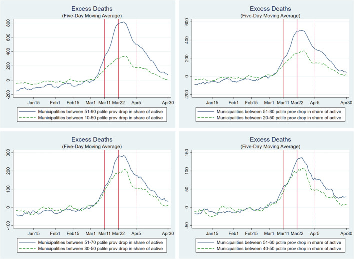
Excess deaths: subsamples by percentile drop share of active in the province. The evolution in the 5‐day moving average of excess deaths at the municipal level in the treated group (blue line) and control group (green‐dashed line) in different sub‐sample is illustrated. In the top‐left panel, the treated (control) group contains the municipalities above (below) the median and below (above) the 90th (10th) percentile with respect to the drop in the share of active population in their province between the first and second lockdowns. In the top‐right panel, the treated (control) group contains the municipalities above (below) the median and below (above) the 80th (20th) percentile with respect to the drop in the share of active population in their province between the first and second lockdowns. In the bottom‐left panel, the treated (control) group contains the municipalities above (below) the median and below (above) the 70th (30th) percentile with respect to the drop in the share of active population in their province between the first and second lockdowns. In the bottom‐right panel, the treated (control) group contains the municipalities above (below) the median and below (above) the 60th (40th) percentile with respect to the drop in the share of active population in their province between the first and second lockdowns. The two vertical lines indicate the dates of the first (March 11) and second (March 22, economic) lockdown. The dotted vertical line indicates the end of the two‐week gap after the economic lockdown (April 5)

FIGURE 4.

Excess deaths: subsamples by municipal population threshold. The evolution in the 5‐day moving average of excess deaths at the municipal level in the treated group (blue line) and control group (green‐dashed line) in different subsample below a given population threshold is illustrated. The treated (control) group contains the municipalities above (below) the median drop in the share of active population in their province between the first and second lockdowns. The two vertical lines indicate the dates of the first (March 11) and second (March 22, economic) lockdown. The dotted vertical line indicates the end of the two‐week gap after the economic lockdown (April 5)

The second alternative explanation is related to the effect of the first lockdown on mobility. Mobility is an important indicator of social interactions which, in turn, are key drivers of mortality by Covid‐19 (Fang et al., 2020; Glaeser et al., 2020; Kraemer et al., 2020). As illustrated by Figure 2, before the first lockdown, above‐the‐median municipalities had a consistently higher level of mobility (possibly because these municipalities had a higher share of active population absent lockdown measures, as also discussed in Weill et al. (2020) for the United States). At the same time, in the first lockdown period—following the shutdown of schools, restaurants, gyms, and other activities—the two groups converged in terms of mobility. This suggests that above‐the‐median municipalities experienced a stronger reduction in mobility already in the first lockdown. Indeed, as Cronin and Evans (2020) documented, a reduction in mobility takes place before the legal lockdown in response to the diffusion of the virus. Accordingly, one might argue that our estimates are due to a behavioral response in above‐the‐median municipalities, which would have led to a reduction in Covid‐19 mortality even absent any formal lockdown. Three pieces of evidence are not consistent with this argument. First, as illustrated by Table 4, in a control period in which the lagged effects of the first lockdown are likely to be already in place (we drop the first 2 weeks of the first lockdown, March 11 and March 25 as in column 4), our main estimates are still significant and the size of the coefficient is similar to that of our benchmark specification. For the first lockdown to be the driver of our effects, we should see no significant differences between above‐the‐median and below‐the‐median municipalities when comparing the (control) period March 26–April 4 with the (treatment) period April 5–April 30, as the first lockdown should already manifest its effects in terms of excess deaths in such control period. Second, also the placebo exercise shown in Table 4 (Column 5) does not support the hypothesis that our estimates are driven by a lagged effect of the first lockdown. If this was the case, we should observe a significant effect on excess deaths when comparing the first lockdown period with the 2 weeks after the beginning of the economic lockdown (when the second lockdown should not have much of an effect yet and, vice versa, a lagged effect of the first lockdown should have an arguably significant effect on excess deaths). The coefficient of such placebo exercise is smaller than the one in our baseline specification and not significant. Last but not least, as discussed in Section 4, while the activities (e.g., schools and restaurants) that closed in the first lockdown period created a substantial reduction in mobility, their overall impact in terms of contraction in active population was rather limited and, importantly, rather homogenous across municipalities, compared with the second lockdown.

Overall, while the strong reduction in mobility observed in the first lockdown period is likely to have reduced the overall mortality by Covid‐19 (Gatto et al., 2020), it does not seem to have had a differential impact in above‐the‐median versus below the median municipalities (there are no significant differences in the trends of excess deaths between the groups of municipalities in response to the first lockdown). In turn, this suggests that our measure of aggregate mobility captures a fraction of the social interactions that are relevant to the excess mortality measure. For example, although the first lockdown and the associated closure of schools is likely to have had a strong impact on mobility, it may have reflected a reduction of social interactions mainly for age groups less likely to be a source of Covid‐19 contagion (Lee & Raszka, 2020; Ludvigsson, 2020; Wu et al., 2020) and also less affected by Covid‐19 mortality (Dowd et al., 2020). In contrast, the second lockdown, and the associated reduction in mobility following the closing of all non‐essential economic activities, is likely to have mainly reflected a reduction of social interactions among workers and age groups relatively more affected by Covid‐19. Hence, aggregate changes in mobility may have different effects on Covid‐19 contagion and mortality depending on the types of social interactions they imply (see also Glaeser et al. (2020) for evidence on the heterogeneity of the impact of mobility on Covid‐19 contagion both across space and over time). ¹³ To sum up, while we cannot clearly pin‐down the exact mechanism, our main results on excess deaths are unlikely to be driven by the containment effects of the first lockdown.

6. CONCLUSIONS

In response to the Covid‐19 outbreak, most countries imposed restrictions on the movements of people and lockdowns of economic activities. In order to evaluate the effectiveness of these measures, a key challenge is the measurement of their intensity. In this paper, we focus on Italy, one of the first countries hit by the pandemic, because it offers an ideal setting to identify the causal effect of the lockdown measures on mortality by Covid‐19 (and, implicitly, on contagion). Specifically, we exploit the exogenous variation of inactive population across Italian municipalities due to the selective and progressive restriction of sectors subject to the lockdown to measure its intensity.

Our main finding is to provide an estimate of the lives saved by the tightening of the economic lockdown at the peak of the pandemic in Italy. Consistently with the evidence that Covid‐19 is particularly risky for older‐age groups, we observe a statistically significant effect for the entire population and for age groups between 40 and 64 and older (with larger and more significant effects for the cohort above 50). In addition, we find that the effectiveness of the lockdown is related to the induced reduction in people mobility: municipalities with a larger contraction of the share of active population experienced a reduction in daily mobility of 53 km per 1000 residents with respect to municipalities with a smaller contraction. A simple back of the envelope calculation indicates that the intensity of the lockdown, proxied by the reduction in the share of active population by 42.5 instead of 17 percentage points, avoided 4793 deaths in 3518 municipalities between April 5 and April 30, or 1.36 lives per municipality. A 1 percentage point reduction in the share of active population translated into a 1.32 percentage points reduction in mortality by Covid‐19.

Our results are informative of the cost‐effectiveness of lockdown measures during the first wave of the pandemic. However, the results cannot be conclusive on whether or not the severe economic lockdown has been a desirable policy on the basis of a welfare analysis. On the one hand, to assess the benefit of the lockdown in terms of economic value of reduced deaths, one would need to have detailed information on the socio‐demographic characteristics on the people that lost their life during the first pandemic wave. Unfortunately, these data are not publicly available in the Italian context. On the other hand, one would have to estimate not only the cost of the economic lockdown in terms of permanent loss of output (and thus have detailed data on the value added at the municipality‐economic sector level) but one would also have to compute the lockdown cost in terms of psychological stress suffered by the population. Hence, our analysis can be seen as a first step to address the cost‐effectiveness of the Italian lockdown. Finally it should be clear that we cannot claim the same effects in terms of avoided deaths would necessarily hold in different settings, for example when masks are available (Lyu & Wehby, 2020a) or a better contact‐tracing system is in place. More generally, our empirical strategy provides a simple methodology for future research aiming to assess the impact of the economic lockdown in reducing Covid‐19 deaths in other countries.

CONFLICTS OF INTEREST

The author declares no conflicts of interest.

Supporting information

Supplementary Material

Borri, N. , Drago, F. , Santantonio, C. , Sobbrio, F. (2021). The “Great Lockdown”: Inactive workers and mortality by Covid‐19. Health Economics, 1–16. 10.1002/hec.4383

DATA AVAILABILITY STATEMENT

The data that support the findings of this study are openly available.

REFERENCES

- Adda, J. (2016). Economic activity and the spread of viral diseases: Evidence from high frequency data. Quarterly Journal of Economics, 131(2), 891–941. [Google Scholar]
- Alvarez, F. E. , Argente, D. , & Lippi, F . (Forthcoming). A simple planning problem for Covid‐19 lockdown. American Economic Review: Insights. [Google Scholar]
- Angrist, J. D. , & Pischke, J.‐S. (2008). Mostly harmless econometrics: An empiricist’s companion. Princeton University Press. [Google Scholar]
- Barbieri, T. , Basso, G. , & Scicchitano, S. (2020). Italian workers at risk during the Covid‐19 epidemic (GLO Discussion Paper, No. 513). Global Labor Organization (GLO). [Google Scholar]
- Bartik, A. W. , Bertrand, M. , Cullen, Z. , Glaeser, E. L. , Luca, M. , & Stanton, C. (2020). The impact of Covid‐19 on small business outcomes and expectations. Proceedings of the National Academy of Sciences, 117(30), 17656–17666. [DOI] [PMC free article] [PubMed] [Google Scholar]
- Bisin, A. , & Moro, A. (2020). Learning epidemiology by doing: The empirical implications of a spatial sir model with behavioral responses. SSRN 3625361. [Google Scholar]
- Briscese, G. , Lacetera, N. , Macis, M. , & Tonin, M. (2020). Compliance with COVID‐19 social‐distancing measures in Italy: The role of expectations and duration (Working Paper 26916). National Bureau of Economic Research. [Google Scholar]
- Brooks, S. K. , Webster, R. K. , Smith, L. E. , Woodland, L. , Wessely, S. , Greenberg, N. , & Rubin, G. J. (2020). The psychological impact of quarantine and how to reduce it: Rapid review of the evidence. The Lancet. [DOI] [PMC free article] [PubMed] [Google Scholar]
- Buonanno, P. , Galletta, S. , & Puca, M. (2020, forthcoming). Estimating the severity of Covid‐19: Evidence from the Italian epicenter. Plos One. [DOI] [PMC free article] [PubMed] [Google Scholar]
- Chilton, S. , Nielsen, J. S. , & Wildman, J. (2020). Beyond Covid‐19: How the ‘dismal science’ can prepare us for the future. Health Economics, 29(8), 851–853. [DOI] [PMC free article] [PubMed] [Google Scholar]
- Cronin, C. J. , & Evans, W. N. (2020). Private precaution and public restrictions: What drives social distancing and industry foot traffic in the COVID‐19 era? (Working Paper 27531). National Bureau of Economic Research. [Google Scholar]
- Dowd, J. B. , Andriano, L. , Brazel, D. M. , Rotondi, V. , Block, P. , Ding, X. , Liu, Y. , & Mills, M. C. (2020). Demographic science aids in understanding the spread and fatality rates of Covid‐19. Proceedings of the National Academy of Sciences, 117(18), 9696–9698. [DOI] [PMC free article] [PubMed] [Google Scholar]
- Eichenbaum, M. S. , Rebelo, S. , & Trabandt, M. (2020). The macroeconomics of epidemics (Techical Report). National Bureau of Economic Research. [Google Scholar]
- Fang, H. , Wang, L. , & Yang, Y. (2020). Human mobility restrictions and the spread of the novel coronavirus (2019‐nCoV) in China (Technical Report). National Bureau of Economic Research. [DOI] [PMC free article] [PubMed] [Google Scholar]
- Favero, C. A. , Ichino, A. , & Rustichini, A. (2020). Restarting the economy while saving lives under Covid‐19 (Technical Report, CEPR Discussion Papers). [Google Scholar]
- Fernández‐Villaverde, J. , & Jones, C. I. (2020). Estimating and simulating a SIRD model of COVID‐19 for many countries, states, and cities (Technical Report). National Bureau of Economic Research. [DOI] [PMC free article] [PubMed] [Google Scholar]
- Galeotti, A. , & Surico, P. (2020). A user guide to Covid‐19 (Vol. 27). VOX CEPR Policy Portal. [Google Scholar]
- Gatto, M. , Bertuzzo, E. , Mari, L. , Miccoli, S. , Carraro, L. , Casagrandi, R. , & Rinaldo, A. (2020). Spread and dynamics of the Covid‐19 epidemic in Italy: Effects of emergency containment measures. Proceedings of the National Academy of Sciences, 117(19), 10484–10491. [DOI] [PMC free article] [PubMed] [Google Scholar]
- Glaeser, E. L. , Gorback, C. S. , & Redding, S. J. (2020). How much does COVID‐19 increase with mobility? Evidence from New York and four other U.S. cities (Working Paper 27519). National Bureau of Economic Research. [DOI] [PMC free article] [PubMed] [Google Scholar]
- Goodman‐Bacon, A. , & Marcus, J. (2020). Using difference‐in‐differences to identify causal effects of Covid‐19 policies. [Google Scholar]
- Guryan, J. (2001). Desegregation and black dropout rates (Working Paper 8345). National Bureau of Economic Research. [Google Scholar]
- Haushofer, J. , & Metcalf, C. J. E. (2020). Which interventions work best in a pandemic? Science, 368(6495), 1063–1065. [DOI] [PubMed] [Google Scholar]
- INPS‐INAPP . (2020). I settori economici essenziali nella fase 2: Impatto sui lavoratori e rischio di contagio (Technical Report). INPS‐INAPP. [Google Scholar]
- Istituto Superiore di Sanità . (2020). Characteristics of SARS‐CoV‐2 patients dying in Italy (Technical Report). https://www.epicentro.iss.it/en/coronavirus/bollettino/Report‐COVID‐2019_22_july_2020.pdf [Google Scholar]
- Jamison, J. , Bundy, D. , Jamison, D. , Spitz, J. , & Verguet, S. (2020). Comparing the impact on Covid‐19 mortality of self‐imposed behavior change and of government regulations across 13 countries. medRxiv. [DOI] [PMC free article] [PubMed] [Google Scholar]
- Kermack, W. O. , & McKendrick, A. G. (1927). A contribution to the mathematical theory of epidemics. Proceedings of the Royal Society of London. Series A, Containing Papers of a Mathematical and Physical Character, 115(772), 700–721. [Google Scholar]
- Kraemer, M. U. , Yang, C.‐H. , Gutierrez, B. , Wu, C.‐H. , Klein, B. , Pigott, D. M. , Du Plessis, L. , Faria, N. R. , Li, R. , Hanage, W. P. , Brownstein, J. S. , Layan, M. , Vespignani, A. , Tian, H. , Dye, C. , Pybus, O. G. , & Scarpino, S. V. (2020). The effect of human mobility and control measures on the Covid‐19 epidemic in China. Science, 368(6490), 493–497. [DOI] [PMC free article] [PubMed] [Google Scholar]
- Lauer, S. A. , Grantz, K. H. , Bi, Q. , Jones, F. K. , Zheng, Q. , Meredith, H. R. , Azman, A. S. , Reich, N. G. , & Lessler, J. (2020). The incubation period of coronavirus disease 2019 (Covid‐19) from publicly reported confirmed cases: Estimation and application. Annals of Internal Medicine, 172(9), 577–582. [DOI] [PMC free article] [PubMed] [Google Scholar]
- Lee, B. , & Raszka, W. V. (2020). Covid‐19 transmission and children: The child is not to blame. Pediatrics, 146(2). [DOI] [PubMed] [Google Scholar]
- Ludvigsson, J. F. (2020). Children are unlikely to be the main drivers of the Covid‐19 pandemic – A systematic review. Acta Paediatrica, 109(8), 1525–1530. [DOI] [PMC free article] [PubMed] [Google Scholar]
- Lyu, W. , & Wehby, G. L. (2020a). Community use of face masks and Covid‐19: Evidence from a natural experiment of state mandates in the US. Health Affairs, 39(8), 1419–1425. pMID: 32543923 [DOI] [PubMed] [Google Scholar]
- Lyu, W. , & Wehby, G. L. (2020b). Comparison of estimated rates of coronavirus disease 2019 (Covid‐19) in border counties in Iowa without a stay‐at‐home order and border counties in Illinois with a stay‐at‐home order. JAMA Network Open, 3(5), e2011102. [DOI] [PMC free article] [PubMed] [Google Scholar]
- McAloon, C. , Collins, Á. , Hunt, K. , Barber, A. , Byrne, A. W. , Butler, F. , Casey, M. , Griffin, J. , Lane, E. , McEvoy, D. , Wall, P. , Green, M. , O'Grady, L. , & More, S. J. , (2020). Incubation period of Covid‐19: A rapid systematic review and meta‐analysis of observational research. BMJ Open, 10(8), e039652. [DOI] [PMC free article] [PubMed] [Google Scholar]
- National Center for Health Statistics . (2020). Excess deaths associated with COVID‐19 (Technical Report). https://www.cdc.gov/nchs/nvss/vsrr/covid19/excess_deaths.htm [Google Scholar]
- Sheridan, A. , Andersen, A. L. , Hansen, E. T. , & Johannesen, N. (2020). Social distancing laws cause only small losses of economic activity during the Covid‐19 pandemic in Scandinavia. Proceedings of the National Academy of Sciences, 117(34), 20468–20473. [DOI] [PMC free article] [PubMed] [Google Scholar]
- Sun, P. , Lu, X. , Xu, C. , Sun, W. , & Pan, B. (2020). Understanding of Covid‐19 based on current evidence. Journal of Medical Virology, 92(6), 548–551. [DOI] [PMC free article] [PubMed] [Google Scholar]
- VoPham, T. , Weaver, M. D. , Hart, J. E. , Ton, M. , White, E. , & Newcomb, P. A. (2020). Effect of social distancing on Covid‐19 incidence and mortality in the US. medRxiv. [Google Scholar]
- Weill, J. A. , Stigler, M. , Deschenes, O. , & Springborn, M. R. (2020). Social distancing responses to Covid‐19 emergency declarations strongly differentiated by income. Proceedings of the National Academy of Sciences, 117(33), 19658–19660. [DOI] [PMC free article] [PubMed] [Google Scholar]
- Wilson, N. , Kvalsvig, A. , Barnard, L. T. , & Baker, M. G. (2020). Case‐fatality risk estimates for Covid‐19 calculated by using a lag time for fatality. Emerging Infectious Diseases, 26(6), 1339. [DOI] [PMC free article] [PubMed] [Google Scholar]
- Woolf, S. H. , Chapman, D. A. , Sabo, R. T. , Weinberger, D. M. , & Hill, L. (2020). Excess deaths from Covid‐19 and other causes, March‐April 2020. JAMA, 324(5), 510–513. [DOI] [PMC free article] [PubMed] [Google Scholar]
- Wu, J. T. , Leung, K. , Bushman, M. , Kishore, N. , Niehus, R. , de Salazar, P. M. , Cowling, B. J. , Lipsitch, M. , & Leung, G. M. (2020). Estimating clinical severity of Covid‐19 from the transmission dynamics in Wuhan, China. Nature Medicine, 26(4), 506–510. [DOI] [PMC free article] [PubMed] [Google Scholar]
Associated Data
This section collects any data citations, data availability statements, or supplementary materials included in this article.
Supplementary Materials