Mathematical modeling of COVID-19 transmission dynamics between healthcare workers and community

Abstract

Corona-virus disease 2019 (COVID-19) is an infectious disease that has affected different groups of humankind such as farmers, soldiers, drivers, educators, students, healthcare workers and many others. The transmission rate of the disease varies from one group to another depending on the contact rate. Healthcare workers are at a high risk of contracting the disease due to the high contact rate with patients. So far, there exists no mathematical model which combines both public control measures (as a parameter) and healthcare workers (as an independent compartment). Combining these two in a given mathematical model is very important because healthcare workers are protected through effective use of personal protective equipment, and control measures help to minimize the spread of COVID-19 in the community. This paper presents a mathematical model named SWE $I_s{I}_a$HR; susceptible individuals (S), healthcare workers (W), exposed (E), symptomatic infectious ($I_s$), asymptomatic infectious ($I_a$), hospitalized (H), recovered (R). The value of basic reproduction number $R_0$ for all parameters in this study is 2.8540. In the absence of personal protective equipment $\xi$ and control measure in the public $\theta$, the value of $R_0\approx 4.6047$ which implies the presence of the disease. When $\theta$ and $\xi$ were introduced in the model, basic reproduction number is reduced to 0.4606, indicating the absence of disease in the community. Numerical solutions are simulated by using Runge–Kutta fourth-order method. Sensitivity analysis is performed to presents the most significant parameter. Furthermore, identifiability of model parameters is done using the least square method. The results indicated that protection of healthcare workers can be achieved through effective use of personal protective equipment by healthcare workers and minimization of transmission of COVID-19 in the general public by the implementation of control measures. Generally, this paper emphasizes the importance of using protective measures.

Introduction

Corona-virus disease 2019 (COVID-19) is an infectious disease that emerged in December 2019 in China caused by a new strain of virus called severe acute respiratory syndrome coronavirus 2 (SARS COV-2)  [1], [2], [3], [4]. The first case of coronavirus disease originates from the Huanan seafood wholesale market where the live animals are being sold [5]. Coronavirus is classified among the family of coronaviridae, the order of Nidovirale, and the subfamily of Coronavirinae [6]. Alpha-coronavirus, Beta-coronavirus, Delta-coronavirus and Gamma-coronavirus are the four types of coronaviruses that belong to the subfamily orthocoronavirinae [6], [7]. Few research findings presented that origin of alpha and beta-coronavirus is from bats and rodents while avian species are the generative sources of gamma and delta-coronavirus [8].

COVID-19 can be spread from one individual to another through inhaling respiratory droplets released from the nose or mouth of an infectious individual when talking, sneezing, or coughing [9]. Also, an individual can acquire this virus through fomite transmission [10]. Older people aged 65 and above are more likely to be hospitalized or die from this disease. There is also a high severity of the disease to the group of people with underlying medical conditions such as hypertension, diabetes, cardiovascular, chronic respiratory disease and cancer [9]. Common clinical symptoms of the disease include tiredness, dry cough and fever [11] while serious symptoms include blood pressure, loss of movement or speech, chest pain and difficulty in breathing.

The basic reproduction number $R_0$ is the term used in mathematics to indicates how contagious an infectious disease is. It also known as the estimated number of cases. $R_0$ indicates how many people on average one infected individual can infect in the entire period. If $R_0>1$ the disease will persist in the community and when $R_0<1$ the disease will die away. The value of $R_0$ for COVID-19 varies from one region to another for instance, one study conducted for all European countries revealed that the value of $R_0$ was in a range of 4.22 ± 1.69 with a maximum values of 6.33 and 5.88 in Germany and the Netherlands respectively [12]. Another study of corona-virus indicated that $R_0$ ranges 2.2–4.7 [13]. Also, one study of corona-virus disease 2019 conducted in 15 Western European countries showed that the value of $R_0$ is 2.2 [14] while another study of corona-virus conducted in Africa revealed that the value of $R_0$ is 2.37 [15].

On July 12th, 2021, COVID-19 spread to about 223 countries worldwide in which more than 188 million cases were reported with a total of 4.065 million death globally. Many research groups in different nations in the world have put much effort into developing or producing vaccines [16]. Although some vaccines have been developed, nonpharmaceutical interventions are important in minimizing the outbreak.

Modeling is an essential theoretical tool that helps in understanding, and analysis of effective control and preventive measures of different communicable diseases [16]. Many models of epidemiology divide their population into compartments in which assumptions are made about the nature and time rate of transfer among the human population [17]. These models act as a mathematical framework for studying the complexity of the dynamics of epidemiological processes [9]. A mathematical model is a major tool used to present COVID-19 transmission and its simulation can be used for predictions [16]. Some mathematical models were constructed to analyze the spreads of viruses [18]. During the outbreak of COVID-19, modeling attracted a special attention to many pharmacists, mathematician, chemists, biologists, epidemiologists [1], [2], [19], [20], [21], [22], [23], [24], [25], [26], [27]. This can be an effective approach to study, simulate and predict the mechanism and transmission of the disease.

COVID-19 has affected different groups of people such as farmers, soldiers, public drivers, educators, students, healthcare workers and many other groups. The transmission rate of this disease differs from one group to another depending on contact rate. Healthcare workers which is the most important health workforce are at a high risk of contracting the disease due to the high contact rate with patients [28]. Unavailability of diagnostic tests and an insufficient number of protective equipment put the healthcare workers at the highest risk of becoming infected and infecting others. There are some models focused on the risk of COVID-19 on healthcare workers [28], [29] and others dealt with the spread of COVID-19 between the public and frontlines taking into consideration two mutually exclusive population (i.e the public compartment alone and frontlines alone) for instance Buhat et al. [26]. The aforementioned models lack a single compartment to combine both public and healthcare workers. Another mathematical model presented an organization strategies suitable to protect the healthcare workforce through formulating a compartment of health workforce alone without including the general public [30].

Despite the fact that it is hard to separate healthcare workers from the general community, there exists no mathematical model that combines healthcare workers and the general public in a single compartment and focuses on the protection of healthcare workers against COVID-19. Protection of this important health workforce will be possible if the transmission is minimized among the health co-workers. Also, minimizing the spread of infection between the community and healthcare workers will be the other way of protecting healthcare workers. So, there is a need of having a single-compartment mathematical model which takes into account both public control measures (as a parameter) and healthcare workers (as an independent compartment). Combining these two in a given mathematical model helps in protecting healthcare workers through effective use of personal protective equipment and minimize the spread of COVID-19 infection by implementing control measures in the general public. N95 masks (N stand for non resistant to oil, N95 respirator filters out the airborne particles by 95%), isolation booths, face, and eye shields are the personal protective equipment that signifies the level of protection [28].

This study formulates and analyzes the mathematical model for COVID-19 which takes into account both public control measures (as a parameter) and healthcare workers (as an independent compartment), which is the extension of the work done by Buhat et al., Sánchez-Taltavull et al. [26], [30]. Two important parameters introduced in the model are $\theta$ to represent physical distancing, face masks, sanitation, and hygiene which minimizes COVID-19 in the community, and $\xi$ to represent effective use of personal protective equipment by healthcare workers. Furthermore, this study determines how much the transmission rate of healthcare workers influences the model output.

This paper is structured as follows. After the introduction given in Section “Introduction”, a mathematical model of COVID-19 transmission dynamics taking into account both healthcare workers as an independent compartment and public control measures as a parameter is formulated in Section “Model formulation”. The dynamics of the model are analyzed in Section “Model analysis”. The numerical results which include model simulation by using the fourth-order Runge–Kutta method, model fitting and identifiability of model parameter are performed in Section “Numerical simulation”. These results support validating theoretical results. The last section presents conclusions, discussion and the future direction.

Model formulation

This section presents model development, model assumption, model flow diagram and model equations. In model development, a general overview of the deterministic model is provided.

Model development

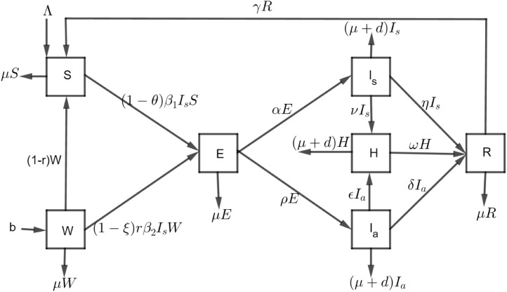
An infectious disease may spread in a complex manner when having different interacting variables. Mathematical models are among the tool used to analyze and predict the disease spread and its severity. To have a deeper insight on COVID-19 dynamics, this study formulated a biological compartmental model where the human population is divided into seven compartments: susceptible individuals (S), healthcare workers (W), exposed individuals (E), symptomatic infected individuals $\left(I_s\right)$, asymptomatic infected individuals $\left(I_a\right)$, hospitalized individuals (H) and recovered individuals (R). The total human population $N\left(t\right)$ is given by

$$N\left(t\right)=S\left(t\right)+W\left(t\right)+E\left(t\right)+I_s\left(t\right)+I_a\left(t\right)+H\left(t\right)+R\left(t\right).$$

The natural human natality rate for both susceptible and healthcare workers are $\Lambda$ and b, respectively. There is a fraction of healthcare workers which move to susceptible class. Susceptible (S) and healthcare workers population (W) get infected from enough contact with infected class $I_s$ at the rate of ${\beta }_1$ and ${\beta }_2$, respectively and then move to exposed class (E). The progression of the exposed population to symptomatic and asymptomatic infectious is at the rate of $\alpha$ and $\rho$, respectively. Symptomatic and asymptomatic infectious individuals may be hospitalized at the rate of $\nu$ and $\epsilon$, respectively. Infected individuals recover naturally or through local treatment at a rate of $\eta$ and $\delta$, respectively, but hospitalized individuals recover at a rate of $\omega$. The chance of reinfection after recovery has been considered in this model so, the recovered class can become susceptible at a rate $\gamma$. In all classes, individuals can die with a natural mortality rate $\mu$ while infected individuals ($I_s$ and $I_a$) and hospitalized humans decrease as a result of COVID-19 related death at a rate of d. In this model, there are two forces of infection which are $(1-\theta ){\beta }_1{I}_{s}S$ and $(1-\xi )r{\beta }_{2}W{I}_s$ where $\xi$ is a fraction of healthcare workers who effectively use personal protective equipment. Also, $\theta$ represents a fraction of effective use of face masks, sanitation, hygiene, and maintenance physical distancing. We assumed all aforementioned measures work best in the mass gathering when effectively implemented.

Model assumptions

Description of infectious diseases through deterministic models need to have some assumptions to be considered based on the characteristics of a specific disease under consideration. In this case, the following are some of the assumptions to be considered in formulating a COVID-19 model (1):

• i.The members of the population mix homogeneously.
• ii.Transmission is only from human to human.
• iii.Asymptotically infectious individuals are assumed to be less likely to transmit the disease since they cannot cough or sneeze as symptomatic but this is still being debated globally [31].

Model flow diagram and model equations

The model flow diagram illustrated in Fig. 1 lead to the model Eq. (1).

$$\frac{dS}{dt}=\Lambda +(1-r)W+\gamma R-(\mu +(1-\theta ){\beta }_1{I}_s)S,$$$$\frac{dW}{dt}=b-\mu W-(1-r)W-(1-\xi )r{\beta }_{2}W{I}_s,$$$$\frac{dE}{dt}=(1-\theta ){\beta }_1{I}_{s}S+(1-\xi )r{\beta }_{2}W{I}_s-(\alpha +\mu +\rho )E,$$$$\frac{d{I}_s}{dt}=\alpha E-(d+\nu +\mu +\eta )I_s,$$$$\frac{d{I}_a}{dt}=\rho E-(\mu +d+\delta +\epsilon )I_a,$$$$\frac{dH}{dt}=\nu I_s+\epsilon I_a-(\mu +d+\omega )H,$$$$\frac{dR}{dt}=\eta I_s+\omega H+\delta I_a-(\mu +\gamma )R.$$ (1)

The system of Eq. (1) is subjected to the initial conditions: $S\left(0\right)=S_0\ge 0,W\left(0\right)=W_0\ge 0,I_a\left(0\right)={\left(I_a\right)}_0\ge 0,I_s={\left(I_s\right)}_0\ge 0,E\left(0\right)=E_0\ge 0,H\left(0\right)=H_0\ge 0,R\left(0\right)=R_0\ge 0$. The parameters for the system of model (1) are described in Table 1.

Fig. 1.

Schematic diagram of COVID-19.

Table 1.

Model parameter description.

Parameter	Description
$\Lambda$	Natural natality rate of susceptible
$b$	Recruitment rate of healthcare workers
$\xi$	proportional use of personal protective equipment
${\beta }_1$	Disease transmission rate
${\beta }_2$	Transmission rate of healthcare workers
$\mu$	Natural mortality rate
$\alpha$	Progression rate from exposed stage to symptomatic infectious stage
$\rho$	Progression rate from exposed stage to asymptomatic infectious stage
$\nu$	Hospitalization rate of symptomatic infected individuals
$\epsilon$	Hospitalization rate of asymptomatic infectious individuals
$\omega$	Recovery rate of hospitalized population
$\eta$	The rate in which symptomatic infectious population recover
$\delta$	The rate in which asymptomatic infectious population recover
$d$	Disease induced death rate
$r$	proportional of healthcare workers
$\gamma$	Waning rate of disease-induced immunity
$\theta$	The rate of wearing masks, sanitation, hygiene and physical distancing

Model analysis

This section presents model properties (i.e positivity and invariant), computation of basic reproduction number, existence and uniqueness of the solution. Also, equilibria and their stability results are provided in this section.

Positivity of the solution

A population is biologically meaningful and well defined if all model solutions are non-negative for all $t\ge 0$.

Theorem 1

If the initial data $[S\left(0\right),W\left(0\right),E\left(0\right),I_s\left(0\right),I_a\left(0\right),H\left(0\right),R\left(0\right)]\ge 0$ , then the solution for S(t),W(t),E(t), $I_s\left(t\right)$ , $I_a\left(t\right)$ ,H(t),R(t) of the system of model (1) is non negative $\forall t\ge 0$ .

Proof

To prove this theorem, we used the approach in [32], where we take into account system of model (1). Consider the first equation from model (1),

$$\frac{dS}{dt}=\Lambda +(1-r)W+\gamma R-(\mu +(1-\theta ){\beta }_1{I}_s)S.$$ (2)

Omitting the first three terms and introducing inequality in Eq. (2) leads to

$$\frac{dS}{dt}\ge -(\mu +(1-\theta ){\beta }_1{I}_s)S.$$ (3)

Apply variable separable technique in Eq. (3) and introduce limit from $0$ to $t$ results

$${\int }_{S\left(0\right)}^{S\left(t\right)}\frac{dS}{S}\ge -{\int }_0^t(\mu +(1-\theta ){\beta }_1{I}_s)dt.$$

Further simplification leads to:

$$S\left(t\right)\ge S\left(0\right)e^{-(\mu +(1-\theta ){\beta }_1{I}_s)t},\text{which implies}$$

$$S\left(t\right)\ge 0.$$

This shows that the solution for susceptible population (S) is non-negative $\forall t\ge 0$.

Doing the same approach to the remaining equations in the model (1), it can be simply shown that $W\left(t\right)\ge 0,E\left(t\right)\ge 0,I_s\left(t\right)\ge 0,I_a\left(t\right)\ge 0,H\left(t\right)\ge 0,R\left(t\right)\ge 0$ for all $t\ge 0$. Therefore $(S\left(t\right),W\left(t\right),E\left(t\right),I_s\left(t\right),I_a\left(t\right),H\left(t\right),R\left(t\right))$ of the model Eq. (1) is non negative $\forall t\ge 0$. This completes the proof of Theorem 1  □

The invariant region

The invariant region describes the domain where all solutions to the model (1) are of biological and mathematical importance. All the model parameters are non-negative for all $t\ge 0$. Also, the solutions with positive initial data remain non-negative with all t$\ge 0$ and are bound.

Theorem 2

The solution set of $S\left(t\right),W\left(t\right),E\left(t\right),I_s\left(t\right),I_a\left(t\right),H\left(t\right),R\left(t\right)$ of the model Equation system (1) is confined in a positive feasible region $\varphi$ .

Proof

Suppose the feasible region $\varphi =(S\left(t\right),W\left(t\right),E\left(t\right),I_s\left(t\right),I_a\left(t\right),H\left(t\right),R\left(t\right))\in {\mathbb{R}}_{+}^7$ for $\forall t\ge 0$. At any time $t$ the total human population $N\left(t\right)$ will be: $N\left(t\right)=S\left(t\right)+W\left(t\right)+E\left(t\right)+I_s\left(t\right)+I_a\left(t\right)+H\left(t\right)+R\left(t\right)$. Differentiating with respect to $t$ leads to

$$\frac{dN}{dt}=\frac{dS}{dt}+\frac{dW}{dt}+\frac{dE}{dt}+\frac{d{I}_s}{dt}+\frac{d{I}_a}{dt}+\frac{dH}{dt}+\frac{dR}{dt}.$$ (4)

Substitute Eq. (1) into Eq. (4), further simplification result into,

$$\frac{dN}{dt}=\Lambda +b-\mu (S+W+E+I_s+I_a+H+R)-(I_s+I_a+H)d.$$ (5)

Since $N=S+W+E+I_s+I_a+H+R$, then Eq. (5) is reduced to,

$$\frac{dN}{dt}=\Lambda +b-\mu N-(I_s+I_a+H)d.$$ (6)

Assume that there is no disease-induced death for symptomatic, asymptomatic infectious, and hospitalized population due treatment in all three aforementioned classes and introducing inequality, Eq. (6) becomes

$$\frac{dN}{dt}\le \Lambda +b-\mu N.$$ (7)

Separating the variable, introducing integral on both sides for Eq. (7), and then applying limits from $0$ to $t$ gives

$${\int }_{N\left(0\right)}^{N\left(t\right)}\frac{dN}{\Lambda +b-\mu N}\le {\int }_0^{t}dt.$$

Further simplification leads to

$$N\left(t\right)\le \frac{\Lambda +b}{\mu }(1-e^{-\mu t})+N_0{e}^{-\mu t}.$$

When $t\to 0,N\left(t\right)\to N_0$ and when $t\to \infty ,N\left(t\right)\to \frac{\Lambda +b}{\mu }$. Finally $\varphi =(S,W,E,I_s,I_a,H,R)\in {\mathbb{R}}_{+}^7:0\le N\left(t\right)\le \frac{\Lambda +b}{\mu }$. The domain $\varphi$ is a positive invariant under the flow induced by the system model (1). Therefore all feasible solutions of the model (1) enter the region $\varphi$, hence the proposed COVID-19 model system (1) is well-posed and is both epidemiologically and mathematically meaningful and we consider to generate the analysis. This implies that, the model system is positive invariant in the region

$$\varphi =(S\left(t\right),W\left(t\right),E\left(t\right),I_s\left(t\right),I_a\left(t\right),H\left(t\right),R\left(t\right))\in {\mathbb{R}}_{+}^7:0\le N\left(t\right)\le \frac{\Lambda +b}{\mu },$$

for $[S\left(0\right),W\left(0\right),E\left(0\right),I_s\left(0\right),I_a\left(0\right),H\left(0\right),R\left(0\right)]\ge 0\in \varphi$ and this completes the proof. □

Existence and uniqueness for $SWE{I}_s{I}_{a}HR$ model solution

Consider the ordinary differential equation in the form of

$$\frac{dy}{dt}=f(t,y),y\left(t_0\right)=y_0.$$ (8)

By using Eq. (8) the interest will be to determine the condition that will lead the solution to be existing and condition to impose in order to have a unique solution.

This study applied the following two theorems to establish the existence and uniqueness of the solution of this model (1).

Theorem 3 Uniqueness of Solution —

As proposed in [33] , Let D denote the domain:

$$\mid t-t_0\mid \le a,\mid \mid y-y_0\mid \mid \le b,y=(y_1,y_2,\dots ,y_n),y_0=(y_1{}_0,y_2{}_0,\dots ,y_n{}_0).$$ (9)

Suppose that $f(t,y)$ satisfies the Lipschitz condition:

$$\mid \mid f(t,y_2)-f(t,y_1)\mid \mid \le k\mid \mid y_2-y_1\mid \mid ,$$ (10)

and whenever the pair of $(t,y_1)$ and $(t,y_2)$ belong to the domain D, where $k$ represents a non-negative constant. Then, there exist a constant $\delta >0$ such that there exists a unique (exactly one) continuous vector solution $y\left(t\right)$ of the system (9) in the interval $\mid t-t_0\mid \le \delta$ . It is important to note that condition (10) is satisfied by the requirement that:

$$\left\{\begin{array}{c}\frac{\partial f_i}{\partial y_j},i,j=1,2,\dots ,n,\hfill \end{array}\right)$$

be continuous and bounded in the domain D.

Lemma 1

If$f(t,y)$has continuous partial derivative$\frac{\partial f_i}{\partial y_j}$on a bounded closed convex domain$\mathbb{R}$. The interest is on the domain:

$$1<\epsilon <\mathbb{R}.$$ (11)

So we look for a bounded solution of the form$0<\mathbb{R}<\infty$as proposed in the study [33] . In proving Lemma 1 we need to consider Theorem 4 .

Theorem 4 Existence of the Solution —

Let D denotes the domain defined in(9)such that Eqs. (10), (11) hold. Then there exists a solution of a model system of Eq. (1) in our model system, which is bounded in the domain D. Consider the system of Eq. (1) ;

$$F_1=\Lambda +\gamma R+(1-r)W-(\mu +(1-\theta ){\beta }_1{I}_s)S,$$$$F_2=b-\mu W-(1-r)W-(1-\xi )r{\beta }_{2}W{I}_s,$$$$F_3=(1-\theta ){\beta }_1{I}_{s}S+(1-\xi )r{\beta }_{2}W{I}_s-(\alpha +\mu +\rho )E,$$$$F_4=\alpha E-(d+\nu +\mu +\eta )I_s,$$$$F_5=\rho E-(\mu +d+\delta +\epsilon )I_a,$$$$F_6=\nu I_s+\epsilon I_a-(\mu +d+\omega )H,$$$$F_7=\eta I_s+\omega H+\delta I_a-(\mu +\gamma )R.$$ (12)

Proof

Consider the first equation of the system of Eq. (12) for the sake of proving this,

$$F_1=\Lambda +\gamma R+(1-r)W-(\mu +(1-\theta ){\beta }_1{I}_s)S.$$ (13)

We need to show that Eq. (13) is continuous and bounded by determining the partial derivatives of $F_1$ with respect to all state variables (S, W, E , $I_s$, $I_a$,H, R).

$$\frac{\partial F_1}{\partial S}=-(\mu +(1-\theta ){\beta }_1{I}_s),\left|\frac{\partial F_1}{\partial S}\right|=|-(\mu +(1-\theta ){\beta }_1{I}_s)|<\infty ,$$

$$\frac{\partial F_1}{\partial W}=1-r,\left|\frac{\partial F_1}{\partial W}\right|=|1-r|<\infty ,$$

$$\frac{\partial F_1}{\partial E}=0,\left|\frac{\partial F_1}{\partial E}\right|=\left|0\right|<\infty ,$$

$$\frac{\partial F_1}{\partial I_s}=(1-\theta ){\beta }_{1}S,\left|\frac{\partial F_1}{\partial I_s}\right|=\left|(1-\theta ){\beta }_{1}S\right|<\infty ,$$

$$\frac{\partial F_1}{\partial I_a}=0,\left|\frac{\partial F_1}{\partial I_a}\right|=\left|0\right|<\infty ,$$

$$\frac{\partial F_1}{\partial H}=0,\left|\frac{\partial F_1}{\partial H}\right|=\left|0\right|<\infty ,$$

$$\frac{\partial F_1}{\partial R}=\gamma ,\left|\frac{\partial F_1}{\partial R}\right|=\left|\gamma \right|<\infty .$$

All partial derivatives of Eq. (13) verify that the given solution is continuous and bounded. Similarly, taking partial derivatives to the remaining equations in a model system (12) as applied in Eq. (13) will lead to the proof of continuity and boundedness of their solutions. Therefore basing the prove of Eq. (13), we conclude that all partial derivatives of Eq. (12) are continuous and bounded, hence, by Theorem 3, we can say that there exists a unique solution of Eq. (1) in the region D which is the proof of the theorem. □

Disease free equilibrium solution

The point where there is no disease is referred to as a disease-free equilibrium. We obtain this point by equating the right-hand side of all system of Eq. (1) equal to zero and substituting $E=I=H=R=0$ in all equations. let $F_0$ be the disease-free point, therefore $F_0=\left(S^0,W^0,E^0,I_s^0,I_a^0,H^0,R^0\right)=\left(\frac{b\left(1-r\right)+\Lambda \left(\mu +r-1\right)}{\mu \left(\mu -r+1\right)},\frac{b}{\mu +1-r},0,0,0,0,0\right)$.

Basic reproduction number

The basic reproduction number is defined as the expected number of COVID-19 cases created by a single COVID-19 infected individual in the population during the entire period of infectiousness. In this model, the basic reproduction number is computed using the next generation approach in [34]. The matrix F denotes the generation of new infections while matrix V denotes the disease transfer among compartments evaluated at disease-free equilibrium.

$$F=\left(\begin{array}{cccc}\hfill 0\hfill & \hfill {\beta }_1(1-\theta )\left(\frac{\Lambda (\mu +1-r)+b(1-r)}{\mu (\mu +1-r)}\right)+\frac{(1-\xi )r{\beta }_{2}b}{\mu +1-r}\hfill & \hfill 0\hfill & \hfill 0\hfill \\ \hfill 0\hfill & \hfill 0\hfill & \hfill 0\hfill & \hfill 0\hfill \\ \hfill 0\hfill & \hfill 0\hfill & \hfill 0\hfill & \hfill 0\hfill \\ \hfill 0\hfill & \hfill 0\hfill & \hfill 0\hfill & \hfill 0\hfill \end{array}\right),$$

on other hand,

$$V=\left(\begin{array}{cccc}\hfill \alpha +\mu +\rho \hfill & \hfill 0\hfill & \hfill 0\hfill & \hfill 0\hfill \\ \hfill -\alpha \hfill & \hfill d+\eta +\mu +\nu \hfill & \hfill 0\hfill & \hfill 0\hfill \\ \hfill -\rho \hfill & \hfill 0\hfill & \hfill d+\delta +\mu +\epsilon \hfill & \hfill 0\hfill \\ \hfill 0\hfill & \hfill -\nu \hfill & \hfill -\epsilon \hfill & \hfill d+\mu +\omega \hfill \end{array}\right).$$

Basic reproduction number is the spectral radius of the next-generation matrix, thus

$$R_0=\rho \left(F{V}^{-1}\right)=max({\lambda }_1,{\lambda }_2).$$

$$R_0=\frac{\alpha {\beta }_1(\theta -1)((r-1)(b+\lambda )-\lambda \mu )+\alpha \mu (1-\xi )rb{\beta }_2}{\mu (\mu -r+1)(\alpha +\mu +\rho )(d+\eta +\mu +\nu )}.$$

Local stability of the disease free equilibrium (DFE)

Local stability of the disease-free equilibrium is investigated by using the eigenvalues which are obtained by determining the partial derivatives of the vector-valued function. An equilibrium point is asymptotically stable if the Jacobian matrix evaluated at that point has negative eigenvalues. In this paper, the Routh–Hurwitz criterion in [35] will be used to prove the local stability of the disease-free equilibrium.

Theorem 5

The disease free equilibrium of the model is locally asymptotically stable if $R_0<1$ and unstable if $R_0>1$ .

Proof

In proofing this theorem, linearization of the system of model (1) is done by computing its Jacobian matrix $J_{E_0}$. The Jacobian matrix is computed at the disease-free equilibrium point by partial derivatives of each equation in the system for state variable $S,W,E,I_s,I_a$, H and R.

$$J_{DFE}=\left(\begin{array}{ccccccc}\hfill -\mu \hfill & \hfill 1-r\hfill & \hfill 0\hfill & \hfill c_1\hfill & \hfill 0\hfill & \hfill 0\hfill & \hfill \gamma \hfill \\ \hfill 0\hfill & \hfill -(\mu -1+r)\hfill & \hfill 0\hfill & \hfill c_3\hfill & \hfill 0\hfill & \hfill 0\hfill & \hfill 0\hfill \\ \hfill 0\hfill & \hfill 0\hfill & \hfill -(\rho +\mu +\alpha )\hfill & \hfill c_2\hfill & \hfill 0\hfill & \hfill 0\hfill & \hfill 0\hfill \\ \hfill 0\hfill & \hfill 0\hfill & \hfill \alpha \hfill & \hfill 0\hfill & \hfill -c_4\hfill & \hfill 0\hfill & \hfill 0\hfill \\ \hfill 0\hfill & \hfill 0\hfill & \hfill \rho \hfill & \hfill 0\hfill & \hfill -c_5\hfill & \hfill 0\hfill & \hfill 0\hfill \\ \hfill 0\hfill & \hfill 0\hfill & \hfill 0\hfill & \hfill \nu \hfill & \hfill \epsilon \hfill & \hfill -(d+\mu +\omega )\hfill & \hfill 0\hfill \\ \hfill 0\hfill & \hfill 0\hfill & \hfill 0\hfill & \hfill \eta \hfill & \hfill \delta \hfill & \hfill \omega \hfill & \hfill -(\mu +\gamma )\hfill \end{array}\right),$$ (14)

where

$$c_1={\beta }_1(1-\theta )\frac{\Lambda (\mu +1-r)+b(1-r)}{\mu (\mu +1-r)},$$

$$c_2=\frac{(1-\xi )rb{\beta }_2}{\mu +1-r}+(1-\theta ){\beta }_1\frac{\Lambda (\mu +1-r)+(1-r)b}{\mu (\mu +1-r)},$$

$$c_3=\frac{-(1-\xi )rb{\beta }_2}{\mu +1-r},$$

$$c_4=(d+\mu +\eta +\nu ),$$

$$c_5=(\mu +d+\delta +\epsilon ).$$

It is clear that from the matrix represented by Eq. (14) the first, second, third and fourth eigenvalues are ${\lambda }_1=-\mu$, ${\lambda }_2=-(\mu +\gamma )$, ${\lambda }_3=-(\mu +r-1)$, and ${\lambda }_4=-(d+\mu +\omega )$.

Therefore the matrix (14) reduces to a (3 × 3) matrix after cancellation of respective rows and columns used to obtain the first, second, third and fourth eigenvalues seen below.

$$J_{E0}=\left(\begin{array}{ccc}\hfill -(\alpha +\mu +\rho )\hfill & \hfill \frac{{\beta }_1(1-\theta )(b(1-r)+\Lambda (\mu -r+1))}{\mu (\mu -r+1)}+\frac{(1-\xi )rb{\beta }_2}{\mu -r+1}\hfill & \hfill 0\hfill \\ \hfill \alpha \hfill & \hfill 0\hfill & \hfill -(d+\eta +\mu +\nu )\hfill \\ \hfill \rho \hfill & \hfill 0\hfill & \hfill -(d+\delta +\mu +\epsilon )\hfill \end{array}\right).$$

The characteristic polynomial is of the form

$$Z\left(\lambda \right)={\lambda }^3+a_1{\lambda }^2+a_2\lambda +a_3,$$

where, $a_1=\alpha +d+\delta +2\mu +\rho +\epsilon$,

$a_2=\frac{\alpha {\beta }_1(b(\theta (r-1)+r+1)+(\theta -1)\Lambda (-\mu +r-1)+\mu (-\mu +r-1)(\alpha +\mu +\rho )(d+\delta +\mu +\epsilon )+\alpha \mu (1-\xi )rb{\beta }_2)}{\mu (\mu -r+1)}$.

So $a_2>0$ if

$\frac{\alpha b{\beta }_1\theta (1-r)}{\mu (\mu -r+1)}+(\alpha +\mu +\rho )(d+\delta +\mu +\epsilon )>\frac{\alpha {\beta }_1(1-\theta )\Lambda (\mu -r+1)+(1-\xi )\alpha \mu rb{\beta }_2}{\mu (\mu -r+1)}$,

$a_3=\frac{\left(R_0(\alpha +\mu +\rho )(d+\eta +\mu +\nu )\right)(\alpha (d+\delta +\mu +\epsilon )-\rho (d+\eta +\mu +\nu ))}{\alpha }$.

So $a_3>0$ if $\frac{\alpha (d+\delta +\mu +\epsilon )\left(R_0(\alpha +\mu +\rho )(d+\eta +\mu +\nu )\right)}{\alpha }>\frac{\rho (d+\eta +\mu +\nu )\left(R_0(\alpha +\mu +\rho )(d+\eta +\mu +\nu )\right)}{\alpha }$.

We have got $a_1>0$, $a_2>0$ and $a_3>0$ so just need to find the condition for $a_1{a}_2-a_3>0$.

Consider the value of $a_1{a}_2-a_3$,

$$a_1{a}_2-a_3=\left(m_1-m_2\right)(\alpha +d+\delta +2\mu +\rho +\epsilon )-\alpha R_0(\alpha +\mu +\rho )(d+\delta +\mu +\epsilon )(d+\eta +\mu +\nu )+m_3.$$

The condition for $a_1{a}_2-a_3$ to be greater than zero is:

$$m_1(\alpha +d+\delta +2\mu +\rho +\epsilon )+m_3>m_1{m}_2(\alpha +d+\delta +2\mu +\rho +\epsilon )+\alpha R_0(\alpha +\mu +\rho )(d+\delta +\mu +\epsilon )(d+\eta +\mu +\nu ),$$

where

$$m_1=\frac{\alpha b{\beta }_1\theta (1-r)}{\mu (\mu -r+1)}+(\alpha +\mu +\rho )(d+\delta +\mu +\epsilon ),$$

$$m_2=\frac{\alpha {\beta }_1(1-\theta )\Lambda (\mu -r+1)+(1-\xi )\alpha \mu rb{\beta }_2}{\mu (\mu -r+1)},$$

$$m_3=\frac{\rho (d+\eta +\mu +\nu )\left(R_0(\alpha +\mu +\rho )(d+\eta +\mu +\nu )\right)}{\alpha }.$$

According to the Routh–Hurwitz criterion, the necessary and sufficient condition for the stability of any system is that all the factors of the characteristic polynomial of a system must be negative. Since the eigenvalues are negative and conditions for the Routh–Hurwitz criteria are met, therefore the disease is asymptotically stable. □

Existence of endemic equilibrium point

The endemic equilibrium point is a steady-state solution in which the disease exists in the population. This solution is obtained when we take all derivatives of Eq. (1) to be equal to zero and let its solution being represented by $D^E=(S^{\ast },W^{\ast },E^{\ast },I_s^{\ast },I_a^{\ast },H^{\ast },R^{\ast })$.

For the existence of the endemic equilibrium conditions $S^{\ast }>0,W^{\ast }>0,E^{\ast }>0,I_s^{\ast }>0,I_a^{\ast }>0,H^{\ast }>0,R^{\ast }>0$ must be satisfied.

$$I_s^{\ast }=\frac{\alpha E^{\ast }}{d+\eta +\mu +\nu },I_a^{\ast }=\frac{E^{\ast }\rho }{d+\delta +\mu +\epsilon },$$

$$W^{\ast }=\frac{b}{\mu +(1-\xi ){\beta }_2{I}_s^{\ast }r-r+1},H^{\ast }=\frac{\nu I_s^{\ast }+I_a^{\ast }\epsilon }{d+\mu +\omega },$$

$$R^{\ast }=\frac{H^{\ast }\omega +\eta I_s^{\ast }+\delta I_a^{\ast }}{(\mu +\gamma )},E^{\ast }=\frac{(1-\xi ){\beta }_2{I}_s^{\ast }r{W}^{\ast }-{\beta }_1\theta I_s^{\ast }{S}^{\ast }+{\beta }_1{I}_s^{\ast }{S}^{\ast }}{\alpha +\mu +\rho },$$

$$S^{\ast }=\frac{\Lambda -r{W}^{\ast }+\gamma R^{\ast }+W^{\ast }}{\mu -{\beta }_1\theta I_s^{\ast }+{\beta }_1{I}_s^{\ast }}.$$

In this case, the solution exists and it is unique. From these conditions, we conclude that the endemic equilibrium solution is stable if and only if $R_0>1$ exhibits persistence of COVID-19 transmission in the population.

Global stability of disease free equilibrium

This study analyzes the global stability of the disease-free equilibrium point of model (1) by using an approach presented in [36]. The model can be written in the following format:

$$\frac{d{y}_n}{dt}=B(y_n-y_{DFE})+B_1{y}_i,$$

and

$$\frac{d{y}_i}{dt}=B_2{y}_i.$$

From the two equations above $y_n$ and $y_i$ are vectors of no transmitting and transmitting compartments respectively, and $y_{DFE}$ is the vector at the disease-free equilibrium of the same length as $y_n$ where $y_n={(S,W,R)}^T,y_i={(E,I_s,I_a,H)}^T$.

$$y_{DFE}={(\frac{\Lambda (\mu +1-r)+b(1-r)}{\mu (\mu +1-r)},\frac{b}{\mu +1-r},0)}^T,\text{and}$$

$$y_n-y_{DFE}=\left(\begin{array}{c}\hfill S-\frac{\Lambda (\mu +1-r)+b(1-r)}{\mu (\mu +1-r)}\hfill \\ \hfill W-\frac{b}{\mu +1-r}\hfill \\ \hfill R\hfill \end{array}\right).$$

For global stability of DFE we need to show that matrix B has a real negative eigenvalues and $B_2$ is a Metzler matrix (i.e the off-diagonal elements of $B_2$ are non-negative, symbolically denoted by $B_2\left(y_{ij}\right)\ge 0,\forall \ne j$). From model (1) we can obtain equations with and without transmission which can be written as follows:

$$\left(\begin{array}{c}\hfill \Lambda +(1-r)W+\gamma R-(\mu +(1-\theta ){\beta }_1{I}_s)S\hfill \\ \hfill b-\mu W-(1-r)W-(1-\xi )r{\beta }_{2}W{I}_s\hfill \\ \hfill \eta I_s+\omega H+\delta I_a-(\mu +\gamma )R\hfill \end{array}\right)=B\left(\begin{array}{c}\hfill S-\frac{\lambda (\mu +1-r)+b(1-r)}{\mu (\mu +1-r)}\hfill \\ \hfill W-\frac{b}{\mu +1-r}\hfill \\ \hfill R\hfill \end{array}\right)+B_1\left(\begin{array}{c}\hfill E\hfill \\ \hfill I_s\hfill \\ \hfill I_a\hfill \\ \hfill H\hfill \end{array}\right),$$

and,

$$\left(\begin{array}{c}\hfill (1-\theta ){\beta }_1{I}_{s}S+(1-\xi )r{\beta }_{2}W{I}_s-(\alpha +\mu +\rho )E\hfill \\ \hfill \alpha E-(d+\nu +\mu +\eta )I_s\hfill \\ \hfill \rho E-(\mu +d+\delta +\epsilon )I_a\hfill \\ \hfill \nu I_s+\epsilon I_a-(\mu +d+\omega )H\hfill \end{array}\right)=B_2\left(\begin{array}{c}\hfill E\hfill \\ \hfill I_s\hfill \\ \hfill I_a\hfill \\ \hfill H\hfill \end{array}\right).$$

For compatibility of matrix B is 3 × 3, $B_1$ should be 3 × 4 and $B_2$ will be 4 × 4. Using non-transmitting elements from the Jacobian matrix of the system of the model Eq. (1) result to,

$$B=\left(\begin{array}{ccc}\hfill -\mu \hfill & \hfill 1-r\hfill & \hfill \gamma \hfill \\ \hfill 0\hfill & \hfill -(\mu +1-r)\hfill & \hfill 0\hfill \\ \hfill 0\hfill & \hfill 0\hfill & \hfill -(\mu +\gamma )\hfill \end{array}\right),B_1=\left(\begin{array}{cccc}\hfill 0\hfill & \hfill -(1-\theta ){\beta }_{1}S\hfill & \hfill 0\hfill & \hfill 0\hfill \\ \hfill 0\hfill & \hfill -(1-\xi )r{\beta }_{2}W\hfill & \hfill 0\hfill & \hfill 0\hfill \\ \hfill 0\hfill & \hfill \eta \hfill & \hfill \delta \hfill & \hfill \omega \hfill \end{array}\right),$$

$$B_2=\left(\begin{array}{cccc}\hfill -(\mu +\alpha +\rho )\hfill & \hfill (1-\theta ){\beta }_{1}S+(1-\xi )r{\beta }_{2}W\hfill & \hfill 0\hfill & \hfill 0\hfill \\ \hfill \alpha \hfill & \hfill -(\eta +\nu +\mu +d)\hfill & \hfill 0\hfill & \hfill 0\hfill \\ \hfill \rho \hfill & \hfill 0\hfill & \hfill -(d+\delta +\mu +\epsilon )\hfill & \hfill 0\hfill \\ \hfill 0\hfill & \hfill \nu \hfill & \hfill \epsilon \hfill & \hfill -(\mu +\omega +d)\hfill \end{array}\right).$$

The study found that B is a matrix whose eigenvalues are located on the main diagonal. Therefore the eigenvalues of the given matrix B (i.e $-\mu$, $(1-r+\mu )$ and $-(\mu +\gamma )$) are real, distinct and negative. Additionally, $B_2$ is a Metzler matrix since its off-diagonal elements are positive and the leading diagonal entries are negative. Therefore, the DFE of our system is globally asymptotically stable, thus we have established the following important theorem.

Theorem 6

The disease free equilibrium point is globally asymptotically stable if $R_0<1$ and unstable if $R_0>1$ .

Global stability of endemic equilibrium

This study used the logarithmic Lyapunov function to analyze the stability of endemic equilibrium as used in [37]. This logarithmic function will be in this form $P=\sum a_i(y_i-y_i^{\ast }ln\left(y_1\right))$. Where $a_i$ is a positive chosen constants, $y_i$ is population of compartment $i$ and $y_i^{\ast }$ is the equilibrium level.

$P(S,W,E,I_s,I_a,H,R)=A_1(S-S^{\ast }lnS)+A_2(W-W^{\ast }lnW)+A_3(E-E^{\ast }lnE)+A_4(I_s-I_s^{\ast }ln{I}_s)+A_5(I_a-I_a^{\ast }ln{I}_a)+A_6(H-H^{\ast }lnH)+A_7(R-R^{\ast }lnR)$. The constants $A_1$, $A_2$, $A_3$, $A_4$, $A_5$, $A_6$ and $A_7$ are non negative and the function P is chosen in such away that it is a continuous and differentiable in space $▽$.

$$\frac{dP}{dt}=\left\{\begin{array}{c}{A}_1(1-\frac{S^{\ast }}{S})\frac{dS}{dt}+A_2(1-\frac{W^{\ast }}{W})\frac{dW}{dt}\hfill \\ +A_3(1-\frac{E^{\ast }}{E})\frac{dE}{dt}+A_4(1-\frac{I_s^{\ast }}{I_s})\frac{d{I}_s}{dt}\hfill \\ +A_5(1-\frac{I_a^{\ast }}{I_a})\frac{d{I}_a}{dt}+A_6(1-\frac{H^{\ast }}{H})\frac{dH}{dt}\hfill \\ +A_7(1-\frac{R^{\ast }}{R})\frac{dR}{dt}.\hfill \end{array}\right)$$ (15)

At endemic equilibrium point,

$$\Lambda =(\mu +(1-\theta ){\beta }_1{I}_s)S^{\ast }$$

$$-\gamma R^{\ast }-(1-r)W^{\ast },b=\mu W^{\ast }+(1-r)W^{\ast }+(1-\xi )r{\beta }_2{W}^{\ast }{I}_s^{\ast },(\nu +d+\mu +\eta )=\frac{\alpha E^{\ast }}{I_s^{\ast }},(\delta +d+\mu +\epsilon )=\frac{\rho E^{\ast }}{I_a^{\ast }},$$

$$d+\mu +\omega =\frac{\nu I_s^{\ast }+\epsilon I_a^{\ast }}{H^{\ast }},(\mu +\gamma )=\frac{\eta I_s^{\ast }+\omega H^{\ast }+\delta I_a^{\ast }}{R^{\ast }},(\alpha +\mu +\rho )$$

$$=\frac{(1-\theta ){\beta }_1{I}_s^{\ast }{S}^{\ast }+(1-\xi )r{\beta }_2{W}^{\ast }{I}_s^{\ast }}{E^{\ast }}.$$

It is possible to re-write Eq. (15) using the definition of the parameters value as indicated at endemic equilibrium point above which results to

$$\frac{dP}{dt}=\left\{\begin{array}{c}{A}_1(1-\frac{S^{\ast }}{S})\text{(}(\mu +(1-\theta ){\beta }_1{I}_s)S^{\ast }\hfill \\ -\gamma R\ast -(1-r)W^{\ast }+(1-r)W+\gamma R\hfill \\ -(\mu +(1-\theta ){\beta }_1{I}_s)S\text{)}\hfill \\ +A_2(1-\frac{W^{\ast }}{W})\text{(}\mu W^{\ast }+(1-r)W^{\ast }+(1-\xi )r{\beta }_2{W}^{\ast }{I}_s^{\ast }\hfill \\ -\mu W-(1-r)W-(1-\xi )r{\beta }_{2}W{I}_s\text{)}\hfill \\ +A_3(1-\frac{E^{\ast }}{E})\text{(}(1-\theta ){\beta }_1{I}_{s}S+(1-\xi )r{\beta }_{2}W{I}_s\hfill \\ -\frac{(1-\theta ){\beta }_1{I}_s^{\ast }{S}^{\ast }+(1-\xi )r{\beta }_2{W}^{\ast }{I}_s^{\ast }}{E^{\ast }}E\text{)}\hfill \\ +A_4(1-\frac{I_s^{\ast }}{I_s})(\alpha E-\frac{\rho E^{\ast }}{I_a^{\ast }}{I}_s)\hfill \\ +A_5(1-\frac{I_a^{\ast }}{I_a})(\rho E-\frac{\rho E^{\ast }}{I_a^{\ast }}{I}_a)\hfill \\ +A_6(1-\frac{H^{\ast }}{H})(\nu I_s+\epsilon I_a-\frac{\nu I_s^{\ast }+\epsilon I_a^{\ast }}{H^{\ast }}H)\hfill \\ +A_7(1-\frac{R^{\ast }}{R})(\eta I_s+\omega H+\delta I_a-\frac{\eta I_s^{\ast }+\omega H^{\ast }+\delta I_a^{\ast }}{R^{\ast }}R).\hfill \end{array}\right)$$ (16)

Further simplification of Eq. (16) gives

$$\frac{dP}{dt}=-\mu A_1\frac{{(S-S^{\ast })}^2}{S}-b{A}_2\frac{{(W-W^{\ast })}^2}{W}+F(E,I_s,I_a,H,R),$$ (17)

where F is the balance of the right term of Eq. (17). According to the approach in [38], [39], the function F is negative when $(E,I_s,I_a,H,R)\ge 0$, thus $\frac{dP}{dt}\le 0$ or zero if $E=E^{\ast },H=H^{\ast },R=R^{\ast },I_s=I_s^{\ast },I_a=I_a^{\ast }$. By LaSalle’s invariant principle  [40] implies that in the interior of F the endemic equilibrium point $F^{\ast }$ is globally asymptotically stable when $R_0>1$. This results is summarized in the following the theorem.

Theorem 7

Endemic equilibrium $F^{\ast }$ is asymptotically stable when $R_0>1$ and unstable when $R_0<1$ .

Numerical simulation

Model simulations are carried out using the values of the parameters obtained from different existing literatures. Other parameters which are not found in the literature were assumed basing on a reasonable proportionality. This section covers sensitivity and uncertainty analysis, dynamics population simulation, stability analysis of the model, the effect of varying some parameters to study the model dynamics and identifiability of model parameters. Numerical simulation in this study is done by using Runge–Kutta fourth-order method, however there are other numerical methods for simulations of non-linear differential equations such as Milne method, Eulers’ method, Adams–Bashforth–Moulton method [15], [20], [41].

Sensitivity and uncertainty analysis

The sensitivity analysis describes how the model’s parameters influence basic reproduction number $R_0$. We performed a sensitivity analysis of $R_0$ for the model’s parameters using the method established in [42]. Normalized forward sensitivity index of $R_0$, depends on the differentiability of $R_0$ with respect to a given parameter, say M, and can be computed as:

$$X_M^{R_0}=\frac{\delta R_0}{\delta M}\frac{M}{R_0}.$$

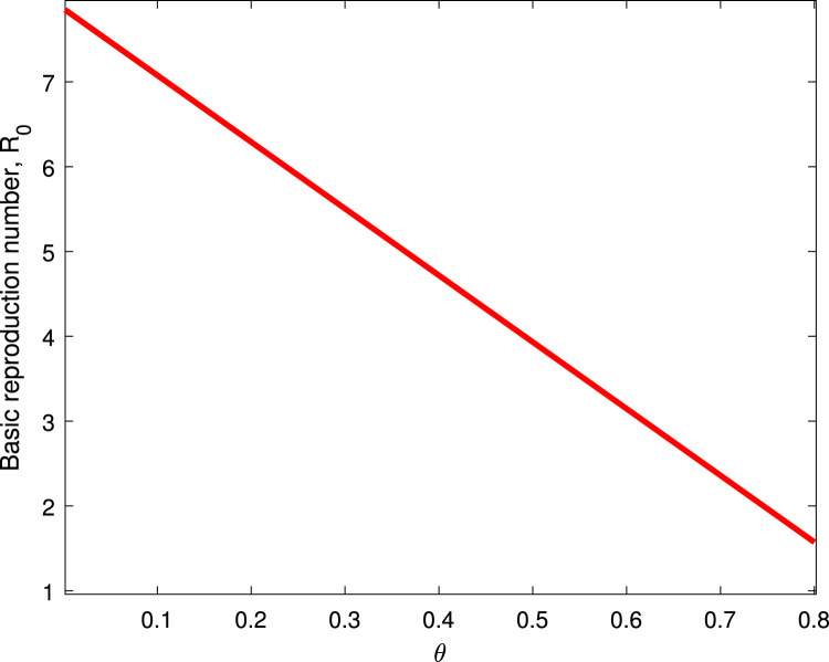
The value of basic reproduction number $R_0$ obtained using all parameters found in Table 2 is 2.8540. Also, when $\theta$=0 and $\xi$=0, $R_0$ =4.6047. When $\theta$=0.8 and $\xi$=0.9, $R_0$=0.4606. Under this note, the implementation of public control measures in the community will minimize the spread of COVID-19. Also, the effective use of personal protective equipment by the healthcare workers reduced the transmission among the healthcare workers. This implies the two aforementioned parameters are very important in suppressing the spread of COVID-19.

Table 2.

Parameter and Indices Value of the model.

Parameter	Value	Source	Indices
$\Lambda$	0.009	[43]	0.01740
$\xi$	0.7	Assumed	−0.0003
${\beta }_1$	0.5944	[31]	0.9999
${\beta }_2$	0.8	Assumed	0.0001
$\mu$	0.008	[31]	−0.9652
$\alpha$	0.6	[44]	1.9258
$\eta$	0.2	Assumed	0.2330
$\rho$	0.04	Assumed	0.0617
$\nu$	0.65	Assumed	0.7475
$b$	0.8	Assumed	0.9826
$r$	0.4	Assumed	−1.3244
$d$	0.00011	[45]	0.0001
$\theta$	0.61	Assumed	−1.5639

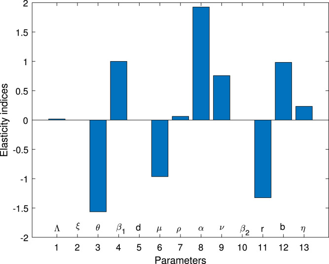
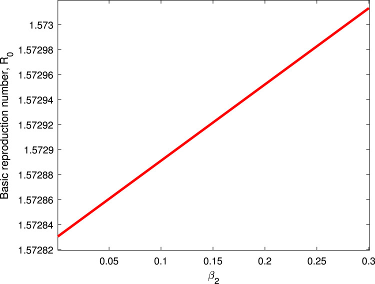
Table 2 shows the parameters value and indices for the model system (1). The most positive index is $\alpha$. This implies that increasing (decreasing) of $\alpha$ by 10% will increase (decrease) the value of $R_0$ by 19.258%. So, this parameter contributes positively to the model output $R_0$. The most negative sensitive parameter is $\theta$. This indicates that the more the population practices these measures $\theta$ keeping other parameters constant, the more the reduction of the spread of the disease. For example when the population practices $\theta$ by 10% then the value of $R_0$ will be reduced by 15.639%. Numerical indices and their signs indicated in Table 3 are also, shown in Fig. 2. Fig. 2 illustrates the parameters which can easily influence negatively or positively the spread of COVID-19. Fig. 3 depicts that control measures $\theta$ has a negative correlation with $R_0$ while Fig. 4 indicates that ${\beta }_2$ has a positive correlation with $R_0$. This implies that $\theta$ contribute negatively to the pandemic while ${\beta }_2$ contribute positively to COVID-19.

Fig. 2.

Elasticity indices for significance of parameters in $R_0$.

Fig. 3.

Effect $\theta$ on $R_0$.

Fig. 4.

Effect of ${\beta }_2$ on $R_0$.

Dynamics of populations simulation

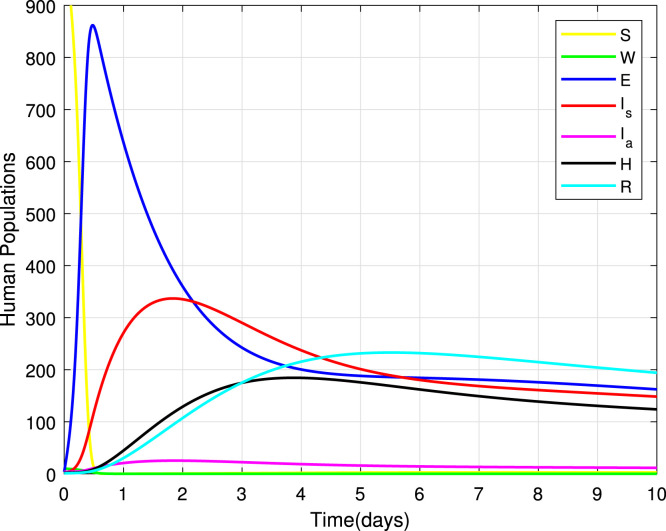
Studying the dynamics of compartments, model (1) is simulated using the Runge–Kutta method of the fourth-order. Fig. 5 indicates seven different plots to represent various human populations. The susceptible population and healthcare workers’ population decelerate exponentially to acquire endemic equilibrium levels as they die naturally or death due to a disease. Exposed, symptomatic, asymptomatic, hospitalized and recovered sub-population describes a parabola shape as it increases exponentially to attain its maximum point before decelerating exponentially to a specific endemic level.

Fig. 5.

Dynamics of SWE$I_s{I}_a$HR sub-populations.

Simulation on stability of endemic equilibrium point (EEP)

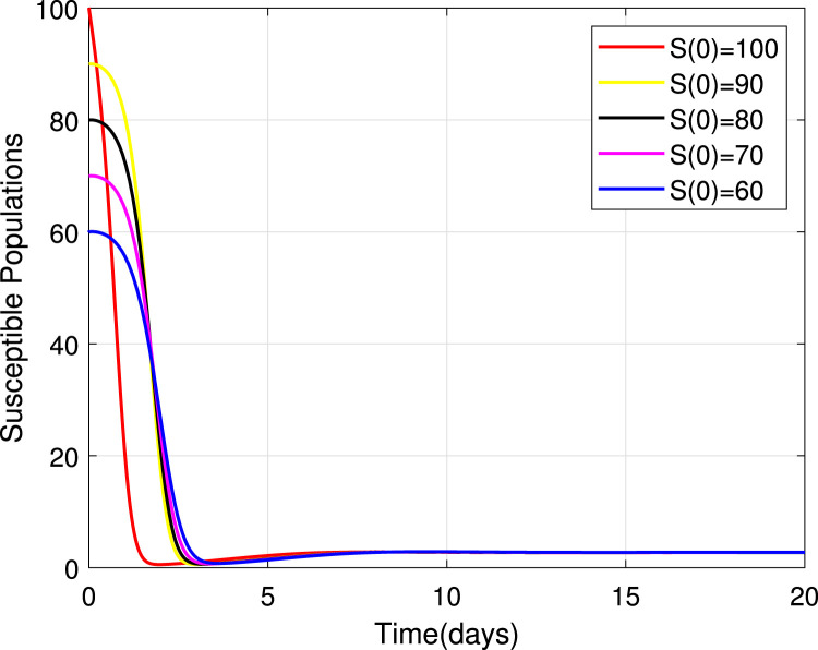
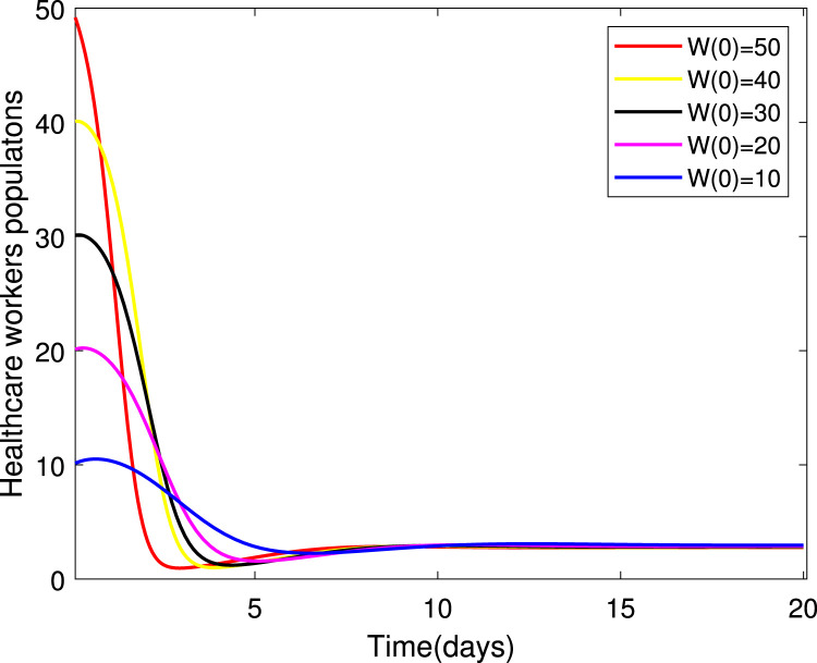
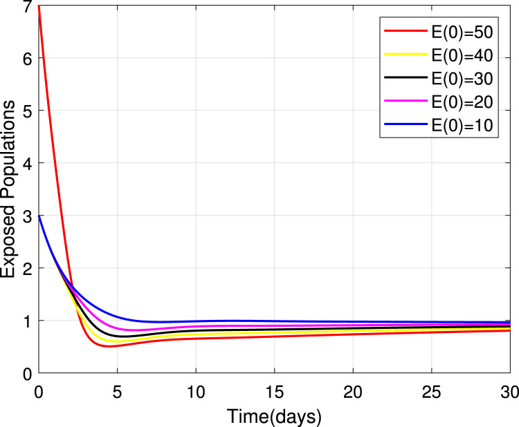
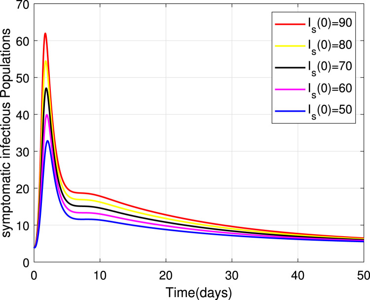
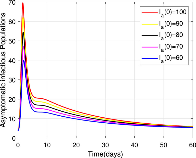
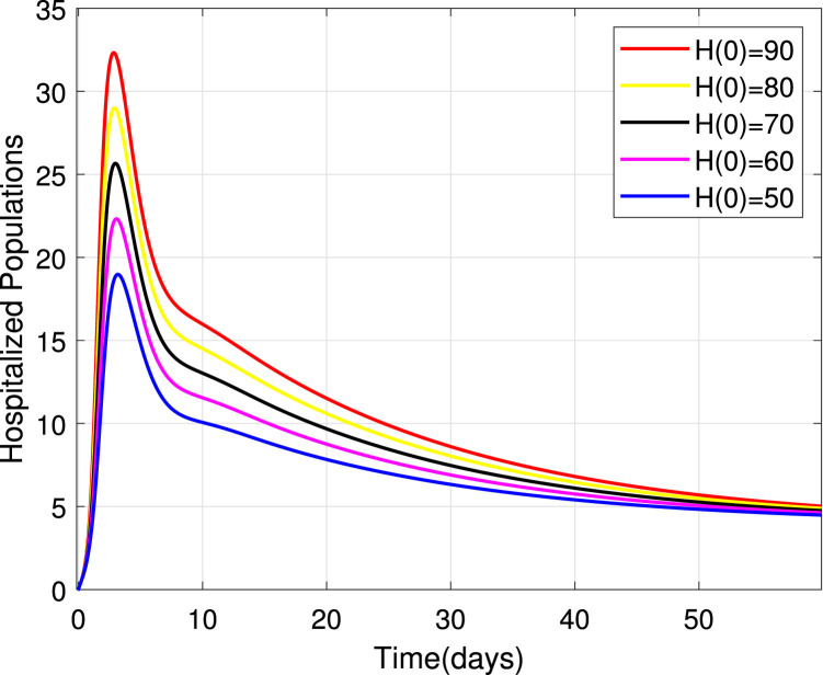
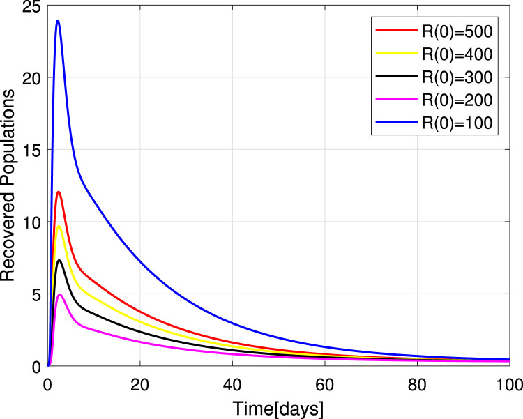
Numerical simulations for stability analysis are performed to validate analytical results. The equilibrium point is said to be globally asymptotically stable if the trajectories of the model state variables originating from different initial values vary for some time, converge to a common point and eventually maintain a constant horizontal level called an endemic equilibrium point. For this case, the trajectories are represented by red, yellow, magenta, black and blue solid plots that converge towards the equilibrium point as the time approaches infinity. Consider compartment S, suppose the initial value is (100, 90, 80, 70 and 60). Simulating model (1), we get different trajectories for S to vary at the beginning but after approaching 8 all four stabilizes. This can be observed in Fig. 6. The same interpretations can be made from other compartments as seen in Fig. 7, Fig. 8, Fig. 9, Fig. 10, Fig. 11, Fig. 12.

Fig. 6.

Stability of the EEP for susceptible population.

Fig. 7.

Stability of the EEP for healthcare workers population.

Fig. 8.

Stability of the EEP for exposed population.

Fig. 9.

Stability of the EEP for symptomatic infectious population.

Fig. 10.

Stability of the EEP for asymptomatic infectious population.

Fig. 11.

Stability of the EEP for hospitalized population.

Fig. 12.

Stability of the EEP for recovered population.

Effect of some parameters on the model

In this section, we have explored the behavior of each state variable of the proposed COVID-19 model (1). Also, profiles for state variables are graphically obtained through variation of some important parameters found in Table 2. Furthermore, mesh grid and contour plots are indicated to capture the behavior of $R_0$ with respect to some parameters

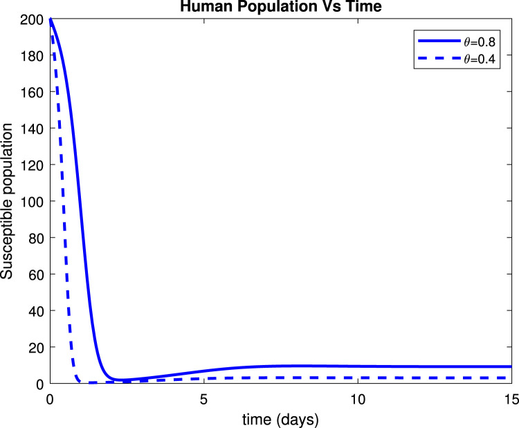
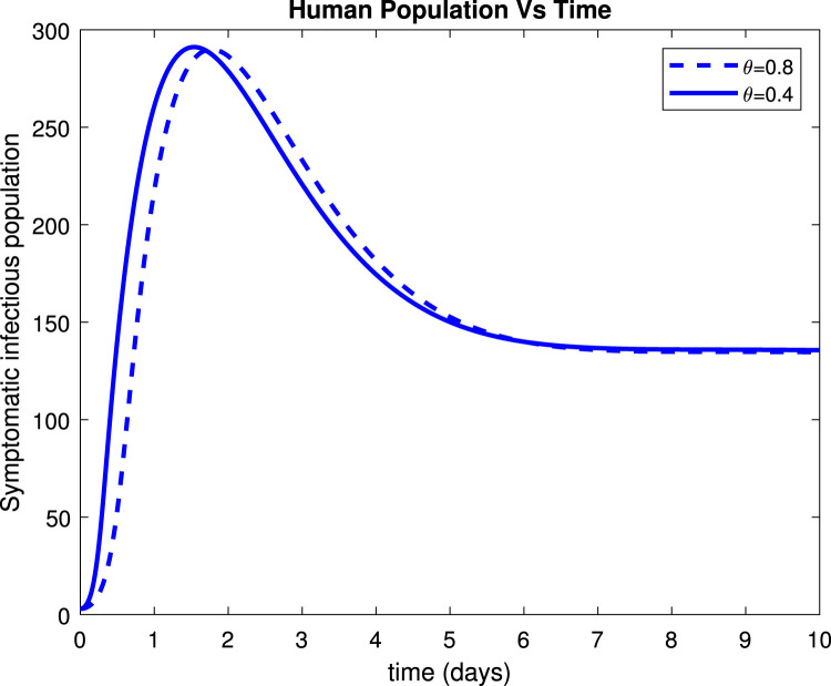
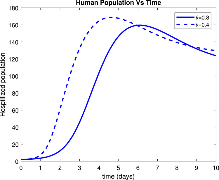
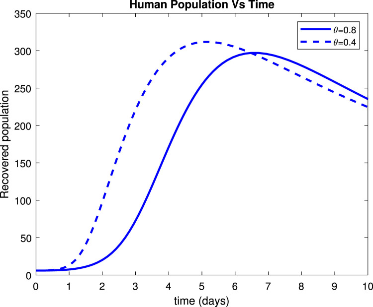
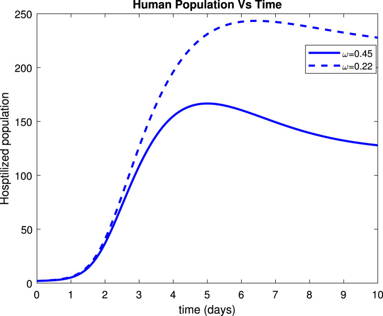
Considering the trends of Fig. 13 it can be noticed that the susceptible population increased to more than 9 people within only 15 days after implementation of control measures by 80%. Fig. 14 reveals that when implementing $\theta$ by 0.8, symptomatic infectious population reduces to below 135 patients within only 10 days. Fig. 15 shows that the number of admitted people to the hospital reduces to 130 patients after 10 days while Fig. 16 indicates that recovered increase to around 235 individuals when social distance, hygiene, and sanitation is implemented.

Fig. 13.

Effect of $\theta$ on susceptible population.

Fig. 14.

Effect of $\theta$ on symptomatic population.

Fig. 15.

Effect of $\theta$ on hospitalized humans.

Fig. 16.

Effect of $\theta$ on recovered humans.

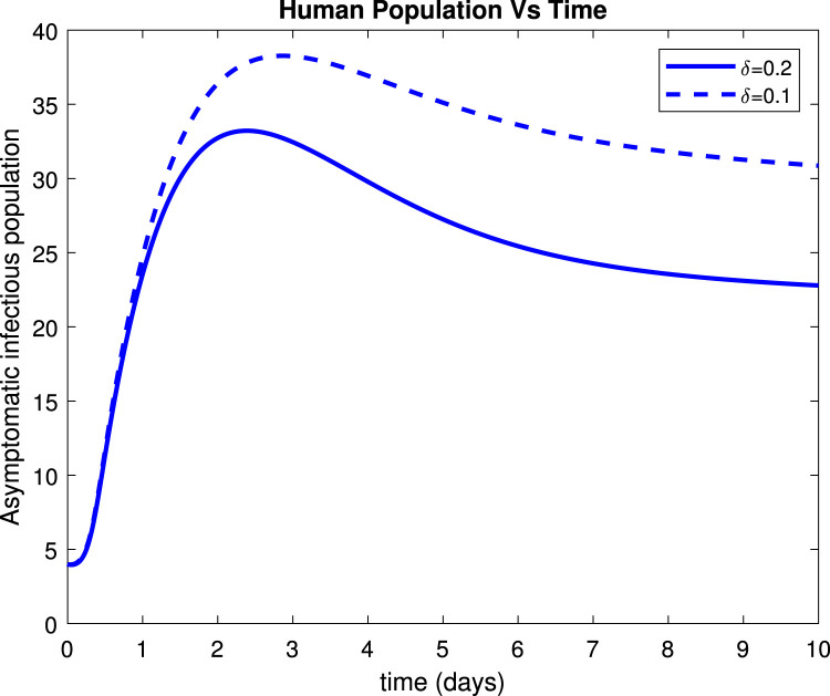
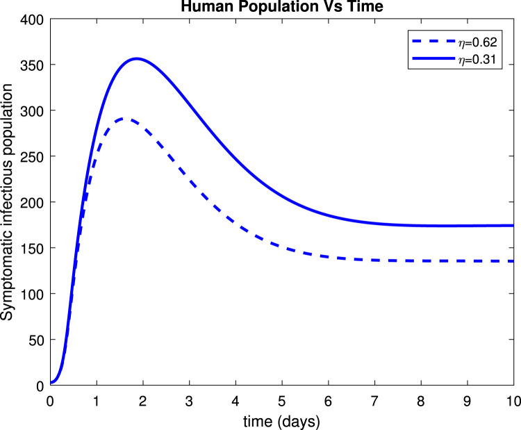
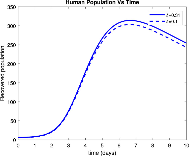
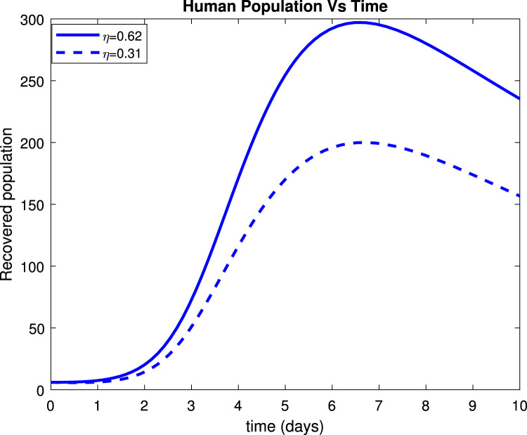
Fig. 17, Fig. 19 reveals that both asymptomatic and symptomatic infectious reduces to around 23 and 135 patients respectively, within 10 days after getting treatment. Fig. 18 shows that about 254 individuals recovered due to treatment within 10 days while Fig. 20 indicates that about 235 patients recovered due to treatment within 10 days.

Fig. 17.

Effect of treatment ($\delta$) on asymptomatic infectious population.

Fig. 19.

Effect of treatment ($\eta$) on symptomatic infectious.

Fig. 18.

Effect of treatment ($\delta$) on recovered population.

Fig. 20.

Effect of treatment ($\eta$) on recovered population.

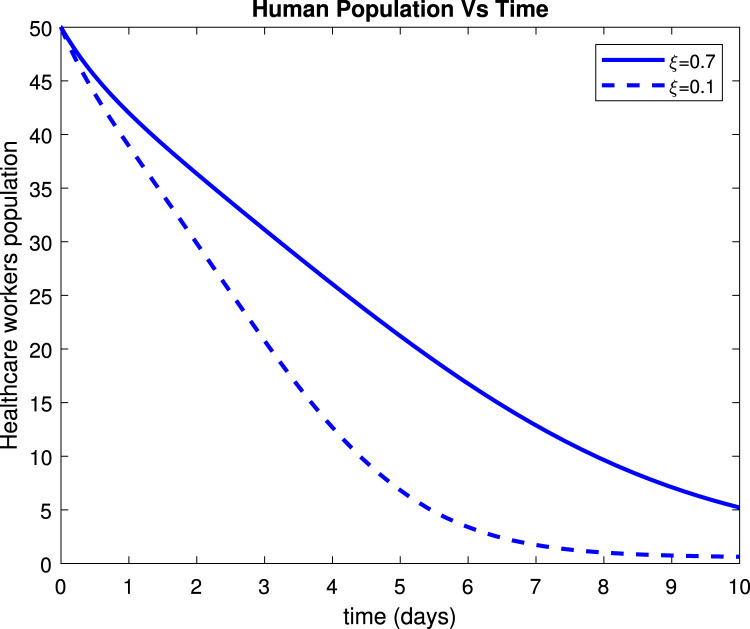
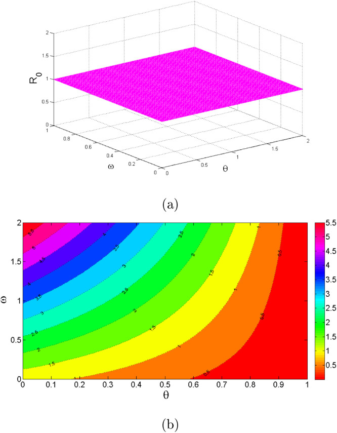
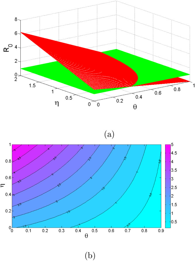
Fig. 21 depicts that the number of healthcare workers started rising after effective use of personal protective equipment. Fig. 22 shows that hospitalized individuals decrease to about 128 patients within 10 days after treatment. Also, the profile of $R_0$ versus some combination of parameters selected randomly from Table 2 via contour plots and mesh grids are shown in Fig. 23, Fig. 24.

Fig. 21.

Effect of personal protective equipment ($\xi$) on healthcare workers population.

Fig. 22.

Effect of treatment ($\omega$) on hospitalized population.

Fig. 23.

Dynamic behavior of $R_0$ for varying $\omega$ and $\theta$ on H(t).

Fig. 24.

Dynamic behavior of $R_0$ for varying $\eta$ and $\theta$ on $I_s\left(t\right)$.

Numerical results reveals that $R_0=4.6047$ which implies $R_0>1$ in absence of protective measures. Since $R_0>1$ this is a validation of analytical results of disease-free equilibrium which is an unstable and endemic point that is asymptotically stable. Also $R_0$=0.4606 in the presence of control measures in the general public and effective use of personal protective equipment by healthcare workers. Since $R_0<1$ this implies that disease-free equilibrium is asymptotically stable. This proves the importance of having control measures as well as personal protective equipment in controlling COVID-19 among the population since $R_0<1$.

Identifiability of model parameters

This subsection is devoted to the identifiability of the Parameters of the COVID-19 model (1). Some of the model (1) parameters assessed the effectiveness of the control measures in minimizing the transmission of COVID-19 in the entire community while others focused on protecting the healthcare workers for the sake of maintaining the workforce. Parameter estimation is conducted by using the least-squares method, where the idea here is to minimize the sum of squared differences between the observations and the model:

$$SS\left(\theta \right)=\sum _{i=1}^n{(y_i-f(x_i,\theta ))}^2,$$ (18)

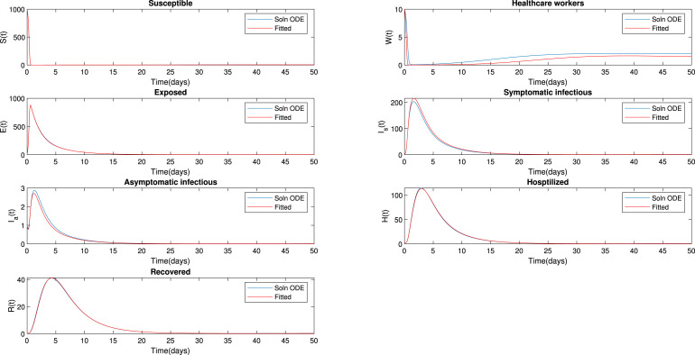
where $y_i$ is observed data of all model (1) which correspond to [$S_i,W_i,E_i,{\left(I_a\right)}_i,{\left(I_s\right)}_i,H_i,R_i$] and $f(x_i,\theta )$ is the model solution of all compartments of model (1). Table 3 indicates initial values of parameters and the model (1) optimization. Using the estimated values, the model solution can be compared with the simulated data as shown in Fig. 25. From this figure, it is observed that the simulated and fitted superimpose.

Fig. 25.

Curve fitting.

Table 3.

Parameter identifiability.

Parameter	Value	Estimate
$\Lambda$	0.009	0.0093
$\xi$	0.7	0.7269
${\beta }_1$	0.5944	0.6130
${\beta }_2$	0.8	0.8854
$\mu$	0.008	0.0082
$\alpha$	0.6	0.6368
$\eta$	0.2	0.0823
$\rho$	0.04	0.0671
$\nu$	0.65	0.4800
$b$	0.8	0.9593
$r$	0.4	0.3474
$d$	0.00011	0.0001
$\theta$	0.61	0.6160
$\omega$	0.45	0.4459
$\epsilon$	0.62	0.6325
$\delta$	0.31	0.1500
$\gamma$	0.59	0.3955

Conclusion and discussion

This paper introduced a mathematical model which consists of a system of seven non-linear ordinary differential equations. The aim of the model is to study the transmission of COVID-19 dynamics taking into account both public control measures (as a parameter) and healthcare workers (as an independent compartment). It was important to have these two parameters because we have illustrated mathematically that healthcare workers are protected through effective use of personal protective equipment and control measures are used to minimize the spread of COVID-19 in the public.

Mathematical analyses including positivity of a solution, boundedness, computation of equilibria, calculation of the basic reproduction ratio, and stability analysis of the equilibria were carried out. Numerical simulations were performed by an effective MATLAB solver ODE45 Runge–Kutta fourth-order schemes [32] and the results indicated that in the absence of both $\theta$ and $\xi$, $R_0=4.6047$. However, when the two parameters are introduced to the model, the value of $R_0$ is reduced to 0.4606. This signifies the importance of the two parameters congruently when incorporated in the model for the sake of breaking the transmission of the disease.

Conclusively, the results indicated that protection of healthcare workers can be achieved through effective use of personal protective equipment by healthcare workers and minimization of transmission of COVID-19 in the general public by the implementation of control measures. Although many healthcare workers have been using protective equipment, this work emphasizes its impacts mathematically and strongly recommend others who have not been using them to do so.

The proposed model of this paper can be further improved by considering a Fractional-order analog as well as a stochastic model in order to capture more transmission dynamics of COVID-19  [7], [23].

Funding

Not applicable.

CRediT authorship contribution statement

Lemjini Masandawa: Data curation, Writing – original draft, Methodology, Writing – review & editing, Conceptualization. Silas Steven Mirau: Visualization, Investigation, Supervision, Validation, Editing, Formal analysis, Project administration, Resource. Isambi Sailon Mbalawata: Conceptualization, Software, Preparation, Supervision, Editing, Project administration.

Declaration of Competing Interest

The authors declare that they have no known competing financial interests or personal relationships that could have appeared to influence the work reported in this paper.

Availability of data and material

All the data used in this manuscript can be found on different cited literature.

References

- 1.Ogana W., Juma V.O., Bulimo W.D. 2021. A SIRD model applied to COVID-19 dynamics and intervention strategies during the first wave in Kenya, MedRxiv. [Google Scholar]
- 2.Ivorra B., Ferrández M.R., Vela-Pérez M., Ramos A. Mathematical modeling of the spread of the coronavirus disease 2019 (COVID-19) taking into account the undetected infections. The case of China. Commun Nonlinear Sci Numer Simul. 2020;88 doi: 10.1016/j.cnsns.2020.105303. [DOI] [PMC free article] [PubMed] [Google Scholar]
- 3.Oud M.A.A., Ali A., Alrabaiah H., Ullah S., Khan M.A., Islam S. A fractional order mathematical model for COVID-19 dynamics with quarantine, isolation, and environmental viral load. Adv Difference Equ. 2021;2021(1):1–19. doi: 10.1186/s13662-021-03265-4. [DOI] [PMC free article] [PubMed] [Google Scholar]
- 4.Mahmoudi M.R., Heydari M.H., Qasem S.N., Mosavi A., Band S.S. Principal component analysis to study the relations between the spread rates of COVID-19 in high risks countries. Alex Eng J. 2021;60(1):457–464. [Google Scholar]
- 5.Sardar T., Nadim S.S., Rana S., Chattopadhyay J. Assessment of lockdown effect in some states and overall India: A predictive mathematical study on COVID-19 outbreak. Chaos Solitons Fractals. 2020;139 doi: 10.1016/j.chaos.2020.110078. [DOI] [PMC free article] [PubMed] [Google Scholar]
- 6.Hui D.S., Zumla A., Tang J.W. Lethal zoonotic coronavirus infections of humans–comparative phylogenetics, epidemiology, transmission, and clinical features of coronavirus disease 2019, The Middle East respiratory syndrome and severe acute respiratory syndrome. Curr Opin Pulm Med. 2021;27(3):146–154. doi: 10.1097/MCP.0000000000000774. [DOI] [PubMed] [Google Scholar]
- 7.Naik P.A., Yavuz M., Qureshi S., Zu J., Townley S. Modeling and analysis of COVID-19 epidemics with treatment in fractional derivatives using real data from Pakistan. Eur Phys J Plus. 2020;135(10):1–42. doi: 10.1140/epjp/s13360-020-00819-5. [DOI] [PMC free article] [PubMed] [Google Scholar]
- 8.Bozkurt F., Yousef A., Baleanu D., Alzabut J. A mathematical model of the evolution and spread of pathogenic coronaviruses from natural host to human host. Chaos Solitons Fractals. 2020;138 doi: 10.1016/j.chaos.2020.109931. [DOI] [PMC free article] [PubMed] [Google Scholar]
- 9.Peter O.J., Qureshi S., Yusuf A., Al-Shomrani M., Idowu A.A. A new mathematical model of COVID-19 using real data from Pakistan. Results Phys. 2021 doi: 10.1016/j.rinp.2021.104098. [DOI] [PMC free article] [PubMed] [Google Scholar]
- 10.Mbogo R.W., Odhiambo J.W. COVID-19 outbreak, social distancing and mass testing in Kenya-insights from a mathematical model. Afrika Mat. 2021:1–16. [Google Scholar]
- 11.Gostic K., Gomez A.C., Mummah R.O., Kucharski A.J., Lloyd-Smith J.O. Estimated effectiveness of symptom and risk screening to prevent the spread of COVID-19. Elife. 2020;9 doi: 10.7554/eLife.55570. [DOI] [PMC free article] [PubMed] [Google Scholar]
- 12.Linka K., Peirlinck M., Kuhl E. The reproduction number of COVID-19 and its correlation with public health interventions. Comput Mech. 2020;66(4):1035–1050. doi: 10.1007/s00466-020-01880-8. [DOI] [PMC free article] [PubMed] [Google Scholar]
- 13.Gill B.S., Jayaraj V.J., Singh S., Mohd Ghazali S., Cheong Y.L., Md Iderus N.H. Modelling the effectiveness of epidemic control measures in preventing the transmission of COVID-19 in Malaysia. Int J Environ Res Public Health. 2020;17(15):5509. doi: 10.3390/ijerph17155509. [DOI] [PMC free article] [PubMed] [Google Scholar]
- 14.Locatelli I., Trächsel B., Rousson V. Estimating the basic reproduction number for COVID-19 in Western Europe. Plos One. 2021;16(3) doi: 10.1371/journal.pone.0248731. [DOI] [PMC free article] [PubMed] [Google Scholar]
- 15.Yu C.-J., Wang Z.-X., Xu Y., Hu M.-X., Chen K., Qin G. Assessment of basic reproductive number for COVID-19 at global level: A meta-analysis. Medicine. 2021;100(18) doi: 10.1097/MD.0000000000025837. [DOI] [PMC free article] [PubMed] [Google Scholar]
- 16.Shahzad M., Abdel-Aty A.-H., Attia R.A., Khoshnaw S.H., Aldila D., Ali M. Dynamics models for identifying the key transmission parameters of the COVID-19 disease. Alex Eng J. 2021;60(1):757–765. [Google Scholar]
- 17.Olivares A., Staffetti E. Uncertainty quantification of a mathematical model of COVID-19 transmission dynamics with mass vaccination strategy. Chaos Solitons Fractals. 2021 doi: 10.1016/j.chaos.2021.110895. [DOI] [PMC free article] [PubMed] [Google Scholar]
- 18.Bocharov G., Volpert V., Ludewig B., Meyerhans A. vol. 245. Springer; 2018. (Mathematical immunology of virus infections). [Google Scholar]
- 19.Neto O.P., Kennedy D.M., Reis J.C., Wang Y., Brizzi A.C.B., Zambrano G.J. Mathematical model of COVID-19 intervention scenarios for São Paulo—Brazil. Nature Commun. 2021;12(1):1–13. doi: 10.1038/s41467-020-20687-y. [DOI] [PMC free article] [PubMed] [Google Scholar]
- 20.Baba I.A., Yusuf A., Nisar K.S., Abdel-Aty A.-H., Nofal T.A. Mathematical model to assess the imposition of lockdown during COVID-19 pandemic. Results Phys. 2021;20 doi: 10.1016/j.rinp.2020.103716. [DOI] [PMC free article] [PubMed] [Google Scholar]
- 21.Abdullah S.A., Owyed S., Abdel-Aty A.-H., Mahmoud E.E., Shah K., Alrabaiah H. Mathematical analysis of COVID-19 via new mathematical model. Chaos Solitons Fractals. 2021;143 doi: 10.1016/j.chaos.2020.110585. [DOI] [PMC free article] [PubMed] [Google Scholar]
- 22.Ahmed I., Modu G.U., Yusuf A., Kumam P., Yusuf I. A mathematical model of coronavirus disease (COVID-19) containing asymptomatic and symptomatic classes. Results Phys. 2021;21 doi: 10.1016/j.rinp.2020.103776. [DOI] [PMC free article] [PubMed] [Google Scholar]
- 23.Ali Z., Rabiei F., Shah K., Khodadadi T. Qualitative analysis of fractal-fractional order COVID-19 mathematical model with case study of wuhan. Alex Eng J. 2021;60(1):477–489. [Google Scholar]
- 24.Moore S., Hill E.M., Tildesley M.J., Dyson L., Keeling M.J. Vaccination and non-pharmaceutical interventions for COVID-19: a mathematical modelling study. Lancet Infect Dis. 2021 doi: 10.1016/S1473-3099(21)00143-2. [DOI] [PMC free article] [PubMed] [Google Scholar]
- 25.Contreras S., Priesemann V. Risking further COVID-19 waves despite vaccination. Lancet Infect Dis. 2021 doi: 10.1016/S1473-3099(21)00167-5. [DOI] [PMC free article] [PubMed] [Google Scholar]
- 26.Buhat C.A.H., Torres M.C., Olave Y.H., Gavina M.K.A., Felix E.F.O., Gamilla G.B. A mathematical model of COVID-19 transmission between frontliners and the general public. Netw Model Anal Health Inform Bioinform. 2021;10(1):1–12. doi: 10.1007/s13721-021-00295-6. [DOI] [PMC free article] [PubMed] [Google Scholar]
- 27.Adak D., Majumder A., Bairagi N. Mathematical perspective of Covid-19 pandemic: Disease extinction criteria in deterministic and stochastic models. Chaos Solitons Fractals. 2021;142 doi: 10.1016/j.chaos.2020.110381. [DOI] [PMC free article] [PubMed] [Google Scholar]
- 28.Dy L.F., Rabajante J.F. A COVID-19 infection risk model for frontline health care workers. Netw Model Anal Health Inform Bioinform. 2020;9(1):1–13. doi: 10.1007/s13721-020-00258-3. [DOI] [PMC free article] [PubMed] [Google Scholar]
- 29.Chatterjee K., Chatterjee K., Kumar A., Shankar S. Healthcare impact of COVID-19 epidemic in India: A stochastic mathematical model. Med J Armed Forces India. 2020;76(2):147–155. doi: 10.1016/j.mjafi.2020.03.022. [DOI] [PMC free article] [PubMed] [Google Scholar]
- 30.Sánchez-Taltavull D., Castelo-Szekely V., Candinas D., Roldán E., Beldi G. Modelling strategies to organize healthcare workforce during pandemics: application to COVID-19. J Theoret Biol. 2021;523 doi: 10.1016/j.jtbi.2021.110718. [DOI] [PMC free article] [PubMed] [Google Scholar]
- 31.Mugisha J.Y., Ssebuliba J., Nakakawa J.N., Kikawa C.R., Ssematimba A. Mathematical modeling of COVID-19 transmission dynamics in Uganda: Implications of complacency and early easing of lockdown. PLoS One. 2021;16(2) doi: 10.1371/journal.pone.0247456. [DOI] [PMC free article] [PubMed] [Google Scholar]
- 32.Yavuz M., Coşar F.O., Günay F., Özdemir F.N. A new mathematical modeling of the COVID-19 pandemic including the vaccination campaign. Open J Model Simul. 2021;9(3):299–321. [Google Scholar]
- 33.Zhang Z., Gul R., Zeb A. Global sensitivity analysis of COVID-19 mathematical model. Alex Eng J. 2021;60(1):565–572. [Google Scholar]
- 34.Van den Driessche P., Watmough J. Reproduction numbers and sub-threshold endemic equilibria for compartmental models of disease transmission. Math Biosci. 2002;180(1–2):29–48. doi: 10.1016/s0025-5564(02)00108-6. [DOI] [PubMed] [Google Scholar]
- 35.Patil A. Routh-hurwitz criterion for stability: An overview and its implementation on characteristic equation vectors using MATLAB. Emerg Technol Data Min Inf Secur. 2021:319–329. [Google Scholar]
- 36.Castillo-Chavez C., Feng Z., Huang W. On the computation of R̃ 0 and its role in global stability. IMA Vol Math Appl. 2002;125:229–250. [Google Scholar]
- 37.Korobeinikov A., Wake G.C. Lyapunov Functions and global stability for SIR, SIRS, and SIS epidemiological models. Appl Math Lett. 2002;15(8):955–960. [Google Scholar]
- 38.Korobeinikov A. Global properties of infectious disease models with nonlinear incidence. Bull Math Biol. 2007;69(6):1871–1886. doi: 10.1007/s11538-007-9196-y. [DOI] [PubMed] [Google Scholar]
- 39.McCluskey C.C. Lyapunov functions for tuberculosis models with fast and slow progression. Math Biosci Eng. 2006;3(4):603. doi: 10.3934/mbe.2006.3.603. [DOI] [PubMed] [Google Scholar]
- 40.LaSalle J.P. Dynamical systems. Elsevier; 1976. Stability theory and invariance principles; pp. 211–222. [Google Scholar]
- 41.Babaei A., Jafari H., Ahmadi M. A fractional order HIV/AIDS model based on the effect of screening of unaware infectives. Math Methods Appl Sci. 2019;42(7):2334–2343. [Google Scholar]
- 42.Carvalho D., Barbastefano R., Pastore D., Lippi M.C. 2020. A novel predictive mathematical model for COVID-19 pandemic with quarantine, contagion dynamics, and environmentally mediated transmission, medrxiv. [Google Scholar]
- 43.Mbabazi F.K., Gavamukulya Y., Awichi R., Olupot-Olupot P., Rwahwire S., Biira S. 2020. A mathematical model approach for prevention and intervention measures of the COVID–19 pandemic in Uganda. [Google Scholar]
- 44.Aldila D. Analyzing the impact of the media campaign and rapid testing for COVID-19 as an optimal control problem in East Java, Indonesia. Chaos Solitons Fractals. 2020;141 doi: 10.1016/j.chaos.2020.110364. [DOI] [PMC free article] [PubMed] [Google Scholar]
- 45.Deressa C.T., Duressa G.F. Modeling and optimal control analysis of transmission dynamics of COVID-19: The case of ethiopia. Alex Eng J. 2021;60(1):719–732. [Google Scholar]
Associated Data
This section collects any data citations, data availability statements, or supplementary materials included in this article.
Data Availability Statement