Estimation of Skin and Ocular Damage Avoided in the United States through Implementation of the Montreal Protocol on Substances that Deplete the Ozone Layer

Abstract

Overexposure to ultraviolet (UV) radiation is a threat to human health. It can cause skin cancer and cataracts. Human-made ozone-depleting substances (ODSs) reduce the ozone concentration in the Earth’s stratosphere, which acts as a protective shield from UV radiation. To protect and restore the ozone layer, the Montreal Protocol on Substances that Deplete the Ozone Layer was enacted in 1987 to phase out the production and consumption of certain ODSs and was later amended and adjusted to significantly strengthen its requirements. The United States Environmental Protection Agency (EPA) uses its Atmospheric and Health Effects Framework (AHEF) model to assess the adverse human health effects associated with stratospheric ozone depletion and the U.S. health benefits from the global implementation of the Montreal Protocol. Comparing the Montreal Protocol as amended and adjusted with a scenario of no controls on ODSs showed the prevention of an estimated 443 million cases of skin cancer and 63 million cataract cases for people born in the United States between 1890 and 2100. In addition, 2.3 million skin cancer deaths are avoided. Compared with the original 1987 Montreal Protocol, strengthening the Montreal Protocol, through its subsequent amendments and adjustments, resulted in an estimated 230 million fewer skin cancer cases, 1.3 million fewer skin cancer deaths, and 33 million fewer cataract cases.

Graphical Abstract

1. INTRODUCTION

Overexposure to ultraviolet (UV) radiation is a threat to human health, causing skin damage, eye damage, and effects on the immune system that may compromise health. Earth’s primary protection from solar UV radiation is the stratospheric ozone layer, which absorbs these high-energy UV rays before they reach Earth’s surface.

In 1974, Molina and Rowland¹ noted that human-made chlorofluoromethanes, although inert in the troposphere, release chlorine (Cl) atoms upon reaching the stratosphere and cause efficient catalytic destruction of ozone. This increases the amount of UV radiation reaching Earth’s surface, potentially causing more disease. The levels of concern rose significantly in 1985 with the unexpected discovery of the Antarctic ozone hole² and over the next decade with the realization that heterogeneous Cl chemistry can deplete substantially more ozone than gas-phase processes alone, for example, on polar stratospheric clouds³ or at midlatitudes on stratospheric aerosols,⁴ as observed after the eruption of Mt. Pinatubo.⁵

In response, the Montreal Protocol on Substances that Deplete the Ozone Layer (Montreal Protocol), an international treaty that protects the ozone layer by phasing out certain ozone-depleting substances (ODSs), was enacted in 1987. Although it was an essential and historic first step toward protecting the ozone layer, the original Montreal Protocol was insufficient relative to the damage that was being experienced; it did not control all ODSs, nor did it require a complete phaseout. Since 1987, the Montreal Protocol has been amended and adjusted numerous times to expand the list of controlled substances and to adjust the phaseout of ODS production and consumption. Notable changes include the London Amendment that required the complete phaseout of chlorofluorocarbons (CFCs), halons, and carbon tetrachloride in developed and developing countries, the Copenhagen Amendment that accelerated the timeline of complete phaseout and incorporated a hydrochlorofluorocarbon (HCFC) phaseout plan for developed countries, the Montreal Amendment that introduced an HCFC phaseout plan for developing countries, and the Beijing Amendment that tightened controls on the production and trade of HCFCs. In addition, the Montreal Adjustment of 2007 further accelerated the phaseout of HCFCs. Currently, the global transition away from ODSs and high global warming potential (GWP) substances under the Montreal Protocol is ongoing with the most recent passing of the Kigali Amendment in 2016, which phases down hydrofluorocarbons (HFCs) and came into force on January 1, 2019.

In the 1980s, the United States Environmental Protection Agency (EPA) began assessing the health impacts on the U.S. population associated with ODS-induced changes in stratospheric ozone both to better understand the adverse human health effects associated with a depleted ozone layer and to quantify the benefits of policies that reduce ODS emissions and protect stratospheric ozone. These calculations informed the development of the EPA’s Atmospheric and Health Effects Framework (AHEF) model in the 1990s. The EPA uses the AHEF to estimate the probable changes in skin cancer mortality, skin cancer incidence, and cataract incidence in the United States that result from ODS emission scenarios relative to another emission scenario or relative to a 1980 baseline, a widely used benchmark for ozone layer recovery.⁶

Health effects induced by exposure to UV radiation are primarily related to the skin, eyes, and immune system, with different health effects more closely related to different wavelengths in the UV-A (400–315 nm) and UV-B (315–280 nm) ranges. Skin effects include erythema (sunburn), aging of the skin, and various types of skin cancer: cutaneous malignant melanoma and keratinocyte cancer, including its two most common forms, squamous cell carcinoma (SCC) and basal cell carcinoma (BCC). Eye effects can include cataracts, SCC of the cornea or conjunctiva, and other damage to the surface of the eye. A cataract is the clouding of the eye’s naturally clear lens, which can cause vision impairment and blindness. Age-related cataracts have several potential causes, but lifelong exposure to UV radiation, especially UV-B rays, can play a significant role. Overexposure to UV radiation can also reduce immunological defenses, which can result in the reactivation of latent viral infections, the strengthening of skin cancers caused by viruses, and an increasing risk of infection.⁷ Of the human health effects from sun exposure, melanoma is the most lethal, causing over 7100 deaths annually in the United States.⁸ The health effects modeled in the AHEF are melanoma, BCC, SCC, and cataracts. Here we briefly describe the AHEF with its submodels and provide estimates of the health effects avoided in the U.S. by the global implementation of the Montreal Protocol compared with unchecked ozone depletion.

2. METHODS

The AHEF has five main computational steps (see Figure 1) that lead to estimated changes in the incidence and mortality for various UV-related health effects for a given ODS emission scenario. These include:

Figure 1.

Overview of AHEF submodels.

1. Emissions Submodel: Describes the past and future global emissions of 16 different ODSs that are being phased out under the Montreal Protocol.

2. Ozone Depletion Submodel: Models the impacts of ODS emissions on stratospheric ozone via changes in stratospheric chlorine and bromine.

3. UV Radiation Submodel: Models the induced instantaneous changes in ground-level UV radiation.

4. Exposure Submodel: Models the cumulative personal exposure to UV radiation by year, age, and location.

5. Effects Submodel: Uses dose–response relationships for the incidence and mortality of health effects derived from baseline incidence data and projects changes in population-based future incidence and mortality.

Many aspects of this basic methodology have been applied and presented before,^9–11 with AHEF focusing in detail on the situation in the U.S.

2.1. Emissions Submodel.

The Emissions Submodel ingests data on historical and future projected emissions, sourced from the international ozone assessment process.⁹ The AHEF defines the “baseline” incidence or mortality for skin cancer and cataracts as what would be expected to occur in the future if the concentration of stratospheric ozone remained fixed at 1980 levels. This baseline provides a standard against which to evaluate increases in mortality or incidence for these health effects from future ODS emissions and ozone depletion and, under most scenarios, the future recovery of the ozone layer to 1980 levels. Table 1 lists the three ODS emissions scenarios considered in this work. The World Meteorological Organization (WMO) A1 emissions¹³ profile accounts for the 1987 Montreal Protocol and its associated amendments and adjustments through 2007. This data set is globally recognized as representing the current state of the science. It provides species-specific ODS emissions estimates on a global scale from 1950 to 2100 and is informed by the compilation of several recently developed international ODS mixing ratio observational data sets. The historical (1950–2009) mixing ratios used are derived from a combination of (1) observations from National Oceanic and Atmospheric Administration (NOAA) and Advanced Global Atmospheric Gases Experiment (AGAGE) global sampling networks^14,15 and (2) historical mixing ratio trends derived from measured mixing ratios in firn-air samples where available and from modeled mixing ratios from the consideration of industrial production magnitudes (e.g., the Alternative Fluorocarbons Environmental Acceptability Study).¹⁶ The projected (2010–2100) mixing ratios are based on the production of ODSs reported to the United Nations Environment Programme (UNEP), estimates of the bank sizes of ODSs for 2008 from the Technology and Economic Assessment Panel,¹⁷ approved essential use exemptions for CFCs, critical-use exemptions for methyl bromide, and production estimates of methyl bromide for quarantine and preshipment use. When NOAA and AGAGE observations are available (this varies by species), the mixing ratio is an average of the two network observations. See WMO (2011)¹² table 5A-2 for more detail on the development of individual species mixing ratios. The A1 scenario was used extensively in the most recent Ozone Assessment⁶ as a benchmark for ODS atmospheric evolution. Comparisons with observations through 2016 showed that it accurately reproduced the observed total tropospheric chlorine,⁶ although with some offsetting errors because the A1 scenario slightly overestimated the rates of decline of CFCs and also the growth of HCFCs. The observed decrease in halons was also in excellent agreement with the projected values.⁶ Future updates or even entirely different scenarios can easily be implemented in AHEF. There is inherent uncertainty associated with data on ODS emissions, whether they are derived from top-down models or bottom-up models or extrapolated from atmospheric measurements.

Table 1.

Global ODS Emission Scenarios Used This Work

scenario name (abbreviation used in this work)	scenario description
Montreal Protocol as Amended and Adjusted (“WMO A1”)	ODS emissions as anticipated under the Montreal Protocol as amended and adjusted through 2007,6 which adds chemicals to those covered by the original Protocol and further regulates chemicals already covered by the original Protocol.
Montreal Protocol (“MP’87”)	ODS emissions as anticipated under the Montreal Protocol on Substances that Deplete the Ozone Layer, the original landmark international agreement of 1987.6,18
No Controls (“No Controls”)	A “Business as Usual” scenario developed by the WMO6 that envisages unregulated ODS emissions increasing continuously throughout the 21st century. The EESC grows by 3% per year.

All data sets are affected by uncertainty in emissions profiles and ODS characteristics, such as species lifetimes, transport of ODSs to the stratosphere, composition of the future atmosphere, and other factors. For the observational data used in the WMO data set, there are uncertainties due to instrument calibration and modeling errors. That said, these independent sampling programs for determining ODS global mixing ratios have substantially improved over time, with differences now typically on the order of a few percent or less (e.g., see table 1–1 of WMO (2011)¹²). In addition, uncertainty in the future emissions from ODS banks in extant products, equipment, storage containers, and landfills arises from estimates of the amount of material in the ODS banks and the rate at which the material leaks or is released from the bank. The AHEF Emissions Submodel provides the ability to modify the WMO emissions scenarios in a transparent way to conduct “what-if?” calculations to explore the health impacts of hypothetical future emissions changes (see WMO 2011).¹²

2.2. Ozone Depletion Submodel.

Calculation of ODS Concentrations.

The surface concentration of each ODS is calculated by adding the ODSs emitted each year to those remaining from the previous year. Specifically

$${\left[{\text{ODS}}_i\right]}_j={\left[{\text{ODS}}_i\right]}_{j-1}\text{exp}\left(\frac{-1}{{\tau }_i}\right)+E_{ij}{\tau }_i\left[1-\text{exp}\left(\frac{-1}{{\tau }_i}\right)\right]$$ (1)

where i is the specific ODS molecule, j is the given year, [ODS_i]_j is the atmospheric concentration of molecule i in year j (ppb mixing ratio), E_ij is the emission rate of molecule i in year j (ppb year⁻¹, converted from kt year⁻¹), and τ_i is the lifetime of the molecule i in years.

Table 2 shows the lifetimes of the various ODSs. For molecules with lifetimes longer than typical tropospheric mixing times (~1 year), surface ODS concentrations are estimated via eq 1 by multiplying their emissions by a correction factor of 1.07 (the ratio of surface to average tropospheric concentrations).¹⁹ This applies to all ODS emissions in Table 2, except for CH₃Br, for which the factor is increased to 1.16 to account also for its tropospheric chemical loss.²⁰

Table 2.

ODSs and Their Relevant Properties⁶

ODS species common name	chemical formula	lifetime (years)	fractional release factor	no. Cl atoms	no. Br atoms
CFC-11	CCl3F	52	0.47	3	0
CFC-12	CCl2F2	102	0.23	2	0
CFC-113	C2Cl3F3	93	0.29	3	0
CFC-114	C2Cl2F4	189	0.12	2	0
CFC-115	C2ClF5	540	0.04	1	0
HCFC-22	CHClF2	12	0.12	1	0
HCFC-141b	CCl2FCH3	9.4	0.34	2	0
HCFC-142b	CClF2CH3	18	0.17	1	0
halon 1301	CBrF3	72	0.28	0	1
halon 1211	CBrClF2	16	0.62	1	1
halon 2402	CBrF2CBrF2	28	0.65	0	2
halon 1202	CBr2F2	2.5	0.62	0	2
methyl bromide	CH3Br	0.8	0.6	0	1
carbon tetrachloride	CCl4	26	0.56	4	0
methyl chloroform	CH3CCl3	5	0.67	3	0
methyl chloride	CH3Cl	0.9	0.44	1	0

This procedure is repeated for each ODS, each year from 1950 to 2100, and each emission scenario, starting with zero concentration in 1950.

Calculation of EESC.

The equivalent effective stratospheric chorine (EESC) is a measure of the stratospheric inorganic halogen that is released by the ODSs and becomes available to destroy ozone.^19,21 The EESC is computed as a weighted sum of the ODSs, taking into account the number and type of halogen atoms and a fractional release factor, FRF_i, that depends on how rapidly these atoms are liberated relative to the length of time the air parcels spend in the stratosphere. These values, shown alongside the lifetimes, are estimated from models and observations¹³ and are periodically updated as improved determinations become well established.⁶

The EESC for year j is calculated as

$$\text{EESC}(j)=\sum _i{\left[{\text{ODS}}_i\right]}_{j-3}{\text{FRF}}_i\left({\text{N}}_{\text{Cl},i}+{\alpha }_i{\text{N}}_{\text{Br},i}\right)$$ (2)

A 3 year lag is assumed from the time the ODSs are emitted near the surface to the time they reach the stratosphere. Thus, in eq 2, the EESC in year j is determined by the ODS concentration 3 years earlier (j − 3). The higher ozone-destroying efficiency of bromine (relative to Cl) is parameterized by the coefficient α, which we take as 60 for midlatitude conditions.⁶

The modeled EESC values for 1980 and 1990 were 1166 and 1709 pptv, respectively, and were used to estimate the sensitivity of ozone to EESC, as detailed next. The recovery of stratospheric ozone is nominally defined to occur when the values of EESC no longer exceed those in the reference year, here taken as 1980, and is achieved in the 2040s in the A1 scenario (see the Results section) but is not projected to occur with No Controls or even under the initial Montreal Protocol phase out agreements.

Calculation of Ozone.

Considering 1980 as the reference year, the depletion of ozone in the years that follow is taken to be proportional to the EESC excess above its 1980 value. The total ozone column (TOC) in year j is thus given by

$$\text{TOC}(j,\text{ lat, }m)=\text{TOC}(1980,\text{ lat, }m)+\left[\frac{\Delta \text{TOC}(\text{lat},m)}{\Delta \text{EESC}}\right]\times [\text{EESC}(j)-\text{EESC}(1980)]$$ (3)

where the dependence on latitude (lat) and month (m) is indicated. We use TOC observations made by the Total Ozone Monitoring Spectrometer (TOMS) aboard the NASA Nimbus-7 satellite, data version 7.^22,23Figure 2 shows the TOC for the 1980 reference year (panel a) and the ΔTOC trend (panel b) based on data from late 1979 to early 1991. This trend was accompanied by a rapid increase in EESC (ΔEESC, see below), thus providing a strong “signal” to evaluate the required sensitivity ratio, ΔTOC/ΔEESC. The eruption of Mt. Pinatubo in mid-1991 confounded this relationship for several years, and more recent changes in EESC have been smaller. Thus the 1979–1991 time period allowed a straightforward estimation of the slopes in eq 3 because significant ozone depletion was observed and was associated with and attributed to strong EESC increases.

Figure 2.

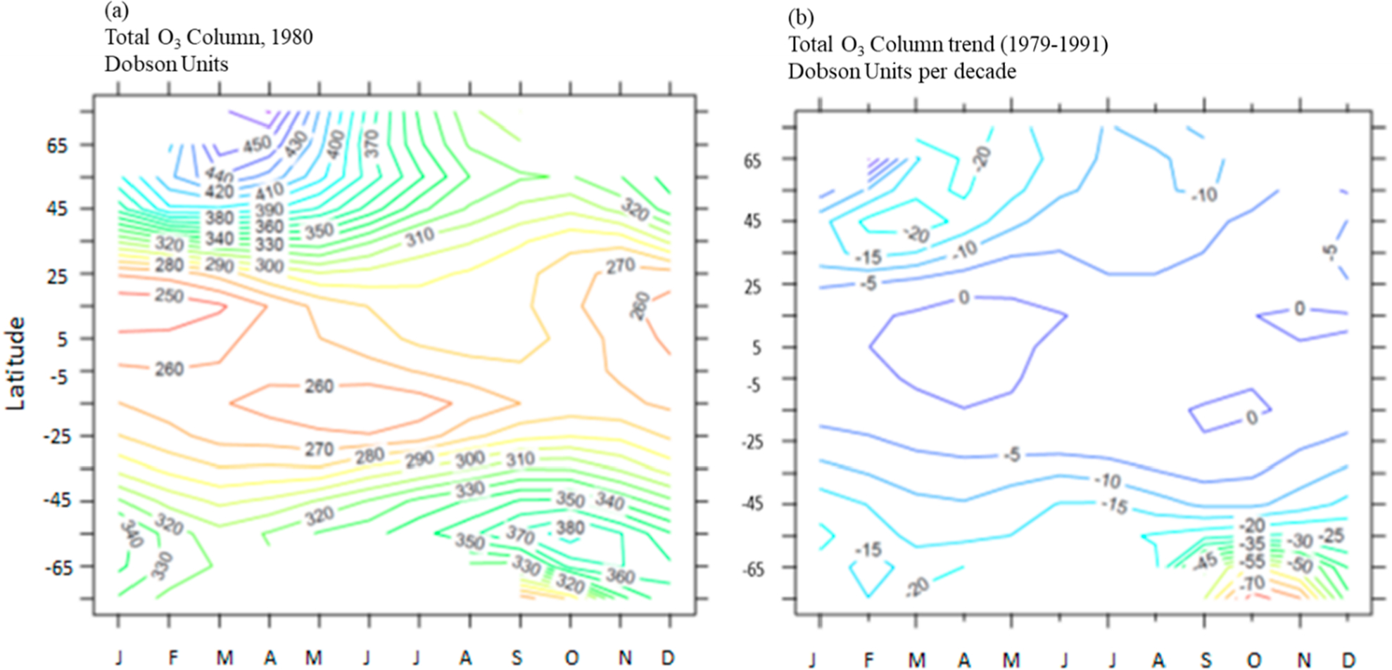
Observations from the TOMS instrument aboard the Nimbus-7 satellite of (a) the total ozone column for the reference year, 1980, and (b) the trend in the total ozone column over 1979–1991. Trends in the tropics are not statistically significant.^22,23

Equation 3 was derived for EESC exceeding its 1980 value, a condition that is met for most simulations of interest. If EESC falls below the 1980 values, then the TOC can optionally be allowed to rise above 1980 values (so-called ozone super recovery) or fixed at the 1980 values (no super recovery).

Uncertainties in the TOC trends are ~50%(2σ) or more depending on the latitude^22,23 and are a significant contributor to the overall AHEF uncertainty budget. Trends in the tropics are not significant. A minimum TOC value of 100 DU (comparable to the lowest values observed in the Antarctic ozone hole) is imposed to avoid conditions in scenarios of extreme ozone depletion, for which our parametrizations would likely fail.

2.3. UV Radiation Submodel: Calculation of Biologically Weighted UV Radiation.

Solar UV radiation incident on Earth’s surface is composed of wavelengths spanning the range of ca. 290–400 nm; over this same wavelength range, biological sensitivity to UV photons can vary by orders of magnitude. Integrating over wavelengths λ, a biologically weighted irradiance I_bio is defined as

$$I_{\text{bio}}={\int }_{\lambda }I(\lambda )A_{\text{bio}}(\lambda )\text{d}\lambda$$ (4)

where I(λ) is the sunlight’s spectral irradiance and A_bio(λ) is the action spectrum (or spectral sensitivity function) for the biological end point of interest, for example, skin cancer or cataracts. Values of I(λ) and therefore of I_bio depend on the TOC as well as the time and location, the latter mostly through their influence on the SZA (see below).

The AHEF uses the SCUP-h action spectrum (Skin Cancer Utrecht/Philadelphia data, corrected for Human transmission) to model all types of skin cancer. The SCUP spectrum was derived based on the induction of SCC in hairless mice (denoted as SCUP-m). Because mouse skin and human skin have different absorption spectra for UV light, the action spectrum was corrected for human skin transmission by adjusting to account for differences in epidermal thickness and the number of hair follicles per unit area. This adjusted action spectrum is denoted as SCUP-h.²⁴

For cataracts, the AHEF uses the Oriowo et al. action spectrum due to both its coverage of optimum wavelengths and the similarity of the pig lens to the human lens in composition and UV response.²⁵ The Oriowo et al. action spectrum is based on the in vitro induction of cataracts in whole cultured pig lenses spanning across wavelengths from 270 to 370 nm, thus extending into the UV-A spectrum. The two action spectra used in AHEF are shown in Figure 3, together with the action spectrum for the induction of sunburn in humans, which is also the basis of the widely disseminated UV Index. The spectra are normalized at 300 nm (298 nm for erythema), and their slopes in the 300–330 nm range largely determine their sensitivity to changes in TOC.²⁶

Figure 3.

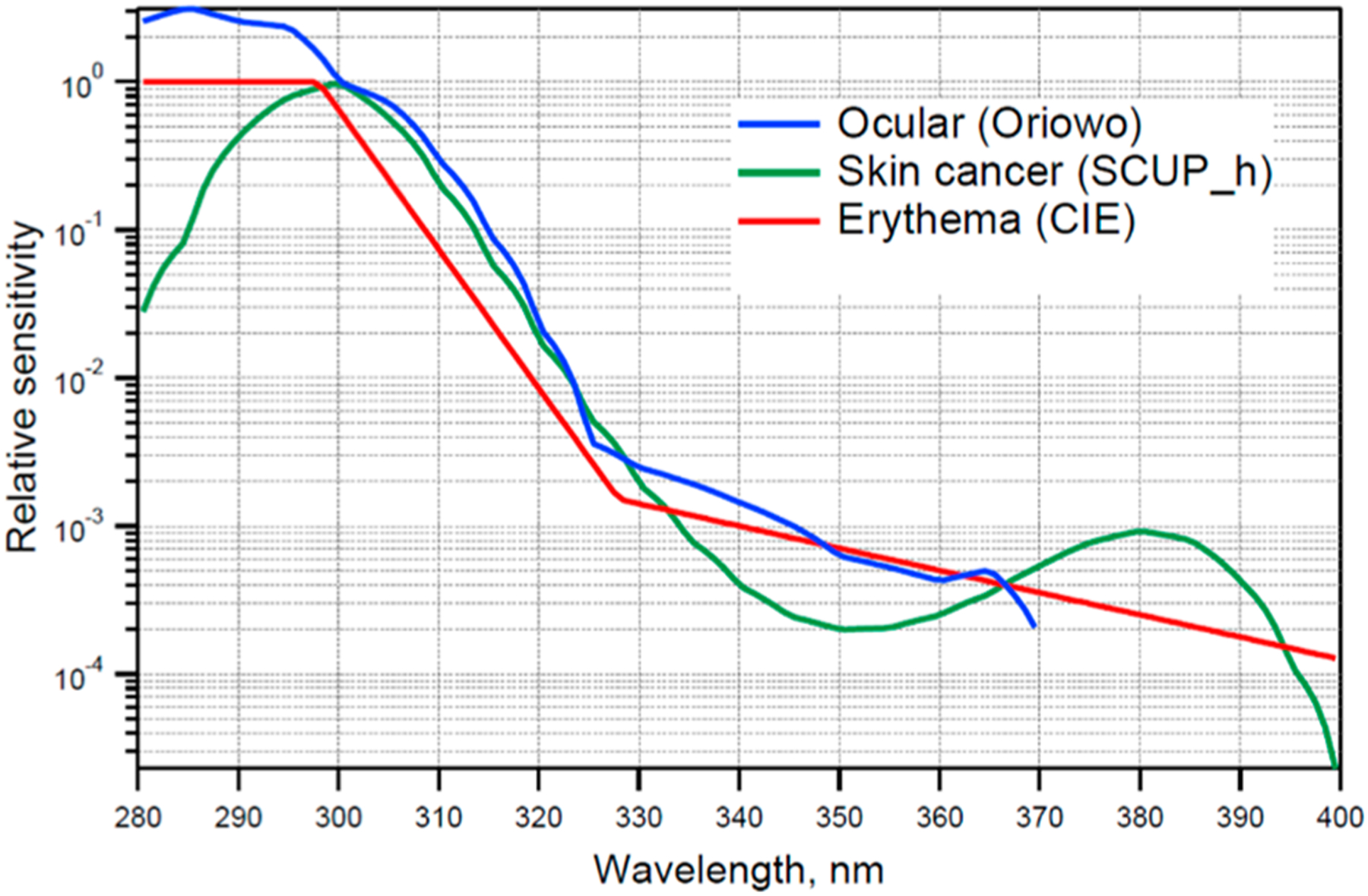
Spectral dependence (action spectra) in AHEF for the induction of skin cancer (SCUP-h, green) and cataract (ocular, blue). For comparison, the action spectrum for the induction of erythema (sunburn) in human skin is also shown, as this is the basis for computing the widely disseminated UV Index.

The ground-level spectral irradiance I(λ) is computed with the tropospheric ultraviolet–visible (TUV) model,^27,28 a radiative transfer code that computes the propagation of solar UV and visible radiation through the atmosphere. The TUV model first computes the amount of UV radiation reaching the Earth’s surface as a function of the solar zenith angle (SZA) and the atmospheric composition including the TOC; this is done at each of 120 UV wavelengths from 280 to 400 nm. Next, the ground-level irradiance of each wavelength is multiplied by the biological effectiveness (action spectrum) of that wavelength and integrated over all contributing wavelengths to yield the biologically effective irradiance in units of W m⁻². (See eq 4.) This is repeated over a grid of different solar angles and ozone columns to generate a 2D look-up table—one for each biological end point

$$I_{\text{bio }}(\text{SZA},\text{TOC})\leftarrow \text{TUV radiative transfer model }$$

The TUV model’s look-up tables are interpolated in the AHEF to estimate exposure at different locations and times and for the TOC values of the different scenarios. These interpolations are significantly more efficient computationally (albeit less flexible) than full TUV model simulations.

The TUV estimates for I_bio are for cloud-free conditions. Clouds are highly variable in space and time and can bias human exposure. They can introduce geographic dependencies that are not fully captured by the SZA and TOC, and perhaps more importantly, future UV radiation levels could be affected by changes in clouds. Climatological UV reductions by clouds range from 10 to 40% over the United States.²⁷ This is a significant element of the AHEF uncertainty budget. The inclusion of clouds in AHEF is not straightforward (in particular, future clouds), but it should at least be noted that their impact on health calculations would mostly cancel if they were assumed to remain unchanged in future scenarios.

2.4. Exposure Submodel.

Biologically weighted lifetime cumulative exposure to UV radiation is calculated by the AHEF Exposure Submodel. This submodel interpolates the TUV model’s look-up tables to find the UV dosage rate at the centroid latitude of each U.S. county, given the local TOC value for each month and year of each of the different scenarios. In practice, the model interpolates the monthly mean ozone column evaluated in Section 2.2 to each county’s centroid latitude, calculates the SZA at each centroid latitude for every daylight hour of the 15th day of the month, and interpolates from the TUV lookup table I_bio (SZA, TOC) for each latitude and hour. The individual hourly UV doses are summed into daily doses and multiplied by 30 to give monthly doses, which are then accumulated forward in time to yield time series of age-dependent cumulative UV radiation dose estimates for each birth cohort.

2.5. Effects Submodel.

The effects submodel in the AHEF determines the change in incidence that will occur based on a relative change in UV radiation dosage (i.e., the difference in the number of projected health effect cases between two policy scenarios, or between a particular policy scenario and the 1979–1980 baseline conditions). This involves three main computational steps: (1) projecting baseline incidence and mortality of health effects, (2) deriving and applying dose–response relationships for health effect incidence and mortality, and (3) projecting future health effect incidence and mortality. These computational steps also rely on historical and projected U.S. population data. For each health effect and for each future population group, estimates of the incremental health effects are computed as follows.

Evaluating eq 5 for each health effect and for each future population group produces estimates of the incremental health effects

$$\Delta \text{HEC}(\text{Pn},\text{cyr})=\text{BAF}(\text{Pn})\times \sum _{(\text{age}=0:90)}\left[{\Delta \text{UV}}_{\text{exp}}(\text{age})\times {\text{HEI}}_0(\text{Pn},\text{cyr},\text{ age })\times \text{NP}(\text{Pn},\text{cyr},\text{ age })\right]$$ (5)

where ΔHEC is the absolute increase in cases of a health effect from baseline to scenario for each population group (Pn, defined by skin type and sex) and cohort group (cyr), BAF(Pn) is the biological amplification factor for each health effect as a function of the population group, ΔUV_exp(age) is the lifetime-to-date cumulative percentage (or fractional) increase in the exposure to UV radiation, HEI₀(Pn, cyr, age) is the baseline incidence estimate of each health effect for each population group and cohort group by age, and NP(Pn, cyr, age) is the size of each population group by cohort group and age. The derivation of each of these variables is described as follows.

The standard operating assumption in the AHEF is that an individuals’ sun exposure behavior remains the same in the scenario and baseline scenario. Human behavior to sun exposure is a source of uncertainty that is not easily quantified, so the AHEF assumes that human exposure behavior remains constant through time and does not explicitly consider innovations in sun protection technology (e.g., improved sunglasses and sunscreens), increased public awareness of the effects of overexposure to UV radiation, or increased sensitization to the need for early treatment of suspicious lesions. Using the AHEF to estimate incremental health effects is less sensitive to behavioral changes over time because these may “cancel out” as long as those changes are expected to occur in both the baseline and policy scenarios.

Baseline Incidence and Mortality.

The AHEF defines “baseline” incidence and mortality as what would be expected to occur in the future if the concentration of the stratospheric ozone remained fixed at 1980 levels. The derivation of baseline rates for the U.S. population is described for each UV-related health effect.

Melanoma Incidence and Mortality.

Baseline melanoma mortality data for the years 1950–1984 were obtained from the EPA/National Cancer Institute (EPA/NCI) data set.^34,29 This data set reports the deaths from melanoma in individuals for 18 age groups (5 year birth cohorts), disaggregated by sex, skin type, and U.S. county. For modeling in the AHEF, county-level rates were regionally aggregated into three latitude bands (20°N to 30°N, 30°N to 40°N, and 40°N to 50°N). Melanoma mortality rates show a “cohort effect”, where age-specific mortality rates depend on the birth year, as shown in Figure 4 for 30–40°N. (See Figure S5 for other latitudes.) Actual and predicted mortality rates for each age group in the 1960, 1965, and 1970 birth cohorts were averaged to project future cohorts’ mortality rates. These three cohort groups were selected because they represent the most recent birth cohorts with statistically robust mortality data.

Figure 4.

Melanoma mortality baseline rates per 100 000 by sex and birth cohort for the 30°N to 40°N latitude band. Rates for other maladies and locations are presented in the Supporting Information.

Melanoma baseline incidence rates were extracted from the NCI’s Surveillance, Epidemiology, and End Results (SEER) Program.³⁵ This data set was aggregated into 18 age groups by sex, skin type, and the three U.S. latitude bands. The small size of the SEER data set necessitated a different method for projecting future incidence. The ratio of melanoma incidence to mortality was calculated and averaged over 10 years, 1984–1994, by latitude band and sex. Then, incidence-to-mortality ratios were applied to the EPA/NCI melanoma mortality rates to generate comprehensive melanoma incidence rates by age, cohort, and sex (Figure S6). For very young age groups, incidence and mortality information were quite sparse, and thus it was assumed that incidence was at least equal to mortality. Like melanoma mortality, incidence shows a cohort effect.

Keratinocyte Cancer Incidence and Mortality.

Baseline mortality data for keratinocyte cancer were obtained from the EPA/NCI data set, and the same regional aggregation and regression extrapolation procedures described for melanoma mortality were applied; the resulting baseline mortality rates are shown in Figure S7. Although ambiguities in the reporting and recording of information on death certificates (for example, if complications related to keratinocyte skin cancer hospitalizations such as infections or pneumonia are listed as the cause of death) mean that deaths may be under-reported in the EPA/ NCI data set, this is the most comprehensive data set available. A cohort effect is observed, but in contrast with melanoma, recent cohorts experience reduced keratinocyte mortality, possibly due to advances in early detection and treatment.

The AHEF uses baseline BCC and SCC incidence rates, as reported for light-skinned individuals in U.S. EPA (1987)³⁶ and Fears and Scotto (1983)³⁷ by age, region, and sex; these estimates were originally derived from Scotto et al. (1983)³⁸ based on a nationwide survey in eight cities across the United States from 1977 to 1978. Keratinocyte cancer incidence data do not display a cohort trend, and thus the age-specific baseline incidence rates are applied to all cohorts. (See Table S1.)

Cataract Incidence.

The AHEF uses cataract baseline incidence estimates derived from computing annualized change as a function of age in prevalence data presented by Congdon et al. (2004).³⁹ (See Table S2.) This study analyzed all three forms of cataracts (nuclear, posterior subcapsular, and cortical), but only the cortical cataract is clearly associated with exposure to UV radiation;³² much uncertainty exists regarding the role of UV-B rays and other forms of cataracts. Thus the AHEF model provides an upper bound of UV-induced cataract cases.

UV Dose–Response: Biological Amplification Factor.

The dose–response relation quantifies the effect of exposure to UV radiation (the dose) on the incidence of skin cancer and cataracts (the responses). Once the appropriate action spectrum is selected for each health effect and the UV radiation dose of biologically active radiation and morbidity or mortality across latitudes are identified, statistical regression analyses are used to estimate the parameters of the dose–response relationship. Several mathematical representations of the dose–response relationship are available within the AHEF, including exponential, power, and linear models

$$\begin{gathered} \text{Response }~{\text{e}}^{a\text{ Dose }}\text{\hspace{0.17em}\hspace{0.17em}\hspace{0.17em} (exponential)} \\ ~\left(\text{Dose}\right){}^b\text{ (power) } \end{gathered}$$

$$\Delta \text{Response/Response }=b\Delta \text{Dose/Dose }(\text{power, locally linear})$$

where the coefficients a or b are estimated from the statistical regression analysis. By default, the AHEF uses the locally linear power model (see eq 5), so that the coefficient b is easily identified as the percentage increase in incidence or mortality from a 1% increase in the UV dose. (b is also known as the Biological Amplification Factor, or BAF.) The BAFs used in AHEF are shown in Table 3. The BAFs were determined for the health effects of SCC and BCC by de Gruijl and Forbes (1995),³¹ melanoma for light-skinned males and females by Pitcher and Longstreth (1991)²⁹ (see also U.S. EPA, 2006),³⁰ and cataract incidence by West et al. (1998; 2005).^32,42 Tabulations of BAFs by sex, race, and health effects are used within the AHEF model, although cataracts were found to be relatively insensitive to sex. For each health effect, the AHEF applies the BAF to predict the future incidence and mortality.

Table 3.

Biological Amplification Factors (BAFs) Used in the AHEF Model

	light skin, males	light skin, female	dark skin, male	dark skin, female
melanoma incidencea	0.58 ± 0.02b	0.50 ± 0.02b	0	0
melanoma mortalitya	0.58 ± 0.02b	0.50 ± 0.02b	0	0
keratinocyte mortalitya	0.71 ± 0.03b	0.46 ± 0.03b	0	0
basal incidenceb	1.5 ± 0.5	1.3 ± 0.4	0	0
squamous incidencec	2.6 ± 0.7	2.6 ± 0.8	0	0
cataract incidenced	0.17 ± 0.09	0.17 ± 0.09	0.24 ± 0.09	0.24 ± 0.09

^aPitcher and Longstreth (1991);²⁹ EPA (2006).³⁰

^bFor melanoma incidence, melanoma mortality, and keratinocyte mortality, reported errors include only the standard error of the fit.

^cde Gruijl and Forbes (1995).³¹

^dWest et al. (2005);³² EPA (2010).³³

Uncertainties in BAFs are substantial (see Table 3) and important to the AHEF uncertainty budget. The uncertainties shown in the Table for melanoma (incidence and mortality) and keratinocyte mortality, as reported by Pitcher and Longstreth (1991)²⁹ and the EPA (2006),³⁰ refer only to the standard error.

Additional systematic errors are likely due to uncertainties in the action spectrum for the induction of melanoma as well as many other factors not considered by Pitcher and Longstreth (1991).²⁹

In determining the BAF for basal and squamous cancer incidence, de Gruijl and Forbes (1995)³¹ considered a number of confounding factors such as uncertainty in the action spectra, migration, patient reporting delay, high early life exposure, and potential exposure to other carcinogens. Thus the relative error estimates reported by de Gruijl and Forbes³¹ are also likely more representative of real-life uncertainties for melanoma and keratinocyte cancer mortality. Given the large percentage value of these uncertainties, they can be more simply summarized as multiplicative factors of ~1.3 for skin cancers and 1.7 for cataracts.

Population Data.

Population data disaggregated by race, sex, age, county, and year for the period up to 2100 are needed as inputs into the effects submodel of the AHEF. Subdivided annual data were sourced from the U.S. Census Bureau for the period of 1985–2018.^43–45 Disaggregated data was not available prior to 1985, and thus the AHEF applies the 1985 values to all prior years. Additionally, national population projections for the period 2019–2060 were obtained from the U.S. Census Bureau.^46,47 Population projections are disaggregated by race, sex, age, and year but not by county. The AHEF distributes the projected data among each county in proportion to the 2016 data distributions. Because projections are unavailable after 2060, the population is assumed to remain constant between 2060 and 2100.

3. RESULTS

3.1. Comparison with Historical Health Effects.

The total U.S. health effects calculated with the AHEF for a 5 year period around 2010 are presented in Table 4. These estimates assume the level of ODS emissions in the WMO A1 scenario, as described in Section 2.1. For comparison, Table 4 includes historical health data from two sources: (1) the U.S. Department of Health and Human Services (DHHS), which reported 5 year means of aggregated data on melanoma incidence (2006–2010) and melanoma mortality (2007–2011) in reports to the U.S. National Cancer Institute and the U.S. Centers for Disease Control and Prevention,⁴⁶ and (2) the Institute for Health Metrics and Evaluation (IHME) at the University of Washington,⁴¹ which estimates the annual incidence and mortality for melanoma and mortality for SCC based on estimates from multiple studies. The DHHS data cover ~99.1% of the U.S. population but do not include data on the incidence or mortality for keratinocyte cancer. The IHME data are included for comparison with AHEF SCC mortality. IHME data for melanoma incidence and mortality show agreement with DHHS data despite the use of a different methodology.

Table 4.

AHEF Modeled Annual Average U.S. Melanoma Cases (2007–2011) and Mortality (2006–2010) Compared with Observational and Modeled Data^a

health effects	data source	male	female	total
melanoma incidence, 2007–2011	AHEF (modeled)	36000	34000	70000
	DHHS (observed)b	37000	27000	63000
	IHME (modeled)c	41000	30000	71000
melanoma mortality, 2006–2010	AHEF	4900	3300	8200
	DHHS	5800	3000	8800
	IHME	5700	3200	8900
squamous cell carcinoma mortality, 2006–2010d	AHEF	1900	1000	2900
	IHME	2100	900	3000

^aTotals may not sum due to independent rounding.

^bU.S. Department of Health and Human Services.⁴⁰

^cInstitute for Health Metrics and Evaluation (IHME) at the University of Washington.⁴¹

^dMortality computed by the AHEF is for all keratinocyte cancers; however, IHME reports only squamous cell carcinoma mortalities.

The average annual melanoma incidence of 70 000 modeled by the AHEF for the 5 year period (Table 4) falls between the observed incidences from the DHHS (63 000) and from the IHME (71 000), although the case division by sex in the AHEF estimates is skewed less heavily toward males. The average melanoma mortality modeled by the AHEF is 7 to 8% lower than the DHHS and IHME values and again more evenly divided between the sexes. There is less data on keratinocyte cancer available to evaluate the AHEF modeling results, in particular, for incidence, because these cancers are not required to be reported to cancer registries, so Table 4 compares the mortality from all keratinocyte cancer (i.e., both SCC and BCC) estimated by the AHEF with IHME estimates from SCC. From 2006 to 2010, the AHEF estimates a similar number of deaths as reported by IHME, with a similar division of deaths between sexes. Because SCC is responsible for most of the mortality associated with keratinocyte cancer,³⁰ it is reasonable to use the estimates of SCC mortality as a proxy for the mortality from all keratinocyte cancer. The fact that the AHEF does not separate the mortality for SCC and BCC, the limited data for keratinocyte cancer mortality, and the dearth of observed incidence data for BCC in the United States prevent more direct comparisons. Overall, the AHEF results show good agreement with the DHHS observational data, particularly considering that the data underlying the AHEF were gathered over two decades prior to the DHHS data. Similarly, the AHEF estimates for keratinocyte cancer mortality agree with the IHME estimates. The agreement reinforces the confidence in the AHEF’s projections of current and future health effects.

3.2. Health Benefits of the Montreal Protocol.

The AHEF was used to simulate the evolution of EESC (Figure 5), the ozone column, the biologically weighted UV radiation, and the associated health effects for the three ODS scenarios discussed in Table 1 (No Controls, MP’87, and A1) (Table 5). Corresponding changes in the TOC (not shown) are computed for each month, location, and year and used to compute the changes in UV radiation. The annually integrated UV radiation (see Figure 6) tracks the evolution of the EESC, peaking in the late 1990s and returning to 1980 levels by the mid-2040s under the A1 scenario, while continuing to increase in the No Controls and MP’87 scenarios. The flattening of the No Controls curve ca. 2080 and beyond is due to the lower limit imposed on the ozone column values in AHEF (100 DU, see Section 2) and is indicative of the severity of ozone depletion under this scenario. By imposing a lower limit of 100 DU, the model underestimates the health effects avoided from ca. 2080 and beyond; the sensitivity of the model to its termination details is discussed at length in Supplementary Section A.

Figure 5.

Equivalent effective stratospheric chlorine (EESC) under different scenarios for emissions of ozone-depleting substances (ODSs). The scenarios include no controls (No Controls, red), the original Montreal Protocol (MP’87, blue), and phaseout accelerated by amendments and adjustments to the Protocol (A1, green).

Table 5.

Incremental U.S. Health Benefits of the Montreal Protocol as Amended and Adjusted (Emissions Scenario WMO A1) Relative to No Controls and to the Original (1987) Montreal Protocol for the Period 1980–2100 and over the Lifetimes of People Born between 1890 and 2100

		health effects avoided by Montreal Protocol as amended and adjusted, compared with no ODS controls		incremental health effects avoided by Montreal Protocol as amended and adjusted, compared with 1987 Montreal Protocol
health effect		years 1980–2100	lifetimes of people born 1890–2100	years 1980–2100	lifetimes of people born 1890–2100
skin cancer cases (millions)	keratinocyte	101	432	38	230
	melanoma	3	11	1	6
	total	104	443	39	236
skin cancer mortality (thousands)	keratinocyte	170	800	60	400
	melanoma	380	1500	150	800
	total	550	2300	210	1300
cataract incidence (millions)		15	63	5	33

Figure 6.

Evolution of annual biologically weighted UV radiation at the surface for the 30–40N latitude band, shown as a ratio to the 1980 value of 2.8 MJ m⁻² year⁻¹. Log scale for left panel, linear scale for right panel.

Figure 7 shows the health effects computed under the A1 scenario relative to a hypothetical baseline scenario in which the TOC and UV are fixed forever at their 1980 values. Excess cases begin to appear with the onset of ozone depletion and peak many decades later as the population that was exposed to peak UV levels ages. Thus even with ozone depletion nominally ending in the 2040s, the health consequences of a higher cumulative lifetime UV dose linger beyond 2100. This can also be seen in Figure 8, which shows the excess cases by year of birth of cohorts that experienced enhanced UV levels. Many people born in the first half of this century will still be alive well into the next and will experienced increased risk accumulated from their younger years. A sensitivity study (see Figure S4 in Supporting Information), in which only early life exposure was considered toward the risk, of course changes the distribution among cohorts, but the total (summing all cohorts) remains relatively unchanged.³⁹

Figure 7.

U.S. annual incremental cases for the A1 scenario. (a) Basal cell incidence (BCI), squamous cell incidence (SCI), and cataract incidence by year. (b) Malignant melanoma incidence (MMI), malignant melanoma mortality (MMM), and keratinocyte cancer mortality (KCM) by year.

Figure 8.

U.S. incremental cases by birth cohort for the A1 scenario. (a) Basal cell incidence (BCI), squamous cell incidence (SCI), and cataract incidence (CAT) by cohort. (b) Malignant melanoma incidence (MMI), malignant melanoma mortality (MMM), and keratinocyte cancer mortality (KCM) by 5-year cohort.

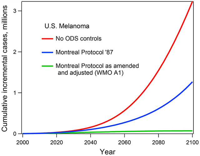
The benefits of the A1 scenario compared with the No Controls and MP’87 scenarios are illustrated in Figure 9a for one health effect and are summarized in Table 4 for all. Under both comparison scenarios, the number of new cases per year would have increased exponentially, with impacts continuing into the next century. Of course, the MP’87 provided some improvement and slowing of the growth of EESC, but it would still have been increasing by 2100. Cohorts born in the second half of this century could have expected high exposures to UV radiation throughout their lifetime, even assuming no worsening of ozone depletion beyond 2100, as shown in Figure 9b. The continued ozone layer degradation under the No Controls and initial Montreal Protocol scenarios highlights the policy importance of the continued strengthening of the Montreal Protocol described in the Introduction. The unabated growth of adverse health effects in the No Controls scenario compared with the more aggressive controlled scenarios (i.e., MP’87 and phaseout accelerated by amendments and adjustments to the Protocol) underlies much of the estimated incremental health benefits in this study.

Figure 9.

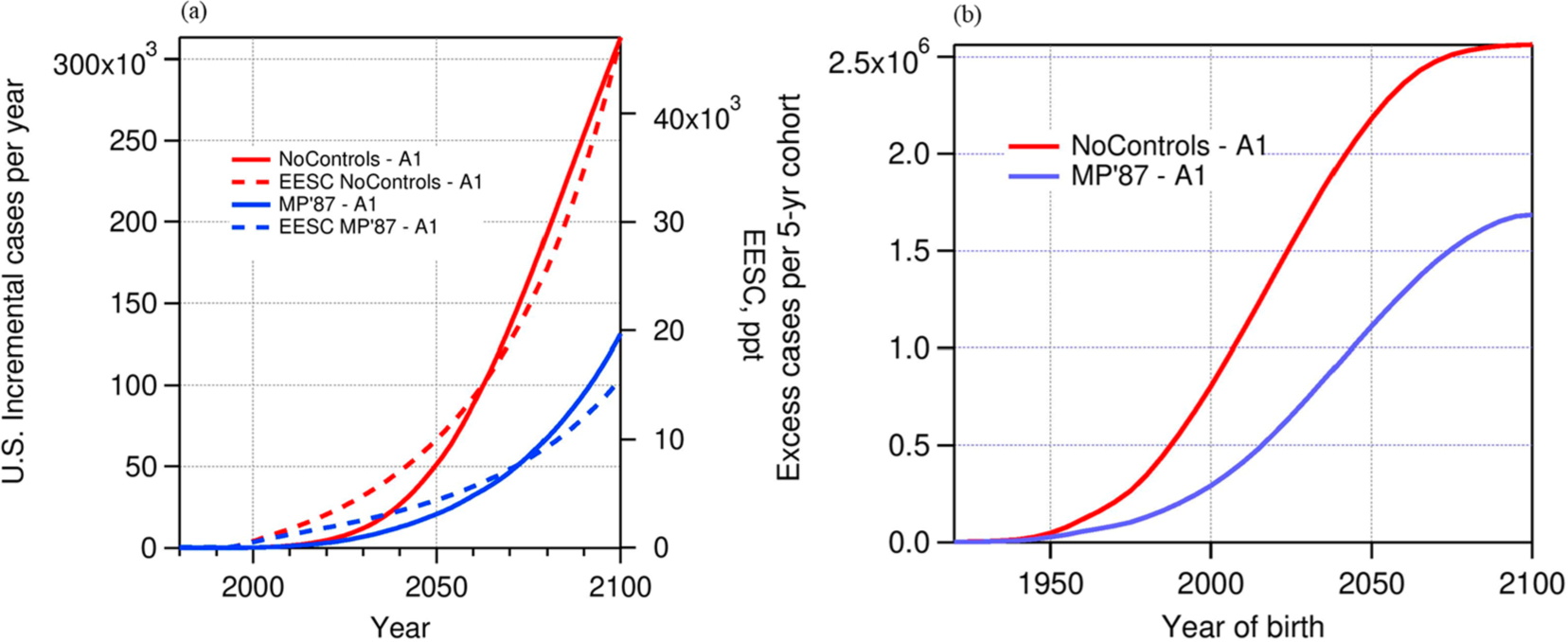
(a) Annual incidence (excess new cases) versus calendar year for white female squamous cell carcinoma incidence for the No Controls and MP’87 scenarios relative to the A1 scenario. (b) Annual incidence (excess new cases) of squamous cell carcinoma among white females versus cohort birth year for the No Controls and MP’87 scenarios relative to the A1 scenario.

With the current value of a life estimated to be around $9–11 million (2020$)⁴⁸ by the EPA, the millions of skin cancer deaths and public healthcare expenditures avoided through the implementation of the Montreal Protocol represent a significant societal and economic benefit.

4. DISCUSSION

4.1. Uncertainty Considerations.

The health effect projections made with the AHEF are subject to a variety of uncertainties. A detailed uncertainty and sensitivity analysis was carried out,³⁰ and its main aspects are summarized here.

Among the atmospheric components, the largest uncertainty arises from the ozone trends (1979–1991) derived from the TOMS satellite-based observations. The TOC trends depend on the latitude and month (see Figure 2), as do their uncertainties. For the annually averaged TOC, McPeters et al.²³ estimated trend uncertainties of at least ±20% (1σ) at subpolar and midlatitudes, increasing sharply in the subtropics, so that ±30% can be considered a conservative overall contribution.

Estimates for EESC have varied considerably in recent assessments^6,12,13 due to improvements in the methods of calculation, in particular, for lifetimes of individual ODSs and their fractional release factors. (See Section 2.2.) A detailed analysis of the uncertainties in EESC was carried out by Velders and Daniel.²⁰ The EESC values are normalized to their 1980 values (see eq 3) so that some common errors cancel, but key uncertainties concern the relative contributions of the various ODSs and the precise timing between emissions and tropospheric mixing ratios. For a scenario very similar to A1, Velders and Daniel²⁰ estimated EESC’s return to 1980 levels by 2048 but with a 2039–2064 confidence interval (95%); for the A1 scenarios, this translates to a range of 300 ppt or about ±7% (1σ) uncertainty in the EESC and 10% for EESC(year)/ EESC(1980).

Other errors related to the atmosphere are much smaller. Errors in the calculation of UV radiation are minor (<5%) for clear skies, but clouds introduce some possible geographic distortions; for example, two locations with the same latitude could experience cloud-related differences in exposures to UV radiation. These differences are already inherent in the baseline incidence and thus have a second-order effect if cloud distributions are assumed to remain unchanged into the future.

The largest uncertainties related to each health effect arise from (a) the choice of action spectrum to calculate the I_bio for the effect of interest and (b) the value of the BAF describing how sensitively each health effect responds to changes in the I_bio. Sensitivity studies using an action spectrum for DNA damage,⁴⁹ which has a higher sensitivity to ozone change compared with the SCUP-h spectrum, led to 40% more melanoma and 80% more keratinocyte mortality.³⁰ Uncertainties in BAFs (Table 3) range from ~30% for skin cancer to ~50% for cataract induction and thus are also an important contribution to the overall uncertainty. However, uncertainties arising from action spectra are not necessarily independent of BAF uncertainties because an action spectrum must be assumed to compute the latitudinal variation in UV radiation that is associated with the incidence data and from which the BAF is derived. This means that as long as the same action spectrum is used for both the original BAF estimation and for estimating the effects of ozone depletion, a partial offset of errors is expected. (See the Supporting Information.)

In summary, the major quantifiable sources of error are from the stratospheric ozone trends, the choice of action spectra, and the estimation of BAFs, for a combined error of 50–70% or a multiplicative factor of ~2. This level of uncertainty is in line with other modeling studies of future health effects due to atmospheric changes, for example, tropospheric ozone.⁴⁹

It should be recognized that there exist many other largely unquantifiable sources of uncertainty. These include uncertainties about the future composition of the atmosphere and how changes in climate will affect ozone, clouds, and aerosols. There is also uncertainty about the present and future distribution of skin types in the U.S. population. Self-reported race to the U.S. Census Bureau does not unambiguously align with the “light-skinned” and “dark-skinned” populations for which BAFs are calculated; including more or fewer ambiguous subpopulations in the “dark-skinned” group leads to estimates of fewer or more cancer health effects, respectively, due to this group’s lower sensitivity to UV-induced skin cancer. A sensitivity analysis with more subpopulations included in the “dark-skinned” group led to results that were 1–8% lower for the present and 11–17% lower in the long term than the skin cancer estimates reported in this study.

Global compliance with modeled policy scenarios is assumed, but demographic and human behavior changes could substantially modify outcomes. Certainly, under the catastrophic scenarios in which UV irradiances are doubled or tripled (see Figure 5), it would seem prudent to alter exposure behaviors. These various uncertainties are not addressed here, as the thrust of our analysis is to estimate the ODS-related effects, other factors (e.g., behavior) being equal.

4.2. Future Considerations.

One facet of understanding the links between changing exposure to UV radiation and disease, and thus what the AHEF model can and cannot explicate, is related to changes in detection and treatment. The AHEF model estimates the induction of disease by UV, but the data it is based on and the statistics to which the model output is compared also depend on the detection and, in the case of mortality, on the treatment of those diseases. Not all cataracts or tumors are identified and recorded, and the rate of detection varies across populations and time.⁵⁰ Therefore, a future increase in induced disease will only lead to an exactly proportional increase in the cases and deaths recorded in medical records if the detection rate is the same. When tumors are identified, differences in the time between tumorigenesis and diagnosis can result in different distributions of tumor invasiveness and metastases, which lead to varying survival rates. Survival rates also vary as a function of treatment methodology and availability.⁵¹ For example, over the past decade, many new treatments have been approved for use in the United States, and from 2013 to 2016, the melanoma mortality decreased by 17.9%, even as the population, average age, and melanoma incidence increased.⁵² The understanding of the progression of skin cancers and of how lesions develop resistance to treatments continues to improve, and additional classes of drugs for treatment of melanoma are under development.

As the ability to detect and treat UV-induced diseases continues to change, the AHEF model can incorporate these changes to remain current with the state of the science. Updated data will affect health estimates in two major ways. First, the percentage of cases induced by UV radiation that are diagnosed, when in the progression of disease those cases are detected, and the treatment of the disease after it is detected are all implicit in the BAFs, with a particular impact on mortality BAFs. The current BAFs for melanoma are based on 1950–1979 health data, and there have been significant developments in detection and treatment since then (although we note that AHEF estimates remain in good agreement with the data through the 2010s (see Table 4)). Second, the effectiveness of the detection and treatment determined the levels of incidence and mortality that underlie the baseline levels associated with no ozone depletion, as only induced disease that was actually diagnosed is represented in historical incidence figures, and the effectiveness of treatment options determined the historical ratios between cases and deaths. Improvements in the detection and treatment may be one driver of the cohort effects seen in Figure 4. To some extent, the effects of changing detection and treatment on the baseline and BAFs may be correlated, and determining incremental effects by subtracting the baseline from scenario levels of disease may reduce the effect of these changes. However, cataracts, keratinocyte cancer, and melanoma all comprise multiple subtypes with different etiologies and correlations with exposure to UV radiation. Therefore, the effects of detection and treatment on the baseline and BAFs will differ. Thus using updated health statistics to recalculate baselines and BAFs is a potential future opportunity to continue the pattern of updates and refinements that the AHEF model has followed.

Future changes in UV radiation are also likely to arise from factors other than stratospheric ozone variations. In one analysis (Bais et al. 2015),⁵¹ future UV levels were evaluated from an ensemble of numerical simulations under the fifth Climate Model Intercomparison Project (CMIP-5)⁵³ using the Representative Concentrations Pathways 4.5 (RCP4.5) emissions scenario. Assuming compliance with the Montreal Protocol, future UV changes at midlatitudes will likely be dominated by aerosols associated with human activities and, to a lesser extent, by changing clouds, whereas in polar regions, changes in reflectivity and stratospheric ozone will be more important.⁵¹ However, the study noted very low confidence in aerosol projections, low confidence for cloud and surface reflections, and good confidence for ozone changes.

5. CONCLUSIONS

The significant health benefits estimated by the AHEF model resulting from decreased ODS emissions under the Montreal Protocol highlight the achievement of the global effort to protect the ozone layer and the importance of efforts to strengthen the Protocol through its amendments and adjustments. In the words of Kofi Annan, the Montreal Protocol has been “perhaps the single most successful international environmental agreement”.⁵⁴ Because the estimated health benefits described in this study assume a continued decrease in ODS emissions, it is also clear that the continuing work of implementing the phaseout called for under the Montreal Protocol plays an important role in protecting people’s health. The cross-disciplinary connections provided by the AHEF model are a unique contribution to quantifying the impact of the global and national policies precipitated by these international efforts.

REFERENCES

- (1).Molina MJ; Rowland FS Stratospheric Sink for Chlorofluoromethanes: Chlorine Atom-Catalysed Destruction of Ozone. Nature 1974, 249, 810–812. [Google Scholar]
- (2).Farman JC; Gardiner BG; Shanklin JD Large losses of total ozone in Antarctica reveal seasonal ClOx/NOx interaction. Nature 1985, 315 (6016), 207–210. [Google Scholar]
- (3).Solomon S; Garcia RR; Rowland FS; Wuebbles DJ On the depletion of Antarctic ozone. Nature 1986, 321 (6072), 755–758. [Google Scholar]
- (4).Solomon S Stratospheric ozone depletion: A review of concepts and history. Rev. Geophys 1999, 37 (3), 275–316. [Google Scholar]
- (5).Gleason JF; Bhartia PK; Herman JR; McPeters R; Newman P; Stolarski RS; Flynn L; Labow G; Larko D; Seftor C; Wellemeyer C; Komhyr WD; Miller AJ; Planet W Record low global ozone in 1992. Science 1993, 260 (5107), 523–526. [DOI] [PubMed] [Google Scholar]
- (6).World Meteorological Organization (WMO). Scientific Assessment of Ozone Depletion: 2018; Global Ozone Research and Monitoring Project – Report No. 58; 2018.
- (7).Environmental Effects Assessment Panel (EEAP). Environmental Effects and Interactions of Stratospheric Ozone Depletion, UV Radiation, and Climate Change; 2018Assessment Report; United Nations Environment Programme (UNEP): Nairobi, Kenya, 2019. [Google Scholar]
- (8).American Cancer Society. Melanoma of the Skin; Cancer Statistics Center, 2021. [Google Scholar]
- (9).Madronich S; de Gruijl FR Skin cancer and UV radiation. Nature 1993, 366 (6450), 23. [DOI] [PubMed] [Google Scholar]
- (10).Slaper H; Velders GJ; Daniel JS; de Gruijl FR; van der Leun JC Estimates of ozone depletion and skin cancer incidence to examine the Vienna Convention achievements. Nature 1996, 384 (6606), 256–258. [DOI] [PubMed] [Google Scholar]
- (11).van Dijk A; Slaper H; den Outer PN; Morgenstern O; Braesicke P; Pyle JA; Garny H; Stenke A; Dameris M; Kazantzidis A; Tourpali K; Bais AF Skin cancer risks avoided by the Montreal Protocol – worldwide modeling integratind coupled climate chemistry models with a risk model for UV. Photochem. Photobiol 2013, 89 (1), 234–246. [DOI] [PubMed] [Google Scholar]
- (12).World Meteorological Organization (WMO). Scientific Assessment of Ozone Depletion: 2010; Global Ozone Research and Monitoring Project – Report No. 52; Geneva, Switzerland, 2011. [Google Scholar]
- (13).World Meteorological Organization (WMO). Scientific Assessment of Ozone Depletion: 2014; Global Ozone Research and Monitoring Project – Report No. 56; Geneva, Switzerland, 2014. [Google Scholar]
- (14).The ALE/GAGE/AGAGE Network (DB 1001); Carbon Dioxide Information Analysis Center: Berkeley, CA, 2016. [Google Scholar]
- (15).Prinn R; Weiss R; Arduini J; Arnold T; DeWitt H; Fraser P; Ganesan A; Gasore J; Harth C; Hermansen O; Kim J; Krummel P; Li S; Loh Z; Lunder C; Maione M; Manning A; Miller B; Mitrevski B; Mühle J; O’Doherty S; Park S; Reimann S; Rigby M; Saito T; Salameh P; Schmidt R; Simmonds P; Steele L; Vollmer M; Wang HJ; Yao B; Yokouchi Y; Young D; Zhou L History of Chemically and Radiatively Important Atmospheric Gases from the Advanced Global Atmospheric Gases Experiment (AGAGE); Carbon Dioxide Information Analysis Center (CDIAC), Oak Ridge National Laboratory (ORNL): Oak Ridge, TN, 2011. DOI: 10.3334/CDIAC/ATG.DB1001. [DOI] [Google Scholar]
- (16).The Alternative Fluorocarbons Environmental Acceptability Study (AFEAS). Advanced Global Atmospheric Gases Experiment. 2020. [Google Scholar]
- (17).Technology and Economic Assessment Panel (TEAP). Report of the Technology and Economic Assessment Panel – May 2008; United Nations Environment Programme: Nairobi, Kenya, 2008. [Google Scholar]
- (18).Velders GJM; Andersen SO; Daniel JS; Fahey DW; McFarland M The Importance of the Montreal Protocol in Protecting Climate. Proc. Natl. Acad. Sci. U. S. A 2007, 104 (42), 4814–4819. [DOI] [PMC free article] [PubMed] [Google Scholar]
- (19).Newman PA; Daniel JS; Waugh DW; Nash ER A new formulation of equivalent effective stratospheric chlorine (EESC). Atmos. Chem. Phys 2007, 7 (17), 4537–4552. [Google Scholar]
- (20).Velders GJM; Daniel JS Uncertainty analysis of projections of ozone-depleting substances: mixing ratios, EESC, ODPs, and GWPs. Atmos. Chem. Phys 2014, 14 (6), 2757–2776. [Google Scholar]
- (21).Daniel JS; Solomon S; Albritton DL On the evaluation of halocarbon radiative forcing and global warming potentials. J. Geophys. Res.: Atmos 1995, 100 (D1), 1271–1285. [Google Scholar]
- (22).McPeters RD; Bharita PK; Herman JR; Oaks A Nimbus-7 Total Ozone Mapping Spectrometer (TOMS) Data Products User’s Guide; National Aeronautics and Space Administration, Scientific and Technical Information Branch, 1996. [Google Scholar]
- (23).McPeters RD; Hollandsworth SM; Flynn LE; Herman JR; Seftor CJ Long-term ozone tends derived from 16-year combined Nimbus 7/Meteor 3 TOMS Version 7 Record. Geophys. Res. Lett 1996, 23, 3699–3702. [Google Scholar]
- (24).de Gruijl FR; Sterenborg HJCM; Forbes PD; Davies RE; Cole C; Kelfkens G; van Weelden H; Slaper H; van der Leun JC Wavelength dependence of skin cancer induction by ultraviolet irradiation of albino hairless mice. Cancer Res 1993, 53, 53–60. [PubMed] [Google Scholar]
- (25).Oriowo OM; Cullen AP; Chou BR; Sivak JG Action spectrum recovery for in vitro UV-induced cataract using whole lenses. Invest. Ophthalmol. Visual Sci 2001, 42, 2596–2602. [PubMed] [Google Scholar]
- (26).Micheletti MI; Piacentini RD; Madronich S Sensitivity of Biologically Active UV Radiation to Stratospheric Ozone Changes: Effects of Action Spectrum Shape and Wavelength Range. Photochem. Photobiol 2003, 78 (5), 456–461. [DOI] [PubMed] [Google Scholar]
- (27).Lee-Taylor J; Madronich S Climatology of UV-A, UV-B, and Erythemal Radiation at the Earth’s Surface, 1979–2000; NCAR Technical Note TN-474-STR; 2007. DOI: 10.5065/D62J68SZ. [DOI] [Google Scholar]
- (28).Madronich S Photodissociation in the Atmosphere 1. Actinic Flux and the Effects of Ground Reflections and Clouds. J. Geophys. Res 1987, 92 (D8), 9740–9752. [Google Scholar]
- (29).Pitcher HM; Longstreth JD Melanoma mortality and exposure to ultraviolet radiation: An empirical relationship. Environ. Int 1991, 17, 7–21. [Google Scholar]
- (30).U.S. Environmental Protection Agency. Human Health Benefits of Stratospheric Ozone Protection. 2006.
- (31).de Gruijl FR; Forbes PD UV-induced skin cancer in a hairless mouse model. BioEssays 1995, 17 (7), 651–660. [DOI] [PubMed] [Google Scholar]
- (32).West SK; Longstreth JD; Munoz BE; Pitcher HM; Duncan DD Model of Risk of Cortical Cataract in the US Population with Exposure to Increased Ultraviolet Radiation due to Stratospheric Ozone Depletion. Am. J. Epidemiol 2005, 162, 1080–1088. [DOI] [PubMed] [Google Scholar]
- (33).U.S. Environmental Protection Agency. Protecting the Ozone Layer Protects Eyesight: A Report on Cataract Incidence in the United States Using the AHEF Model. 2010.
- (34).Scotto J; Pitcher H; Lee JAH Indications of future decreasing trends in skin-melaonma mortality among whites in the United States. Int. J. Cancer 1991, 49, 490–853. [DOI] [PubMed] [Google Scholar]
- (35).Ries LAG; Kosary CL; Hankey BF; Miller BA; Edwards BK SEER Cancer Statistics Review, 1973–1996; National Cancer Institute: Bethesda, MD, 1999. [Google Scholar]
- (36).U.S. Environmental Protection Agency (EPA). Regulatory Impact Analysis: Protection of Stratospheric Ozone. 1987.
- (37).Fears TR; Scotto J Estimating increases in skin cancer morbidity due to increases in ultraviolet radiation exposure. Cancer Invest 1983, 1, 119–126. [DOI] [PubMed] [Google Scholar]
- (38).Scotto J; Fears TR; Fraumeni JF Jr. Incidence of Nonmelanoma Skin Cancer in the United States; U.S. Department of Health and Human Services: Bethesda, MD, 1983. [Google Scholar]
- (39).Congdon N; Vingerling JR; Klein BEK; West S; Friedman DS; Kempen J; O’Colmain B; Wu SY; Taylor HR; Wang JJ Prevalence of cataract and pseudophakia/aphakia among adults in the United States. Arch. Ophthalmol 2004, 122, 487–494. [DOI] [PubMed] [Google Scholar]
- (40).U.S. Department of Health and Human Services (DHHS). The Surgeon General’s Call to Action to Prevent Skin Cancer; Office of the Surgeon General: Washington, DC, 2014. [PubMed] [Google Scholar]
- (41).Institute for Health Metrics and Evaluations (IHME). Global Health Data Exchange: Global Burden of Disease Results Tool. 2020.
- (42).West SK; Duncan DD; Munoz B; Rubin GS; Fried LP; Bandeen-Roche K; Schein OD Sunlight Exposure and Risk of Lens Opacities in a Population-Based Study. The Salisbury Eye Evaluation Project. JAMA 1998, 280 (8), 714–718. [DOI] [PubMed] [Google Scholar]
- (43).U.S. Census Bureau. Intercensal County Estimates by Age, Sex, Race: 1980–1989. 2016.
- (44).U.S. Census Bureau. Intercensal Estimates of the Resident Population by Five-Year Age Groups, Sex, Race, and Hispanic Origin for Counties: April 1, 2000 to July 1, 2010. 2016.
- (45).U.S. Census Bureau. State and County Intercensal Datasets: 1990–2000. 2017.
- (46).U.S. Census Bureau. Annual County Resident Population Estimates by Age, Sex, Race, and Hispanic Origin: April 1, 2010 to July 1, 2018. 2019.
- (47).U.S. Census Bureau. 2018 National Population Projections Tables: Race and Hispanic Origin by Age Group. 2019.
- (48).U.S. Environment Protection Agency (EPA). Guidelines for Preparing Economic Analyses. 2010.
- (49).Kim Y-M; Zhou Y; Gao Y; Fu JS; Johnson BA; Huang C; Liu Y Spatially resolved estimation of ozone-related mortality in the United States under two representative concertation pathways (RCPs_ and their uncertainty. Clim. Change 2015, 128, 71–84. [DOI] [PMC free article] [PubMed] [Google Scholar]
- (50).Leachman SA; Cassidy PB; Chen SC; Curiel C; Geller A; Gareau D; Pellacani G; Grichnik JM; Malvehy J; North J; Jacques SL; Petrie T; Puig S; Swetter SM; Tofte S; Weinstock MA Methods of Melanoma Detection. Cancer Treat. Res 2016, 167, 51–105. [DOI] [PubMed] [Google Scholar]
- (51).Bais AF; McKenzie RL; Bernhard G; Aucamp PJ; Ilyas M; Madronich S; Tourpali K Ozone depletion and climate change impacts on UV radiation. Photochem. Photobiol. Sci 2015, 14 (1), 19–52. [DOI] [PubMed] [Google Scholar]
- (52).Berk-Krauss J; Stein JA; Weber J; Polsky D; Geller AC New Systematic Therapies and Trends in Cutaneous Melanoma Deaths Among US Whites, 1986–2016. Am. J. Public Health 2020, 110 (5), 731–733. [DOI] [PMC free article] [PubMed] [Google Scholar]
- (53).Eyring V; Arblaster JM; Cionni I; Sedlacek J; Perlwitz J; Young PJ; Bekki S; Bergmann D; Cameron-Smith P; Collins WJ; Faluvegi G; Gottschaldt K-D; Horowitz LW; Kinnison DE; Lamarque J-F; Marsh DR; Saint-Martin D; Shindell DT; Sudo K; Szopa S; Watanabe S Long-term ozone changes and associated climate impacts in CMIP5 simulations. J. Geophys. Res.: Atmos 2013, 118 (10), 5029–5060. [Google Scholar]
- (54).Tolba M Green Giant. The Economist (London, England), March31, 2015. https://www.economist.com/science-and-technology/2016/03/31/green-giant (accessed 2021-07-06). [Google Scholar]
Associated Data
This section collects any data citations, data availability statements, or supplementary materials included in this article.