A model based on cellular automata for investigating the impact of lockdown, migration and vaccination on COVID-19 dynamics

Abstract

Background and Objective:COVID-19 pandemic continues unabated due to the rapid spread of new mutant strains of the virus. Decentralized cluster containment is an efficient approach to manage the pandemic in the long term, without straining the healthcare system and economy.

In this study, the objective is to forecast the peak and duration of COVID-19 spread in a cluster under different conditions, using a probabilistic cellular automata configuration designed to include the observed characteristics of the pandemic with appropriate neighbourhood schemes and transition rules.

Methods: The cellular automata, initially configured to have only susceptible and exposed states, enlarges and evolves in discrete time steps to different infection states of the COVID-19 pandemic. The transition rules take into account the probability and proximity of contact between infected hosts and susceptible individuals. A transmittable and transition neighbourhoods are defined to identify the most probable individuals infected from a single host in a time step.

Results: The model with novel neighbourhood schemes and transition rules reproduce the macroscopic behaviour of infection and recovery observed in pandemics. The temporal evolution of the pandemic trajectory is sensitive to lattice size, range, latent and recovery periods but has constraints in capturing the changes in the infectious period. A study of lockdown and migration scenarios shows strict social isolation is crucial in controlling the pandemic. The simulations also indicate that earlier vaccination with a higher capacity and rate is essential to mitigate the pandemic. A comparison of simulated and actual data shows a good match.

Conclusions: The study concludes that social isolation during movement and interaction of people can limit the spread of new infections. Vaccinating a large proportion of the population reduces new cases in subsequent waves of the pandemic. The model and algorithm with real-world data as input can quickly forecast the trajectory of the pandemic, for effective response in cluster containment.

1. Introduction

The world is facing an unprecedented challenge. The challenge, Coronavirus Disease-2019 (COVID-19), caused by Severe Acute Respiratory Syndrome Coronavirus 2 (SARS-CoV-2), first identified in Wuhan, China, in December 2019 is still spreading havoc. The World Health Organization (WHO) declared COVID-19 a global pandemic on 11 March 2020 [1], and this infectious disease is now showing further surges due to the proliferation of mutant strains of the virus.

Stringent implementation of healthcare advisories from WHO, strategies such as national lockdowns [2], [3] and effective interventions by Governments in testing, isolating and treating the infected aided to control the spread of the virus in its first wave [4], [5], [6]. Nevertheless, the viral pandemic affected human life and the global economy in an adverse manner [7]. The relentless efforts of the scientific community in developing vaccines for the disease is finally a success and vaccination programs are taking place all over the world [8], [9].

Strategic planning and efficient deployment of resources is crucial in controlling this pandemic without overwhelming the healthcare system or further affecting the economy [10], [11]. This requires information on future demands of medical equipment and additional infrastructure that may be needed [12]. Computational models can provide valuable insights in this regard by forecasting the growth trends of the pandemic under different circumstances [13], [14], [15]. Possibility for repeated and cost-effective parametric studies in a virtual environment, flexibility to include and adapt to real-time data and simulation in a short duration, are some of the other advantages of modeling.

Mathematical modeling of infectious diseases is a mature area with many well-known methods [16], [17] and there have been several efforts in modeling COVID-19 too [18], [19]. Simple deterministic compartment models are a popular approach in simulating evolving pandemics [20]. In this approach, the entire population is divided into distinct compartments at a particular instant of time, based on infection status. The simplest compartment model is $SIR$ model, which consists of three states, $S$ for susceptible individuals, $I$ for infected and $R$ for recovered individuals [21]. Additional compartments can be added to the model to simulate other infection states observed in a pandemic. These are either formulated and computed as ordinary differential equations or methods such as Cellular Automata (CA) approach are used for the simulation [22], [23], [24].

COVID-19 exhibits different transmission characteristics compared to other infectious diseases [25] and mathematical models have been successful in identifying relevant parameters and reproducing observed disease dynamics [26], [27], [28], [29], [30]. CA configurations, with their flexibility for defining heterogeneous states and local rules for state transitions based on neighbourhood information, are ideal for simulating epidemics [31], [32], [33]. This method has been successfully used for predicting long term behaviour of COVID-19 [34] and also to understand the effect of lockdown measures in a region [35], [36].

In a recent study, Ghosh and Bhattacharya [37], used Probabilistic Cellular Automata (PCA) with simulation parameters optimized using a sequential genetic algorithm to forecast COVID-19 dynamics. This combination is shown to accurately estimate the time trajectory of COVID-19 when physically meaningful parameters are used. In this CA configuration, the initial population with different disease states are distributed in a 2D lattice of fixed size. In another work, the same authors incorporated factors like population density, testing efficiency and movement restriction into a PCA model through appropriate probabilities to explain the variability of disease dynamics observed in different countries [38].

In another important work, Schimit [39], studied the impact of social isolation on dynamics of COVID-19 using PCA and ordinary differential equations. The model consists of eight disease states and fifteen parameters and uses an extended neighbourhood to establish random contact networks between cells. Each state transition is based on either probabilities or pre-defined periods to account for the uncertainties in COVID-19 propagation. The results suggest that maintaining social isolation is crucial to keep the pandemic spread under control and to avoid the overwhelming of the healthcare system. The model is formulated for a country, with a fixed lattice size of the order of 210 million and the simulation is reported to take over a week to complete.

A spatiotemporal epidemiological forecast model for short and long term local infection risk predictions for smaller regions such as counties is proposed by Zhou et al. [40]. The work shows that, by using local information in the model through a CA which enables interconnectivity and regional variations, the prediction error is significantly reduced compared to that for a larger space. Dai et al. [41] predict the spread patterns of COVID-19 in cities using a CA model that incorporates factors such as sex ratio, age, immunity and various disease characteristics. The movement of the population is simulated by defining moving proportion and a maximum moving step length in a fixed lattice size with occupied and empty cells.

Decentralised response through cluster containment or regional lockdowns is an effective approach to manage the pandemic in a short period [42]. Real-time surveillance of small geographical clusters called micro-containment zones enables error-free data collection and analysis, followed by rapid decision making and interventions with minimum disruption to the overall economy. Local administration can mobilise their resources to support the community during the containment and also to implement the find, test, trace, isolate and support system [4], successfully carried out to control the spread of the pandemic in its first wave. Additionally, in cluster containment, the size of the susceptible population, which is a crucial parameter in determining the spread of the pandemic [12] is small and can be easily monitored.

The computational model in the present work is developed based on the idea of monitoring a susceptible population in a cluster to mitigate the pandemic. The susceptible population can be people in a geographical region, or a subgroup in the region identified through the process of contact tracing and kept in quarantine, or people in a particular age group or gender [43]. The size of the susceptible population is not constant but can change during the spread of the pandemic or migration of people. In the literature, most studies on modelling COVID-19 using CA have used a fixed lattice size with human-occupied and empty cells. We propose to use a variable size lattice, initially with only susceptible and infected cells in it, which increases in size to accommodate the incoming susceptible or infectious population. From the simulation perspective, concentrating on the susceptible population eliminates empty cells, keeps the size of the lattice small, computational time and memory requirements to a minimum and model varialbes to a few. Hence, in this work, we develop a PCA model, by defining novel neighbourhood schemes and transition rules to include COVID-19 transmission and propagation characteristics and investigate the disease dynamics in a variable susceptible population under different conditions.

The next section describes the model and algorithm in detail. Important model parameters are identified from a sensitivity analysis in the third section. The fourth section discusses the effect of lockdown, migration and vaccination on COVID-19 dynamics and presents a validation of the model.

2. Methods: probabilistic cellular automata

Cellular automata are discrete dynamical systems with a finite number of identical cells [33]. The information of interest is stored in each cell and is called the state of the cell. There could be a finite set of distinct states depending on the phenomena being investigated. The states of the cells are updated simultaneously in discrete time steps, according to a pre-defined transition function [44]. The evolution of the state of a particular cell depends on its state and the states of its local neighbourhood of cells. The transition functions may be deterministic or probabilistic and are uniform in space and time. These are either given by analytical functions or as a set of transition rules [45]. The local transition functions are formulated such that, they replicate the physical behaviour of the system being studied. The cellular automata $\mathbb{C}$, thus can be represented as a tuple of four elements $\mathbb{C}=(\mathcal{L},\mathcal{A},\mathcal{N},\mathcal{F})$, namely lattice $\mathcal{L}$, state $\mathcal{A}$, neighbourhood $\mathcal{N}$ and transition function $\mathcal{F}$ [15].

The cells of a CA can be represented as uniformly arranged elements in a two-dimensional space ${\mathbb{Z}}^2$. Mathematically the lattice $\mathcal{L}=\{x_{ij},1⩽i⩽m,1⩽j⩽n\}$, where $\mathcal{L}\subset {\mathbb{Z}}^2$, is a two dimensional array of $m\times n$ cells, and $x_{ij}\in \mathcal{L}$ for the cell $x$ with indices $i$ and $j$. A two-dimensional square lattice with $m=n$ is used in the present work. The detailed formulation of $\mathcal{A},\mathcal{N}$ and $\mathcal{F}$ are described in the following sections.

2.1. Cellular automata configuration for Covid-19 simulation

In the present CA configuration, a cell represents a person, and various stages of the infection life-cycle undergone by the person, from susceptible to recovery or vaccinated, are represented by the state of that cell. The probable state of a cell is an element of a finite and ordered state set defined as $\mathcal{A}=\{S,E,L,I,T,R,V\}$. Here the epidemiological states are represented by $S$ the susceptible (potential) state, $E$ exposed (infected) state, $L$ latent state, $I$ infectious state, $T$ treatment state, $R$ recovered (removed) state and $V$ the vaccinated state.

In the computer code, a particular state is identified by assigning a single or range of numerical values called state values to it. The state values, denoted by $v$, starts with 0 and extends to a user-defined upper limit $t_R$, which represents the average time for recovery. Every state $\mathfrak{a}\in \mathcal{A}$, is assigned a state value $v$ as a function of time by $g\left(t\right):\mathcal{V}\to \mathcal{A}$ where $\mathcal{V}=\{v,0⩽v⩽t_R\}$. The values 0 and 1 represents susceptible and exposed states respectively. The details of other states in $\mathcal{A}$ and corresponding numerical value set $\mathcal{V}$ used to represent these states are given in Table 1 . The values of latent, infectious and treatment periods are flexible and can be decided based on scientific studies.

Table 1.

Cellular automata states and assigned numerical values.

CA State $\mathfrak{a}$	Notation of $\mathfrak{a}$	State value $v$
	($\mathfrak{a}\in \mathcal{A}$)	($v\in \mathcal{V}$)
Susceptible (potential)	$S$	0
Exposed (infected)	$E$	1
Latent	$L$	2, 3
Infectious	$I$	4 to 8
Treatment	$T$	9 to 14
Recovered (Removed)	$R$	$t_R=15$
Vaccinated	$V$	$t_R+1=16$

A susceptible state $v=0$ will become infected only as per local transition rules to be defined shortly. All other state values are sequentially updated in each time step by $v=v+1$. This updating represents the movement from the exposed state to the recovered state through different stages of infection. The discrete-time step used in the simulation is $1day$. Hence, the state value $v$ of a cell also indicates days passed after that cell became infected. The updating of state value is stopped when $v=t_R$, the recovered state. It is assumed that the vaccinated people are immune to infection and all infected people are recovered in due course of time.

A cell, with a particular state assigned to it at time $t$, is denoted by $x_{ij}^t$. There will be a corresponding global state configuration of CA denoted by ${\mathcal{L}}^t=\left\{x_{ij}^t\right\}$, which is an array of states of all cells at time $t$. The most probable $S$ state cells, in ${\mathcal{L}}^t$, to which virus transmission can happen in a particular time step are identified by the procedure described further.

2.2. Transition and transmittable neighbourhoods

The neighbourhood of a cell is a set of its surrounding cells whose states influence the evolution of that cell. The state $x_{ij}^{t+1}$ of a cell at time $t+1$ is a function of its own state and that of its neighbourhood cells $\mathcal{N}\subset {\mathbb{Z}}^2$ at time $t$. The number of cells in the neighbourhood can be decided depending on the phenomena being simulated.

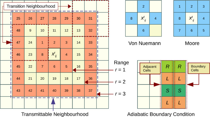
Two of the commonly used neighbourhood schemes in cellular automata computations are Von Neumann and Moore neighbourhoods of range $r=1$ as shown in Fig. 1 . In the Von Neumann scheme, the states of $x_{ij}$ and its four adjacent cells excluding the four diagonal cells constitute the neighbourhood; whereas in the Moore scheme, states of $x_{ij}$ and all eight surrounding cells forms the neighbourhood.

Fig. 1.

Neighbourhood schemes and boundary conditions.

For a cell $x_{ij}$, the Moore neighbourhood of range $r$ is defined as a finite set ${\mathcal{N}}_{ij}^r=\{(k,l)\in {\mathbb{Z}}^2,|k-i|\le r\text{and}|l-j|\le r\}$, where $(k,l)$ represents the indices of neighbourhood cells. Range $r$ indicates the number of adjacent layers of cells that are included in the neighbourhood, such that the cardinality of ${\mathcal{N}}_{ij}^r$ is $4r(r+1)$. A neighbourhood configuration ${\mathcal{N}}_{ij}^{rt}$ contains information on states of each cell in the neighbourhood at time $t$.

In the model, to simulate the local interactions of Covid-19 propagation, two types of neighbourhoods are defined. The first one is an extended neighbourhood, called a transmittable neighbourhood, defined around an infectious cell and the second is the transition neighbourhood, defined around a susceptible cell. The transmittable neighbourhood identifies all potential cells for virus transmission, and the transition neighbourhood decides whether that transmission will happen or not.

An infectious cell at time $t$ can transmit the virus to many potential cells in its transmittable neighbourhood, that become infected at time $t+1$. The transition of a potential cell from $x_{ij}^t=S$ to $x_{ij}^{t+1}=E$ will but depend on states of cells in its transition neighbourhood. A Moore scheme of $r=1$ around potential cell $x_{ij}^t=S$ is taken as the transition neigbhourhood and a Moore scheme of $r=3$ around the cell $x_{ij}^t=I$ is taken as the transmittable neighbourhood. The cardinality of ${\mathcal{N}}_{ij}^1=8$, ${\mathcal{N}}_{ij}^2=24$ and ${\mathcal{N}}_{ij}^3=48$ (Fig. 1). Defining the transmittable neighbourhood as an extended Moore scheme of 48 cells increases the chances of finding potential cells around a host, which meets various constraints for virus transmission compared to a traditional Moore scheme of 8 cells. This enables the reproduction of an observed infection rate, especially during lockdown conditions.

Additionally, the transmittable neighbourhood of range $r=3$ brings in the following interactions of importance observed in Covid-19 propagation in to the model. ${\mathcal{N}}_{ij}^1$ represents the primary contacts and ${\mathcal{N}}_{ij}^2$ represents the secondary contacts to infectious person. ${\mathcal{N}}_{ij}^3$ takes into account the exposure due to the movement of people in the locality. All the 48 cells in the transmittable neighbourhood are examined to identify potential $S$ state cells which may get infected in a particular time step. The model algorithm will scan the extended neighbourhood only if potential cells are not found in lower ranges.

2.3. Virus transmission in transmittable neighbourhood

Transmission of the SARS-CoV-2 virus is reported to happen when there is direct, indirect or close contact between infected persons and others. Testing, identifying and isolating infected people is an important step in breaking the chain of virus transmission [46]. The computational model thus should include parameters accounting for local interaction of people for realistic forecasting of the disease dynamics [25], [47]. Two parameters, namely, social isolation factor for the locality and social isolation factor for the individual, are defined to account for the possibility of movement and contact of people. These factors represent the probability of virus transmission and bring in the stochasticity of COVID-19 dynamics into the model.

The imposed restrictions to movement in a region is represented by social isolation factor for locality ${\lambda }_l$, with ${\lambda }_l=0$ for unrestricted movement and ${\lambda }_l=1$ for total restriction. The value of ${\lambda }_l$ is the same for the entire lattice and is kept constant for a particular duration of time such as the lockdown period. The movement of an individual in a region depends on the receptiveness of restrictions and regulations by the individual. The social isolation factor for the individual ${\lambda }_p$, which is unique and time-dependent accounts for this. The value of ${\lambda }_p$ is randomly generated in the time step and has a range of 0 to 1, with 0 representing total compliance and 1 representing no compliance to restrictions. For an infected individual, the condition ${\lambda }_p<{\lambda }_l$, indicates that the person complies with imposed restrictions and virus transmission will not happen from that individual. Whereas the condition ${\lambda }_p\ge {\lambda }_l$, indicates the possibility of contact between an infected individual and susceptible people, and a high chance of transmission.

If the condition ${\lambda }_p\ge {\lambda }_l$ is satisfied for an infected cell, then the procedure of identifying exposed cells in its neighbourhood involves a two-step process. Both these steps are sequentially executed in each time step. In the first step, the transmittable neighbourhood of the infected cell is examined and a finite set $\left\{C_{ij}\right\}$ with all potential $S$ state cells is created. The elements of the set are a tuple, $(i,j,{\sum }_1^{8}v)\in \left\{C_{ij}\right\}$, which contains indices $i,j$ of each $S$ state cell and a sum of state values of its transition neighbourhood ${\sum }_1^{8}v$. The sum of state values is an indication of the proximity and duration of local interaction between potential and all infected individuals in its transition neighbourhood. $\left\{C_{ij}\right\}$ can be an empty set or can have a maximum cardinality of $4r(r+1)$ in time $t$. An empty set results when no susceptible cells are available in the transmittable neighbourhood. This is the second condition, after ${\lambda }_p<{\lambda }_l$, that leads to a stochastic outcome of the model.

In the second step, $R_t$ number of cells in $\left\{C_{ij}\right\}$ are marked as infected by assigning $v=1$, starting from the cell with the highest value of ${\sum }_1^{8}v$ and proceeding in descending order. The number $R_t$ represents the maximum number of transmission from a single host per time step. The value of $R_t$ can be kept as constant or randomly selected from a set of numbers in each time step. Even though $R_t$ could range from 1 to cardinality of $\left\{C_{ij}\right\}$, selecting a higher value will result in a sudden and unrealistic spread of infection in few time steps. Hence, in the present study a constant value of $R_t=2$ is used. It may be noted that $R_t$ is not the same as the basic reproduction number $R_o$ which represents the average number of secondary infections caused by an infected individual introduced to a susceptible population [34], [48].

2.4. Transition rules and boundary conditions

The global state configuration ${\mathcal{L}}^t$ of the CA is updated in discrete time steps as a sequence of mappings $\mathcal{F}:{\mathcal{L}}^t\to \mathfrak{a},\mathfrak{a}\in \mathcal{A}$, where $\mathcal{F}$ represents the local transition function. The transition rules can be formulated as follows,

• •A cell in an infectious state infects a maximum of $R_t$ susceptible cells in its transmittable neighbourhood when social isolation factor ${\lambda }_p\ge {\lambda }_l$.
• •The $R_t$ number of susceptible cells are identified in decreasing order of their sum of state values.
• •The value of any state other than susceptible is updated sequentially in each time step with $v=v+1$ until $v=t_R$.

In terms of assigned state values $v$, the transition rules can be written as Eq. (1).

$$\begin{array}{cc}\mathcal{F}\hfill & :{\mathcal{L}}^t\to v,v\in \mathcal{V}\hfill \\ v\left(x_{ij}^{t+1}\right)\hfill & =1\text{for}v\left(x_{ij}^t\right)=0\text{if}{x}_{ij}^t\in \left\{C_{ij}^s\right\}\hfill \\ v\left(x_{ij}^{t+1}\right)\hfill & =v\left(x_{ij}^t\right)+1\text{for}0<v\left(x_{ij}^t\right)<t_R\hfill \end{array}$$ (1)

Here, $\left\{C_{ij}^s\right\}\subset \left\{C_{ij}\right\}$ has $R_t$ number of elements with maximum values of ${\sum }_1^{8}v$. It may be noted that only the transition from $S$ to $E$ state takes place as per the procedure explained in Section 2.3. All other mappings $f_{\mathfrak{a}}^{t+1}\left(x_{ij}^t\right),\mathfrak{a}\in \mathcal{A}\setminus E$ progresses in time as mapping to the sequence of states in $\mathcal{A}$, for the duration considered for simulation as $f_{\mathfrak{a}}^{\tau }\left(x_{ij}^t\right),0⩽\tau ⩽(t-1)$.

The initial configuration of the CA consists of only susceptible and infected states i.e., at time $t=0$, ${\mathcal{L}}^0=\{S,E\}$. The state values of all lattice cells are assigned $v=0$, except the infected cells which are assigned a state value of $v=1$. The infected states are randomly assigned in the lattice. An adiabatic boundary condition, in which the boundary cells of the lattice are mapped with their adjacent cell states (Fig. 1), is used in the simulation to handle evolution at lattice boundaries. The mapping can be mathematically represented as Eq. (2).

$$\begin{array}{ccc}{x}_{1j}=x_{2j},\hfill & x_{mj}=x_{(m-1)j},\hfill & j=1\cdots n\hfill \\ x_{i1}=x_{i2},\hfill & x_{in}=x_{i(n-1)},\hfill & i=1\cdots m\hfill \end{array}$$ (2)

This boundary condition is applied and boundary cells are updated in each time step after lattice computations are over. The supplementary file describes the model algorithm in detail.. A computer code is written in Python programming language based on this algorithm. The simulations and analysis are carried out on a computer with AMD Ryzen™3 2200U processor with Radeon™Vega 3 Graphics card and 4 GB RAM.

3. Sensitivity analysis of model parameters

The probabilistic cellular automata model presented above is tested with a fixed susceptible population to see if the model can reproduce the macroscopic behaviour of a pandemic propagation. It is assumed that the entire susceptible population is infected and recovered in due course. Further, a parametric study assesses the qualitative response of the model to changes in input parameters. Table 2 shows the details of parameters used in the simulations.

Table 2.

Model parameters used in simulations.

Parameter	Notation	Value
Discrete time step	$t$	1 day
Range of neighbourhood	$r$	1,2,3
Maximum transmission	$R_t$	2
Lattice dimension (m = n)	m	100, 150, 200
Initial infected	$I$	1
Initial recovered	$R$	0 people
Latent period	$L_p$	1 - 4 days
Infectious period	$I_p$	3 - 9 days
Recovery time	$t_R$	7, 14, 21 days
Social isolation factor, locality	${\lambda }_l$	0
Social isolation factor, person	${\lambda }_p$	Random (0,1)

3.1. Time trajectory of COVID-19 propagation

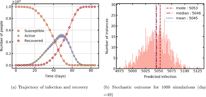
The simulation is initiated with one infected cell placed at the center of the lattice and the temporal evolution of the PCA is shown in Fig. 2 a. The susceptible population decreases, the recovered population increases, and the active infections (states $E,L,I,T$) exhibit growth and decline in time. The time taken for 1000 repeated simulations for statistical analysis is 156 min. The rate of infection increases with time, as the percentage of infected population increases and further accelerates the spread in the susceptible population. The recovered cases gradually increase after the specified recovery time and surpass the active cases with progress in time. Simulation with this parametric configuration shows a peak of 50 % active cases, after 49 days of infection onset.

Fig. 2.

Temporal evolution of the probabilistic cellular automata.

It can be seen that the model reproduces the macroscopic trend of pandemic propagation anticipated in a susceptible population. The initial positioning of the infected cell in the lattice significantly affects the temporal evolution of the CA as the propagation front grows. The supplementary file contains plots showing the evolution of lattice cells in their respective coloured states for better data visualisation.

The number of active cases for the 49th day obtained from all 1000 simulations is shown in Fig. 2b to analyse the distribution of stochastic outcome from the model. The data exhibits a normal distribution with a mean of 5049 and has a standard deviation of 24. The corresponding error estimate based on 95% confidence interval is below 1% of the mean value.

3.2. Effect of parameters on COVID-19 propagation

The effect of CA configuration on the time trajectory of the pandemic is studied first. The lattice dimensions (size of the susceptible population) and the range $r$ of the transmittable neighbourhood are two parameters of the CA that influence the peak and duration of the pandemic.

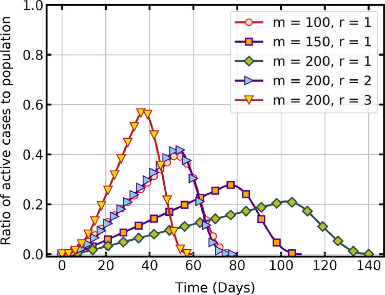
Fig. 3 shows that, when $r$ is held constant at 1, for a lattice dimension of $m=100$ the active infections reach a peak of 39.4% on day 52, and the entire population is infected and recovered in 77 days. For lattice dimensions $m=200$, the peak is 21.1% on day 102, and it takes 140 days for infection and recovery of the entire population. The maximum transmission $R_t$ and recovery time $t_R$ determine infection and recovery rates in the model. Both parameters are held constant in these simulations. The number of active cases thus linearly increases as the disease spreads in the fixed population and decreases rapidly after the peak value when the recovery rate dominates the infection rate. Evidently, as the size of the population increases, it takes more days to infect all. For the case $m=200$, when the range $r=3$, the rate of propagation is steep, with a peak of 57.2% on day 37 and recovery on day 59. Hence, the rate of virus transmission is slow in a large population compared to that in a small population when the range $r$ is held constant. Whereas, the per-day infection increases with an increase in the range $r$, resulting in a rapid propagation of virus in a population of constant size.

Fig. 3.

Temporal evolution of active infections with cellular automata parameters ($L_p=1,I_p=4,t_R=14$).

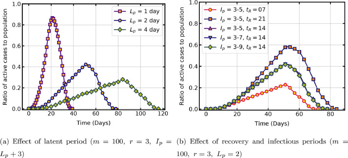
The effect of significant infection characteristics such as latent period, infectious period and recovery period on the progress of the pandemic is now studied. The latent period is the time taken for the virus to develop the ability to transmit after infecting a host. Fig. 4 a shows that, latent period has a sensitive influence on the model output when other parameters are held constant. When the latent period is one day, the virus transmission is rapid in the population and when it is four days, the virus transmission occurs at a slower rate. In these simulations, lattice size is $m=100$ and range $r=3$. The rapid rise and decline of the $L_p=1$ trajectory is also because of the change in range $r=3$, as a comparison with same latent period curve in Fig. 3 ($m=100,r=1$) shows. For the COVID-19 pandemic, studies report a latent period of 2 to 6 days [48], and as mentioned in Section. 2.1, the model is flexible to include such range of values.

Fig. 4.

Temporal evolution of active infections with infection characteristics.

Another important period in the life-cycle of the virus is the infectious period during which the virus remains contagious and its transmission occurs through various spread mechanisms. If the infectious period is more, the host could transmit the virus to many people. The present CA configuration, however, has limitations in capturing this fact, as a host in an infectious state is restricted to transmit only to the $S$ state cells in its transmittable neighbourhood. As the infectious period is increased, the host cell may be in the infectious state, but this is not reflected in the rate of pandemic propagation, as no additional susceptible cells are available to infect in the neighbourhood. The identical time trajectory with different infectious periods and same average recovery time $t_R=14$ days, shown in Fig. 4b, is attributed to this constraint in the present model. Fig. 4b also shows the effect of average recovery time of the disease, $t_R$, on rate of propagation. Clearly, when $t_R=21$, the peak of active cases is high compared to that for $t_R=7$ or 14. In the model recovery period $t_R$ is user-defined, and hence it is easy to adapt the value reported by authorities.

4. Results and discussions

Control measures such as lockdowns, steps such as relaxing restrictions and allowing migration of people to revive the economy and resume daily life and mitigation strategies such as vaccination roll out are some of the vital phases observed in the course of the COVID-19 pandemic. The developed model is used to carry out a parametric study to simulate these phases and the results are discussed in this section.

4.1. Effect of lockdown on time trajectory of pandemic

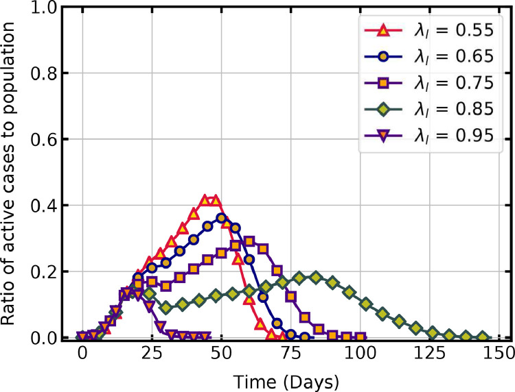
Lockdowns aim to prevent the movement and interaction of people and thus break the chain of the transmission cycle. As described in Section 2.3, the social isolation factor for the locality ${\lambda }_l$, is the parameter that indicates the intensity of lockdown in that region. In the simulations, the value of ${\lambda }_l$ is 0 at the start, and on the day of lockdown it is changed to a higher value by invoking a subroutine. The randomly generated social isolation factor for the infected person ${\lambda }_p$, is then compared with ${\lambda }_l$. Virus transmission can happen if ${\lambda }_p\ge {\lambda }_l$. The probability of ${\lambda }_p\ge {\lambda }_l$ reduces with an increase in ${\lambda }_l$ during the lockdown, thus reducing the rate of virus transmission. If there is no lockdown, then all infected individual could transmit the virus to their susceptible contacts. The reduction in the rate of infection with the increase in values of ${\lambda }_l$, imposed on day 15 onwards, is shown in Fig. 5 .

Fig. 5.

Temporal evolution of active infections with lockdown conditions.

A lower value of ${\lambda }_l$ shows a higher rate of infection propagation. As ${\lambda }_l$ is increased from 0.55 to 0.85, the rate of virus transmission decreases as indicated by the change in slope of active cases. For ${\lambda }_l=0.55$, the peak of active cases is 42.2 % on the 46th day, and all individuals are infected and recovered in 75 days. When ${\lambda }_l=0.85$, the rate of virus transmission is slow and the peak cases has a lower value of 18.4 % on the 83rd day but it takes 147 days for all active cases to recover. The different values of infection rate before and after imposing lockdown leads to the two local peaks observed on this curve. It can be seen that when ${\lambda }_l$ = 0.95, the number of active cases rapidly declines after imposing lockdown and reaches zero in 46 days. Only a few individuals are infected in this case which emphasizes the significance of strict lockdown on mitigating the pandemic. When ${\lambda }_l$ = 0.65 or 0.75, lockdown is not very effective and the entire population is infected eventually.

Previous studies show that a high percentage of reduced contacts through social isolation limits the spread of new cases [39], [47]. The timing of enforcing lockdown restrictions is also crucial, with earlier implementations leading to lesser infections [3], [5]. The present study also agrees with these results. In lockdown situations, if movement and interaction of people are there, then the infection will spread gradually with a smaller peak but for a longer duration. The healthcare system may not collapse but might exhaust the resources and people involved in it. Aggressive lockdown can curb the curve in a short span without infection spreading to a large section of the population. Different non-pharmaceutical interventions have varying effects on disease transmission [6], and the present model can provide initial estimates of such interventions by choosing appropriate values of social isolation factors.

4.2. Effect of migration on time trajectory of pandemic

Migration changes the size of the population and the dynamics of the pandemic. In a closely monitored and controlled region, the number of people migrating by various modes of transportation is accurately registered. The size of the cellular automata is incremented by a value $\delta$ in each time step to account for the migrating population. It is assumed that people are only migrating into the region and not moving out, so the size of the lattice only increases. In the migrating population, susceptible as well as exposed (infected) people will be present. Exposed states are assigned proportionally and distributed randomly in the lattice in each time step to account for this.

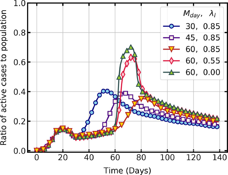
We studied two factors of importance in allowing migration in a region. First, the day on which migration can be started in a region with lockdown restrictions and second, the relaxations in lockdown that can be allowed during migration. Fig. 6 shows a comparison of active cases per day when migration is allowed on day 30, 45 and 60 with strict lockdown conditions of ${\lambda }_l=0.85$ and $\delta =5$. In all three cases, the second surge of active infections happens, which gradually declines with time. The increase in susceptible population and infection rate due to migration results in the second higher peak observed in these cases. For migration day 30, the peak of active cases is 40.7 % on day 53, and for migration day 60, the peak is 35.2 % on day 82.

Fig. 6.

Temporal evolution of active infections with different migration conditions ($M_{day}$ is migration start day).

The effect of relaxing the lockdown restrictions during migration is also shown in Fig. 6. The active cases per day under different lockdown conditions of ${\lambda }_l$ = 0.85 and 0.55 are compared with no lockdown condition of ${\lambda }_l$ = 0 for migration start day of 60. Relaxing the lockdown restrictions during migration rapidly increases the active cases close to that of ${\lambda }_l=0$. A sharp decline that follows is due to a high rate of recovery in comparison to new infections.

The results are in line with the observations of Sirakoulis et al. [32], that movement of people increases the overall infected population. A second surge is unavoidable during migration, but delaying the process can limit the peak of active cases. The spread of infections is also closely linked to the interactions between people as described in Section. 4.1. The surge in infections observed in delayed migration is due to this fact. Thus, the results infer that migration should be allowed only under strict lockdown conditions so that the peak of active cases is limited to a manageable level.

4.3. Effect of vaccination on time trajectory of pandemic

Universal immunisation is the scientific solution to control and mitigate a pandemic. As inoculation drive is a time-consuming process, it is vital to study the effect of various factors of vaccination program on infection reduction to aid in formulating a vaccination policy. In the present work, we look at how three such factors, $C_v$, $r_v$ and $d_v$ influence the dynamics of COVID-19. Here $C_v$ is the per day capacity of the healthcare system to administer vaccination, $r_v$ is the rate parameter of vaccination and $d_v$ is the day on which vaccination is started,

To simulate the vaccination program, the number of people to be vaccinated in each time step is estimated as a function of $C_v$ and $r_v$. An equal number of people in the susceptible state are then randomly selected and marked as vaccinated in the lattice [32]. A value of $v=16$, which is higher than the recovered state value, is assigned for vaccinated states to identify them as immune individuals. Since the health system capacity limits the maximum vaccinations per day, in the model a logistic function that converges to this capacity estimates the per-day registrations $R_v$. Time delay in reaching this maximum per day capacity depends on factors such as availability of vaccine and hesitancy of people, which is accounted by the rate parameter $r_v$ in the function.

$$R_v=\frac{C_v}{1+\frac{C_v-R_i}{R_i}{e}^{-r_{v}t}}$$ (3)

The logistic function is shown in Eq. (3), in which the per day vaccination capacity $C_v$ is provided as a percentage of total susceptible population, $t$ is the time step and $R_i$ represents the initial registration on $d_v=1$. In the following simulations, $C_v$ = 0.01, $r_v=0.6$, $d_v=1$ and $R_i$ = 1 unless otherwise specified.

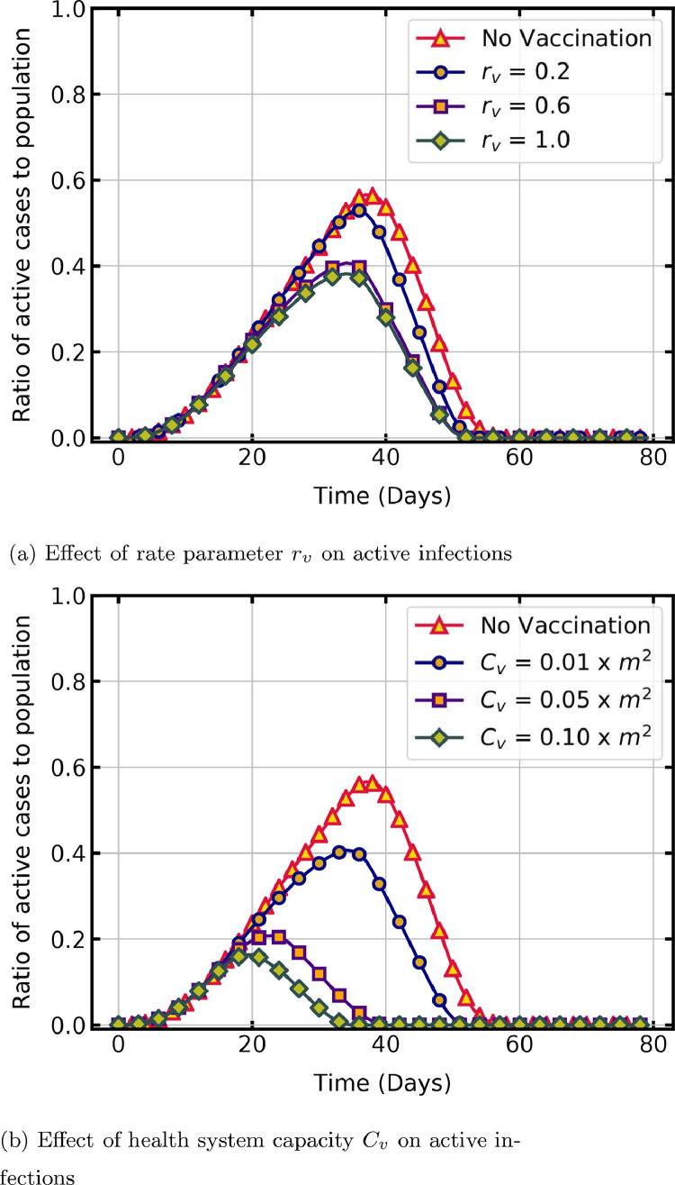
Fig. 7 a shows the effect of rate parameter $r_v$ on peak and duration of the pandemic. A notable reduction in per day active infections is observed with an increase in $r_v$. The peak percentage of active infections with $r_v$ = 0.2 is 53 % on day 36 and it reduces to 38 % on day 34 with an increase in $r_v$ = 1. An increase in $r_v$ from 0.2 to 0.6 significantly reduces the peak cases, whereas further change to 1 does not, because in the logistic function $r_v$ has an exponential influence on the growth of per day registration. The duration of the pandemic is comparable in all the cases as it mainly depends on the recovery time.

Fig. 7.

Temporal evolution of active infections with parameters estimating number of vaccinations per day.

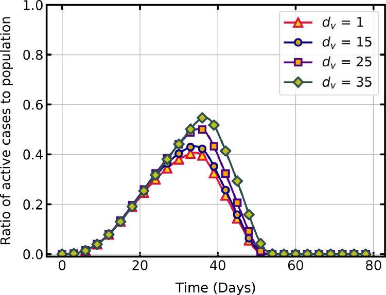
Fig. 7 b shows a comparison of the time trajectory of active cases without vaccination and with different vaccination capacities. As $C_v$ increases, the peak of active cases reduces due to the quick rise in the immune population. If $C_v$ is at least 10% of the susceptible population, then a substantial decline in active infections and duration of the pandemic is observed. Starting the vaccination campaign at the earliest possible day reduces the peak of active cases (Fig. 8 ) and subsequently the pressure on healthcare system. The peak cases is 56.6 % on day 37 without vaccination, whereas it is 50 % on day 35 for $d_v$ = 25 and 40.8 % on day 34, for $d_v$ = 0.

Fig. 8.

Effect of vaccination start day $d_v$ on active infections.

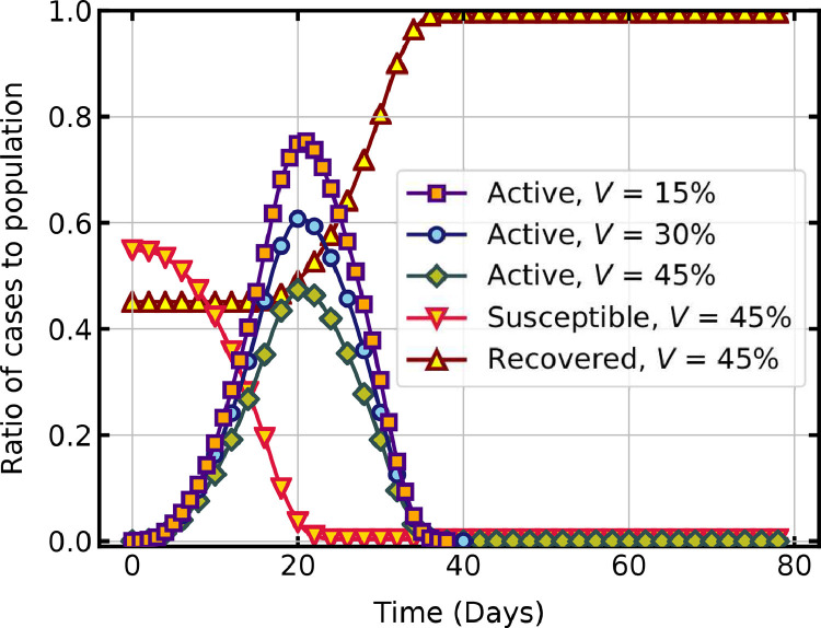
The present model is also used to investigate the peak and duration of a second wave of infection in a partially vaccinated population. An immune state $V$ is assigned for vaccinated people in the initial configuration of the lattice. As shown in Fig. 9 , when the percentage of the immune population is increased from $V=15\%$ to 30% and 45%, the peak of the active infections is seen to reduce significantly. The decline in susceptible population and increase in recovered population with an initial immune population of $V=45\%$ is also shown in this figure.

Fig. 9.

COVID-19 spread in a partially vaccinated population.

The results show that an increase in the percentage of the vaccinated population slows down the spread of new infections. An accelerated vaccine rollout and adherence to non-pharmaceutical interventions until adequate vaccination coverage are critical in controlling the COVID-19 pandemic [8]. Initially, people received the COVID-19 vaccination campaign with hesitancy due to various concerns [9], and now there is a shortage of supply. The model can forecast the overall impact of the vaccination program and prioritise population subgroups for effective inoculation.

4.4. Model performance and validation

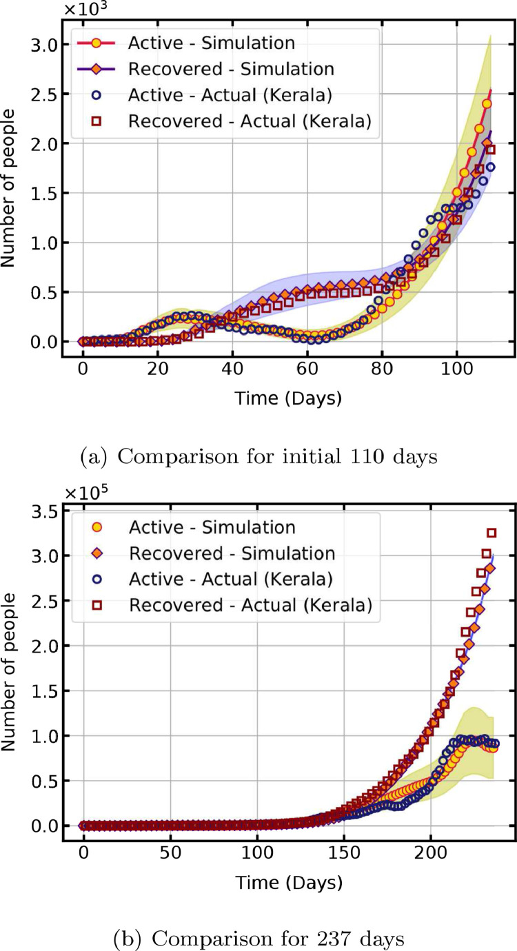
To assess the performance of the computational model and to validate the results, a comparison of the simulated and actual pandemic propagation data for the state of Kerala, India, is done. The first case of the COVID-19 pandemic in India is reported in Kerala on 30 January 2020. The data for 237 days from 9 March 2020, when the first wave of infections started, to 31 October 2020 is used for comparison [49]. A statewide lockdown is declared from 23 March 2020, and after lifting of restrictions in phases, notable migration to the state started on 7 May 2020, which are equal to 15th and 60th day respectively from 9 March 2020.

Table 3 lists the model parameters used in the validation. All other parameters are same as given in Table 2. The lockdown and migration conditions are simulated by changing the value of parameters on day 15 and 60. From day 60, the size of the lattice is proportionally increased ($m=m+\delta$) per time step to account for the change in susceptible population. The additional exposed cases introduced due to migration is taken as 4% of the population. Fig. 10 a shows a comparison for the first 110 days, with lockdown starting on day 15 and migration starting on day 60. Time taken for 1000 iterations for statistical analysis is 112 min. The shaded region indicates the confidence interval with a cumulative probability of 95%. The results establish the ability of the present model to reproduce the trajectory of the pandemic with appropriate values of model parameters.

Table 3.

Model parameters used in validation.

Common parameters (Notation)	Value
Initial parameters
Lattice dimension $\left(m\right)$	25
Infection parameters
Latent period$\left(L_p\right)$	2 days
Infectious period $\left(I_p\right)$	3 - 6 days
Recovery time $\left(t_R\right)$	14 days
Social isolation factor $\left({\lambda }_l\right)$	0.1
Simulation for 110 days
Lockdown (day 15)	${\lambda }_l=0.75$
Migration (day 60)	${\lambda }_l=0.60$, $\delta =5$
Simulation for 237 days
Lockdown (day 15)	${\lambda }_l=0.75$
Migration (day 60)	${\lambda }_l=0.60$, $\delta =1$
Relaxing restrictions (day 110)	${\lambda }_l=0.50$, $\delta =4$
Flattening of curve (day 220)	${\lambda }_l=0.65$, $\delta =1$

Fig. 10.

Validation of simulated results with actual data from Kerala, India.

The forecast for longer durations with constant model parameters resulted in the divergence of the trajectory with an increase in population. To improve the results, the parameters are changed in selected intervals and an estimate of incoming infections based on actual data is given as input. The model parameters are changed on day 60, 110 and 220 as shown in Table 3. The percentage of infected individuals in the incoming population is estimated from the actual data as the ratio of the seven-day rolling average of infections to the seven-day rolling average of individuals in quarantine. Fig. 10b shows a close comparison of actual and simulated data for a longer duration of 237 days. For this case, it takes 186 min to complete 50 iterations for the statistical analysis. Hence, the model with appropriately estimated parameters from actual data forecasts the dynamics with many infections in a longer duration.

Realistic forecasting of the time trajectory of the pandemic is obtained with few parameters when the population size is small. As the size of the population increases, the results deviate from actual data and simulating the exact trajectory requires changing the values of model parameters in smaller intervals of time. Hence, the presented model with simple transition rules and neighbourhood schemes is ideal for simulating COVID-19 outbreak in a population subgroup with fewer computational resources and time.

5. Conclusion

The unprecedented crisis of the COVID-19 pandemic has affected the lives of millions of people across the world. Decentralised cluster containment, which concentrates on small regions or population subgroups, facilitates early detection and isolation of infected cases and efficient use of resources in the long run. This study proposes a computational model based on probabilistic cellular automata for forecasting the peak and duration of the COVID-19 propagation in a cluster under various conditions. The cellular automata configuration consists of a two-dimensional regular lattice, representing a population subgroup, with each of its cell representing a person at a particular stage of pandemic. A transmittable and transmission neighbourhoods are defined around a single host to identify the most probable susceptible individuals. The transition rule states that virus transmission occurs when susceptible individuals are present in the transmittable neighbourhood of the infected individual and violates the conditions of social isolation. The size of the lattice is increased proportionally to accommodate incoming susceptible and infectious populations during migration.

The sensitivity of model parameters such as the size of the susceptible population, range of the transmittable neighbourhood and various disease characteristics on the time trajectory of the pandemic is simulated first. A statistical analysis of the output shows a variation of results within 1% of the mean data. The impact of lockdown, migration and vaccination on the dynamics of the pandemic is then studied. Results indicate that stringent lockdown, controlled migration under strict social isolation conditions and a higher vaccination capacity is essential for a smaller peak and duration of the pandemic. The model performance is assessed and validated by simulating and comparing the results with actual COVID-19 data from the state of Kerala in India.

Simulations using the present model, with minimum parameters and computational requirements, can provide valuable insights into evolving disease dynamics in a cluster for effective decision making and quick response. Improvements by including fluctuations in migrating population, using scientifically estimated social isolation factors and testing different vaccination scenarios with real data will enable the model to forecast the long-term behaviour of the pandemic.

Declaration of Competing Interest

The authors declare that they have no known competing financial interests or personal relationships that could have appeared to influence the work reported in this paper.

Appendix A. Supplementary materials

Supplementary Data S1

Supplementary Raw Research Data. This is open data under the CC BY license http://creativecommons.org/licenses/by/4.0/

References

- 1.Cucinotta D., Vanelli M. Who declares COVID-19 a pandemic. Acta Biomed. 2020;91(1):157–160. doi: 10.23750/abm.v91i1.9397. [DOI] [PMC free article] [PubMed] [Google Scholar]
- 2.Pai C., Bhaskar A., Rawoot V. Investigating the dynamics of COVID-19 pandemic in India under lockdown. Chaos Solitons Fractals. 2020;138:109988. doi: 10.1016/j.chaos.2020.109988. [DOI] [PMC free article] [PubMed] [Google Scholar]
- 3.Giordano G., Blanchini F., Bruno R., Colaneri P., Di Filippo A., Di Matteo A., Colaneri M. Modelling the COVID-19 epidemic and implementation of population-wide interventions in Italy. Nat. Med. 2020;26(6):855–860. doi: 10.1038/s41591-020-0883-7. [DOI] [PMC free article] [PubMed] [Google Scholar]
- 4.Han E., Tan M.M.J., Turk E., Sridhar D., Leung G.M., Shibuya K., Asgari N., Oh J., Garcȡa-Basteiro A.L., Hanefeld J., Cook A.R., Hsu L.Y., Teo Y.Y., Heymann D., Clark H., McKee M., Legido-Quigley H. Lessons learnt from easing COVID-19 restrictions: an analysis of countries and regions in Asia pacific and Europe. Lancet. 2020;396(10261):1525–1534. doi: 10.1016/S0140-6736(20)32007-9. [DOI] [PMC free article] [PubMed] [Google Scholar]
- 5.Post R.A.J., Regis M., Zhan Z., van den Heuvel E.R. How did governmental interventions affect the spread of COVID-19 in European countries? BMC Public Health. 2021;21(1):411. doi: 10.1186/s12889-021-10257-2. [DOI] [PMC free article] [PubMed] [Google Scholar]
- 6.Brauner J.M., Mindermann S., Sharma M., Johnston D., Salvatier J., Gavenčiak T., Stephenson A.B., Leech G., Altman G., Mikulik V., Norman A.J., Monrad J.T., Besiroglu T., Ge H., Hartwick M.A., Teh Y.W., Chindelevitch L., Gal Y., Kulveit J. Inferring the effectiveness of government interventions against COVID-19. Science. 2021;371(6531) doi: 10.1126/science.abd9338. [DOI] [PMC free article] [PubMed] [Google Scholar]
- 7.Ibn-Mohammed T., Mustapha K.B., Godsell J., Adamu Z., Babatunde K.A., Akintade D.D., Acquaye A., Fujii H., Ndiaye M.M., Yamoah F.A., Koh S.C.L. A critical analysis of the impacts of COVID-19 on the global economy and ecosystems and opportunities for circular economy strategies. Resour. Conserv. Recycl. 2021;164:105169. doi: 10.1016/j.resconrec.2020.105169. [DOI] [PMC free article] [PubMed] [Google Scholar]
- 8.Vilches T.N., Zhang K., Van Exan R., Langley J.M., Moghadas S.M. Projecting the impact of a two-dose COVID-19 vaccination Campaign in Ontario, Canada. Vaccine. 2021;39(17):2360–2365. doi: 10.1016/j.vaccine.2021.03.058. [DOI] [PMC free article] [PubMed] [Google Scholar]
- 9.Lazarus J.V., Ratzan S.C., Palayew A., Gostin L.O., Larson H.J., Rabin K., Kimball S., El-Mohandes A. A global survey of potential acceptance of a COVID-19 vaccine. Nat. Med. 2021;27(2):225–228. doi: 10.1038/s41591-020-1124-9. [DOI] [PMC free article] [PubMed] [Google Scholar]
- 10.Ceylan Z. Estimation of COVID-19 prevalence in Italy, Spain, and France. Sci. Total Environ. 2020;729:138817. doi: 10.1016/j.scitotenv.2020.138817. [DOI] [PMC free article] [PubMed] [Google Scholar]
- 11.Sahoo B.K., Sapra B.K. A data driven epidemic model to analyse the lockdown effect and predict the course of COVID-19 progress in India. Chaos Solitons Fractals. 2020;139:110034. doi: 10.1016/j.chaos.2020.110034. [DOI] [PMC free article] [PubMed] [Google Scholar]
- 12.Chatterjee K., Chatterjee K., Kumar A., Shankar S. Healthcare impact of COVID-19 epidemic in India: a stochastic mathematical model. Med. J. Armed Forces India. 2020;76(2):147–155. doi: 10.1016/j.mjafi.2020.03.022. [DOI] [PMC free article] [PubMed] [Google Scholar]
- 13.Mac S., Mishra S., Ximenes R., Barrett K., Khan Y.A., Naimark D., Sander B. Modeling the COVID-19 pandemic: a comprehensive guide of infectious disease and decision-analytic models. J. Clin. Epidemiol. 2020 doi: 10.1016/j.jclinepi.2020.12.002. [DOI] [PMC free article] [PubMed] [Google Scholar]
- 14.Xiang Y., Jia Y., Chen L., Guo L., Shu B., Long E. COVID-19 epidemic prediction and the impact of public health interventions: a review of COVID-19 epidemic models. Infect. Dis. Model. 2021;6:324–342. doi: 10.1016/j.idm.2021.01.001. [DOI] [PMC free article] [PubMed] [Google Scholar]
- 15.White S.H., del Rey A.M., Sánchez G.R. Modeling epidemics using cellular automata. Appl. Math. Comput. 2007;186(1):193–202. doi: 10.1016/j.amc.2006.06.126. [DOI] [PMC free article] [PubMed] [Google Scholar]
- 16.Kretzschmar M., Wallinga J. Modern Infectious Disease Epidemiology: Concepts, Methods, Mathematical Models, and Public Health. 2009. Mathematical models in infectious disease epidemiology; pp. 209–221. [Google Scholar]
- 17.Brauer F. Mathematical epidemiology: past, present, and future. Infect. Dis. Model. 2017;2(2):113–127. doi: 10.1016/j.idm.2017.02.001. [DOI] [PMC free article] [PubMed] [Google Scholar]
- 18.Rahimi I., Chen F., Gandomi A.H. A review on COVID-19 forecasting models. Neural Comput. Appl. 2021 doi: 10.1007/s00521-020-05626-8. [DOI] [PMC free article] [PubMed] [Google Scholar]
- 19.Macías-Díaz J.E., Raza A., Ahmed N., Rafiq M. Analysis of a nonstandard computer method to simulate a nonlinear stochastic epidemiological model of coronavirus-like diseases. Comput. Methods Programs Biomed. 2021;204:106054. doi: 10.1016/j.cmpb.2021.106054. [DOI] [PMC free article] [PubMed] [Google Scholar]
- 20.Arino J., Brauer F., van den Driessche P., Watmough J., Wu J. Simple models for containment of a pandemic. J. R. Soc. Interface. 2006;3(8):453–457. doi: 10.1098/rsif.2006.0112. [DOI] [PMC free article] [PubMed] [Google Scholar]
- 21.Huppert A., Katriel G. Mathematical modelling and prediction in infectious disease epidemiology. Clin. Microbiol. Infect. 2013;19(11):999–1005. doi: 10.1111/1469-0691.12308. [DOI] [PubMed] [Google Scholar]
- 22.Athithan S., Shukla V.P., Biradar S.R. Dynamic cellular automata based epidemic spread model for population in patches with movement. J. Comput. Environ. Sci. 2014;2014:518053. doi: 10.1155/2014/518053. [DOI] [Google Scholar]
- 23.Holko A., Medrek M., Pastuszak Z., Phusavat K. Epidemiological modeling with a population density map-based cellular automata simulation system. Expert Syst. Appl. 2016;48:1–8. [Google Scholar]
- 24.Sharma N., Gupta A.K. Impact of time delay on the dynamics of SEIR epidemic model using cellular automata. Physica A. 2017;471:114–125. [Google Scholar]
- 25.Liang K. Mathematical model of infection kinetics and its analysis for COVID-19, SARS and MERS. Infect. Genet. Evol. 2020;82:104306. doi: 10.1016/j.meegid.2020.104306. [DOI] [PMC free article] [PubMed] [Google Scholar]
- 26.Ivorra B., Ferrndez M.R., Vela-PȨrez M., Ramos A.M. Mathematical modeling of the spread of the coronavirus disease 2019 (COVID-19) taking into account the undetected infections. the case of China. Commun. Nonlinear Sci. Numer.Simul. 2020;88:105303. doi: 10.1016/j.cnsns.2020.105303. [DOI] [PMC free article] [PubMed] [Google Scholar]
- 27.Kucharski A.J., Russell T.W., Diamond C., Liu Y., Edmunds J., Funk S., Eggo R.M., Sun F., Jit M., Munday J.D., Davies N., Gimma A., van Zandvoort K., Gibbs H., Hellewell J., Jarvis C.I., Clifford S., Quilty B.J., Bosse N.I., Abbott S., Klepac P., Flasche S. Early dynamics of transmission and control of COVID-19: a mathematical modelling study. Lancet Infect. Dis. 2020;20(5):553–558. doi: 10.1016/S1473-3099(20)30144-4. [DOI] [PMC free article] [PubMed] [Google Scholar]
- 28.Gumel A.B., Iboi E.A., Ngonghala C.N., Elbasha E.H. A primer on using mathematics to understand COVID-19 dynamics: modeling, analysis and simulations. Infect. Dis. Model. 2021;6:148–168. doi: 10.1016/j.idm.2020.11.005. [DOI] [PMC free article] [PubMed] [Google Scholar]
- 29.Shoaib M., Raja M.A.Z., Sabir M.T., Bukhari A.H., Alrabaiah H., Shah Z., Kumam P., Islam S. A stochastic numerical analysis based on hybrid NAR-RBFs networks nonlinear SITR model for novel COVID-19 dynamics. Comput. Methods Programs Biomed. 2021;202:105973. doi: 10.1016/j.cmpb.2021.105973. [DOI] [PMC free article] [PubMed] [Google Scholar]
- 30.Padmanabhan R., Abed H.S., Meskin N., Khattab T., Shraim M., Al-Hitmi M.A. A review of mathematical model-based scenario analysis and interventions for COVID-19. Comput. Methods Programs Biomed. 2021;209:106301. doi: 10.1016/j.cmpb.2021.106301. [DOI] [PMC free article] [PubMed] [Google Scholar]
- 31.Ahmed E., Agiza H.N. On modeling epidemics including latency, incubation and variable susceptibility. Physica A. 1998;253(1):347–352. [Google Scholar]
- 32.Sirakoulis G.C., Karafyllidis I., Thanailakis A. A cellular automaton model for the effects of population movement and vaccination on epidemic propagation. Ecol. Model. 2000;133(3):209–223. [Google Scholar]
- 33.Ahmed E., Elgazzar A.S. On some applications of cellular automata. Physica A. 2001;296(3):529–538. [Google Scholar]
- 34.Monteiro L.H.A., Fanti V.C., Tessaro A.S. On the spread of SARS-CoV-2 under quarantine: a study based on probabilistic cellular automaton. Ecol. Complexity. 2020;44:100879. [Google Scholar]
- 35.Salcido A. A lattice gas model for infection spreading: application to the COVID-19 pandemic in the mexico city metropolitan area. Results Phys. 2021;20:103758. doi: 10.1016/j.rinp.2020.103758. [DOI] [PMC free article] [PubMed] [Google Scholar]
- 36.Ghaemi M. An investigation of the effects of lifting quarantine conditions after the peak of COVID-19 pandemic using the cellular automata approach. Res. Square. 2021 [Google Scholar]
- 37.Ghosh S., Bhattacharya S. A data-driven understanding of COVID-19 dynamics using sequential genetic algorithm based probabilistic cellular automata. Appl. Soft Comput. 2020;96:106692. doi: 10.1016/j.asoc.2020.106692. [DOI] [PMC free article] [PubMed] [Google Scholar]
- 38.Ghosh S., Bhattacharya S. Computational model on COVID-19 pandemic using probabilistic cellular automata. SN Comput. Sci. 2021;2(3):230. doi: 10.1007/s42979-021-00619-3. [DOI] [PMC free article] [PubMed] [Google Scholar]
- 39.Schimit P.H.T. A model based on cellular automata to estimate the social isolation impact on COVID-19 spreading in Brazil. Comput. Methods Programs Biomed. 2021;200:105832. doi: 10.1016/j.cmpb.2020.105832. [DOI] [PMC free article] [PubMed] [Google Scholar]
- 40.Zhou Y., Wang L., Zhang L., Shi L., Yang K., He J., Zhao B., Overton W., Purkayastha S., Song P. A spatiotemporal epidemiological prediction model to inform county-level COVID-19 risk in the United States. Harvard Data Sci. Rev. 2020 doi: 10.1162/99608f92.79e1f45e. [DOI] [Google Scholar]; https://hdsr.mitpress.mit.edu/pub/qqg19a0r
- 41.J. Dai, C. Zhai, J. Ai, J. Ma, J. Wang, W. Sun, Modeling the spread of epidemics based on cellular automata, 2021,
- 42.Meghwal B., Behera S., Dhariwal A., Saxena D., Singh R., Kumar S. Insights from COVID-19 cluster containment in Bhilwara district, Rajasthan. Indian J. Public Health. 2020;64(6):177–182. doi: 10.4103/ijph.IJPH_489_20. [DOI] [PubMed] [Google Scholar]
- 43.Cartocci A., Cevenini G., Barbini P. A compartment modeling approach to reconstruct and analyze gender and age-grouped COVID-19 Italian data for decision-making strategies. J. Biomed. Inf. 2021;118:103793. doi: 10.1016/j.jbi.2021.103793. [DOI] [PMC free article] [PubMed] [Google Scholar]
- 44.Chopard B., Dupuis A., Masselot A., Luthi P. Cellular automata and lattice Boltzmann techniques: an approach to model and simulate complex systems. Adv. Complex Syst. 2002;05(02n03):103–246. doi: 10.1142/s0219525902000602. [DOI] [Google Scholar]
- 45.El Yacoubi S., El Jai A. Cellular automata modelling and spreadability. Math. Comput. Model. 2002;36(9):1059–1074. [Google Scholar]
- 46.WHO . Technical Report. World Health Organisation; Scientific brief: 2020. Transmission of SARS-CoV-2: Implications for Infection Prevention Precautions. [Google Scholar]
- 47.Wang Y., Li B., Gouripeddi R., Facelli J.C. Human activity pattern implications for modeling SARS-CoV-2 transmission. Comput. Methods Programs Biomed. 2021;199:105896. doi: 10.1016/j.cmpb.2020.105896. [DOI] [PMC free article] [PubMed] [Google Scholar]
- 48.Sanche S., Lin Y.T., Xu C., Romero-Severson E., Hengartner N., Ke R. High contagiousness and rapid spread of severe acute respiratory syndrome coronavirus 2. Emerg. Infect. Dis. 2020;26(7):1470–1477. doi: 10.3201/eid2607.200282. [DOI] [PMC free article] [PubMed] [Google Scholar]
- 49.Health & Family Welfare Department G.o.K. Daily Bulletins; 2020. COVID-19 Outbreak Control and Prevention State Cell. [Google Scholar]
Associated Data
This section collects any data citations, data availability statements, or supplementary materials included in this article.
Supplementary Materials