An epidemic model through information-induced vaccination and treatment under fuzzy impreciseness

Abstract

In this work, we propose a nonlinear susceptible (S), vaccinated (V), infective (I), recovered (R), information level (U) (SVIRUS) model for the dynamical behavior of the contagious disease in human beings. We mainly consider the spread of information during the course of epidemic in the population. Different rate equations describe the dynamics of the information. We have developed the proposed model in crisp and fuzzy environments. In the fuzzy model, to describe the uncertainty prevailed in the dynamics, all the parameters are taken as triangular fuzzy numbers. Using graded mean integration value (GMIV) method, the fuzzy model is transformed into defuzzified model to represent the solutions avoiding the difficulties. The positivity and the boundedness of the crisp model are discussed elaborately and also the equilibrium analysis is accomplished. The stability analysis for both the infection free and the infected equilibrium are established for the crisp model. Application of optimal control of the crisp system is explored. Using Pontryagin’s Maximum Principle, the optimal control is explained. The effect of vaccination is analyzed which leads the model to be complex in nature. The effect of saturation constant for information is described for the crisp model and also the effects of weight constants on control policy are discussed. Finally, it is concluded that the treatment is more fruitful and information related vaccination is more effective during the course of epidemic.

Introduction

A lot of attention has been drawn by infectious diseases in our society in recent time. Sometimes these infectious diseases are most dangerous and become epidemics. Recently, the infectious diseases, such as influenza, chicken pox, SARS, etc. have been spread dangerously and created panic throughout the world. The spread of these diseases affects the development plans for the infected countries (Russell 2004; Gupta et al. 2005) and also to the world economy. The productivity losses, health-related expenditures, employments, travels and tourisms, etc. are being totally hampered due to the occurrences of several epidemics. Therefore, the controlling of the spread of infectious diseases (Raeei 2020; Akdim et al. 2021; Roy et al. 2021; Gupta et al. 2020) as well as the minimization of the whole cost incurred during the epidemic times, are the important tasks for the policy makers and the administrative authorities of the government.

In recent years, the scientists, the doctors, the researchers, the medical facility providers, pharmaceutical units and other related units including the government are facing challenges due to complicated characteristics of the diseases. So, the study of the mathematical modeling of the infectious diseases is one of the most effective tools to predict and analyze the behaviour of the infectious diseases (Brauer and Chavez 2012). Many researchers (Joshi et al. 2006; Zaman et al. 2008) used the controlling interventions like vaccination, treatment, quarantine, isolation, contact tracing, walk-in program, etc. to stop the spreading and to minimize the effects of the infectious diseases in the society. Various control interventions for bad impacts of the disease dynamics were studied by many researchers. They mainly used optimal control theory (Gaff and Schaefer 2009; Fleming and Rishel et al. 1975) in their investigations. Behncke (2000) investigated SIR epidemic model and in his work the effect of vaccination, screening, health-related campaigns were the main substances. They also suggested the control intervention for suppressing the disease level. Both the effects of information induced change in the contact pattern and vaccination system (Buonomo et al. 2012, 2013) were explained by Alberto d’Onofrio et al. (2007). Buonomo et al. (2013) considered an SEIR model with the effect of information related vaccination for new born. Many authors used awareness and effect of information as control strategy for HIV in their studies (Kassa and Ouhinou 2015). Kumar et al. (2016) discussed the mathematical model with information and explained the optimal control problem. Numerically, they investigated the results of saturated treatment on the optimal policies. Kumar et al. (2019) designed a SVIRM epidemic model. They discussed both the effect of vaccine working efficiency on optimal control and analyzed the cost efficient of the optimal controls of the contagious disease.

Zadeh (1965) first introduced fuzzy set theory to study the uncertainty in mathematics. Das and Pal (2018) proposed the imprecise epidemic system with optimal treatment and vaccination to control the epidemic. Researchers paid attention to develop the epidemic models in uncertain environments (Pontryagin et al. 1962; Panja et al. 2017; Mahata et al. 2018; Nandi et al. 2018; Das et al. 2020a). Das et al. (2020b) explained disease control eco-epidemic model with prey refuge under fuzzy uncertainty.

In this work, we have deigned an infectious disease model which has been developed by taking the control interventions as information induced vaccination and treatment. To cope up with the uncertainties prevailed in the control parameters; we consider the impreciseness in terms of fuzzy numbers. This imprecise model is more realistic to represent the real life unpredictable situations. Thus, in this work, we develop the imprecise model along with the crisp model. We analyze the crisp model for the positivity, boundedness, equilibrium analysis, stability and optimal control. The numerical experiments for both models are performed and the solutions, sensitivities of the parameters, effects of optimal control are presented graphically.

The entire paper is divided into several sections and sub-sections. Some useful preliminaries are described in “Some preliminaries” . “Model calibration” represents the model calibration. In “Positivity and boundedness of the crisp model”, the positivity and boundedness of the crisp model are discussed. “Equilibrium analysis” describes the equilibrium analysis of the crisp model. “Global stability analysis” presents the stability of the both equilibrium infection free and infected of the crisp model. The theory of optimal control is explained in “Application of optimal control”. The solution procedure of the model is described in the “Solution procedure”. In “Numerical results”, the numerical results of both the crisp model and the fuzzy model are performed. Finally, the concluding remarks are given in “Conclusions”.

Findings of this work

In our model, we presented the epidemic model in which the control strategies are information of vaccination and treatment. Further, to develop this model we introduce the optimal control. We design the model in precise and imprecise environments. In the imprecise model, the control parameters are assumed to behave as fuzzy parameters. The triangular fuzzy numbers are used to represent the uncertainties of the control parameters. It has been established from the analysis and numerical experiments that the result of the involvement of the information related to vaccination and treatment is more useful to mitigate the spread of the epidemic. The optimal control policy is effective to minimize the effect of the epidemic. It is explained that the use of both the information related to vaccination and treatment decrease the load of the disease. The model suggest through optimal control that the use of interventions like information of vaccination of unaffected persons and treatment of infected persons has important rule to decease the spread of epidemic and to reduce the overall effect of it.

Some preliminaries

In this section, we use some basic definitions.

Fuzzy number

The fuzzy set $\tilde{F}$ is called normal and convex, if the following conditions must be satisfied

• (i)${\mu }_{\tilde{F}}\left(t_0\right)=1$ for some $t_0$,
• (ii)${\mu }_{\tilde{F}}\left(\lambda ,t_1+\left(1-\lambda \right)t_2\right)\le \lambda {\mu }_{\tilde{F}}\left(t_1\right)+\left(1-\lambda \right){\mu }_{\tilde{F}}\left(t_2\right)$.

where, ${\mu }_{\tilde{F}}\left(t\right)$ is the membership function of the fuzzy number $\tilde{F}.$

GMIV formula of Fuzzy Number

In this work, we use the GMIV (graded mean integration value) technique of defuzzification (Chen and Hsieh 1999) which is given below.

If the parameter $m\in \left[0,1\right]$ represents the degree of optimism, then the GMIV of the fuzzy number $\tilde{F}$ is,

$$\begin{array}{c}{K}_f\left(\tilde{F}\right)=\frac{{\int }_0^1{t}_f\left\{\left(1-m\right)L_1^{-1}\left(t_f\right)+m{L}_2^{-1}\left(t_f\right)\right\}dt}{{\int }_0^1{t}_{f}d{t}_f}\\ =2\underset{0}{\overset{1}{\int }}{t}_f\left\{\left(1-m\right)L_1^{-1}\left(t_f\right)+m{L}_2^{-1}\left(t_f\right)\right\}d{t}_f\\ \end{array}$$

where, the left shape function and right shape function of $\tilde{F}$ are represented by $L_1(t_f)$ and $L_2(t_f)$ respectively.

GMIV of triangular fuzzy number (TFN)

Let us consider the TFN $\tilde{F}$= ($F_1,F_2,F_3$), whose membership function is

$${\mu }_{\tilde{F}}\left(t_f\right)=\left\{\begin{array}{cc}\frac{x-F_1}{F_2-F_1}\hfill & \text{if}{F}_1\le x\le F_2\hfill \\ 1\hfill & \text{if}x=F_2\hfill \\ \frac{F_3-x}{F_3-F_2}\hfill & \text{if}{F}_2\le x\le F_3\hfill \\ 0\hfill & \text{otherwise}\hfill \end{array}\right)$$

Then $L_1\left(t_f\right)=\frac{t_f-F_1}{F_2-F_1}$ and $L_2\left(t_f\right)=\frac{F_3-t_f}{F_3-F_2}.$

Therefore, $L_1^{-1}\left(t_f\right)=F_1+\left(F_2-F_1\right)t_f$ and $L_2^{-1}\left(t_f\right)=F_3-\left(F_3-F_2\right)t_f$.

So, GMIV of $\begin{array}{c}\tilde{F}=2\underset{0}{\overset{1}{\int }}{t}_f\left\{\left(1-m\right)L_1^{-1}\left(t_f\right)+m{L}_2^{-1}\left(t_f\right)\right\}d{t}_f\\ =2\underset{0}{\overset{1}{\int }}{t}_f\{\left(1-m\right)[F_1+\left(F_2-F_1\right)t_f\left]+m\right[F_3-\left(F_3-F_2\right)t_f]\}d{t}_f\\ =2\left[\left(1-m\right)\left\{\frac{F_2}{2}+\frac{\left(F_2-F_1\right)}{3}\right\}+m\left\{\frac{F_3}{2}-\frac{\left(F_3-F_2\right)}{3}\right\}\right]\\ =\frac{1}{3}\left[\left(1-m\right)F_1+2F_2+m{F}_3\right]\\ \end{array}$.

If we denote the GMIV of $\tilde{F}$ by $K_f\left(\tilde{F}\right)$, then

$K_f\left(\tilde{F}\right)=\frac{1}{3}\left[\left(1-m\right)F_1+2F_2+m{F}_3\right]$.

Model calibration

In this section, we develop the epidemic model in which the treatment and the information related to the vaccination are considered as the intervention control. We first develop the crisp model and then the imprecise fuzzy model.

Case 1: crisp model

Let us formulate a compartmental $\mathit{SVIRUS}$ epidemic model which describes the dynamics of the contagious diseases through the treatment and information related to the vaccination. We divide the total population ($N$) into sub populations as susceptible (S), vaccinated ($V$), infective ($I$), recovered ($R$) which are functions of any time $t$. The variable $U$ indicates information density available within the population for disease outbreak at time $t$. We take vaccination rate considering for the function of $U$ i.e., $q_0+\frac{v_{1}U}{1+{\theta }_{1}U}$, where $q_0$ is the baseline vaccination parameter, $v_1$ indicates the information related to the rate of vaccination in the susceptible individuals and ${\theta }_1$ is a constant relation with the saturation in information related to vaccination. We assume that vaccination does not fully work for protection. Therefore, the vaccinated individuals may be infectious again. Under these considerations, the nonlinear $\mathit{SVIRUS}$ model is represented by the following system of differential equations:

$$\begin{array}{c}\frac{\mathit{dS}}{\mathit{dt}}=\mathrm{\Pi }-\lambda SI-dS-\left(q_0+\frac{v_{1}U}{1+{\theta }_{1}U}\right)S+{\gamma }_{0}R\\ \frac{\mathit{dV}}{\mathit{dt}}=\left(q_0+\frac{v_{1}U}{1+{\theta }_{1}U}\right)S-\lambda \left(1-\psi \right)VI-\left(\beta +d\right)V\\ \frac{\mathit{dI}}{\mathit{dt}}=\lambda SI+\lambda \left(1-\psi \right)VI-\left(\gamma +d+\delta \right)I-\left(a+b{v}_2\right)I\\ \frac{\mathit{dR}}{\mathit{dt}}=\beta V+\gamma I-dR-{\gamma }_{0}R+\left(a+b{v}_2\right)I\\ \frac{\mathit{dU}}{\mathit{dt}}=gI-p_{0}U\\ \end{array}$$ 1

where, the initial value of the state variables are nonnegative at any instant $t$ and all the control parameters are considered as nonnegative. The parameter Π and $d$ indicate the inflow rate of susceptible individuals and the mortality rate for all populations respectively. We take the parameter $\lambda$ as disease transmission rate of susceptible individuals. $\psi (0\le \psi \le 1)$ is the efficiency rate of vaccination and $q_0$ is the vaccination base line parameter. Population get full protection when $\psi =1$ and get no immunity when $\psi =0$. The parameter $\beta$ represents vaccine related immunity rate. We take the parameter $\delta$ as the death rate due to the disease. At the time when both the baseline of vaccination is maintained and the information related to vaccination are applied, then the term $\left(q_0,+,\frac{v_{1}U}{1+{\theta }_{1}U}\right)S$ represents the growth of vaccinated population. We consider the parameter $v_1$ and ${\theta }_1$ as the information related to vaccination and saturation constant for information respectively. The parameter $v_2(0\le v_2\le 1)$ is related to treatment for infective population. Rate of effectiveness due to treatment is denoted by the parameter $b$. We take the parameter $a$ as natural recovery rate for all the population. So, the total recovery is $\left(a,+,b,v_2\right)$ of infective population. The parameter $g$ which denotes the growth rate of information is proportional to mass media, newspaper, social media, various educational campaigns, etc. The parameter ${\gamma }_0$ represents the loss of the protection rate of the recovered population and $p_0$ denotes the fading memory for information. The diagram and biological significance of the model (1) are presented in Fig. 1 and Table 1 respectively.

Fig. 1.

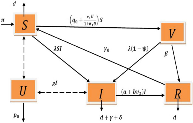
The diagram of the model (1)

Table 1.

Biological significance and parametric values for the crisp model (1)

Parameters	Biological significance	Values and units	Data source
$\mathrm{\Pi }$	Inflow rate	20 $\frac{1}{\mathrm{day}}$	Assumed
$\lambda$	Disease transmission rate of susceptible population	0.0002 $\frac{1}{\mathrm{day}}$	Kassa and Ouhinou (2015)
$d$	Natural mortality rate	0.00004 $\frac{1}{\mathrm{day}}$	Liu et al. (2008)
$q_0$	Vaccination rate	0.001 $\frac{1}{\mathrm{day}}$	Assumed
$v_1$	Control parameter	0.001	Lenhart and Workman (2007)
${\theta }_1$	Saturation constant for information	0.01	Zhang and Liu (2008)
${\gamma }_0$	Loss of the protection rate	0.001 $\frac{1}{\mathrm{day}}$	Assumed
$\psi$	Vaccine working efficiency rate	0.95 $\frac{1}{\mathrm{day}}$	Assumed
$\beta$	Vaccine related immunity rate	0.093 $\frac{1}{\mathrm{day}}$	Gumel and Ruan (2004)
$\gamma$	Recovery rate of infective	0.03 $\frac{1}{\mathrm{day}}$	Gumel and Ruan (2004)
$\delta$	Disease induced death rate	0.04 $\frac{1}{\mathrm{day}}$	Gumel and Ruan (2004)
$v_2$	Control parameter	0.001	Lenhart and Workman (2007)
$b$	Rate of effectiveness due to treatment	0.75 $\frac{1}{\mathrm{day}}$	Assumed
$g$	Growth rate for information	0.05 $\frac{1}{\mathrm{day}}$	Misra et al. (2011)
$a$	Natural recovery rate	0.001 $\frac{1}{\mathrm{day}}$	Assumed
$p_0$	Degradation rate for information	0.05 $\frac{1}{\mathrm{day}}$	Misra et al. (2011)

Case 2: fuzzy model

In this model, we take the parameters like that fuzzy numbers to consider the impreciseness. The system of differential equations given in (1) is transformed into the following system of fuzzy differential equations.

$$\begin{array}{c}\widetilde{\frac{\mathit{dS}}{\mathit{dt}}}=\tilde{\mathrm{\Pi }}-\tilde{\lambda }SI-\tilde{d}S-\left(\widetilde{q_0}+\frac{\widetilde{v_1}U}{1+\widetilde{{\theta }_1}U}\right)S+\widetilde{{\gamma }_0}R\\ \widetilde{\frac{\mathit{dV}}{\mathit{dt}}}=\left(\widetilde{q_0}+\frac{\widetilde{v_1}U}{1+\widetilde{{\theta }_1}U}\right)S-\tilde{\lambda }\left(1-\tilde{\psi }\right)VI-\left(\tilde{\beta }+\tilde{d}\right)V\\ \widetilde{\frac{\mathit{dI}}{\mathit{dt}}}=\tilde{\lambda }SI+\tilde{\lambda }\left(1-\tilde{\psi }\right)VI-\left(\tilde{\gamma }+\tilde{d}+\tilde{\delta }\right)I-\left(\tilde{a}+\tilde{b}\widetilde{v_2}\right)I\\ \widetilde{\frac{\mathit{dR}}{\mathit{dt}}}=\tilde{\beta }V+\tilde{\gamma }I-\tilde{d}R-\widetilde{{\gamma }_0}R+\left(\tilde{a}+\tilde{b}\widetilde{v_2}\right)I\\ \widetilde{\frac{\mathit{dU}}{\mathit{dt}}}=\tilde{g}I-\widetilde{p_0}U\\ \end{array}$$ 2

where, $\tilde{\mathrm{\Pi }},\tilde{\lambda },\tilde{d},\widetilde{q_0},\widetilde{v_1},\widetilde{{\theta }_1},\widetilde{{\gamma }_0},\tilde{\psi },\tilde{\beta },\tilde{\gamma },\tilde{\delta },\tilde{a},\tilde{b},\widetilde{v_2},\tilde{g},\widetilde{p_0}$ are all considered to be triangular fuzzy numbers. Using the GMIV formula describing Sect. 2, the fuzzy model is transformed into the following defuzzified form

$$\begin{array}{c}{\partial }_{\ast }\left(\widetilde{\frac{\mathit{dS}}{\mathit{dt}}}\right)={\partial }_{\ast }\left(\tilde{\mathrm{\Pi }}\right)-{\partial }_{\ast }\left(\tilde{\lambda }\right)SI-{\partial }_{\ast }\left(\tilde{d}\right)S-\left({\partial }_{\ast }\left(\widetilde{q_0}\right)+\frac{{\partial }_{\ast }\left(\widetilde{v_1}\right)U}{1+{\partial }_{\ast }\left(\widetilde{{\theta }_1}\right)U}\right)S+{\partial }_{\ast }\left(\widetilde{{\gamma }_0}\right)R\\ {\partial }_{\ast }\left(\widetilde{\frac{\mathit{dV}}{\mathit{dt}}}\right)=\left({\partial }_{\ast }\left(\widetilde{q_0}\right)+\frac{{\partial }_{\ast }\left(\widetilde{v_1}\right)U}{1+{\partial }_{\ast }\left(\widetilde{{\theta }_1}\right)U}\right)S-{\partial }_{\ast }\left(\tilde{\lambda }\right)\left(1-{\partial }_{\ast }\left(\tilde{\psi }\right)\right)VI-\left({\partial }_{\ast }\left(\tilde{\beta }\right)+{\partial }_{\ast }\left(\tilde{d}\right)\right)V\\ {\partial }_{\ast }\left(\widetilde{\frac{\mathit{dI}}{\mathit{dt}}}\right)={\partial }_{\ast }\left(\tilde{\lambda }\right)SI+{\partial }_{\ast }\left(\tilde{\lambda }\right)\left(1-{\partial }_{\ast }\left(\tilde{\psi }\right)\right)VI-\left({\partial }_{\ast }\left(\tilde{\gamma }\right)+{\partial }_{\ast }\left(\tilde{d}\right)+{\partial }_{\ast }\left(\tilde{\delta }\right)\right)I-\left({\partial }_{\ast }\left(\tilde{a}\right)+{\partial }_{\ast }\left(\tilde{b}\right){\partial }_{\ast }\left(\widetilde{v_2}\right)\right)I\\ {\partial }_{\ast }\left(\widetilde{\frac{\mathit{dR}}{\mathit{dt}}}\right)={\partial }_{\ast }\left(\tilde{\beta }\right)V+{\partial }_{\ast }\left(\tilde{\gamma }\right)I-{\partial }_{\ast }\left(\tilde{d}\right)R-{\partial }_{\ast }\left(\widetilde{{\gamma }_0}\right)R+\left({\partial }_{\ast }\left(\tilde{a}\right)+{\partial }_{\ast }\left(\tilde{b}\right){\partial }_{\ast }\left(\widetilde{v_2}\right)\right)I\\ {\partial }_{\ast }\left(\widetilde{\frac{\mathit{dU}}{\mathit{dt}}}\right)={\partial }_{\ast }\left(\tilde{g}\right)I-{\partial }_{\ast }\left(\widetilde{p_0}\right)U\\ \end{array}$$ 3

where, ${\partial }_{\ast }()$ is the operator.

Positivity and boundedness of the crisp model

The analysis of positivity and boundedness of any dynamical system is very important. For the crisp model developed here, we have given some theorems along with theirs proofs to analyze the positivity and the boundedness.

Theorem 1

All the solution trajectories of the model given in system (1) starting from $R_{+}^5$ are nonnegative at any time instant.

Proof

From crisp model (1), we get

$${\left(\frac{\mathit{dS}}{\mathit{dt}}\right|}_{S=0}=\mathrm{\Pi }+{\gamma }_{0}R,{\left(\frac{\mathit{dV}}{\mathit{dt}}\right|}_{V=0}=\left(q_0+\frac{v_{1}U}{1+{\theta }_{1}U}\right)S,{\left(\frac{\mathit{dI}}{\mathit{dt}}\right|}_{I=0}=0,{\left(\frac{\mathit{dR}}{\mathit{dt}}\right|}_{R=0}=\beta V+\gamma I+\left(a+b{v}_2\right)I,{\left(\frac{\mathit{dU}}{\mathit{dt}}\right|}_{U=0}=gI$$

We see that all rates are nonnegative in bounding plane in nonnegative cone of $R_{+}^5.$ Therefore, all solution trajectories of model (1) are nonnegative in $R_{+}^5.$

Theorem 2

If the conditions $\delta -g\ge 0$ and $p_0-d\ge 0$ are satisfied then all the solution trajectories of model (1) are bounded in the area of η.

Proof

Let us assume an auxiliary function

$$Z\left(t\right)=S\left(t\right)+V\left(t\right)+I\left(t\right)+R\left(t\right)+U(t)$$

Taking derivative of both sides with respect to t, we have

$$\begin{array}{cc}\hfill \frac{\mathit{dZ}}{\mathit{dt}}& =\mathrm{\Pi }-dS-dV-dI-\delta I-dR+gI-p_{0}U\hfill \\ \hfill =\mathrm{\Pi }-dZ-I\left(\delta -g\right)-\left(p_0-d\right)U\\ \hfill \le \mathrm{\Pi }-dZ\text{if}\left(\delta -g\right)\ge 0,\text{and}\left(p_0-d\right)\ge 0\\ \hfill 0<Z\left(t\right)\le Z\left(0\right)e^{-dt}+\frac{\mathrm{\Pi }}{d}\left(1-e^{-dt}\right)\\ \hfill \end{array}$$

As $t\to \infty ,0<Z\left(t\right)\le \frac{\mathrm{\Pi }}{d}$.

Therefore, the solution trajectories of model (1) are bounded in the area.

$\eta =\left\{\left(S,V,I,R,U\right)\in R_{+}^5:0<Z\left(t\right)\le \frac{\mathrm{\Pi }}{d}\right\}$.

Equilibrium analysis

The infection free and infected equilibrium for this model have the followings forms after simplification.

1. The infection free equilibrium point is

$Q_{1_p}\left(S_{1_p},V_{1_p},0,0,0\right)$ where, $S_{1_p}=\frac{\mathrm{\Pi }}{d+q_0}$ and $V_{1_p}=\frac{\mathrm{\Pi }{q}_0}{\left(\beta +d\right)\left(d+q_0\right)}.$

• (b)The infected equilibrium point is $Q_{2_p}\left(S_{2_p},V_{2_p},I_{2_p},R_{2_p},U_{2_p}\right)$ where, $S_{2_p}=\frac{\mathrm{\Pi }+{\gamma }_0{R}_{2_p}}{\lambda I_{2_p}+d+q_0+\frac{v_1{U}_{2_p}}{1+{\theta }_1{U}_{2_p}}},V_{2_p}=\frac{\left(q_0+\frac{v_1{U}_{2_p}}{1+{\theta }_1{U}_{2_p}}\right)S_{2_p}}{\beta +d+\lambda \left(1-\psi \right)I_{2_p}}$$R_{2_p}=\frac{\beta V_{2_p}+\left(\gamma +a+b{v}_2\right)I_{2_p}}{d+{\gamma }_0},U_{2_p}=\frac{g{I}_{2_p}}{p_0}.$

With the help of next generation matrix formula (Van den Driessche and Watmough 2002), the basic reproduction number of the system (1) is given by $R_0=\frac{\mathrm{\Pi }{v}_1}{\left(\beta +d\right)\left(d+q_0\right)}+\frac{q_0{\left(\beta +d\right)}^2{\left(d+q_0\right)}^2-\lambda v_1\left(1-\psi \right){\mathrm{\Pi }}^2{q}_0}{\left(\beta +d\right)\left\{\left(\beta +d\right)\left(d+q_0\right)\left(\gamma +d+\delta +a+b{v}_2\right)-\lambda \mathrm{\Pi }\left(\beta +d\right)-\lambda \left(1-\psi \right)\mathrm{\Pi }{q}_0\right\}}$.

Theorem 3

For the locally asymptotically stable of the infection free equilibrium point $Q_{1_p},$ the term ${\rho }_1,{\rho }_2,{\rho }_3,{\rho }_4$ must be positive.

Proof

At the infection free equilibrium point, the characteristic equation of the system (1) is given as

$$t^5+Q_1{t}^4+Q_2{t}^3+Q_3{t}^2+Q_{4}t+Q_5=0$$ 4

The coefficients $Q_1,Q_2,Q_3,Q_4,Q_5$ are given by

$Q_1=4d+q_0+\beta +\gamma +\delta +a+b{v}_2-\lambda \left(1-\psi \right)V_0+{\gamma }_0+p_0,$ where, $V_0=\frac{\mathrm{\Pi }{q}_0}{\left(\beta +d\right)\left(d+q_0\right)}$

$$Q_2=\left(2d+q_0+\beta \right)\left\{p_0+d+{\gamma }_0-\lambda \left(1-\psi \right)V_0+\gamma +d+\delta +a+b{v}_2\right\}+\left(\beta +d\right)\left(2d+q_0\right)+p_0\left(d+{\gamma }_0\right)-\left(p_0+d+{\gamma }_0\right)\left\{\lambda \left(1-\psi \right)V_0+\gamma +d+\delta +a+b{v}_2\right\}$$

$$Q_3=\left(\beta +d\right)\left(2d+q_0\right)\left\{p_0+d+{\gamma }_0+\gamma +d+\delta +a+b{v}_2-\lambda \left(1-\psi \right)V_0\right\}-\left(2d+q_0+\beta \right)\left[\left(p_0+d+{\gamma }_0\right)\left\{\gamma +d+\delta +a+b{v}_2-\lambda \left(1-\psi \right)V_0\right\}-p_0\left(d+{\gamma }_0\right)\right]+p_0\left(d+{\gamma }_0\right)\left\{\gamma +d+\delta +a+b{v}_2-\lambda \left(1-\psi \right)V_0\right\}$$

$$Q_4=\left[\left(p_0+d+{\gamma }_0\right)\left\{\lambda \left(1-\psi \right)V_0-\left(\gamma +d+\delta +a+b{v}_2\right)\right\}-p_0\left(d+{\gamma }_0\right)\right]\left(\beta +d\right)\left(2d+q_0\right)+\left(2d+q_0+\beta \right)p_0\left(d+{\gamma }_0\right)\left\{\lambda \left(1-\psi \right)V_0-\left(\gamma +d+\delta +a+b{v}_2\right)\right\}$$

$Q_5=\left(\beta +d\right)\left(2d+q_0\right)p_0\left(d+{\gamma }_0\right)\left\{\lambda \left(1-\psi \right)V_0-\left(\gamma +d+\delta +a+b{v}_2\right)\right\}$.

We choose the following terms:

$${\rho }_1=Q_1,{\rho }_2=Q_1{Q}_2-Q_3,{\rho }_3=Q_1{Q}_2{Q}_3-Q_3^2-Q_1^2{Q}_4+Q_1{Q}_5,{\rho }_4=Q_1{Q}_2{Q}_3{Q}_4-Q_3^2{Q}_4-Q_1^2{Q}_4-Q_1{Q}_2^2{Q}_5+Q_2{Q}_3{Q}_5+2Q_1{Q}_4{Q}_5-Q_5^2$$

If ${\rho }_1,{\rho }_2,{\rho }_3,{\rho }_4$ are all positive then all the roots are negative or its real parts is negative with the help of Routh Hurwitz criteria. Therefore, the infection free equilibrium point $Q_{1_p}$ is locally asymptotically stable.

Theorem 4

For the locally asymptotically stable of the infected equilibrium point $Q_{2_p}$, the term Γ₁, Γ₂, Γ₃, Γ₄ must be positive.

Proof

At the infected equilibrium point $Q_{2_p},$ the characteristic equation is given by.

$$x^5+M_1{x}^4+M_2{x}^3+M_3{x}^2+M_{4}x+M_5=0$$ 5

The coefficients $M_1,M_2,M_3,M_4,M_5$ are given by

$$M_1=\lambda I_{2_p}+q_0+\frac{v_1{U}_{2_p}}{1+{\theta }_1{U}_{2_p}}+p_0+\lambda \left(1-\psi \right)I_{2_p}+\beta -{\gamma }_0+\lambda \left(1-\psi \right)V_{2_p}-\left(\gamma +\delta +a+b{v}_2\right)$$

$$M_2=\left(d+{\gamma }_0\right)\left(d+q_0+\lambda I_{2_p}+\frac{v_1{U}_{2_p}}{1+{\theta }_1{U}_{2_p}}\right)+\left(\lambda I_{2_p}+\frac{v_1{U}_{2_p}}{1+{\theta }_1{U}_{2_p}}+q_0\right)\left\{\lambda \left(1-\psi \right)V_{2_p}-\left(\lambda +d+\delta +a+b{v}_2\right)-p_0-\lambda \left(1-\psi \right)I_{2_p}-\beta -d\right\}+p_0\left\{\lambda \left(1-\psi \right)V_{2_p}-\left(\gamma +d+\delta +a+b{v}_2\right)-\lambda \left(1-\psi \right)I_{2_p}-\beta -d\right\}-\left\{\lambda \left(1-\psi \right)I_{2_p}+\beta +d\right\}\left\{\lambda \left(1-\psi \right)V_{2_p}-\left(\gamma +d+\delta +a+b{v}_2\right)\right\}-{\lambda }^2{\left(1-\psi \right)}^2{I}_{2_p}{V}_{2_p}$$

$$M_3=\left(d+{\gamma }_0\right)\left(d+q_0+\lambda I_{2_p}+\frac{v_1{U}_{2_p}}{1+{\theta }_1{U}_{2_p}}\right)\left[p_0\left\{\lambda \left(1-\psi \right)V_{2_p}-\left(\gamma +d+\delta +a+b{v}_2\right)-\lambda \left(1-\psi \right)I_{2_p}\right\}\right]-\left(\lambda I_{2_p}+2d+\frac{v_1{U}_{2_p}}{1+{\theta }_1{U}_{2_p}}+q_0+{\gamma }_0\right)-p_0\left\{\lambda \left(1-\psi \right)I_{2_p}+\beta +d\right\}\left\{\lambda \left(1-\psi \right)V_{2_p}-\left(\gamma +d+\delta +a+b{v}_2\right)\right\}+{\lambda }^2{\left(1-\psi \right)}^2{I}_{2_p}{V}_{2_p}\left(\lambda I_{2_p}+q_0+\frac{v_1{U}_{2_p}}{1+{\vartheta }_1{U}_{2_p}}+p_0-{\gamma }_0\right)+{\lambda }^2\left(1-\psi \right)I_{2_p}{S}_{2_p}\left(q_0+\frac{v_1{U}_{2_p}}{1+{\theta }_1{U}_{2_p}}\right)+\beta \left\{\lambda \left(1-\psi \right)V_{2_p}-\left(\gamma +d+\delta +a+b{v}_2\right)\right\}\left(q_0+\frac{v_1{U}_{2_p}}{1+{\theta }_1{U}_{2_p}}\right)+\lambda g\beta I_{2_p}$$

$$M_4=\left(d+{\gamma }_0\right)\left(d+q_0+\lambda I_{2_p}+\frac{v_1{U}_{2_p}}{1+{\theta }_1{U}_{2_p}}\right){\lambda }^2\left(1-\psi \right){}^2{I}_{2_p}{V}_{2_p}{p}_0-g\frac{v_1{S}_{2_p}}{{(1+{\theta }_1{U}_{2_p})}^2}\left(\lambda I_{2_p}+2d+q_0+{\gamma }_0+\frac{v_1{U}_{2_p}}{1+{\theta }_1{U}_{2_p}}\right)\left\{\lambda \left(1-\psi \right)I_{2_p}+\beta +d\right\}\left\{\lambda \left(1-\psi \right)V_{2_p}-\left(\gamma +d+\delta +a+b{v}_2\right)\right\}\left(q_0+\frac{v_1{U}_{2_p}}{1+{\theta }_1{U}_{2_p}}\right)\left[-\beta g\lambda I_{2_p}\left(1-\psi \right)+{\lambda }^2\left(1-\psi \right)I_{2_p}{S}_{2_p}\left(d+{\gamma }_0\right)+\lambda {\gamma }_0\left(\gamma +a+b{v}_2\right)\left(1-\psi \right)V_{2_p}-\beta p_0\left\{\lambda \left(1-\psi \right)V_{2_p}-\left(\gamma +d+\delta +a+b{v}_2\right)\right\}\right]-\beta \lambda I_{2_p}\left\{g\left({\gamma }_0-\beta -\lambda \left(1-\psi \right)\right)+\lambda \left(1-\psi \right)V_{2_p}{\gamma }_0\right\}$$

$$M_5=\left(d+{\gamma }_0\right)\left(\lambda I_{2_p}+d+q_0+\frac{v_1{U}_{2_p}}{1+{\theta }_1{U}_{2_p}}\right)\left[p_0\left\{\lambda \left(1-\psi \right)I_{2_p}+\beta +d\right\}\left\{\lambda \left(1-\psi \right)V_{2_p}-\left(\gamma +d+\delta +a+b{v}_2\right)-g\frac{v_1{S}_{2_p}}{{(1+{\theta }_1{U}_{2_p})}^2}+{\lambda }^2\left(1-\psi \right){}^2{I}_{2_p}{V}_{2_p}{p}_0\right\}-\lambda \left(1-\psi \right)I_{2_p}{p}_0{\gamma }_0\left(\gamma +a+b{v}_2\right)+p_0\beta \left\{\lambda \left(1-\psi \right)V_{2_p}-\left(\gamma +d+\delta +a+b{v}_2\right)\right\}+{\lambda }^2\left(1-\psi \right)I_{2_p}{V}_{2_p}{p}_0\left(d+{\gamma }_0\right)-\beta \left(d+{\gamma }_0\right)g\lambda I_{2_p}\left(1-\psi \right)\left(q_0+\frac{v_1{U}_{2_p}}{1+{\theta }_1{U}_{2_p}}\right)+\lambda g\beta I_{2_p}\left\{\lambda \left(1-\psi \right)I_{2_p}+\beta +d\right\}\left(d+{\gamma }_0\right)-{\lambda }^2\left(1-\psi \right)I_{2_p}{V}_{2_p}{p}_0\beta -\beta \lambda I_{2_p}g\frac{v_1{S}_{2_p}}{{(1+{\theta }_1{U}_{2_p})}^2}\right].$$

Let us take ${\mathrm{\Gamma }}_1=M_1,$ ${\mathrm{\Gamma }}_2=M_1{M}_2-M_3,$ ${\mathrm{\Gamma }}_3=M_1{M}_2{M}_3-M_3^2-M_1^2{M}_4+M_1{M}_5$, ${\mathrm{\Gamma }}_4=M_1{M}_2{M}_3{M}_4-M_3^2{M}_4-M_1^2{M}_4-M_1{M}_2^2{M}_5+M_2{M}_3{M}_5+2M_1{M}_4{M}_5-M_5^2.$

If Γ₁, Γ₂, Γ₃, Γ₄ are all positive then all the roots are negative or its real parts is negative by using Routh Hurwitz criteria. Hence, the infected equilibrium point $Q_{2_p}$ is locally asymptotically stable.

Global stability analysis

With the help of the method proposed by Chavez et al. (2002), we analyze the global stability of infection free equilibrium $Q_{1_p}$. Also by choosing a suitable Lyapunov function, we establish the global stability of the infected equilibrium $Q_{2_p}$ in region χ. The model (1) can be described in the following way

$$\begin{array}{c}\frac{d{Y}_1}{\mathit{dt}}=F_1\left(Y_1,Z_1\right)\\ \frac{d{Z}_1}{\mathit{dt}}=F_2\left(Y_1,Z_1\right)\text{with}{F}_2\left(Y_1,0\right)=0\\ \end{array}$$ 6

Here, the uninfected individuals are represented by $Y_1\in {\mathcal{R}}^{n_p}$ and the infected individuals are denoted by $Z_1\in {\mathcal{R}}^{n_q}$. $n_p$ and $n_q$ denote positive integers. We assume $T_0=(Y_0,0)$ to be the infection free equilibrium of the system (6). Two conditions are considered to prove the stability.

$(T_1)$ for $\frac{d{Y}_1}{\mathit{dt}}=F_1(Y_1,0)$, $Y_0$ is globally asymptotically stable.

$(T_2)$ $F_2\left(Y_1,,,Z_1\right)=D_{Z_1}{F}_2\left(Y_0,,,0\right)Z_1-\overline{F_2}\left(Y_1,,,Z_1\right),$ $\overline{F_2}\left(Y_1,,,Z_1\right)\ge 0$ for $\left(Y_1,,,Z_1\right)\in \chi$. Here, $D_{Z_1}{F}_2\left(Y_0,,,0\right)$ denotes an M matrix having eigenvalues with nonnegative real parts and χ represents bounded biological region.

Theorem 5

If the conditions $T_1$ & $T_2$ are satisfied, the infection free equilibrium $T_0=(Y_0,0)$ of system (6) is globally asymptotically stable for $R_0<1.$

The global stability of the infection free equilibrium $Q_{1_p}$ is ensured by following result when $R_0<1.$

Theorem 6

If $R_0<1$ and $a=0,b=0$, the infection free equilibrium $Q_{1_p}$ of crisp model (1) is globally asymptotically stable.

Proof

With the help of above theorem, the crisp model (1) can be assumed in the form

$$\frac{d{Y}_1}{\mathit{dt}}=F_1(Y_1,Z_1)$$

$$\frac{d{Z}_1}{\mathit{dt}}=F_2(Y_1,Z_1)$$

where, $F_1\left(Y_1,Z_1\right)=\left[\mathrm{\Pi }-\lambda SI-dS-\left(q_0+\frac{v_{1}U}{1+{\theta }_{1}U}\right)S+{\gamma }_{0}R,\left(q_0+\frac{v_{1}U}{1+{\theta }_{1}U}\right)S-\lambda \left(1-\psi \right)VI-\left(\beta +d\right)V,\beta V+\gamma I-dR-{\gamma }_{0}R+\left(a+b{v}_2\right)I,gI-p_{0}U\right]$ and $F_2\left(Y_1,Z_1\right)=\lambda SI+\lambda \left(1-\psi \right)VI-\left(\gamma +d+\delta \right)-\left(a+b{v}_2\right)I$ with $F_2\left(Y_1,0\right)=0$.

Here, we denote $Y_1={(S,V,R,U)}^T,$ $Z_1=I$ and take $T_0=Q_{1_p}=(Y_0,0)$ as the infection free equilibrium of model (1), where, $Y_0=\left(\frac{\mathrm{\Pi }}{d+q_0},\frac{\mathrm{\Pi }{q}_0}{\left(\beta +d\right)\left(d+q_0\right)},0,0\right)$. Hence, $Y_0$ is the globally asymptotically stable if $\frac{d{Y}_1}{\mathit{dt}}=F_1(Y_1,0)$ whenever $Y_1\to Y_0$ as $t\to \infty .$

$$F_2\left(Y_1,Z_1\right)=-\left(\gamma +d+\delta +v_2\right)\left(1-R_0\right)I-\overline{F_2}\left(Y_1,Z_1\right)$$

$\text{where}\overline{F_2}\left(Y_1,Z_1\right)=\lambda I\left(\frac{\mathrm{\Pi }}{d+q_0}-S\right)-\left(1-\psi \right)\lambda I\left(\frac{\mathrm{\Pi }{q}_0}{\left(\beta +d\right)\left(d+q_0\right)}-V\right)-\left(a+b{v}_2\right)I$.

$\overline{F_2}\left(Y_1,Z_1\right)\ge 0\text{when}S\le \frac{\mathrm{\Pi }}{d+q_0},V\le \frac{\mathrm{\Pi }{q}_0}{\left(\beta +d\right)\left(d+q_0\right)}\text{and}a=0,b=0.$

If $R_0<1$ and the condition $a=0,b=0,$ the infection free equilibrium $Q_{1_p}$ of the system (1) is globally asymptotically stable.

Theorem 7

The infected equilibrium point $Q_{2_p}$ of the crisp model (1) is globally asymptotically stable in the logic of $\left(S,,,V,,,I,,,R,,,U\right)\to (S_{2_p},V_{2_p},I_{2_p},R_{2_p},U_{2_p})$ as $t\to \infty$.

Proof

Taking a subsystem from model (1), we have

$$\begin{array}{c}\frac{\mathit{dI}}{\mathit{dt}}=\lambda SI+\lambda \left(1-\psi \right)VI-\left(\gamma +d+\delta \right)I-\left(a+b{v}_2\right)I\\ \frac{\mathit{dU}}{\mathit{dt}}=gI-p_{0}U\\ \end{array}$$ 7

From system (5), we have Jacobian matrix

$$J_{\ast }=\left(\begin{array}{cc}\lambda S+\lambda \left(1,-,\psi \right)V-\left(\gamma ,+,d,+,\delta \right)-\left(a,+,b,v_2\right)& 0\\ g& -p_0\end{array}\right)$$

The corresponding additive matrix is $J_{\ast }^{\left[2\right]}=-p_0+\lambda S+\lambda \left(1-\psi \right)V-\left(\gamma +d+\delta \right)-\left(a+b{v}_2\right)=K$.

Also, we assume a function $M=M\left(I,,,U\right)=diag(\frac{I}{U},\frac{I}{U})$.

Therefore, $M_f{M}^{-1}=diag\left(\frac{\dot{I}}{I}-\frac{\dot{U}}{U},\frac{\dot{I}}{I}-\frac{\dot{U}}{U}\right)$ and $M{J}_{\ast }^{\left[2\right]}{M}^{-1}=diag\left(K,K\right)$

Let $N=\left(\begin{array}{cc}{N}_{11}& N_{12}\\ N_{21}& N_{22}\end{array}\right)$

$\text{where}{N}_{11}=K+\frac{\dot{I}}{I}-\frac{\dot{U}}{U},N_{12}=0,N_{21}=0,N_{22}=K+\frac{\dot{I}}{I}-\frac{\dot{U}}{U}$.

With the help of Lozinskii measure, we have $\tau \left(N\right)\le \text{max}\left\{r_1,r_2\right\}$ where, $r_1=\tau \left(N_{11}\right)+∥N_{12}∥$ and $r_2=\tau \left(N_{22}\right)+∥N_{21}∥.$ $N_{12}=∥N_{21}∥=0$ and $\tau \left(N_{11}\right)=\tau \left(N_{22}\right)=K+\frac{\dot{I}}{I}-\frac{\dot{U}}{U}$. Therefore, $\tau \left(N\right)\le K+\frac{\dot{I}}{I}-\frac{\dot{U}}{U}$.

Above expression gives $\tau \left(N\right)\le \frac{\dot{I}}{I}-\frac{\mathit{gI}}{U}+\lambda S+\lambda \left(1,-,\psi \right)V-\left(\gamma ,+,d,+,\delta \right)-\left(a,+,b,v_2\right).$

Since, model (1) is persistent, there exist a positive constant $e_1$ such that $\underset{t\to \infty }{\lim }\inf \{S\left(t\right),V\left(t\right),I\left(t\right),R\left(t\right),U\left(t\right)\}\ge e_1\}.$ We have

$\tau \left(N\right)\le \frac{\dot{I}}{I}-\left[\left(\frac{\mathit{gI}}{U}+\gamma +d+\delta +a+b{v}_2\right)-e_1\left(\lambda +\lambda \left(1-\psi \right)\right)\right]$ and

$\tau \left(N\right)\le \frac{\dot{I}}{I}-\sigma ,\text{choosing}\sigma =\left(\frac{\mathit{gI}}{U}+\gamma +d+\delta +a+b{v}_2\right)-e_1\left(\lambda +\lambda \left(1-\psi \right)\right).$

Both side integrating with respect to $t_1$ and taking the limit from $0$ to $t_1,$ we have

$$\underset{0}{\overset{t_1}{\int }}\tau \left(N\right)d{t}_1\le \underset{0}{\overset{t_1}{\int }}\frac{\dot{I}}{I}d{t}_1-\underset{0}{\overset{t_1}{\int }}\sigma d{t}_1$$

$$\frac{1}{t_1}\underset{0}{\overset{t_1}{\int }}\tau \left(N\right)d{t}_1\le \frac{1}{t_1}log\left[\frac{I\left(t\right)}{I\left(0\right)}\right]-\sigma$$

$$\underset{t\to \infty }{lim}Sup\frac{1}{t_1}\underset{0}{\overset{t_1}{\int }}\tau \left(N\right)d{t}_1\le -\sigma \le 0$$

With the help of boundedness of $I(t)$ and $\sigma >0$, the system (7) is globally asymptotically stable when $R_0<1.$ Therefore, we have $I(t)\to I_{2_p}$ and $U(t)\to U_{2_p}$ as $t\to \infty .$

From the system (1),

$$\frac{\mathit{dS}}{\mathit{dt}}=\mathrm{\Pi }-\lambda SI-dS-\left(q_0+\frac{v_{1}U}{1+{\theta }_{1}U}\right)S+{\gamma }_{0}R$$

$$\frac{\mathit{dS}}{\mathit{dt}}=\mathrm{\Pi }-\lambda S_{2_p}{I}_{2_p}-d{S}_{2_p}-\left(q_0+\frac{v_1{U}_{2_p}}{1+{\theta }_1{U}_{2_p}}\right)S_{2_p}+{\gamma }_0{R}_{2_p}$$

From above, we have limiting form,

$$\frac{\mathit{dS}}{\mathit{dt}}+\left(\lambda I_{2_p}+d+\left(q_0+\frac{v_1{U}_{2_p}}{1+{\theta }_1{U}_{2_p}}\right)\right)S_{2_p}=\mathrm{\Pi }+{\gamma }_0{R}_{2_p}.$$

The solution is given by $S\to \frac{\mathrm{\Pi }+{\gamma }_0{R}_{2_p}}{\lambda I_{2_p}+d+\left(q_0+\frac{v_{1}U}{1+{\theta }_{1}U}\right)}=S_{2_p}$ as $t\to \infty$.

In similar way $V\to V_{2_p}$ as $t\to \infty$.

Hence, $\left(S,,,V,,,I,,,R,,,U\right)\to (S_{2_p},V_{2_p},I_{2_p},R_{2_p},U_{2_p})$ as $t\to \infty .$

Application of optimal control

The application of optimal control function has been described in this section. The cost functional is minimized by this control function for finite time. We consider two control parameters $v_1\left(t\right),v_2\left(t\right)$ described earlier to analyze the optimal control in this model. It is noted that $0\le v_1\left(t\right),v_2\left(t\right)\le 1$.

The control variables are taken in the following set

$P=\left\{\left(v_1,\left(t\right),,,v_2,\left(t\right)\right),:,\left(v_1,\left(t\right),,,v_2,\left(t\right)\right),\in ,\left[0,,,1\right],,,t,\in ,\left[0,,,T_1\right]\right\}$ where, $v_1\left(t\right)$ and $v_2\left(t\right)$ are assumed bounded and measurable function and $T_1$ is finite time $.$ We consider the control problem that can minimize the cost function. The problem is given below

$$H_1\left[v_1,\left(t\right),,,v_2,\left(t\right)\right]={\int }_0^{T_1}\left[k_1,I,\left(t\right),+,k_2,{v_1}^4,\left(t\right),+,k_3,{v_2}^2,\left(t\right)\right]dt.$$ 8

where, $k_1,k_2,k_3$ are weight constants. These constants are involved to the applied control intervention.

Here, $k_{1}I\left(t\right)$ indicates the cost related for disease load that includes the loss of opportunity, loss of man power etc. The cost related to information initiated vaccination in time of epidemic is presented by the term $k_2{v_1}^4\left(t\right).$ The term $k_3{v_2}^2\left(t\right)$ denotes the cost incurred in treatment policy (like medicine, hospitalization etc.).

Subject to the system (9) given below we desire to minimize the functional given in (8).

$$\begin{array}{c}\frac{\mathit{dS}}{\mathit{dt}}=\mathrm{\Pi }-\lambda SI-dS-\left(q_0+\frac{v_{1}U}{1+{\theta }_{1}U}\right)S+{\gamma }_{0}R\\ \frac{\mathit{dV}}{\mathit{dt}}=\left(q_0+\frac{v_{1}U}{1+{\theta }_{1}U}\right)S-\lambda \left(1-\psi \right)VI-\left(\beta +d\right)V\\ \frac{\mathit{dI}}{\mathit{dt}}=\lambda SI+\lambda \left(1-\psi \right)VI-\left(\gamma +d+\delta \right)I-\left(a+b{v}_2\right)I\\ \frac{\mathit{dR}}{\mathit{dt}}=\beta V+\gamma I-dR-{\gamma }_{0}R+\left(a+b{v}_2\right)I\\ \frac{\mathit{dU}}{\mathit{dt}}=gI-p_{0}U\\ \end{array}$$ 9

where, the initial value of the state variables are non-negative.

The current cost at any instant t is represented by the term ${L_1}^{\ast }\left(S,,,V,,,I,,,R,,,U,,,v_1,,,v_2\right)=\left[k_1,I,\left(t\right),+,k_2,{v_1}^4,\left(t\right),+,k_3,{v_2}^2,\left(t\right)\right]$.

Persistence of the optimal control

Here, we explain the persistence of the optimal control for the above crisp model.

Theorem 8

With respect to the control system (8) and (9), there exists an optimal control ${v_1}^{\ast },$ ${v_2}^{\ast }$ in region Γ such that $H_1\left[{v_1}^{\ast },,,{v_2}^{\ast }\right]=\min [H_1(v_1,v_2)]$.

Proof

We use following conditions to prove the theorem.

• i)There is a non empty group of solutions of the above system of differential Eq. (9) for the control variables $(v_1,v_2)$ in the region $\mathrm{\Gamma }.$
• ii)The region Γ is closed and convex.
• iii)The integrand $H_1$ of (8) is convex on the region Γ and ${L_1}^{\ast }\left(S,,,V,,,I,,,R,,,U,,,v_1,,,v_2\right)\ge H_1(v_1,v_2)$ where, $H_1$ is continuous function. We get ${\left|\left(v_1,,,v_2\right)\right|}^{-1}{H}_1\left(v_1,,,v_2\right)\to \infty$ as $\left|(,v_1,,,v_2,)\right|\to \infty$. The norm function is defined by $\left|·\right|$.

From (9), we have total population $Z=S+I+V+R$.

Taking derivative with respect to t, we get

$$\frac{\mathit{dZ}}{\mathit{dt}}=\mathrm{\Pi }-dZ-\delta I$$

This gives us $\underset{t\to \infty }{lim}\text{Sup}Z\le \frac{\mathrm{\Pi }}{d}$ and $\underset{t\to \infty }{lim}\text{Sup}U\le \frac{\mathrm{\Pi }g}{p_{0}d}$ .

Hence, we have the boundedness of the system (9) in the area of Γ By the Picard-Lindelof theorem (Coddington and Levinson 1955) the right hand side of (9) satisfies Lipschitz’s condition. Therefore, condition (i) is satisfied.

The criteria of closed and convex for region Г is fulfilled by the definition. So, condition (ii) is verified.

According to quadratic and biquadratic characteristics of control parameters $v_1$ & $v_2$, the function ${L_1}^{\ast }$ is convex.

$\text{Where},{L_1}^{\ast }\left(S,,,V,,,I,,,R,,,U,,,v_1,,,v_2\right)=k_{1}I\left(t\right)+k_2{v_1}^4\left(t\right)+k_3{v_2}^2\left(t\right)\ge k_2{v_1}^4\left(t\right)+k_3{v_2}^2\left(t\right)$

Assuming ${\phi }_1$= min $(k_2,k_3)>0,$ $H_2\left(v_1,,,v_2\right)={\phi }_1({v_1}^4\left(t\right)+{v_2}^2\left(t\right))$ we have

$${L_1}^{\ast }\left(S,,,V,,,I,,,R,,,U,,,v_1,,,v_2\right)\ge H_2\left(v_1,,,v_2\right).$$

Since, $H_1\left(v_1,,,v_2\right)$ is continuous function and ${\left|\left(v_1,,,v_2\right)\right|}^{-1}{H}_1\left(v_1,,,v_2\right)\to \infty$ as $\left|(,v_1,,,v_2,)\right|\to \infty$, condition (iii) is verified. So, the optimal control pair ${v_1}^{\ast }$, ${v_2}^{\ast }$ exists. Hence, we have $H_1({v_1}^{\ast }$, ${v_2}^{\ast })$ $=min{H}_1\left(v_1,,,v_2\right).$

Characteristics of optimal control function

According to the Pontryagin’s Maximum principle, the conditions for the optimal control function for systems (8) and (9) are performed. The corresponding Hamiltonian function is chosen as:

$$\begin{array}{c}\overline{H_{\ast }}\left(S,V,I,R,U,v_1,v_2\right)=L_1^{\ast }+{\tau }_1\frac{\mathit{dS}}{\mathit{dt}}+{\tau }_2\frac{\mathit{dV}}{\mathit{dt}}+{\tau }_3\frac{\mathit{dI}}{\mathit{dt}}+{\tau }_4\frac{\mathit{dR}}{\mathit{dt}}+{\tau }_5\frac{\mathit{dU}}{\mathit{dt}}\\ =k_{1}I\left(t\right)+k_2{v}_1^4\left(t\right)+k_3{v}_2^2\left(t\right)+{\tau }_1\left(\mathrm{\Pi }-\lambda SI-dS-\left(q_0+\frac{v_{1}U}{1+{\theta }_{1}U}\right)S+{\gamma }_{0}R\right)+{\tau }_2\left(\left(q_0\frac{v_{1}U}{1+{\theta }_{1}U}\right)S-\lambda \left(1-\psi \right)VI-\beta V-dV\right)+{\tau }_3\left(\lambda SI+\lambda \left(1-\psi \right)VI-\left(\gamma +d+\delta +a+b{v}_2\right)I\right)+{\tau }_4\left(\beta V+\gamma I-dR-{\gamma }_{0}R+\left(a+b{v}_2\right)I\right)+{\tau }_5\left(gI-p_{0}U\right)\\ \end{array}$$

Here, τ₁, τ₂, τ₃, τ₄, τ₅ are all adjoint variables.

Theorem 9

We assume that the optimal control variables are ${v_1}^{\ast }$, ${v_2}^{\ast }$ and corresponding state variables of control system (8), (9) are $S^{\ast },V^{\ast },I^{\ast },R^{\ast },U^{\ast }.$ These minimize the cost functional. Then $\exists$ adjoint variable $\tau =({\tau }_1,{\tau }_2,{\tau }_3,{\tau }_4,{\tau }_5)$ satisfy the following canonical form $\frac{d{\tau }_1}{\mathit{dt}}=-\frac{\partial \overline{H_{\ast }}}{\partial S}$, $\frac{d{\tau }_2}{\mathit{dt}}=-\frac{\partial \overline{H_{\ast }}}{\partial V}$,$\frac{d{\tau }_3}{\mathit{dt}}=-\frac{\partial \overline{H_{\ast }}}{\partial I}$,$\frac{d{\tau }_4}{\mathit{dt}}=-\frac{\partial \overline{H_{\ast }}}{\partial R}$, $\frac{d{\tau }_5}{\mathit{dt}}=-\frac{\partial \overline{H_{\ast }}}{\partial U}$

$$\begin{array}{c}\frac{d{\tau }_1}{\mathit{dt}}={\tau }_1\left(\lambda I+d+q_0+\frac{v_{1}U}{1+{\theta }_{1}U}\right)-{\tau }_2\left(q_0+\frac{v_{1}U}{1+{\theta }_{1}U}\right)-{\tau }_3\lambda I\\ \frac{d{\tau }_2}{\mathit{dt}}={\tau }_2\left(\lambda \left(1-\psi \right)I+\beta +d\right)-{\tau }_3\lambda \left(1-\psi \right)I-{\tau }_4\beta \\ \frac{d{\tau }_3}{\mathit{dt}}={\tau }_1\lambda S-k_1+{\tau }_2\lambda \left(1-\psi \right)V-{\tau }_3\left(\lambda S+\lambda \left(1-\psi \right)-\gamma -d-\delta -a-b{v}_2\right)-{\tau }_4\left(\gamma +a+b{v}_2\right)-{\tau }_{5}g\\ \frac{d{\tau }_4}{\mathit{dt}}=-{\tau }_1{\gamma }_0+{\tau }_4\left(d+{\gamma }_0\right)\\ \frac{d{\tau }_5}{\mathit{dt}}={\tau }_1\frac{S{v}_1}{{\left(1+{\theta }_{1}U\right)}^2}-{\tau }_2\frac{S{v}_1}{{\left(1+{\theta }_{1}U\right)}^2}+{\tau }_5{p}_0\\ \end{array}$$ 10

with the conditions of the transversality ${\tau }_1\left(T_1\right)=0,{\tau }_2\left(T_1\right)=0,{\tau }_3\left(T_1\right)=0,{\tau }_4\left(T_1\right)=0,{\tau }_5\left(T_1\right)=0$.

Corresponding optimal control ${v_1}^{\ast },{v_2}^{\ast }$ are given by

$$v_1^{\ast }=min\left\{max\left\{0,{\left[\frac{\left({\tau }_1-{\tau }_2\right)U^{\ast }{S}^{\ast }}{4k_2\left(1+{\theta }_1{U}^{\ast }\right)}\right]}^{\frac{1}{3}},v_{1max}\right\}\right\}$$ 11

$$\text{and}{v}_2^{\ast }=min\left\{max\left\{0,\frac{\left({\tau }_3-{\tau }_4\right)b{I}^{\ast }}{2k_3}\right\},v_{2max}\right\}.$$ 12

Proof

Let ${v_1}^{\ast },{v_2}^{\ast }$ are given optimal values of the control variables and $S^{\ast },V^{\ast },I^{\ast },R^{\ast },U^{\ast }$ are the corresponding values of the variables $S\left(t\right),V(t),I(t),R(t),U(t)$ of the control system (9) which reduce the cost function given in Eq. (8). By Pontryagin’s Maximum principle, the adjoint variables ${\tau }_1,{\tau }_2,{\tau }_3,{\tau }_4,{\tau }_5$ satisfy the conditions $\frac{d{\tau }_1}{\mathit{dt}}=-\frac{\partial {\overline{H}}_{\ast }}{\partial S},$ $\frac{d{\tau }_2}{\mathit{dt}}=-\frac{\partial {\overline{H}}_{\ast }}{\partial V},$ $\frac{d{\tau }_3}{\mathit{dt}}=-\frac{\partial {\overline{H}}_{\ast }}{\partial I},$ $\frac{d{\tau }_4}{\mathit{dt}}=-\frac{\partial {\overline{H}}_{\ast }}{\partial R},$ $\frac{d{\tau }_5}{\mathit{dt}}=-\frac{\partial {\overline{H}}_{\ast }}{\partial U}$. Here, we have Hamiltonian function ${\overline{H}}_{\ast }$ and the corresponding adjoint system (10) with the conditions ${\tau }_1\left(T_1\right)=0,{\tau }_2\left(T_1\right)=0,{\tau }_3\left(T_1\right)=0,{\tau }_4\left(T_1\right)=0,{\tau }_5\left(T_1\right)=0.$ Now using the optimality conditions $\frac{\partial {\overline{H}}_{\ast }}{\partial v_1}=0$ & $\frac{\partial {\overline{H}}_{\ast }}{\partial v_2}=0$ at $v_1={v_1}^{\ast }$ & $v_2={v_2}^{\ast },$ we have

$$v_1^{\ast }={\left[\frac{\left({\tau }_1-{\tau }_2\right)U^{\ast }{S}^{\ast }}{4k_2\left(1+{\theta }_1{U}^{\ast }\right)}\right]}^{1/3},v_2^{\ast }=\frac{\left({\tau }_3-{\tau }_4\right)b{I}^{\ast }}{2k_3}.$$

Hence, the theorem is proved.

Optimality of the system

The optimality of the system is described with the help of optimal values ${v_1}^{\ast },$ ${v_2}^{\ast }$ of the control variables. Using minimized Hamiltonian ${\overline{H}}_{\ast }$ at $\left(S^{\ast },V^{\ast },I^{\ast },R^{\ast },U^{\ast },\tau {}_1,\tau {}_2,{\tau }_3,{\tau }_4,{\tau }_5\right)$, the optimality of the system is as:

$$\begin{array}{c}\frac{\mathit{dS}}{\mathit{dt}}=\mathrm{\Pi }-\lambda S^{\ast }{I}^{\ast }-d{S}^{\ast }-\left(q_0+\frac{v_1{U}^{\ast }}{1+{\theta }_1{U}^{\ast }}\right)S^{\ast }+{\gamma }_0{R}^{\ast }\\ \frac{\mathit{dV}}{\mathit{dt}}=\left(q_0+\frac{v_{1}U}{1+{\theta }_{1}U}\right)S^{\ast }-\lambda \left(1-\psi \right)V^{\ast }{I}^{\ast }-\left(\beta +d\right)V^{\ast }\\ \frac{\mathit{dI}}{\mathit{dt}}=\lambda S^{\ast }{I}^{\ast }+\lambda \left(1-\psi \right)V^{\ast }{I}^{\ast }-\left(\gamma +d+\delta \right)I^{\ast }-\left(a+b{v}_2\right)I^{\ast }\\ \frac{\mathit{dR}}{\mathit{dt}}=\beta V^{\ast }+\gamma I^{\ast }-d{R}^{\ast }-{\gamma }_0{R}^{\ast }+\left(a+b{v}_2\right)I^{\ast }\\ \frac{\mathit{dU}}{\mathit{dt}}=g{I}^{\ast }-p_0{U}^{\ast },\\ \end{array}$$

With the initial value of $S^{\ast },$ $V^{\ast },I^{\ast },R^{\ast },U^{\ast }$ are nonnegative.

and the corresponding adjoint system

$$\begin{array}{c}\frac{d{\tau }_1}{\mathit{dt}}={\tau }_1\left(\lambda I^{\ast }+d+q_0+\frac{v_1{U}^{\ast }}{1+{\theta }_1{U}^{\ast }}\right)-{\tau }_2\left(q_0+\frac{v_1{U}^{\ast }}{1+{\theta }_1{U}^{\ast }}\right)-{\tau }_3\lambda I^{\ast }\\ \frac{d{\tau }_2}{\mathit{dt}}={\tau }_2\left(\lambda \left(1-\psi \right)I^{\ast }+\beta +d\right)-{\tau }_3\lambda \left(1-\psi \right)I^{\ast }-{\tau }_4\beta \\ \frac{d{\tau }_3}{\mathit{dt}}={\tau }_1\lambda S^{\ast }-k_1+{\tau }_2\lambda \left(1-\psi \right)V^{\ast }-{\tau }_3\left(\lambda S^{\ast }+\lambda \left(1-\psi \right)-\gamma -d-\delta -a-b{v}_2\right)-{\tau }_4\left(\gamma +a+b{v}_2\right)-{\tau }_{5}g\\ \frac{d{\tau }_4}{\mathit{dt}}=-{\tau }_1{\gamma }_0+{\tau }_4\left(d+{\gamma }_0\right)\\ \frac{d{\tau }_5}{\mathit{dt}}={\tau }_1\frac{S^{\ast }{v}_1}{{\left(1+{\theta }_1{U}^{\ast }\right)}^2}-{\tau }_2\frac{S^{\ast }{v}_1}{{\left(1+{\theta }_1{U}^{\ast }\right)}^2}+{\tau }_5{p}_0\\ \end{array}$$

With condition ${\tau }_i\left(T_1\right)=0$($i=1,2,3,4,5$) and ${v_1}^{\ast },{v_2}^{\ast }$ are same as in (11), (12).

Solution procedure

As the system has nonlinear differential equations, to find out the solution of the crisp system (1) is more complicated. It is solved graphically with the help of MATLAB R2014a software package and solved analytically by the ode solver ‘ode45’. Using MATLAB R2014a, we draw the graphical representation of optimality of the system (1).

Numerical results

The numerical experiments for both the crisp and fuzzy model are performed and the results are described below.

Result 1: crisp model

We choose the initial populations $S(0)=100,V(0)=80,I(0)=20,R(0)=50$ and initial information level $U(0)=45$. All the values of the parameters are taken from the Table 1. All numerical experiments are performed with the help MATLAB ode45.

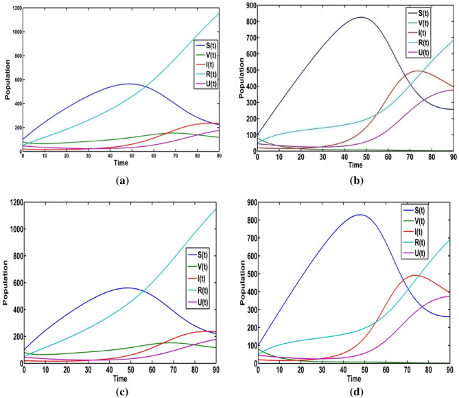
The population trajectories of the crisp model (1) are presented with optimal control, without optimal control, with ${v_1}^{\ast },$ when $v_2=0$ and with ${v_2}^{\ast },$ when $v_1=0$ in Fig. 2.

Fig. 2.

Population trajectories for the crisp system (1) a with optimal control b without optimal control c with ${v_1}^{\ast },$ when $v_2=0$ d with ${v_2}^{\ast },$ when $v_1=0$

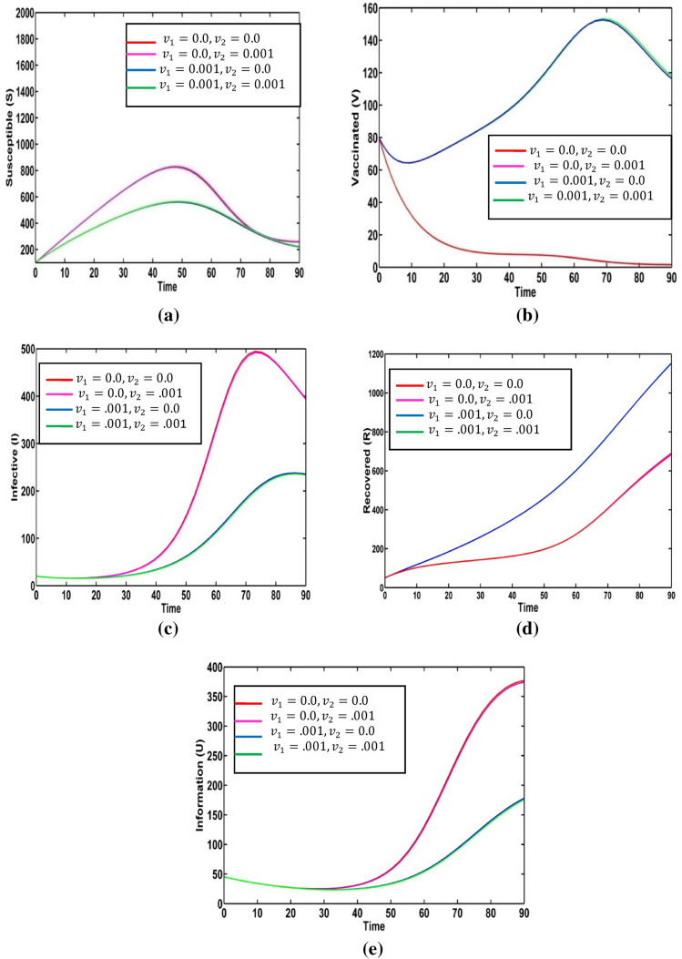
We solve the optimality control system under the optimal values ${v_1}^{\ast },$ ${v_2}^{\ast }$ of the control variables (see Fig. 3). The infective population increases after 30 days and it reaches to the maximum peak between 70 to 80 days for $v_1=0,v_2=0$. So, the disease outbreak is adopted between 70 to 80 days (see Fig. 3c). For control parameter $v_2=0$ and $v_1=0.001,$ vaccinated population is growing up. From the Fig. 3(d), it is seen that the recovered population increases highly for the control variables $v_1=0,v_2=0$. Again, we solve the optimality system for information induced vaccination policy ${v_1}^{\ast }$ and $v_2=0$ (see Fig. 3e). The maximum peak of the information level with controls is less than that of without controls.

Fig. 3.

a Various profiles of susceptible population under ${v_1}^{\ast },$ ${v_2}^{\ast }$. b Various profiles of vaccinated population under ${v_1}^{\ast },$ ${v_2}^{\ast }.$ c Various profiles of infective population under ${v_1}^{\ast },$ ${v_2}^{\ast }.$ d Various profiles of recovered population under ${v_1}^{\ast },$ ${v_2}^{\ast }.$ e Various profiles of information level under ${v_1}^{\ast },$ ${v_2}^{\ast }$

Result 2: Fuzzy model

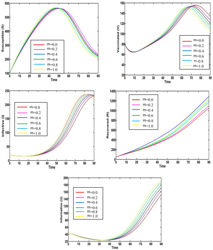
We take the fuzzified values of the fuzzy parameter in terms of triangular fuzzy numbers given in Table 2. We plot variation graphs for different values of degrees of optimism m. Figure 4 presents the variation of susceptible, vaccinated, infective, recovered populations and information level for the different values of degrees of optimism m in fuzzy environment. Here, red, magenta pink, blue, green, cyan and yellow colored lines indicate the populations at $m=0,m=0.2,m=0.4,m=0.6,m=0.8,m=1.0$ respectively. For different values of degrees of optimism $m$, we observe the significant change on the population curves.

Table 2.

Fuzzy parameters and their values

Parameters	TFN
$\tilde{\mathrm{\Pi }}$	$\left(16,20,24\right)$
$\tilde{\lambda }$	$\left(1.6\times {10}^{-4},2\times {10}^{-4},2.4\times {10}^{-4}\right)$
$\tilde{d}$	$\left(3.2\times {10}^{-5},4\times {10}^{-5},4.8\times {10}^{-5}\right)$
$\widetilde{q_0}$	$\left(8\times {10}^{-4},1\times {10}^{-3},1.2\times {10}^{-3}\right)$
$\widetilde{v_1}$	$\left(8\times {10}^{-4},1\times {10}^{-3},1.2\times {10}^{-3}\right)$
$\widetilde{{\theta }_1}$	($8\times {10}^{-3},1\times {10}^{-2},1.2\times {10}^{-2}$)
$\widetilde{{\gamma }_0}$	($8\times {10}^{-4},1\times {10}^{-3},1.2\times {10}^{-3}$)
$\tilde{\psi }$	(0.04, 0.05, 0.06)
$\tilde{\beta }$	(0.0744, 0.093, 0.1116)
$\tilde{\gamma }$	(0.024, 0.03, 0.036)
$\tilde{\delta }$	(0.032, 0.04, 0.048)
$\widetilde{v_2}$	$\left(8\times {10}^{-4},1\times {10}^{-3},1.2\times {10}^{-3}\right)$
$\tilde{b}$	$\left(0.6,0.75,0.9\right)$
$\tilde{g}$	$\left(0.04,0.05,0.06\right)$
$\tilde{a}$	$\left(0.0008,0.001,0.0012\right)$
$\widetilde{p_0}$	(0.04, 0.05, 0.06)

Fig. 4.

Solution trajectories for fuzzy model (2) for the various values of degrees of optimism $m$

Sensitivity of the degradation rate for information ($p_0)$: when $b=0$, ${\theta }_1=0$ and $p_0\in [0.0001,0.5]$

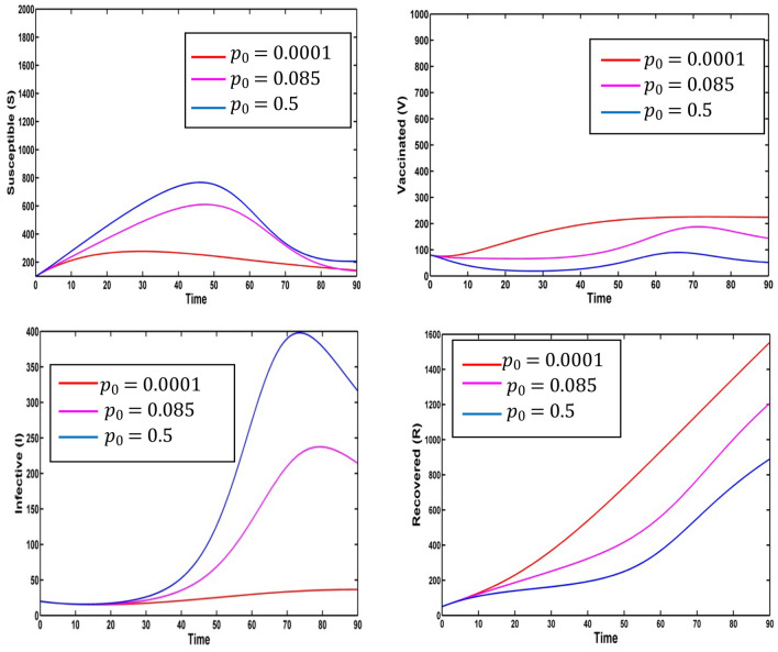
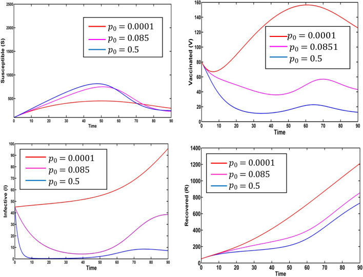
From the model (1), we draw the profiles of the populations for different values of degradation rate for information, $p_0\in \left[0.0001,,,0.5\right]$ (see Fig. 5). When saturation constant for information ${\theta }_1=0$ and rate constant of effectiveness due to treatment $b=0,$ the susceptible population is proportional to the degradation rate for information $p_0.$ The susceptible population increases as the value of $p_0$ increases. The reverse scenario is observed for the vaccinated population. The peak of infection highly increases during 60 days to 70 days for$b=0$, ${\theta }_1=0$ and $p_0=0.5$. Comparatively, it is not higher for the value $p_0=0.085$ for the infective population. For the recovered population, we notice that these populations are inversely proportional to the values of $p_0.$

Fig. 5.

Outlines of population for the various values of $p_0$

Sensitivity of the degradation rate for information ($p_0)$: when $b=0,v_2=0$ (absence of treatment)

When the rate of effectiveness due to treatment $b=0$ and the treatment related control variable $v_2=0,$ we draw the profiles of the populations for different values of $p_0$ (Fig. 6). Susceptible population is proportional to the degradation rate for information $(p_0).$ We observe the reverse scenario for the vaccinated population. The infective population gradually increases for the decrease of the parameter $p_0.$

Fig. 6.

Outlines of populations for the various values of $p_0$

Some numerical results with control policies

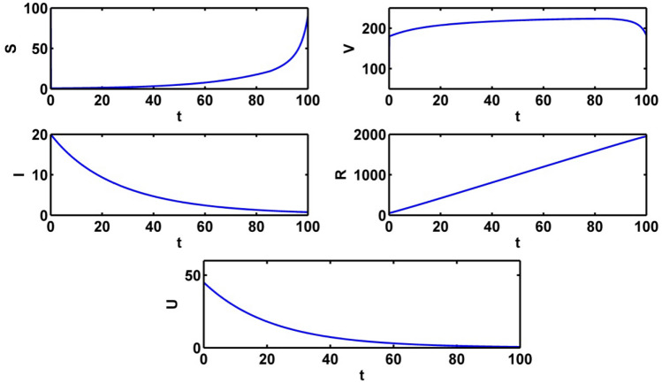
Some numerical results of the crisp model (1) are obtained with control policies. We implement the different control strategies to shorten the disease load and to minimize the total cost with the help of optimal control paths. We consider $v_1$ and $v_2$ as the control variables and take $k_1=1.5,k_2=10,k_3=25$ as positive weight constants. Other parameters values are given in the above Table 1. We analyze the profiles of the populations and minimize the cost for effecting of the implementation of one or both control policies. With the help of MATLAB, the numerical experiments for all the cases are represented. By the forward–backward sweep method, we find the optimal control variables and solve the optimal state system and adjoint state system with respect to time. Figure 7 represents the population trajectories with both control variables and time duration of approximately 100 days. In this case, the recovered population is in its highest level. The susceptible individuals are gradually increased after 40 days. The infective individuals are gradually decreases and it may be diminished after 100 days (approximately). The level of information gradually decreases as time increases.

Fig. 7.

Outlines of populations with both optimal control $v_1^{\ast }$, $v_2^{\ast }$

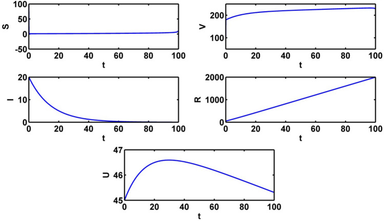
Figure 8 depicts the populations’ profiles when ${v_1=v}_1^{\ast }$ and $v_2=0.$ The level of information increases between 20 to 40 days. There is significant change for the infective population for the presence of optimal control $v_1^{\ast }$, $v_2^{\ast }$ and with only control $v_1^{\ast }$ and $v_2=0.$

Fig. 8.

Outlines of populations with only control $v_1^{\ast }$ and $v_2=0$

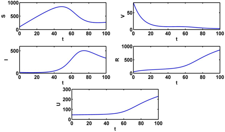
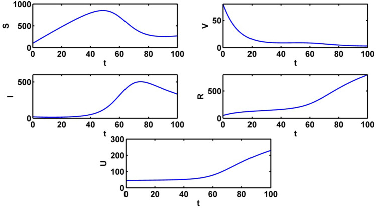
Figure 9 shows the populations’ trajectories in absence of control variables. The susceptible population gradually increases and it reaches to the highest point in about 50 days. Then the curve gradually decreases. At first the infected population is at equilibrium level. The infected population reaches to the highest peak in about 70 days. The intensity of information level gradually increases when no control is applied. We see a significant change for all the population for only control $v_1^{\ast }$ and $v_2=0$ and in absence of control variables.

Fig. 9.

Outlines of populations without optimal control variables

Figure 10 represents the profiles of populations with only control $v_2^{\ast }$ and$v_1=0$. Same scenario is seen in the absence of $v_1^{\ast }$, $v_2^{\ast }$ and also $v_2^{\ast }$,$v_1=0$.

Fig. 10.

Outlines of populations with only control $v_2^{\ast }$ and $v_1=0$

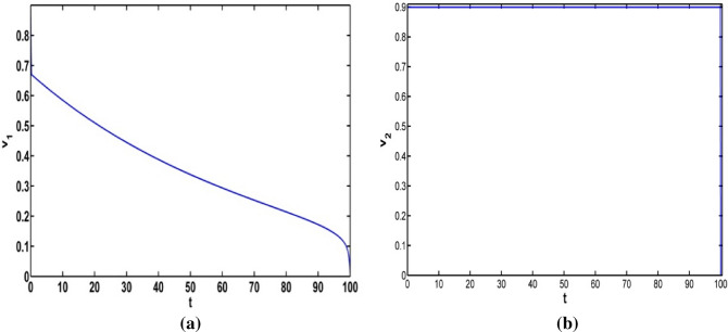
Figure 11a represents the path of the optimal intensity of information related vaccination $v_1^{\ast }$ when $v_2=0.$ Fig. 11b presents optimal control $v_2^{\ast }$ only and $v_1=0.$ From the Fig. 11a, the intensity of control variable decreases gradually with time.

Fig. 11.

a Optimal controls $v_1^{\ast }$ only and $v_2=0.$ b Optimal control $v_2^{\ast }$ only and $v_1=0$

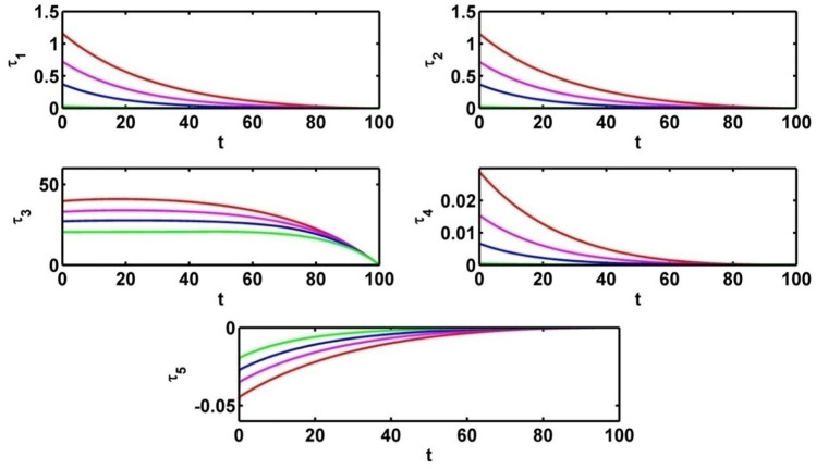
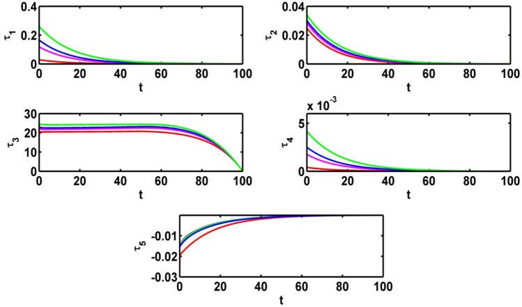
Figure 12 depicts the effect of infected population and level of information for different values of the parameter $\psi$ (vaccine working efficiency)$.$ Using the parameter values in Table 1, we draw the Fig. 12 and Fig. 14 for $\psi =0.05$ (red colored line), $\psi =0.25$ (pink colored line), $\psi =0.50$ (blue colored line, $\psi =0.95$ (green colored line). The infective population is inversely proportional to $\psi .$ When the rate of vaccine working efficiency increases the level of infected population decreases. Thus, the people are curable from the infectious disease but the different scenario is seen for the level of information. The level of information increases when the value of vaccine working efficiency $\psi$ decreases.

Fig. 12.

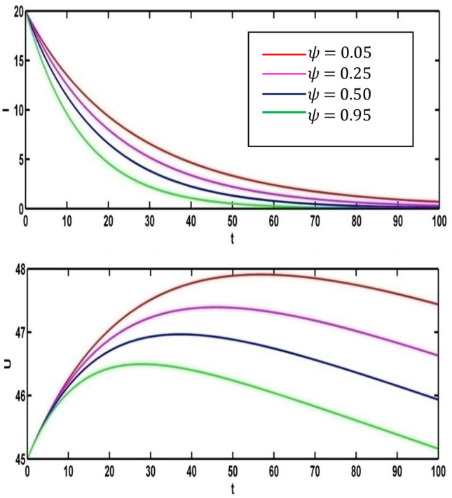
Effect of $\psi$ on infective population and level of information

Fig. 14.

Effect on adjoint variables for various values of $\psi$

Figure 13 represents the effect of control variable for different values of $\psi .$ Fig. 14 depicts the effect on adjoint variables for different values of $\psi$.

Fig. 13.

Effect of control parameters for the various values of $\psi$

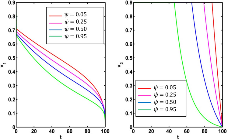
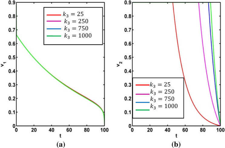
Figure 15 represents the effect on infected population and level of information of the different values of saturation constant for information $({\theta }_1)$. The level of infected population gradually increases as ${\theta }_1$ increases. Again, we plot the level of information for different values of ${\theta }_1$ and see the count of information level increases as saturation constant for information increases. For different values of ${\theta }_1,$ the profile of optimal control and the profile of adjoint variables are presented in Figs. 16 and 17 respectively. Using the values of the parameters in Table 1, we draw the Figs. 16 and 17 for ${\theta }_1=0.01$ (Red colored line), ${\theta }_1=1.0$ (pink colored line), ${\theta }_1=1.5$ (blue colored line) and ${\theta }_1=2.5$ (green colored line).

Fig. 15.

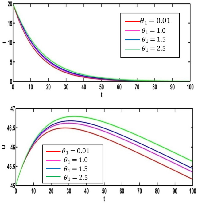
Effect of ${\theta }_1$ on infected population and level of information

Fig. 16.

Profile of optimal control $v_1^{\ast }$ and $v_2^{\ast }$ for various values of ${\theta }_1$

Fig. 17.

Profile of adjoint variables for various values of ${\theta }_1$

Effects of weight constants $k_2,k_3$ on optimal control strategy

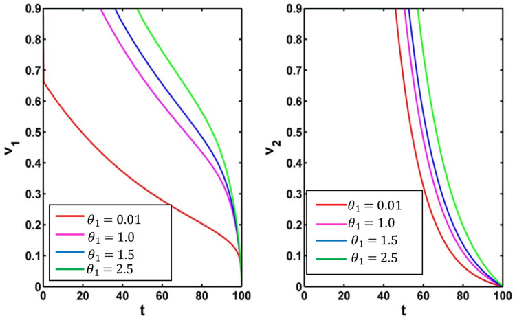
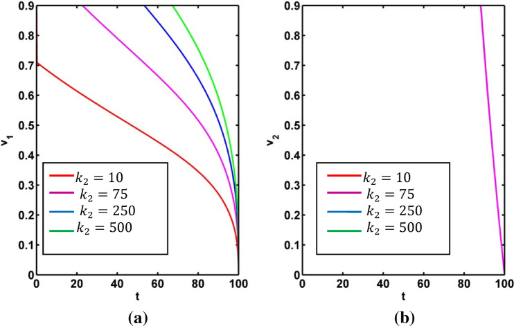
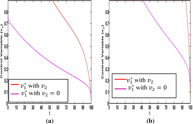
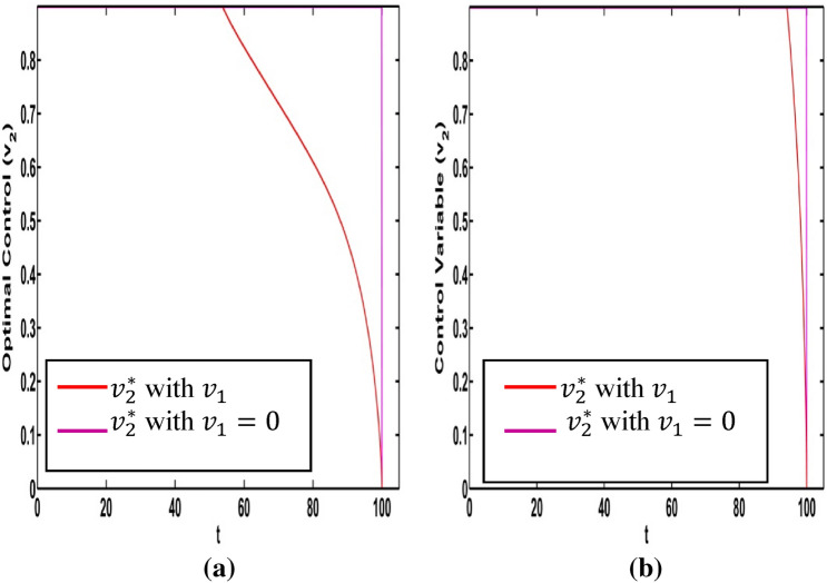
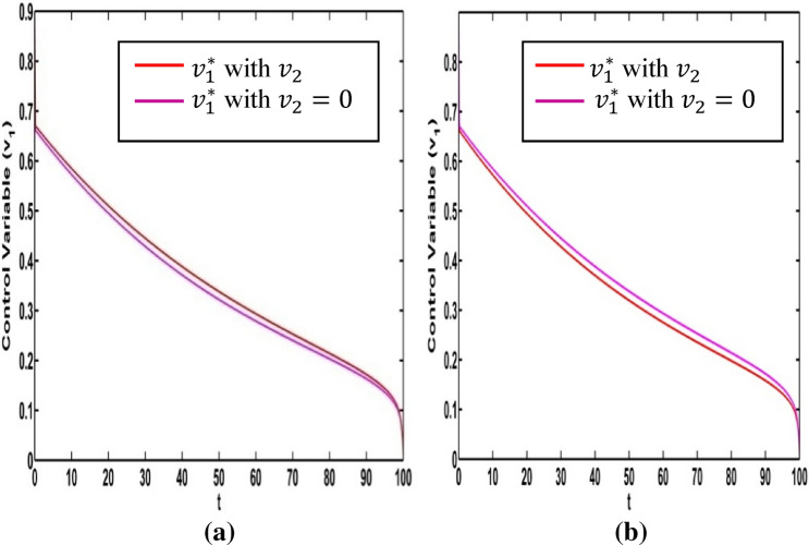
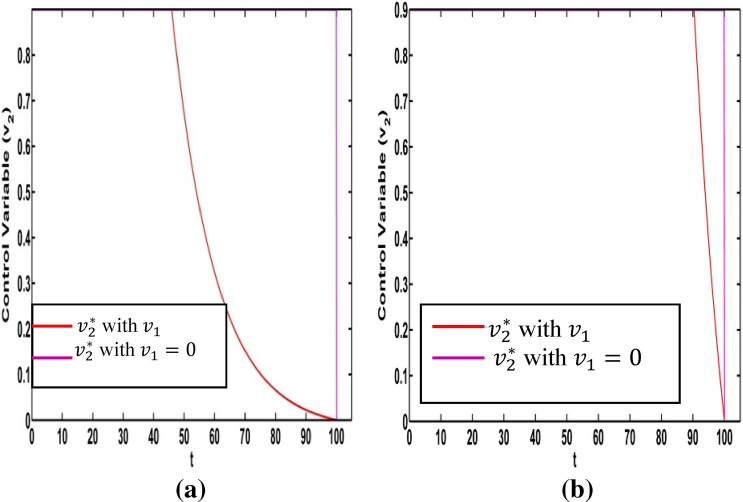
It is very important to discuss the effects of the weight constants on the optimal control for the crisp model (1). We vary the weight constants $k_2,k_3$ while the other parameters are kept fixed. These values are given in Table 1. We change the weight constant $k_2$ and the corresponding profile of optimal control $v_1^{\ast }$, $v_2^{\ast }$ are drawn in Fig. 18a, b. From Fig. 18a it is seen that the optimal control $v_1^{\ast }$ is influenced by weight constant $k_2$ but there is no significant impact for optimal control $v_2^{\ast }$ in Fig. 18b. If the weight constant $k_2=15$ i.e. the vaccination coverage is minimum, the disease transmission is minimized for low strength on information related vaccination $v_1^{\ast }$ ($v_2=0)$ (see Fig. 19a). When the weight constant of vaccination coverage is high ($k_2=750)$, the information related vaccination $v_1^{\ast }$ ($v_2=0)$ is extended for higher intensity (see Fig. 19a). The red and pink colour curves represent the information related vaccintion corresponding to $v_1^{\ast }$ with $v_2$ and $v_1^{\ast }$ with $v_2=0$ respectively. Similar color has been used for $k_2=750$ (see Fig. 19b). There is significant change of $k_2$ for the control $v_2^{\ast }.$ We draw the figure on optimal control $v_1^{\ast }$ and $v_2^{\ast }$ for different values of $k_2.$ From Fig. 20a, b, we observe that optimal control $v_2^{\ast }$ is affected by the weight constant $k_2.$ There is no impact on the optimal control $v_1^{\ast }$ of the weight constant $k_3$ (see Fig. 21a). Figure 21b represents the optimal control $v_2^{\ast }$ for different values of the weight constant $k_3.$ Fig. 22a, b and Fig. 23a, b depict the optimal control $v_1^{\ast }$ for $k_3=25,$ $k_3=1250$, with $k_1=1.5$ and $k_2=10$. From these figures, it is concluded that both the control policies are able to control the disease load and to reduce the economic load at the time of epidemic.

Fig. 18.

a Optimal control $v_1^{\ast }$ for different weight constant $k_2$. b Optimal control $v_2^{\ast }$ for different weight constant $k_2$

Fig. 19.

Optimal control $v_1^{\ast }$ for a $k_2=15$ b $k_2=750$

Fig. 20.

Optimal control $v_2^{\ast }$ for a $k_2=15$ b $k_2=750$

Fig. 21.

a Optimal control $v_1^{\ast }$ for different weight constant $k_3.$ b Optimal control $v_2^{\ast }$ for different weight constant $k_3$

Fig. 22.

Optimal control $v_1^{\ast }$ for a $k_3=25$ b $k_3=1250$

Fig. 23.

Optimal control $v_2^{\ast }$ for a $k_3=25$ b $k_3=1250$

Conclusions

In this work, we discuss a SVIRUS infectious disease model based on the information related to the vaccination and the treatment taking for control strategies and also analyze the minimization of the total cost and the disease load. Firstly, we formulate a model on information related vaccination and treatment in crisp form. Then the model is tranformed into fuzzy model to incorporate the uncertainty of the parameters. With the help of graded mean integration value (GMIV) method, the fuzzy model is converted the defuzzified one. The positivity, the boundedness and the equilibrium analysis of the crisp model are investigated elaborately. The stability of the infection free equilibrium and the infected equilibrium are discussed. Choosing the suitable Lyapunov function, we look into the global stability of infected equilibrium and with the Pontryagin’s Maximum Principle, the existence of the optimal control of the crisp model is explained and all the notable observations are educed numerically and graphically. We establish the effect of the degradation rate for information $(p_0)$ on the information induced disease model. Finally, we conclude that extensive use of both control strategies is more fruitful for the healing of infective population and minimizes the total cost during disease prevelance. The researchers can apply the optimal control policy in other epidemic models. Also, other types of impreciseness like, interval, stochastic, intuitionistic fuzzy, neutrosophic, etc. can be used to tackle the uncertainty of the models.

Funding

DST-INSPIRE, Govt. of India, Ministry of science & Technology, New Delhi, India (DST/INSPIRE Fellowship/2017/IF170211).

Availability of data and materials

The sources of some data are mentioned and the rest data are hypothetical.

Code availability

Not applicable.

Declarations

Conflict of interest

The authors declare that they have no conflict of interest.

References

- Akdim K, Zetouni AE, Zahid M. The influence of awareness campaigns on the spread of an infectious disease: a qualitative analysis of a fractional epidemic model. Model Earth Syst Environ. 2021 doi: 10.1007/s40808-021-01158-9. [DOI] [PMC free article] [PubMed] [Google Scholar]
- Behncke H. Optimal control of deterministic epidemics. Optim Control Appl Methods. 2000;21(6):269–285. doi: 10.1002/oca.678. [DOI] [Google Scholar]
- Brauer F, Chavez CC. Mathematical models in population biology and epidemiology. Berlin: Springer; 2012. [Google Scholar]
- Buonomo B, d’Onofrio A, Lacitignola D. Globally stable endemicity for infectious diseases with information-related changes in contact patterns. Appl Math Lett. 2012;25:1056–1060. doi: 10.1016/j.aml.2012.03.016. [DOI] [Google Scholar]
- Buonomo B, d’Onofrio A, Lacitignola D. Modeling of pseudo-rational exemption to vaccination for seir diseases. J Math Anal Appl. 2013;404(2):385–398. doi: 10.1016/j.jmaa.2013.02.063. [DOI] [Google Scholar]
- Castillo-Chavez C, Feng Z, Huang W. On the computation of R0 and its role in global stability. Inst Math Appl. 2002;125:229–250. [Google Scholar]
- Chen SH, Hsieh CH. Similarity of generalised fuzzy numbers with graded mean integration representation. Proc Int Fuzzy Syst Assoc World Congr. 1999;2:551–555. [Google Scholar]
- Coddington E, Levinson N. Theory of ordinary differential equations. New York: Tata McGraw-Hill Education; 1955. [Google Scholar]
- d’Onofrio A, Manfredi P, Salinelli E. Vaccinating behaviour, information, and the dynamics of SIR vaccine preventable diseases. Theor Popul Biol. 2007;71(3):301–317. doi: 10.1016/j.tpb.2007.01.001. [DOI] [PubMed] [Google Scholar]
- Das A, Pal M. Modeling and analysis of an imprecise epidemic system with optimal treatment and vaccination control. World Sci Publ Comp. 2018;13(1):1–24. [Google Scholar]
- Das S, Mahato P, Mahato SK. A prey predator model in case of disease transmission via pest in uncertain environment. Differ Equ Dyn Syst. 2020 doi: 10.1007/s12591-020-00551-7. [DOI] [Google Scholar]
- Das S, Mahato P, Mahato SK. Disease control prey–predator model incorporating prey refuge under fuzzy uncertainty. Model Earth Syst Environ. 2020 doi: 10.1007/s40808-020-00892-w. [DOI] [Google Scholar]
- Fleming WH, Rishel RW. Deterministic and stochastic optimal control, vol 1. New York: Springer; 1975. p. 1975.20. [Google Scholar]
- Gaff H, Schaefer E. Optimal control applied to vaccination and treatment strategies for various epidemiological models. Math Biosci Eng. 2009;6(3):469–492. doi: 10.3934/mbe.2009.6.469. [DOI] [PubMed] [Google Scholar]
- Gumel AB, Ruan S. Modelling strategies for controlling SARS outbreaks. Proc R Soc Lond. 2004;271(1554):2223–2232. doi: 10.1098/rspb.2004.2800. [DOI] [PMC free article] [PubMed] [Google Scholar]
- Gupta A, Moyer C, Stern D. The economic impact of quarantine: SARS in Toronto as a case study. J Infect. 2005;50(5):386–393. doi: 10.1016/j.jinf.2004.08.006. [DOI] [PMC free article] [PubMed] [Google Scholar]
- Gupta A, Banerjee S, Das S. Significance of geographical factors to the COVID-19 outbreak in India. Model Earth Syst Environ. 2020;6:2645–2653. doi: 10.1007/s40808-020-00838-2. [DOI] [PMC free article] [PubMed] [Google Scholar]
- Joshi H, Lenhart S, Li M, Wang L. Optimal control methods applied to disease models. Contemp Math. 2006;410:187–208. doi: 10.1090/conm/410/07728. [DOI] [Google Scholar]
- Kassa S, Ouhinou A. The impact of self-protective measures in the optimal interventions for controlling infectious diseases of human population. J Math Biol. 2015;70(1–2):213–236. doi: 10.1007/s00285-014-0761-3. [DOI] [PubMed] [Google Scholar]
- Kumar A, Srivastava PK, Takeuchi Y. Modelling the role of information and limited optimal treatment on disease prevalence. J Theor Biol. 2016;414:103–119. doi: 10.1016/j.jtbi.2016.11.016. [DOI] [PubMed] [Google Scholar]
- Kumar A, Srivastava PK, Dong Y, Takeuchi Y. Optimal control of infectious disease: information-induced vaccination and limited treatment. Phys A. 2019 doi: 10.1016/j.physa.2019.123196. [DOI] [Google Scholar]
- Lenhart S, Workman J. Optimal control applied to biological models, vol 1. London: CRC Press; 2007. [Google Scholar]
- Liu X, Takeuchi Y, Iwami S. SVIR epidemic models with vaccination strategies. J Theor Biol. 2008;253(1):1–11. doi: 10.1016/j.jtbi.2007.10.014. [DOI] [PubMed] [Google Scholar]
- Mahata A, Mondal SP, Ahmadian A, Ismail F, Alam S, Salahshour S. Different solution strategies for solving epidemic model in imprecise environment. Complexity. 2018;2018:1–18. doi: 10.1155/2018/4902142. [DOI] [Google Scholar]
- Misra AK, Sharma A, Shukla JB. Modeling and analysis of effects of awareness programs by media on the spread of infectious diseases. Math Comput Model. 2011;53(5):1221–1228. doi: 10.1016/j.mcm.2010.12.005. [DOI] [Google Scholar]
- Nandi SK, Jana S, Manadal M, Kar TK. Analysis of a fuzzy epidemic model with saturated treatment and disease transmission. Int J Biomath. 2018;11(1):1–18. doi: 10.1142/S179352451850002X. [DOI] [Google Scholar]
- Panja P, Mondal SK, Chattopadhyay J. Dynamical study in fuzzy threshold dynamics of a cholera epidemic model. Fuzzy Inf Eng. 2017;9:381–401. doi: 10.1016/j.fiae.2017.10.001. [DOI] [Google Scholar]
- Pontryagin LS, Boltyanskii VG, Gamkrelidze RV, Mishchenko EF. The mathematical theory of optimal processes. New York: Wiley; 1962. [Google Scholar]
- Raeei MA. Numerical simulation of the force of infection and the typical times of SARS-CoV-2 disease for different location countries. Model Earth Syst Environ. 2020 doi: 10.1007/s40808-020-01075-3. [DOI] [PMC free article] [PubMed] [Google Scholar]
- Roy S, Bhunia GS, Shit PK. Spatial prediction of COVID-19 epidemic using ARIMA techniques in India. Model Earth Syst Environ. 2021;7:1385–1391. doi: 10.1007/s40808-020-00890-y. [DOI] [PMC free article] [PubMed] [Google Scholar]
- Russell S. The economic burden of illness for households in developing countries: a review of studies focusing on malaria, tuberculosis, and human immunodeficiency virus/acquired immunodeficiency syndrome. Am J Trop Med Hyg. 2004;71(2):147–155. doi: 10.4269/ajtmh.2004.71.147. [DOI] [PubMed] [Google Scholar]
- Van den Driessche P, Watmough J. Reproduction numbers and sub-threshold endemic equilibria for compartmental models of disease transmission. Math Biosci. 2002;180(1):29–48. doi: 10.1016/S0025-5564(02)00108-6. [DOI] [PubMed] [Google Scholar]
- Zadeh LA. Fuzzy sets. Inf Control. 1965;8:338–353. doi: 10.1016/S0019-9958(65)90241-X. [DOI] [Google Scholar]
- Zaman G, Han Kang Y, Jung I. Stability analysis and optimal vaccination of an SIR epidemic model. BioSystems. 2008;93(3):240–249. doi: 10.1016/j.biosystems.2008.05.004. [DOI] [PubMed] [Google Scholar]
- Zhang X, Liu X. Backward bifurcation of an epidemic model with saturated treatment function. J Math Anal Appl. 2008;348(1):433–443. doi: 10.1016/j.jmaa.2008.07.042. [DOI] [Google Scholar]
Associated Data
This section collects any data citations, data availability statements, or supplementary materials included in this article.
Data Availability Statement