Suspect screening and prioritization of chemicals of concern (COCs) in a forest-water reuse system watershed

Abstract

Much research has assessed organic chemicals of concern (COCs) in municipal wastewater and receiving waters, but few studies have examined COCs in land treatment systems. Many prior studies have implemented targeted methods that quantify a relatively small fraction of COCs present in wastewater and receiving waters. This study used suspect screening to assess chemical features in ground- and surface waters from a watershed where secondary-treated wastewater is irrigated onto 900 ha of temperate forest, offering a more holistic view of chemicals that contribute to the exposome. Chemical features were prioritized by abundance and ToxPi scoring across seasonal sampling events to determine if the forest-water reuse system contributed to the chemical exposome of ground- and surface waters. The number of chemical features detected in wastewater was usually higher than on- and off-site ground- and surface waters; in wastewater, chemical features trended with precipitation in which greater numbers of features were detected in months with low precipitation. The number of chemical features detected in off- and on-site waters was similar. The lower overlap between chemical features found in wastewater and downstream surface waters, along with the similar numbers of features being detected in upstream and downstream surface waters, suggests that though wastewater may be a source of chemicals to ground and surface waters on-site, dissipation of wastewater-derived features (in number and peak area abundance) likely occurs with limited off-site surface water export by the forested land treatment system. Further, the numbers of features detected on site and the overlap between wastewater and surface waters did not increase during periods of low rainfall, counter to our initial expectations. The chemical features tentatively identified in this watershed appear common to features identified in other studies, warranting further examination on the potential for resulting impacts of these on humans and the environment.

Graphical Abstract

1. Introduction

Forested land application systems, also known as forest-water reuse systems, involve the application of municipal wastewater (untreated or treated) to forested lands. This results in slow-rate soil infiltration to groundwater recharge and finally surface water discharge, serving as an active component of water treatment and management (Crites, 1984). When appropriately managed, these systems can offer a favorable means of delivering sustainable water while preserving forested habitats and the ecosystem services therein (Bastian, 2005; Crohn, 1995; Magesan and Wang, 2003; Nichols, 2016).

While much is known about the functioning of these systems in terms of nutrient and micronutrient removal (Nichols, 2016 and references therein), fewer studies have assessed the environmental fate of organic chemical contaminants of concern (“COCs”) in these particular wastewater treatment systems. COCs are a growing concern for managing for sustainable public water and waste/sanitation hygiene systems (Benson et al., 2017; Clarke and Smith, 2011; Pereira et al., 2015). Organic COCs consist of legacy contaminants (e.g. polycyclic aromatic hydrocarbons “PAHs”, polychlorinated biphenyls “PCBs”, legacy pesticides including DDT, etc.) and contaminants of emerging concern, or “CECs.” A CEC is defined by Diamond et al. (2011) as one of over 40,000 organic contaminants for which “there are increasing concerns regarding its potential risks to humans and ecological systems,” and include pharmaceuticals, disinfection by-products, endocrine disrupting compounds, plasticizers, surfactants, flame retardants, pesticides, high production volume chemicals, and their degradates. COCs are commonly detected in wastewater and subsequently, in receiving waters and soils of wastewater effluent (Cincinelli et al., 2012; Harrison et al., 2006; Hedgespeth et al., 2012; Köck-schulmeyer et al., 2013; Lampard et al., 2010; Sedlak et al., 2008).

Previously, researchers have called for field-scale studies on the environmental impacts of land application due to increased pressures for water reuse (O’Connor et al., 2004). Studies to date, however, have primarily focused on the fate of COCs in biosolids and reclaimed water application to agricultural lands, as well as COC uptake by food crops (Gushit et al., 2013; Kipopoulou et al., 1999; Riemenschneider et al., 2016; Wu et al., 2015). A few studies have assessed COCs within land application systems and found that land applied wastewater contributed to the presence of chemicals in ground- and surface waters (Karnjanapiboonwong et al., 2011; Kibuye et al., 2019; Lesser et al., 2018; McEachran et al., 2016, McEachran et al., 2017a).

Most studies assess the presence of COCs in wastewater and environmental samples using targeted approaches wherein specific chemical/s are identified a priori and quantified with authentic analytical standards (Cahill et al., 2004; Cincinelli et al., 2012; Köck-schulmeyer et al., 2013; Lesser et al., 2018; Scheurer et al., 2011). “Non-targeted” or “untargeted” analytical approaches, such as suspect screening and non-targeted analyses, screen for a broader range of chemicals not decided upon a priori and are increasingly used to screen for COCs in environmental samples (Gosetti et al., 2016; Hollender et al., 2017). Both approaches involve the use of high-resolution mass spectrometry (HRMS) for the chemical analysis of environmental samples. The spectral output of suspect screening analysis is compared with compound-specific parameters available in chemical databases as a means to tentatively identify chemicals present in the samples. In non-targeted analysis, no a priori information is available. Chemical identities can subsequently be confirmed and quantified using suspect screening and non-targeted approaches if reference standards are available. These approaches have been used for the analysis of pharmaceutical metabolites in wastewater influent (Gago-Ferrero et al., 2015), detection of novel micropollutants in wastewater effluent (Hug et al., 2014), and assessment of chemical removal at different stages of the wastewater treatment process (Nürenberg et al., 2015). Non-targeted approaches have also been used to examine samples taken from rivers (Ruff et al., 2015; Strynar et al., 2015) and groundwater (Soulier et al., 2016) impacted by municipal wastewater, industrial wastewater, and/or agricultural land use. To date, there are no comprehensive studies utilizing non-targeted approaches to analyze COCs that may be present in forested land application systems for water reuse.

This study utilized a suspect screening approach to assess organic COCs in a watershed where secondary-treated municipal wastewater is irrigated onto 900 ha of temperate forestland. Quarterly grab samples from irrigated and non-irrigated areas in the watershed were used to evaluate the chemicals that contribute to the “exposome” (Wild, 2005, Wild, 2012) in waters impacted by wastewater irrigation to waters off site. Prior research at this specific site focused primarily on targeted analysis of a subwatershed comprising about 60% of the total forest area and did not extensively evaluate the unknown chemical exposome of groundwater or surface water across the watershed on- and off-site of the facility (Birch et al., 2016; McEachran et al., 2016, McEachran et al., 2017a, McEachran et al., 2018). A hydrological evaluation of the irrigated subwatershed found that groundwater was 50–76% derived from wastewater and that the wastewater fraction in exported surface waters contained 23 to 60% wastewater under normal rainfall and drought conditions, respectively (Birch et al., 2016). Prior targeted studies quantified selected pharmaceuticals and personal care products in waste-, ground-, and surface waters in the same subwatershed (McEachran et al., 2016, McEachran et al., 2017a) and have demonstrated that chemicals were detected at similar or lower concentrations in the surface water outlet of this forested land application system than in receiving surface waters from conventional wastewater treatment (McEachran et al., 2016). Additionally, a limited suspect screening study compared upstream and downstream surface waters from a subwatershed of the forested land treatment site to the surface waters collected at a conventional wastewater treatment plant (McEachran et al., 2018). For the forested site, only 30% of the total number of chemical features in wastewater effluent was detected in the downstream surface water sample.

Therefore, our study provides a more spatially and temporally extensive evaluation using a stratified sampling approach by soil type and catchments and suspect screening analysis of waste-, ground-, and surface waters at the scale of the entire watershed. The use of suspect screening allows for a broader assessment of the chemical exposome across different water types, time points, and spatial locations (on-site irrigation versus off-site, adjacent lands). We expected that wastewater would contribute more chemical features to the chemical exposomes of groundwater and surface water on site than from waters off site. We also expected the number and overlap of chemical features in wastewater to increase in groundwater and surface waters on site during periods of low rainfall. Results of suspect-screening were used to prioritize tentatively identified features to more holistically evaluate potential COC toxicity and exposure to humans and wildlife over time and space, an important aspect of the exposome (Wild, 2005, Wild, 2012). This approach not only addresses unrealized and unknown COCs in the present but supports future studies on chemical features/groups of interest via retrospective analyses.

2. Methods

2.1. Sample site and collection

The City of Jacksonville’s Land Treatment Site (LTS) is a forest-water reuse system that serves approximately 70,000 customers and treats roughly 19 million L municipal wastewater/day; this system has previously been described by Birch et al. (2016) and McEachran et al. (2016). The LTS utilizes secondary treatment and disinfects of the effluent via chlorination prior to irrigation. The site relies on infiltration of water through soil before release to receiving waters, i.e. groundwater and subsequently surface water streams, at the site. Site precipitation and irrigation were calculated based on cumulative precipitation data obtained from on-site rain gauges located near sampling locations and the averaged cumulative irrigation for blocks located near sampling locations. Cumulative daily precipitation and cumulative daily loading (irrigation) were calculated from one previous sampling event to the next.

LTS sampling occurred in August 2017, December 2017, March 2018, and June 2018, and sampling locations selected were stratified based on soil types and irrigation input (Fig. 1). The locations sampled included wastewater effluent (pre- and/or post-chlorination; WW16 and 13, respectively), groundwater samples from an off-site well and a natural spring (R1, GW8), ten wells located throughout irrigated areas of the site for required facility monitoring (GW1, 2, 3, 5, 6, 7, 11, 12, 17), surface water from two streams located upstream of the site in areas that did not receive irrigation (SW18, 19), surface water from streams on site that are within the irrigated area (SW1, 2, 3, 5, 6, 7, 11, 17), and streams downstream of the site in areas that did not receive irrigation (SW14, 15, 16, 20). Wastewater samples were collected from a holding reservoir (pre-chlorination) and a central spigot located between holding reservoirs and the irrigation system (post-chlorination). Groundwater wells were purged three volumes prior to sample collection using a peristaltic pump. Surface water sites were selected in close proximity to groundwater monitoring well locations. All grab samples (500 mL) were collected in glass, amber bottles previously cleaned, rinsed with deionized water, solvent-rinsed using methanol, and dried in an oven at 60 °C, modified from the USGS National Field Manual for the Collection of Water-Quality Data (USGS, 2004). Samples were stored on ice during transport and at 4 °C until extraction in the laboratory (within 72 h after collection).

Figure 1.

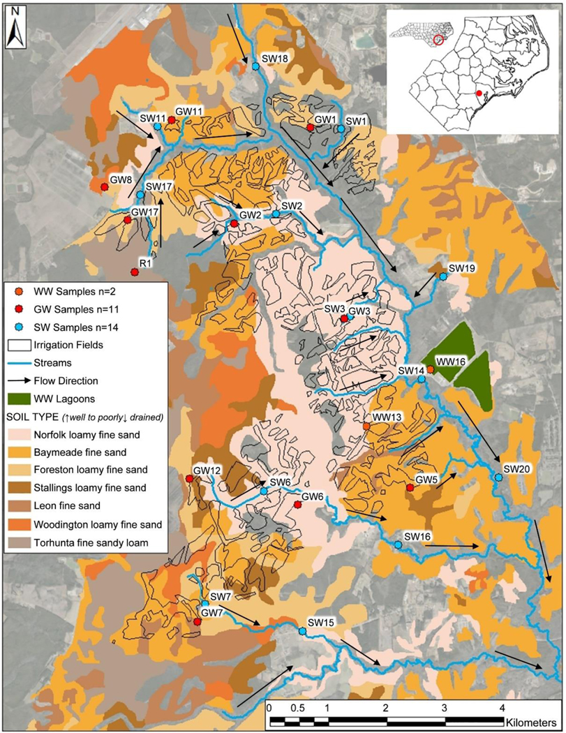
Map of the Jacksonville, NC, Land Treatment Site (LTS) showing wastewater (WW), groundwater (GW), and surface water (SW) sampling locations, along with soil types. Areas outlined in black indicate irrigated regions of the site. Arrows indicate general directional flow of water at the site.

2.2. Sample processing and extraction

Sample processing and extraction followed methods modified from prior studies by McEachran et al. (McEachran et al., 2016, McEachran et al., 2017a). Immediately prior to extraction, the samples were filtered using 9 cm Whatman GF/A filters (1.6 μm pore size) under gentle vacuum using 9 cm porcelain Buchner funnels and glass filter flasks. Each sample was then spiked with isotopically labeled surrogate recovery standards (Table A.1) and weighed prior to extraction. Standards were chosen based on environmental presence (McEachran et al., 2017a), and to reflect a broad range of classes/uses as well as predicted logP values, or XlogP3 (Cheng et al., 2007), i.e. of matched unlabeled chemicals which they represent.

Solid phase extraction (SPE) of the samples occurred by loading onto 6 cc/500 mg Oasis HLB cartridges (60 μm particle size) at a flow rate of 10 mL/min after first conditioning cartridges with methanol, then deionized water. Once samples were fully loaded, containers were re-weighed to determine the volume of sample extracted. Cartridges were then dried under vacuum for 15 min, followed by washing with 2 mL deionized water, then dried again for 15 min. A set of five 15 mL Falcon tubes were weighed to determine average weight and cartridges were then eluted using 10 mL of methanol. Eluents were re-weighed to determine total volume eluted, vortexed, and then extracts split; 4 mL of extract was transferred to amber glass vials for analyses using GC–MS (gas chromatography mass spectrometry) in another laboratory (data not reported here).

The remainders of the extracts analyzed for this study were placed under a gentle nitrogen stream in 40 °C water bath and allowed to evaporate until the volume remaining was ≤1 mL. All extracts were brought to 1 mL volume with methanol, vortexed, and then centrifuged at 10000 RPM for 5 min to remove potential particles that may have formed during evaporation. Extracts were then transferred to amber, glass autosampler vials (950 μL of extract) and stored at −80 °C until analysis. Immediately prior to analysis, 30 μL of extracts plus 270 μL of ammonium acetate buffer solution (2 mM in deionized water) were transferred to separate autosampler vials for instrumental analysis.

2.3. Instrumental analysis

High performance liquid chromatography (HPLC) time-of-flight high resolution mass spectrometry (TOF-HRMS) was carried out using an Agilent 1100 HPLC interfaced with an Agilent 6210 TOF-HRMS. A Waters Cortecs T3 column (3 mm × 100 mm, 120 Å, 2.7 μm) was used for chromatographic separation, for which the method consisted of the following conditions: 0.3 mL/min flow rate; column held at 30 °C; mobile phase A: ammonium formate buffer (0.4 mM) and DI water:methanol (95:5 v/v), and mobile phase B: ammonium formate (0.4 mM) and methanol:DI water (95,5 v/v); gradient: 0˗3 min linear gradient from 90:10 A:B to 75:25 A:B; 3˗10 min linear gradient from 75:25 A:B to 20:80 A:B; 10˗13 min linear gradient from 20:80 A:B to 100% B; 13˗14 min hold at 100% B. The TOF-HRMS was operated in both ESI-negative and ESI-positive ionization modes using a separate injection for each mode and a fragmentor voltage of 125 V. Data were collected in 4 GHz high resolution mode, collecting ions in 100–1700 m/z range in both centroid and profile data formats.

2.4. Data processing

Molecular features were extracted and aligned using Profinder in Agilent MassHunter Workstation Software (v. B.08.00). The feature extraction and alignment methods used were based on user-specified criteria similar to those in an initial suspect screening of LTS samples (McEachran et al., 2018) with some modifications. Background noise thresholds were set to 1000 counts and molecular feature extraction filters were set to 5000 counts with ion-EIC peak and ion post-processing filters set to 3000 counts. Retention windows of 0.4 min and mass windows of 20 ppm ± 2.00 mDa were set as inter-sample feature alignment thresholds. These settings were used for data collected in both ESI-positive and ESI-negative modes and across all sampling events. Features were then matched to chemical formulae contained in the USEPA’s Distributed Structure-Searchable Toxicity database (DSSTox, v. 12/2016) which contained 142,507 unique molecular formulae corresponding to ~765,000 chemical substances. Matching was performed using Agilent Mass Profiler Professional, for which matches were scored based on neutral accurate mass, isotope distribution, and isotope ratio.

All features were then run through additional data processing using R (v. 3.5.1; R Core Team, 2013) for additional filtering – peaks in samples with areas which were <3 times the peak areas in field blanks were removed and duplicate chemical features with the same masses and retention times were collapsed to a single identification. The use of single MS in this study results in the identification of unequivocal molecular formulae for features with a ≥90% match score, i.e. resulting in an identification confidence of Level 4 according to Schymanski et al. (2014). We have termed these “tentative knowns.”

Though MS/MS data were not obtained, we assigned tentative candidate structures to unequivocal formulae (only those features with a ≥90% match score) by performing a batch search of the MS-ready formulae using the USEPA’s CompTox Chemicals Dashboard (https://comptox.epa.gov/dashboard; retrieved 08/2018; Williams et al., 2017) for which the top most likely candidate was retrieved based on the largest number of data sources (McEachran et al., 2017b), i.e. termed “tentatively identified feature” (refer to Figs. A.1–A.5 for an example). In some cases, more than one top candidate was found for a single formula, therefore all top candidates for those formulae remained in the final dataset. Additional data on these tentatively identified features were also retrieved from the CompTox Dashboard including identifiers, intrinsic and predicted properties, and other metadata. In order to determine chemical use categories for the tentatively identified features, features were matched against the two following databases. CASRNs of features were matched against the USEPA iCSS ToxCast Dashboard (https://actor.epa.gov/dashboard/; retrieved 11/21/2018) for retrieval of CPCat data on use categories (also available from https://actor.epa.gov/cpcat/faces/home.xhtml; Dionisio et al., 2015). DTXSIDs of the features were run against a downloadable version of the USEPA’s CPDat database (v 1.0, 10/5/2016) available on the CompTox Dashboard for retrieval of functional use data (Dionisio et al., 2018).

To enable prioritization of tentatively identified features, ToxPi scores were calculated according to Rager et al. (2016) using metadata pulled from the CompTox Dashboard; however, subscore components were equally weighted as performed by Newton et al. (2018). Stated briefly, ToxPi scores were calculated for each tentatively identified feature (i) using its bioactivity (B) ratio, exposure category (E), detection frequency (DF), and abundance based on average chromatographic peak area (A), according to Eq. (1), for which E, DF, and A values were log-transformed before applying Eq. (1).

$$\text{ToxPi}\text{Score}=\frac{{\text{B}}_i-{\text{B}}_{\min }}{{\text{B}}_{\max }-{\text{B}}_{\min }}+\frac{{\text{E}}_i-{\text{E}}_{\min }}{{\text{E}}_{\max }-{\text{E}}_{\min }}+\frac{{\text{DF}}_i-{\text{DF}}_{\min }}{{\text{DF}}_{\max }-{\text{DF}}_{\min }}+\frac{{\text{A}}_i-{\text{A}}_{\text{min}}}{{\text{A}}_{\max }-{\text{A}}_{\min }}$$ (1)

2.5. Quality assurance and quality control

Both field and analytical quality control measures were implemented during each sampling event. A field blank comprised of HPLC water and a laboratory blank comprised of deionized water were analyzed with each sample set. Overall 424 ± 98 features (mean ± one standard deviation) were detected in field blanks prior to the data filtering step of the workflow (i.e. field blank subtraction, removal of duplicates, etc. in R; Table A.2). Field duplicate grab samples of one ground- and one surface water site were collected during each sampling event (site location was chosen randomly at the time of sampling) to determine precision of methods beginning from field sampling through the suspect screening analysis workflow. Precision for the entire study based on match percentage averaged 91 ± 3.2% (Table A.2). Average responses (peak areas) and variability therein (residual standard deviation) were determined for the isotopically labeled surrogate recovery standards spiked into samples with RSDs ranging from 10 to 45%. These, along with retention time drift, are reported in Table A.3. During instrumental analysis, methanol blanks were run intermittently to reduce potential carryover and served as solvent blanks. Any drift in mass accuracy of the instrument was continuously corrected for via infusion of the two reference compounds purine and hexakis (1H, 1H, 3H-tetrafluoropropoxy) phosphazene.

2.6. Data analysis

Abundances (peak areas) of chemical features contributing to ≥1% of total abundance for each sampling event were statistically compared using Wilcoxon rank−signed tests (residuals of the data using parametric tests were not normally distributed). These analyses compared the following site types: on- vs. off-site groundwater, on- vs. off-site surface water (upstream or downstream), and off-site upstream vs. downstream surface water. For each test, the abundances of the same chemical features detected in the two site types were compared in a pairwise fashion for each feature. To account for the multiple comparisons run for surface water samples (i.e. 3 tests per sampling event), α was adjusted to 0.0167 using Bonferroni correction (Bonferroni, 1936).

3. Results & discussion

3.1. Chemical features linked to rainfall, irrigation, and soil types

The Jacksonville LTS demonstrates a general northwestern to southeastern hydraulic gradient for both ground and surface waters in the watershed (Fig. 1). Therefore, off-site surface waters were sampled upstream (north) and downstream (south) of the site, and off-site groundwater was sampled from the northwestern region of the site. Our primary hypotheses were as follows: 1.) wastewater would contribute more chemical features to the chemical signature of groundwater and surface water on site than from waters off site; and 2.) the number and overlap of chemical features in wastewater would increase in groundwater and surface waters on site during periods of low rainfall.

In line with our first hypothesis, wastewater effluent usually contained the greatest numbers of chemical features (based on accurate mass, retention time, and integrated abundance) compared to surface water and groundwater samples on and off site of the irrigated facility boundaries (Fig. 2 a & b, Table A.4). Other studies have observed more features for wastewater effluent than surface waters upstream and downstream of wastewater release (McEachran et al., 2018; Pochodylo and Helbling, 2017). The exception to this trend in this study was the August sampling event for which groundwater (Fig. 2 a) as well as on- and off-site downstream surface water (Fig. 2 b) contained similar numbers of chemical features as wastewater. For the June event, off-site groundwater also contained similar numbers of features as wastewater (Fig. 2 a). The number of chemical features detected in wastewater effluent tended to vary inversely with precipitation (Fig. 2) wherein more chemical features were detected in wastewater during low precipitation periods (March) and fewer features were observed when precipitation was high (August), likely due to dilution in lagoons. Both pre- and post-chlorinated wastewater effluent contained similar numbers of features for the two events in which both samples were collected (Table A.4).

Figure 2.

Mean number of chemical features detected in wastewater effluent and a.) groundwater and b.) surface waters, along with c.) cumulative precipitation and irrigation for each sampling event. Error bars represent the mean ± one standard deviation.

Heavy precipitation may result in increased input of polar organic chemicals into surface waters due to unintentional discharge of untreated wastewater when wastewater storage capacity is exceeded (Buerge et al., 2003). This scenario does not apply to this facility because of the large storage capacity in lagoons, preventing overflowing. However, the large numbers of chemical features detected in groundwater and downstream surface waters seen in the August sampling event in this study may also be due to lower residence times during treatment (Buerge et al., 2003) or the “flushing” of chemicals from groundwater or soils during heavy precipitation events (McEachran et al., 2017a).

The numbers of chemical features detected in groundwater and surface waters were similar to one another (Fig. 2 a & b, Table A.4), as were the numbers of chemical features detected for on-site and off-site groundwater and surface waters. Counter to our second hypothesis, we did not see an increase in numbers of features detected in on-site ground- or surface waters in March, i.e. the sampling event associated with the lowest amount of rainfall (Fig. 2). However, more features were detected in off-site groundwater than on-site groundwater for the March sampling event. Additionally, off-site groundwater samples showed the greatest variability in number of features detected. Temporal factors, such as seasonal agricultural practices near the off-site groundwater sampling locations, may explain this occurrence. The numbers of chemical features for on- and off-site groundwater appear to be inversely related to irrigation, i.e. fewer numbers of features were detected when irrigation was higher and vice versa (Fig. 2 a & c). We suspect that factors including differences in soil drainage (Fig. 3, Table A.4) likely play a large role in chemical feature detection in groundwater. For example, more chemical features were detected in areas with slower draining soils, with off-site groundwater samples collected from the poorest draining soils (Fig. 3, Table A.4).

Figure 3.

Box-and-whisker plot of numbers of chemical features detected in groundwater samples across sampling events based on soil type with a description of soil drainage ranging from “well-drained” to “very poor drainage.”

The numbers of chemical features in surface water entering the site watershed were similar to the numbers of chemical features in surface waters downstream of the land treatment system except for August 2018 (Fig. 2 b). In August, downstream surface waters contained more chemical features than upstream locations; however, only one upstream location was sampled that month. Generally, the numbers of features in off-site upstream samples inversely trend with precipitation. On-site surface water samples demonstrated the greatest number of features detected in December, which may be linked to high irrigation, though numbers of chemical features detected in on-site surface water locations appear relatively stable. Numbers of features in off-site downstream locations trend inversely with irrigation, and these trends appear similar to groundwater samples. Off-site downstream surface water samples demonstrated the greatest number of chemical features detected in the August sampling event (also the case for on-site groundwater samples), which may reflect high precipitation.

Total abundances (i.e. peak areas) of chemical features detected for this study were also compared. Abundance can roughly be correlated to the total “concentration” of all chemical features detected in the sample set for a given event, though abundance is only relative to other masses in the sample. Abundance is not meant to serve as a direct proxy of chemical concentration; interpretations of results based on abundance should therefore be performed with caution. Differences in ionization efficiencies can result in up to 6-fold variability in peak areas, which may be impacted by LC solvents used, compound properties, and matrix effects (reviewed by Kruve, 2018). However, we argue that it is also important to consider the abundances (i.e. peak area) of features detected for a sampling event since relatively few features may make up a large proportion of the total abundance, i.e. a large proportion of the chemical signature.

Abundances of chemical features contributing to ≥1% of total abundance were statistically compared in on- vs. off-site groundwater for each sampling event in a pairwise fashion for each feature (Table 1). As mentioned previously, greater numbers of features were detected in off-site groundwater than on-site groundwater for March and off-site groundwater showed the greatest variability in number of features detected (Fig. 2 a). However, the abundances of features in on-site groundwater were significantly greater than those found in off-site groundwater (except for the March 2017 sampling event) even though the numbers of features detected were similar. For March, abundances were not significantly different in groundwater found on and off site (Table 1). The same pairwise analyses on abundance were performed for surface water on and off site, including an additional comparison of upstream vs. downstream samples collected off site (Table 1). Similar to groundwater, abundances were also significantly greater in on-site vs. off-site upstream surface waters in all events except for March 2017. When comparing on-site vs. off-site downstream surface waters, abundances on site were significantly larger in December 2017 and June 2018 only. Abundances were also significantly larger in off-site downstream vs. off-site upstream surface waters in August 2017 (where greater numbers of features were also detected downstream) and June 2018. For the March 2017 sampling event, i.e. the event receiving the lowest precipitation and irrigation (Fig. 2 c), all pairwise abundance comparisons were similar.

Table 1.

Wilcoxon rank−signed test results of comparisons of peak area abundance of chemical features (n) making up ≥1% of total abundance for each sampling event. Pairwise tests compared off- and on-site ground or surface waters for each sampling event. For surface water comparisons, α was adjusted using Bonferroni correction. Significant differences between site types are indicated in bold.

		GW	SW (α = 0.0167)
		On site vs. off site	On site vs. off site (upstream)	On site vs. off site (downstream)	Off site (upstream) vs. off site (downstream)
Aug. 17 n = 20	p-Value	p < .001	p < .001	0.96	p < .001
	Z score	−5.83	−4.76	−0.0548	−3.80
Dec. 17 n = 25	p-Value	p < .001	p < .001	p < .001	0.237
	Z score	−3.79	−4.76	−4.70	−1.18
Mar. 18 n = 14	p-Value	0.124	0.0310	0.0254	0.0653
	Z score	−1.54	−2.16	−2.24	−1.84
Jun. 18 n = 21	p-Value	0.004	0.003	0.004	0.004
	Z score	−2.90	−2.96	−2.87	−2.87

3.2. Wastewater contribution to ground- and surface waters

Other studies using nontargeted approaches have found greater numbers and/or concentrations (or abundances) of chemicals in groundwater (Soulier et al., 2016) and rivers (Ruff et al., 2015; Strynar et al., 2015) sampled downstream of point and non-point sources, i.e. municipal wastewater, industrial wastewater, and/or agricultural land use. Wastewater input did not appear to impact on-site groundwater or surface water in terms of raw numbers of features detected in samples in this study. However, pairwise comparisons of peak area abundances on- and off-site indicate that samples collected on site showed larger abundances, or “concentrations,” of the chemical features present in August 2017, December 2017, and June 2018, which may have been a result of wastewater input to groundwater and surface water on the land treatment site. The site received the lowest water input in terms of precipitation and irrigation in March 2017 (Fig. 2 c), likely resulting in the similar on- and off-site abundances seen in our study.

To further examine the potential impact of wastewater on receiving waters, the numbers of identical chemical features found in wastewater vs. on-site groundwater and on-site surface water were compared as a proxy for wastewater contribution to on-site receiving waters. The numbers of identical features present in multiple site types were then calculated relative to the total number of features detected for an individual sampling event, resulting in the percentage of “overlap” (Table 2). Greater percentages of overlap may represent a greater contribution of wastewater to a given receiving water type; however, upstream or off-site sources of chemicals must also be considered. Wastewater’s estimated contribution to on-site groundwater and surface water was highest in December, which is also the period during which the site received the most irrigation (Table 2; Fig. 2 c). Again, abundances were also greater in on- vs. off-site groundwater samples during December, though the numbers of features detected on and off site were similar (Table 1; Fig. 2 a). This was also the month for which the greatest number of features was detected in on-site surface water (Fig. 2 b), and for which abundances were significantly greater in on-site surface water vs. off-site upstream and downstream samples (Table 1). Contrary to our second hypothesis, wastewater’s estimated contribution to on-site groundwater and surface water was lowest in March (Table 2). This month received the lowest amount of irrigation and precipitation (Fig. 2 c) and was the event for which the greatest number of features were detected in wastewater overall (Fig. 2 a). However, abundances of features did not significantly differ in on- and off-site groundwater samples (Table 1) and greater numbers of features were detected off site (Fig. 2 a). For surface waters on and off site, numbers of features (Fig. 2 b) and abundances (Table 1) were similar in March.

Table 2.

“Overlaps” show the percentage of chemical features that are present in wastewater in addition to the other site types as a proxy of relative contribution of wastewater to each site type.

% identical chemical features found in WW versus
	GW off-site	GW on-site	SW off-site upstream	SW on-site	SW off-site downstream
Aug. 17	21	23	14	24	21
Dec. 17	16	24	13	36	18
Mar. 18	18	16	13	19	15
Jun. 18	21	20	13	20	17
Average ± SD	19 ± 2.4	21 ± 3.6	13 ± 0.50	25 ± 7.8	18 ± 2.5

A prior study of a subwatershed of the Jacksonville LTS demonstrated that predicting the wastewater composition of ground- and surface water is complex due to nonlinear processes associated with the soil water balance, but that wastewater composition of surface waters located in irrigated regions tended to increase during periods of low precipitation (Birch et al., 2016). However, our findings are inconsistent with our expectation of wastewater’s greatest contribution of COCs to surface water during the driest sampling event (i.e. March; Fig. 2 c). We did not see an increase in the number of total chemical features detected in on-site streams during the month of March, nor was the overlap in numbers of features detected in waste- and surface waters the greatest for this sampling event (Fig. 2 b; Table 2). Similarly, abundances of features detected in on- and off-site surface waters did not significantly differ for this sampling event (Table 1). Stable isotope analysis would be necessary to confirm whether the actual contribution of wastewater to receiving surface waters during the dry period was in fact lower, or whether the trend seen by Birch et al. (2016) was simply not captured due to the relatively low temporal resolution of this study.

Because we expected the Jacksonville LTS to be a potential source of COCs to downstream surface waters, we also expected to find clear distinctions in numbers of features detected in surface water samples collected up- and downstream of the site similar to results found from prior studies (McEachran et al., 2017a, McEachran et al., 2018). Though overlaps between wastewater and downstream surface waters were consistently higher than for wastewater and upstream surface waters (Table 2), numbers of chemical features detected in up- and downstream surface waters were similar across sampling events (Fig. 2 b). Abundances of chemicals were significantly greater in downstream surface water samples vs. upstream for only two of the four total sampling events (Table 1). This suggests that while wastewater may be a source of chemical features in on-site ground- and surface waters, dissipation of features may be occurring with relatively limited off-site export in downstream surface waters. Prior research has shown that the dynamics among precipitation, irrigation, and movement of COCs through soil and water compartments in forested land application systems are likely heavily dependent upon the interplay between physicochemical properties of specific chemical types as well as soil and water properties (Arias-Estévez et al., 2008; Kaufman et al., 2009; Morais et al., 2013). Further study on both site dynamics and chemical contaminant properties would lead to a greater understanding of the environmental fates of COCs and their export from forest-water reuse systems.

3.3. Prioritizing “tentative knowns”

Chemical features with a ≥90% match score (“tentative knowns”) were tentatively identified using the CompTox Dashboard (“tentatively identified features”) to gain a better understanding of which proportion of chemical features detected could subsequently be prioritized for further analysis. Approximately 25% of the total number of features consisted of tentative knowns when calculated based on numbers of features (Table 3). However, in terms of analyzing features according to abundance vs. numbers of features detected, the tentative knowns make up approximately 63% of the total abundance (Table 3).

Table 3.

Relative contribution of tentative knowns, i.e. those that could be assigned chemical formulae, to total number of chemical features, total peak area abundance, and the subset of all features making up ≥1% of total abundance for each sampling event.

	Aug. 17	Dec. 17	Mar. 18	Jun. 18
# chemical features – all	314	336	598	317
# chemical features – tentative knowns	70	92	119	95
Tentative knowns % of all	22%	27%	20%	30%
Total abundance – all	4.82 × 108	3.57 × 108	4.59 × 108	3.21 × 108
Total abundance – tentative knowns	3.36 × 108	2.49 × 108	2.45 × 108	1.91 × 108
Tentative knowns % of all	70%	70%	54%	59%
# chemical features contributing to ≥1% of total abundance – all	20	25	14	21
Abundance of features contributing to ≥1% total abundance – all	3.22 × 108	1.99 × 108	1.77 × 108	1.83 × 108
# in WW	15	12	14	17
# in GW off-site	19	15	11	18
# in GW on-site	20	21	13	20
# in SW off-site (upstream)	17	17	12	15
# in SW on-site	20	25	12	18
# in SW off-site (downstream)	19	14	12	17
# chemical features contributing to ≥1% of total abundance – tentative knowns	15	20	9	14
Abundance of features contributing to ≥1% total abundance – tentative knowns	2.92 × 108	1.78 × 108	1.44 × 108	1.41 × 108
Tentative knowns % of all	91%	89%	81%	77%

When considering only those features that make up a considerable portion of the total abundance for each sampling event, i.e. removing those making up <1% of the total abundance, tentative knowns make up approximately 85% of the total abundance of this subset (Table 3). Many features in this subset (tentative knowns and unknowns) were detected across multiple site types within each sampling event (Fig. 4). Tentative knowns numbered 37 out of 58 total and were then tentatively identified (Fig. 4). (Six of the 37 tentative knowns however matched with two or more top hits from the CompTox Dashboard, i.e. with the same number of references. Four of the 58 chemical features could be assigned formulae but had a match score of <90%, and 17 could not be assigned a formula.)

Figure 4.

Top chemical features contributing to >1% of total abundance of each sampling event. Features with names had a match score of ≥90% and were tentatively identified as the top hit in the US EPA’s CompTox Chemicals Dashboard; those with “(n top hits)” listed before the chemical formula indicates that there was more than one top hit. Features listed as chemical formulae only had a match score of <90%, and the remaining are listed as “mass@retention time,” i.e. could not be assigned a chemical formula. Chemical features are ordered from most to least prevalent over sampling events (left to right), i.e. the first 14 listed were detected across >1 sampling event, and sub-ordered by total abundance. Note: there was only one hit in the CompTox Dashboard for two features both tentatively identified as hexamethylcyclotrisiloxane, labeled (a) and (b).

Fourteen chemical features, of which 13 were tentative knowns, were detected across one or more sampling events. Three of these were detected across all sampling events (and overall, across all site types) – tentatively identified as DEET, trifluoroacetic acid, and medronic acid (Fig. 4). DEET, also known as N,N-diethyl-m-toluamide, is an active ingredient in insect repellants and has been found in tap, surface, ground-, and wastewaters (Benotti et al., 2009; Lesser et al., 2018; Rodil et al., 2009; Vanderford et al., 2003). Note, there is a potential for positive interference in the analysis of DEET from structurally similar chemicals, but this is likely much less of a problem with the HRMS method used in our study.

(Merel et al., 2015). Peak area abundance of this feature was ~7 to 2000-fold greater in on-site vs. off-site groundwater for all sampling events in this study (Fig. 4). On-site surface water displayed ~1 to 12-fold greater abundance than off-site upstream surface water except for June, for which off-site upstream waters were ~2-fold greater than those on site. For all sampling events, abundances in on-site surface waters were greater than in off-site downstream surface waters by ~ < 1 to 200-fold.

Trifluoroacetic acid (TFA) is a short-chain perfluorinated carboxylate that is found both naturally in the environment (as TFA salts in oceans) and as the terminal residue of the degradation of a variety of anthropogenic chemicals, including hydrochlorofluorocarbons (HCFCs), hydrofluorocarbons (HFCs), per- and polyfluorinated substances (PFAS), pharmaceuticals, and pesticides (Solomon et al., 2016). It has been reported in tap, surface, ground-, and wastewaters (Janda et al., 2018; Scheurer et al., 2017). For this study, abundance of this feature was ~20 to 50-fold greater in on-site vs. off-site groundwater for all sampling events (Fig. 4). In all sampling events, abundances in on-site surface waters were ~20 to 50-fold greater than upstream surface waters and ~2-fold greater than downstream surface waters.

Medronic acid, also known as methylene diphosphonic acid, is used in conjunction with radioisotopes for medical imaging and as a chelating agent. We were unable to find information on its presence in environmental samples in the current scientific literature. There were no consistent patterns in abundance of this feature when comparing on- vs. off-site groundwater, nor for on- vs. off-site upstream or downstream surface waters in this study (Fig. 4).

While there was some overlap of the presence of specific features detected in samples from the initial suspect screening performed by McEachran et al. (McEachran et al., 2018) and the current study (e.g. DEET, sucralose, lamotrigine, Acid Red 337; Table B.1), none of the most abundant features (relative to total abundance) detected in the current study were present in the list of most abundant features detected in the aforementioned study except for DEET (Fig. 4). This may be due to the fact that in our study, a larger set of locations were sampled at the LTS across a larger temporal scale, as well as a larger version of the DSSTox database being used for formula matching. Additionally, molecular feature extraction filters used in the current study varied slightly compared to those used by McEachran et al. (McEachran et al., 2018), which may further contribute to these differences between the studies. Previous collaborative trials have found that various laboratories have reported highly variable numbers of features after analyzing the same chemical mixture/s (Schymanski et al., 2015; Ulrich et al., 2019); variability was attributed to differences in instrumentation, approaches, and workflows used by participating researchers.

We suggest that the peak area abundance approach can aid researchers in identifying high priority chemical features for further, targeted analysis due to their significant contribution to the chemical exposome (i.e. they may be present at larger concentrations) and prevalence in environmental samples. However, the approach may be limiting in identifying chemical features that occur in pulsed events (i.e. limited prevalence) or that may negatively impact the environment or human health at very low concentrations (i.e. low abundance). Therefore, we suggest that researchers use a combination of prioritization approaches – e.g. the one used here to extract features contributing to large percentages of total abundance and that are frequently detected in samples – as well as others that include potential for toxicity to humans and non-target organisms in the environment, e.g. the calculation of metrics such as ToxPi scores (Rager et al., 2016) or other approaches that screen for chemical features in remaining subsets containing potentially toxic chemical groups or those known to cause effects in organisms at low concentrations.

To aid in prioritization of tentatively identified features for future targeted analysis, metadata were retrieved from the CompTox Dashboard for the calculation of ToxPi scores of tentatively identified features in this study. Scores could only be calculated for tentatively identified features for which bioactivity and exposure metadata were also included in the database, which is lacking for many of the features that were tentatively identified in this study: ~78% of tentatively identified features were not assigned ToxPi scores. Researchers have repeatedly indicated the need for more bioactivity/toxicological and exposure-related data on COCs for inclusion in such open-source databases to better characterize potential health and environmental risks that they may pose, especially regarding the human exposome (Rager et al., 2016; Schymanski and Williams, 2017; Sobus et al., 2018). However, also note the percentage of features for which toxicity and exposure data were unavailable presented here is approximate; we refrain from summarizing numbers of features that were not tentatively identified in the entire dataset due to complications arising through database matching – these issues are inherent to the suspect screening method. For instance, in some cases, features matched with more than one top hit in the database, resulting in multiple results for one compound. In others, some chemical features that appear to be isomers only match with one hit from the database (and hence, result in duplicate output though they are most likely different chemicals). Again, we emphasize the need for more data on COCs that are critical to establishing these types of chemical databases and which will undoubtedly enhance the robustness of suspect screening analyses.

For tentatively identified features for which ToxPi scores could be calculated (69 total), the abundance and frequency subscore components of ToxPi scores were calculated across all sampling events for each site type, resulting in a ranking of tentatively identified features according to priority (i.e. high to low based on the sum of ToxPi scores across site types, top to bottom, respectively in Fig. 5). The tentatively identified feature with the highest ToxPi scores (out of a maximum value of 4) was dodecylbenzenesulfonic acid with scores >3 in two site types (surface water off-site upstream and downstream) and > 2 in all other site types. The following chemicals had ToxPi scores >2 for at least 3 different site types sampled: docusate sodium, (C10-C6) alkylbenzenesulfonic acid, DEET, and medronic acid. The following tentatively identified features had ToxPi scores >2 for only one site type sampled: sodium dodecyl sulfate (in off-site downstream surface water only), and tris(2-chloroisopropyl) phosphate, tris(2-butoxyethyl) phosphate, sucralose, and lamotrigine (in wastewater only; Fig. 5; Table B.1). This was compared to data on features contributing to ≥1% of total abundance, which are also deemed high priority (denoted with a * before the chemical name in Fig. 5). Of the ten aforementioned compounds, dodecylbenzenesulfonic acid, (C10-C6) alkylbenzenesulfonic acid, DEET, medronic acid, and tris(2-butoxyethyl) phosphate were also among the most prevalent and abundant tentatively identified features detected across multiple sampling events (Fig. 4).

Figure 5.

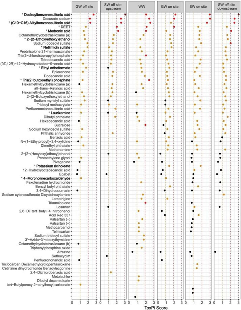
ToxPi scores calculated across sampling events for tentatively identified chemical features within site types (score <1: black; ≥1: orange; ≥2: red; ≥3:dark red). Chemical features are listed in order from largest summed ToxPi scores (top) to lowest (bottom). *Features making up ≥1% of total abundance in one or more sampling events, also indicated by bold text. Note: there was only one hit in the CompTox Dashboard for the following chemical formulae, therefore two features were tentatively identified as: hexamethylcyclotrisiloxane, labeled (a) and (b); and octamethylcyclotetrasiloxane, labeled (a) and (b). Valsartan was detected in both ESI-positive and ESI-negative modes in the same samples, labeled (+) and (−), respectively.

Searches of the reported chemical uses for tentatively identified features contributing to ≥1% total abundance and for which ToxPi scores could be calculated (i.e. those listed in Fig. 5) indicate that they generally consist of industrial use chemicals, surfactants, plasticizers, pharmaceuticals, personal care products, pesticides, and flame retardants, all of which were tentatively identified in wastewater, groundwater, and surface water samples (Table B.1). These use categories are similar to results obtained by an initial suspect screening analysis at the Jacksonville LTS (McEachran et al., 2018). A majority of the features also fell into more than one “use” and “functional use” category as listed in CPCat and CPDat databases, respectively (Table B.1). Other studies utilizing suspect screening approaches for the analysis of wastewater have detected industrial use chemicals, UV filters, and herbicides (Hug et al., 2014); pharmaceuticals and their active ingredients (Gago-Ferrero et al., 2015; Hug et al., 2014; Singer et al., 2016); as well as transformation products formed during wastewater treatment (Hug et al., 2014; Nürenberg et al., 2015; Schollée et al., 2016). Soulier et al. (2016) positively identified industrial use chemicals, pharmaceuticals, personal care products, and pesticides in a suspect screening analysis of groundwater, with pharmaceuticals making up the largest proportion detected. Industrial use chemicals, pharmaceuticals, and plant protection products were also detected and confirmed in ground- and surface waters via suspect screening in another study (Sjerps et al., 2016).

Chemicals including DEET, atrazine (herbicide), cetirizine dihydrochloride (antihistamine drug), losartan (antihypertensive drug), valsartan (antihypertensive drug), and triclocarban (antibacterial agent) which were tentatively identified here (Fig. 4; Fig. 5) have been detected in other studies (McEachran et al., 2018; Pochodylo and Helbling, 2017). The polyfluoroinated compounds perfluorononanoic acid (PFNA), 9-H-perfluorononanoic acid, 11-H-perfluoroundecanoic acid, perfluorooctanesulfonic acid (PFOS), perfluorohexane sulfonic acid (PFHxS) were also tentatively identified in this study (Fig. 4; Fig. 5); this group of chemicals is commonly found in environmental matrices and has been shown to have toxic effects on biota (e.g. reviewed by Ahrens, 2011; Buck et al., 2011). Interestingly, three of the micropollutants that were detected and reported by Pochodylo and Helbling (2017) as being rarely/never reported as contaminants in water were also tentatively identified in this study: levetiracetam (anticonvulsant drug; Fig. 4), fexofenadine hydrochloride (antihistamine drug; Fig. 5), and methocarbamol (muscle relaxant drug; Fig. 5).

Considering the lack of MS/MS data and confirmation using reference standards in this study, the results of prioritization for tentatively identified features is a tentative list only (i.e. those listed in Fig. 4 & Fig. 5). This priority list will be used for future targeted analyses of chemicals at the Jacksonville LTS in order to confirm their presence and for quantification. Results of this suspect screening analysis with subsequent confirmation of chemical features will provide researchers and water managers with information on COCs detected not only at this specific forested land application system, but can also be used to confirm whether these features are commonly found in other forested land application systems as a result of wastewater input.

4. Conclusion

This study represents the first comprehensive, watershed-scale study of COCs in a forested land application/water reuse site using a suspect screening approach to assess chemicals in wastewater effluent and ground- and surface waters. Wastewater typically contributed more chemical features to the chemical exposome of groundwater and surface water on site than from off-site waters. The input and subsequent fates of chemicals in receiving ground- and surface waters appear to be impacted by both precipitation and irrigation at the site, with soil drainage playing a key role. When comparing wastewater to ground- and surface waters on site, feature overlap increased during the sampling event which received the largest amount of irrigation. Further, this period also resulted in an increase of peak area abundances of features in on-site waters, though raw numbers of features detected were similar on and off site. This was counter to our initial expectation that wastewater would contribute to on-site waters the most during the period with the lowest amount of precipitation. Overall, numbers of chemical features detected and abundances across site types indicate impacts in receiving ground- and surface waters on site with dissipation and limited export of chemical features derived from wastewater in downstream surface waters. Prioritization of the chemical features tentatively identified in this study will allow for further examination of those which largely contribute to overall abundance as well as to potential human and environmental toxicity; the use of matched reference standards and additional targeted analyses will allow for confirmation of tentative identities of prioritized features and the quantification of those specific COCs in environmental samples. Considering that many of the tentatively identified COCs in this study have been detected in other wastewater effluents and environmental samples, we expect that many of these may likely be present in other, similar forest-water reuse systems, warranting further study on the potential for resulting impacts of these on humans and the environment.

References

- Ahrens L, 2011. Polyfluoroalkyl compounds in the aquatic environment: a review of their occurrence and fate. J. Environ. Monit 13, 20–31. 10.1039/c0em00373e. [DOI] [PubMed] [Google Scholar]
- Arias-Estévez M, López-Periago E, Martínez-Carballo E, Simal-Gándara J, Mejuto JC, García-Río L, 2008. The mobility and degradation of pesticides in soils and the pollution of groundwater resources. Agric. Ecosyst. Environ 123, 247–260. 10.1016/j.agee.2007.07.011. [DOI] [Google Scholar]
- Bastian RK, 2005. Interpreting science in the real world for sustainable land application. J. Environ. Qual 34, 174–183. [PubMed] [Google Scholar]
- Benotti MJ, Trenholm RA, Vanderford BJ, Holady JC, Stanford BD, Snyder SA, 2009. Pharmaceuticals and endocrine disrupting compounds in U.S. drinking water. Environ. Sci. Technol 43, 597–603. 10.1021/es801845a. [DOI] [PubMed] [Google Scholar]
- Benson R, Conerly OD, Sander W, Batt AL, Boone JS, Furlong ET, Glassmeyer ST, Kolpin DW,Mash HE, Schenck KM, Simmons JE, 2017. Human health screening and public health significance of contaminants of emerging concern detected in public water supplies. Sci. Total Environ 579, 1643–1648. 10.1016/j.scitotenv.2016.03.146. [DOI] [PMC free article] [PubMed] [Google Scholar]
- Birch AL, Emanuel RE, James AL, Nichols EG, 2016. Hydrologic impacts of municipal wastewater irrigation to a temperate forest watershed. J. Environ. Qual 45, 1303–1312. 10.2134/jeq2015.11.0577. [DOI] [PubMed] [Google Scholar]
- Bonferroni C, 1936. Teoria statistica delle classi e calcolo delle probabilit à. Pubbl. del R Ist. Super. di Sci. Econ. e Commer. di Firenze 8, 3–62. [Google Scholar]
- Buck RC, Franklin J, Berger U, Conder JM, Cousins IT, Voogt P.De, Jensen AA, Kannan K, Mabury SA, van Leeuwen SPJ, 2011. Perfluoroalkyl and polyfluoroalkyl substances in the environment: terminology, classification, and origins. Integr. Environ. Assess. Manag 7, 513–541. 10.1002/ieam.258. [DOI] [PMC free article] [PubMed] [Google Scholar]
- Buerge IJ, Poiger T, Müller MD, Buser H-R, 2003. Caffeine, an anthropogenic marker for wastewater contamination of surface waters. Environ. Sci. Technol 37, 691–700. 10.1021/es020125z. [DOI] [PubMed] [Google Scholar]
- Cahill JD, Furlong ET, Burkhardt MR, Kolpin D, Anderson LG, 2004. Determination of pharmaceutical compounds in surface- and ground-water samples by solidphase extraction and high-performance liquid chromatography-electrospray ionization mass spectrometry. J. Chromatogr. A 1041, 171–180. 10.1016/j.chroma.2004.04.005. [DOI] [PubMed] [Google Scholar]
- Cheng T, Zhao Y, Li X, Lin F, Xu Y, Zhang X, Li Y,Wang R, Lai L, 2007. Computation of octanol - water partition coefficients by guiding an additive model with knowledge. J. Chem. Inf. Model 47, 2140–2148. 10.1021/ci700257y. [DOI] [PubMed] [Google Scholar]
- Cincinelli A, Martellini T, Misuri L, Lanciotti E, Sweetman A, Laschi S, Palchetti I, 2012. PBDEs in Italian sewage sludge and environmental risk of using sewage sludge for land application. Environ. Pollut 161, 229–234. 10.1016/j.envpol.2011.11.001. [DOI] [PubMed] [Google Scholar]
- Clarke BO, Smith SR, 2011. Review of “emerging” organic contaminants in biosolids and assessment of international research priorities for the agricultural use of biosolids. Environ. Int 37, 226–247. 10.1016/j.envint.2010.06.004. [DOI] [PubMed] [Google Scholar]
- Crites RW, 1984. Land use of wastewater and sludge. Environ. Sci. Technol 18, 140A–147A. 10.1021/es00123a712. [DOI] [Google Scholar]
- Crohn DM, 1995. Sustainability of sewage sludge land application to northern hardwood forests. Ecol. Appl 5, 53–62. [Google Scholar]
- Diamond JM, Latimer HA, Munkittrick KR, Thornton KW, Bartell SM, Kidd KA, 2011. Prioritizing contaminants of emerging concern for ecological screening assessments. Environ. Toxicol. Chem 30, 2385–2394. 10.1002/etc.667. [DOI] [PubMed] [Google Scholar]
- Dionisio KL, Frame AM, Goldsmith MR, Wambaugh JF, Liddell A, Cathey T, Smith D, Vail J, Ernstoff AS, Fantke P, Jolliet O, Judson RS, 2015. Exploring consumer exposure pathways and patterns of use for chemicals in the environment. Toxicol. Reports 2, 228–237. 10.1016/j.toxrep.2014.12.009. [DOI] [PMC free article] [PubMed] [Google Scholar]
- Dionisio KL, Phillips K, Price PS, Grulke CM, Williams A, Biryol D, Hong T, Isaacs KK, 2018. Data descriptor: the chemical and products database, a resource for exposure-relevant data on chemicals in consumer products. Sci. Data 5, 180125. 10.1038/sdata.2018.125. [DOI] [PMC free article] [PubMed] [Google Scholar]
- Gago-Ferrero P, Schymanski EL, Bletsou AA, Aalizadeh R, Hollender J, Thomaidis NS, 2015. Extended suspect and non-target strategies to characterize emerging polar organic contaminants in raw wastewater with LC-HRMS/MS. Environ. Sci. Technol 49, 12333–12341. 10.1021/acs.est.5b03454. [DOI] [PubMed] [Google Scholar]
- Gosetti F, Mazzucco E, Gennaro MC, Marengo E, 2016. Contaminants in water: nontarget UHPLC/MS analysis. Environ. Chem. Lett 14, 51–65. 10.1007/s10311-015-0527-1. [DOI] [Google Scholar]
- Gushit JS, Ekanem EO, Adamu HM, Chindo IY, 2013. Analysis of herbicide residues and organic priority pollutants in selected root and leafy vegetable crops in plateau state, Nigeria. World J. Anal. Chem 1, 23–28. 10.12691/wjac-1-2-2. [DOI] [Google Scholar]
- Harrison EZ, Oakes SR, Hysell M, Hay A, 2006. Organic chemicals in sewage sludges. Sci. Total Environ 367, 481–497. 10.1016/j.scitotenv.2006.04.002. [DOI] [PubMed] [Google Scholar]
- Hedgespeth ML, Sapozhnikova Y, Pennington P, Clum A, Fairey A, Wirth E, 2012. Pharmaceuticals and personal care products (PPCPs) in treated wastewater discharges into Charleston Harbor, South Carolina. Sci. Total Environ 437, 1–9. 10.1016/j.scitotenv.2012.07.076. [DOI] [PubMed] [Google Scholar]
- Hollender J, Schymanski EL, Singer H, Ferguson PL, 2017. Non-target screening with high resolution mass spectrometry in the environment: ready to go? Environ. Sci. Technol 51, 11505–11512. 10.1021/acs.est.7b02184. [DOI] [PubMed] [Google Scholar]
- Hug C, Ulrich N, Schulze T, Brack W, Krauss M, 2014. Identification of novel micropollutants in wastewater by a combination of suspect and nontarget screening. Environ. Pollut 184, 25–32. 10.1016/j.envpol.2013.07.048. [DOI] [PubMed] [Google Scholar]
- Janda J, Nödler K, Brauch HJ, Zwiener C, Lange FT, 2018. Robust trace analysis of polar (C2-C8) perfluorinated carboxylic acids by liquid chromatography-tandem mass spectrometry: method development and application to surface water, groundwater and drinking water. Environ. Sci. Pollut. Res 26, 7326–7336. 10.1007/s11356-018-1731-x. [DOI] [PubMed] [Google Scholar]
- Karnjanapiboonwong A, Suski JG, Shah AA, Cai Q, Morse AN, Anderson TA, 2011. Occurrence of PPCPs at a wastewater treatment plant and in soil and groundwater at a land application site. Water Air Soil Pollut. 216, 257–273. 10.1007/s11270-010-0532-8. [DOI] [Google Scholar]
- Kaufman MM, Rogers DT,Murray KS, 2009. Using soil and contaminant properties to assess the potential for groundwater contamination to the lower Great Lakes, USA. Environ. Geol 56, 1009–1021. 10.1007/s00254-008-1202-7. [DOI] [Google Scholar]
- Kibuye FA, Gall HE, Elkin KR, Ayers B, Veith TL, Miller M, Jacob S, Hayden KR, Watson JE, Elliott HA, 2019. Fate of pharmaceuticals in a spray-irrigation system:from wastewater to groundwater. Sci. Total Environ 654, 197–208. 10.1016/j.scitotenv.2018.10.442. [DOI] [PubMed] [Google Scholar]
- Kipopoulou AM, Manoli E, Samara C, 1999. Bioconcentration of polycyclic aromatic hydrocarbons in vegetables grown in an industrial area. Environ. Pollut 106, 369–380. 10.1016/S0269-7491(99)00107-4. [DOI] [PubMed] [Google Scholar]
- Köck-schulmeyer M, Villagrasa M, López de Alda M, Céspedes-Sánchez R, Ventura F, Barceló D, 2013. Occurrence and behavior of pesticides in wastewater treatment plants and their environmental impact. Sci. Total Environ, 466–476 10.1016/j.scitotenv.2013.04.010. [DOI] [PubMed] [Google Scholar]
- Kruve A, 2018. Semi-quantitative non-target analysis of water with liquid chromatography/high-resolution mass spectrometry: how far are we? Rapid Commun. Mass Spectrom, 1–10 10.1002/rcm.8208. [DOI] [PubMed] [Google Scholar]
- Lampard J, Leusch F, Roiko A, Chapman H, 2010. Contaminants of concern in recycled water. Water 37, 54–60. [Google Scholar]
- Lesser LE, Mora A, Moreau C, Mahlknecht J, Hernández-Antonio A, Ramírez AI, Barrios-Piña H, 2018. Survey of 218 organic contaminants in groundwater derived from the world’s largest untreated wastewater irrigation system: Mezquital Valley, Mexico. Chemosphere 198, 510–521. 10.1016/j.chemosphere.2018.01.154. [DOI] [PubMed] [Google Scholar]
- Magesan GN, Wang H, 2003. Application of municipal and industrial residuals in New Zealand forests: an overview. Aust. J. Soil Res 41, 557–569. 10.1071/SR02134. [DOI] [Google Scholar]
- McEachran AD, Shea D, Bodnar W, Nichols EG, 2016. Pharmaceutical occurrence in groundwater and surface waters in forests land-applied with municipal wastewater. Environ. Toxicol. Chem 35, 898–905. 10.1002/etc.3216. [DOI] [PMC free article] [PubMed] [Google Scholar]
- McEachran AD, Shea D, Nichols EG, 2017a. Pharmaceuticals in a temperate forestwater reuse system. Sci. Total Environ 581–582, 705–714. 10.1016/j.scitotenv.2016.12.185. [DOI] [PMC free article] [PubMed] [Google Scholar]
- McEachran AD, Sobus JR,Williams AJ, 2017b. Identifying known unknowns using the US EPA’s CompTox Chemistry Dashboard. Anal. Bioanal. Chem 409, 1729–1735. 10.1007/s00216-016-0139-z. [DOI] [PubMed] [Google Scholar]
- McEachran AD, Hedgespeth ML, Newton SR, McMahen R, Strynar M, Shea D, Nichols EG, 2018. Comparison of emerging contaminants in receiving waters downstream of a conventional wastewater treatment plant and a forest-water reuse system. Environ. Sci. Pollut. Res 25, 12451–12463. 10.1007/s11356-018-1505-5. [DOI] [PMC free article] [PubMed] [Google Scholar]
- Merel S, Nikiforov AI, Snyder SA, 2015. Potential analytical interferences and seasonal variability in diethyltoluamide environmental monitoring programs. Chemosphere 127, 238–245. 10.1016/j.chemosphere.2015.02.025. [DOI] [PubMed] [Google Scholar]
- Morais SA, Delerue-Matos C, Gabarrell X, Blánquez P, 2013.Multimedia fatemodeling and comparative impact on freshwater ecosystems of pharmaceuticals from biosolids-amended soils. Chemosphere 93, 252–262. 10.1016/j.chemosphere.2013.04.074. [DOI] [PubMed] [Google Scholar]
- Newton SR, McMahen RL, Sobus JR, Mansouri K, Williams AJ, McEachran AD, Strynar MJ, 2018. Suspect screening and non-targeted analysis of drinking water using point-of-use filters. Environ. Pollut 234, 297–306. 10.1016/j.envpol.2017.11.033. [DOI] [PMC free article] [PubMed] [Google Scholar]
- Nichols EG, 2016. Current and future opportunities for forest land application systems of wastewater. In: Ansari AA, Gill SS, Gil R, Lanza GR, Newman L (Eds.), Phytoremediation - Management of Environmental Contaminants. vol. 4. Springer International Publishing, Switzerland, pp. 153–173. 10.1007/978-3-319-41811-7. [DOI] [Google Scholar]
- Nürenberg G, Schulz M, Kunkel U, Ternes TA, 2015. Development and validation of a generic nontarget method based on liquid chromatography - high resolution mass spectrometry analysis for the evaluation of different wastewater treatment options. J. Chromatogr. A 1426, 77–90. 10.1016/j.chroma.2015.11.014. [DOI] [PubMed] [Google Scholar]
- O’Connor GA, Elliott HA, Basta NT, Bastian RK, Pierzynski GM, Sims RC, Smith JE, 2004. Sustainable land application: an overview. J. Environ. Qual 34, 7–17. 10.1128/AEM.02358-12. [DOI] [PubMed] [Google Scholar]
- Pereira LC, de Souza AO, Bernardes MFF, Pazin M, Tasso MJ, Pereira PH, Dorta DJ, 2015. A perspective on the potential risks of emerging contaminants to human and environmental health. Environ. Sci. Pollut. Res 22, 13800–13823. 10.1007/s11356-015-4896-6. [DOI] [PubMed] [Google Scholar]
- Pochodylo AL, Helbling DE, 2017. Emerging investigators series: prioritization of suspect hits in a sensitive suspect screeningworkflowfor comprehensive micropollutant characterization in environmental samples. Environ. Sci. Water Res. Technol 3, 54–65. 10.1039/C6EW00248J. [DOI] [Google Scholar]
- R Core Team, 2013. R: A Language and Environment for Statistical Computing. [Google Scholar]
- Rager JE, Strynar MJ, Liang S, McMahen RL, Richard AM, Grulke CM, Wambaugh JF, Isaacs KK, Judson R, Williams AJ, Sobus JR, 2016. Linking high resolution mass spectrometry data with exposure and toxicity forecasts to advance highthroughput environmental monitoring. Environ. Int 88, 269–280. 10.1016/j.envint.2015.12.008. [DOI] [PubMed] [Google Scholar]
- Riemenschneider C, Al-Raggad M, Moeder M, Seiwert B, Salameh E, Reemtsma T, 2016. Pharmaceuticals, their metabolites, and other polar pollutants in field-grown vegetables irrigated with treated municipal wastewater. J. Agric. Food Chem 64, 5784–5792. 10.1021/acs.jafc.6b01696. [DOI] [PubMed] [Google Scholar]
- Rodil R, Quintana JB, López-Mahía P, Muniategui-Lorenzo S, Prada-Rodríguez D, 2009. Multi-residue analytical method for the determination of emerging pollutants in water by solidphase extraction and liquid chromatography-tandem mass spectrometry. J. Chromatogr. A 1216, 2958–2969. 10.1016/j.chroma.2008.09.041. [DOI] [PubMed] [Google Scholar]
- Ruff M, Mueller MS, Loos M, Singer HP, 2015. Quantitative target and systematic non-target analysis of polar organic micro-pollutants along the river Rhine using high-resolution mass-spectrometry - identification of unknown sources and compounds. Water Res. 87, 145–154. 10.1016/j.watres.2015.09.017. [DOI] [PubMed] [Google Scholar]
- Scheurer M, Storck FR, Graf C, Brauch H-J, Ruck W, Lev O, Lange FT, 2011. Correlation of six anthropogenic markers in wastewater, surface water, bank filtrate, and soil aquifer treatment. J. Environ. Monit 13, 966–973. 10.1039/c0em00701c. [DOI] [PubMed] [Google Scholar]
- Scheurer M, Nödler K, Freeling F, Janda J, Happel O, Riegel M,Müller U, Storck FR, Fleig M, Lange FT, Brunsch A, Brauch H-J, 2017. Small, mobile, persistent: trifluoroacetate in the water cycle – overlooked sources, pathways, and consequences for drinking water supply. Water Res. 126, 460–471. 10.1016/j.watres.2017.09.045. [DOI] [PubMed] [Google Scholar]
- Schollée JE, Schymanski EL, Hollender J, 2016. Statistical approaches for LC-HRMS data to characterize, prioritize, and identify transformation products from water treatment processes. In: Drewes JE, Letzel T (Eds.), Assessing Transformation Products of Chemicals by Non-Target and Suspect Screening − Strategies and Workflows. vol. 1. American Chemical Society, Washington, DC, pp. 45–65. 10.1021/bk-2016-1241.ch004. [DOI] [Google Scholar]
- Schymanski EL, Williams AJ, 2017. Open science for identifying “known unknown” chemicals. Environ. Sci. Technol 51, 5357–5359. 10.1021/acs.est.7b01908. [DOI] [PMC free article] [PubMed] [Google Scholar]
- Schymanski EL, Jeon J, Gulde R, Fenner K, Ruff M, Singer HP, Hollender J, 2014. Identifying small molecules via high resolution mass spectrometry: communicating confidence. Environ. Sci. Technol 48, 2097–2098. 10.1021/es5002105. [DOI] [PubMed] [Google Scholar]
- Schymanski EL, Singer HP, Slobodnik J, Ipolyi IM, Oswald P, Krauss M, Schulze T, Haglund P, Letzel T, Grosse S, Thomaidis NS, Bletsou A, Zwiener C, Ibáñez M, Portolés T, De Boer R, Reid MJ, Onghena M, Kunkel U, Schulz W, Guillon A, Noyon N, Leroy G, Bados P, Bogialli S, Stipaničev D, Rostkowski P, Hollender J, 2015. Non-target screening with high-resolution mass spectrometry: critical review using a collaborative trial on water analysis. Anal. Bioanal. Chem 407, 6237–6255. 10.1007/s00216-015-8681-7. [DOI] [PubMed] [Google Scholar]
- Sedlak DL, Gray JL, Pinkston KE, 2008. Understanding microcontaminants in recycled water. Environ. Sci. Technol 34, 508A–515A. 10.1021/es003513e. [DOI] [PubMed] [Google Scholar]
- Singer HP, Wössner AE, McArdell CS, Fenner K, 2016. Rapid screening for exposure to “non-target” pharmaceuticals from wastewater effluents by combining HRMS based suspect screening and exposure modeling. Environ. Sci. Technol 50, 6698–6707. 10.1021/acs.est.5b03332. [DOI] [PubMed] [Google Scholar]
- Sjerps RMA, Vughs D, van Leerdam JA, ter Laak TL, van Wezel AP, 2016. Datadriven prioritization of chemicals for various water types using suspect screening LC-HRMS. Water Res. 93, 254–264. 10.1016/j.watres.2016.02.034. [DOI] [PubMed] [Google Scholar]
- Sobus JR, Wambaugh JF, Isaacs KK, Williams AJ, McEachran AD, Richard AM, Grulke CM, Ulrich EM, Rager JE, Strynar MJ, Newton SR, 2018. Integrating tools for non-targeted analysis research and chemical safety evaluations at the US EPA. J. Expo. Sci. Environ. Epidemiol 28, 411–426. 10.1038/s41370-017-0012-y. [DOI] [PMC free article] [PubMed] [Google Scholar]
- Solomon KR, Velders GJM, Wilson SR, Madronich S, Longstreth J, Aucamp PJ, Bornman JF, 2016. Sources, fates, toxicity, and risks of trifluoroacetic acid and its salts: relevance to substances regulated under the Montreal and Kyoto protocols. J. Toxicol. Environ. Heal. Part B 19, 289–304. 10.1080/10937404.2016.1175981. [DOI] [PubMed] [Google Scholar]
- Soulier C, Coureau C, Togola A, 2016. Environmental forensics in groundwater coupling passive sampling and high resolution mass spectrometry for screening. Sci. Total Environ 563–564, 845–854. 10.1016/j.scitotenv.2016.01.056. [DOI] [PubMed] [Google Scholar]
- Strynar M, Dagnino S, McMahen R, Liang S, Lindstrom A, Andersen E, McMillan L, Thurman M, Ferrer I, Ball C, 2015. Identification of novel perfluoroalkyl ether carboxylic acids (PFECAs) and sulfonic acids (PFESAs) in natural waters using accurate mass time-of-flight mass spectrometry (TOFMS). Environ. Sci. Technol 49, 11622–11630. 10.1021/acs.est.5b01215. [DOI] [PubMed] [Google Scholar]
- Ulrich EM, Sobus JR, Grulke CM, Richard AM, Newton SR, Strynar MJ, Mansouri K, Williams AJ, 2019. EPA’s non-targeted analysis collaborative trial (ENTACT): genesis, design, and initial findings. Anal. Bioanal. Chem 411, 853–866. 10.1007/s00216-018-1435-6. [DOI] [PMC free article] [PubMed] [Google Scholar]
- USGS, 2004. Cleaning of equipment for water sampling (Ver. 2.0). In: Wilde FD (Ed.), National Field Manual for the Collection of Water-Quality Data - Handbooks for Water-Resources Investigations. U.S. Geological Survey, pp. 1–73. [Google Scholar]
- Vanderford BJ, Pearson RA, Rexing DJ, Snyder SA, 2003. Analysis of endocrine disruptors, pharmaceuticals, and personal care products in water using liquid chromatography/tandem mass spectrometry. Anal. Chem 75, 6265–6274. 10.1021/ac034210g. [DOI] [PubMed] [Google Scholar]
- Wild CP, 2005. Complementing the genome with an “exposome”: the outstanding challenge of environmental exposure measurement in molecular epidemiology. Cancer Epidemiol. Biomark. Prev 14, 1847–1850. 10.1158/1055-9965.EPI-05-0456. [DOI] [PubMed] [Google Scholar]
- Wild CP, 2012. The exposome: from concept to utility. Int. J. Epidemiol 41, 24–32. 10.1093/ije/dyr236. [DOI] [PubMed] [Google Scholar]
- Williams AJ, Grulke CM, Edwards J, Mceachran AD, Mansouri K, Baker NC, Patlewicz G, Shah I,Wambaugh JF, Judson RS, Richard AM, 2017. The CompTox Chemistry Dashboard: a community data resource for environmental chemistry. J. Cheminform 9, 1–27. 10.1186/s13321-017-0247-6. [DOI] [PMC free article] [PubMed] [Google Scholar]
- Wu X, Dodgen LK, Conkle JL, Gan J, 2015. Plant uptake of pharmaceutical and personal care products from recycled water and biosolids: a review. Sci. Total Environ 536, 655–666. 10.1016/j.scitotenv.2015.07.129. [DOI] [PubMed] [Google Scholar]
Associated Data
This section collects any data citations, data availability statements, or supplementary materials included in this article.