Generalized two‐tailed hypothesis testing for quantiles applied to the psychosocial status during the COVID‐19 pandemic

Abstract

Nonparametric tests do not rely on data belonging to any particular parametric family of probability distributions, which makes them preferable in case of doubt about the underlying population. Although the two‐tailed sign test is likely the most common nonparametric test for location problems, practitioners face serious drawbacks, such as its lack of statistical power and its inapplicability when information regarding data and hypotheses is uncertain or imprecise. In this paper, we generalize the two‐tailed sign test by embedding fuzzy hypotheses caused by uncertainty/imprecision regarding linguistic statements on fractions of underlying quantiles. By achieving this objective, (1) crucial limitations of the common two‐tailed sign test are mitigated/overcome, (2) various further strengths are incorporated into the sign test (e.g., meeting the trade‐off between point‐ and interval‐valued hypotheses, facilitated formulation of fuzzy hypotheses, standardization of membership functions), and (3) shortcomings that often come along with fuzzy hypothesis testing are avoided (e.g., higher complexity, fuzzy test decision, possibilistic interpretation of test results). In addition, we conduct a comprehensive case study using a real data set on the psychosocial status during the COVID‐19 pandemic. The results of the case study clearly indicate that the generalized two‐tailed sign test is preferable to the two‐tailed sign test with point‐ or interval‐valued hypotheses.

1. INTRODUCTION

Nonparametric tests are techniques of statistical inference that do not require the underlying distribution to meet specific assumptions, which is why they are also referred to as distribution‐free tests. These tests serve as alternatives to parametric tests that can only be applied when the data comply with certain assumptions and criteria. For instance, the common parametric one‐/two‐sample $t$‐test and one‐/two‐way analysis of variance (ANOVA) can be substituted by the nonparametric sign test, Mann–Whitney $U$‐test, Kruskal–Wallis test, and Friedman test, when there is any doubt about the underlying distribution (see, e.g., Grzegorzewski ¹ ).

In this paper, we focus on the sign test due to its importance and intuitive way of application when testing for quantiles. Against this backdrop, we highlight some benefits of the classical sign test (see, e.g., Grzegorzewski and Spiewak ² and Chukhrova and Johannssen ³ ): First, the sign test is versatile in application because it just makes few general assumptions about the underlying distribution. Thus, there are no problems resulting from biased verification of specific assumptions as the sign test is distribution‐free. Second, it tests for robust measures of location, that is, for quantiles. Third, the sign test does not require a large sample size. Fourth, the sign test is also applicable to ordinal data and paired‐sample data such as pre‐ and post‐treatment observations.

However, these advantages are offset by a few disadvantages (see, e.g., Chukhrova and Johannssen ⁴ ). Besides the well‐known loss of a good performance for small significance levels in combination with very small sample sizes, recent literature especially criticizes its exclusive application to classical problems where data and hypotheses are crisp, and thus a considerable rigidity regarding real‐life scenarios characterized by imprecision or uncertainty. To mitigate and/or to overcome this drawback, some authors have implemented techniques of fuzzy statistics into the classical sign test by utilizing concepts of fuzzy set theory (see for basic concepts the appendix of this paper, and moreover, we refer the interested reader to standard text books like Buckley, ^5,6 Klir and Yuan, ⁷ Kruse and Meyer, ⁸ Ross, ⁹ and Zimmermann ¹⁰ ). Most of these approaches are introduced to deal appropriately with fuzziness (or its interval‐valued subtype) in data and/or hypotheses formulation (see, e.g., Shafiq et al. ¹¹ ). On the one hand, some authors have considered fuzzy or interval‐valued data caused by the imprecision of observations (see Grzegorzewski, ¹² , ¹³ Grzegorzewski and Spiewak, ² , ¹⁴ Hesamian and Taheri, ¹⁵ Hesamian and Chachi, ¹⁶ Kahraman et al., ¹⁷ Momeni and Sadeghpour‐Gildeh ¹⁸ ). On the other hand, a few authors consider the hypotheses as fuzzy or interval‐valued caused by fuzzy quantiles like the fuzzy median (see Grzegorzewski and Spiewak ² , ¹⁴ ) or by imprecision of linguistic statements on quantiles (see Hesamian and Chachi, ¹⁶ Hesamian and Taheri, ¹⁵ and Momeni and Sadeghpour‐Gildeh ¹⁸ ). Recently, Chukhrova and Johannssen ³ have introduced a sign test for quantiles with fuzzy categories and/or fuzzy hypotheses, where fuzziness is caused by imprecision of linguistic statements on fractions of underlying quantiles. In comparison with the above mentioned approaches, the latter approach is characterized by a high degree of

• practicability due to the facilitated formulation of fuzzy hypotheses regarding fractions instead of quantiles (e.g., $H_0$: The population proportion is about $x\%$), since the basis of the sign test is the exact binomial test;

• generality, that is, specification of crisp and fuzzy areas in hypothesis formulation, consideration of the indifference zone by its gradual fuzzification, and thus flexible implementation of point‐valued, interval‐valued or fuzzy hypotheses (see Chukhrova and Johannssen ¹⁹ );

• standardization of modeling of membership functions for popular quantiles (such as the median or quartiles) in automated procedures like knowledge extraction from Big Data;

• convenience regarding the final (crisp) test decision that is in line with the classical test decision where the null hypothesis is either rejected or not rejected, and the generalized p value allows a common probabilistic interpretation.

However, Chukhrova and Johannssen ³ only consider the one‐tailed case, which is appropriate for testing whether the population proportion deviates from a reference value in one direction (left or right), but not in both directions as the most popular case in practice, the two‐tailed one. Assumed that the direction of interest is unknown, the two‐tailed case is to prefer to its one‐tailed counterpart, as it is easy in application (albeit more complex in derivation) and thus indispensable for new knowledge extraction, especially for given uncertainty/imprecision regarding the quantile of interest.

It is also worth noting that the recent literature is solely focused on comparisons of newly developed, that is, interval‐valued or fuzzy, approaches with the respective classical, mostly point‐valued, approach. However, this is only one side of the coin and there is the lack of an overall comparison regarding all these three closely related approaches. While in the one‐tailed case of the sign test a common point‐valued formulation of the null hypothesis $H_0$ leads to the same test conclusion as the respective interval‐valued alternative, there is a discrepancy between both approaches in the two‐tailed case, and thus a trade‐off with respect to their advantages and disadvantages. In contrast, the fuzzy approach, as a generalization of point‐ and interval‐valued approaches, could balance a disparity regarding precise/imprecise linguistic statements in hypothesis formulation, information value about the underlying distribution and the magnitude of the decision measure (e.g., the p value). Consequently, there is the need for a comparative study on the two‐tailed sign test with point‐ or interval‐valued hypotheses and its generalized version with fuzzy hypotheses.

In this paper, we extend the methodology proposed by Chukhrova and Johannssen ³ , ¹⁹ for the two‐tailed case and develop the generalized two‐tailed sign test for quantiles with fuzzy hypotheses caused by uncertainty/imprecision regarding linguistic statements on fractions of underlying quantiles. In addition, we compare the two‐tailed sign test with point‐ or interval‐valued hypotheses to the generalized test and discuss the advantages/disadvantages of all three approaches regarding their complexity, versatility and practicability.

To emphasize the benefits of the proposed generalized two‐tailed sign test for quantiles in comparison with point‐ and interval‐valued approaches, we conduct a comprehensive case study using a real data set on the psychosocial status during the COVID‐19 pandemic. In particular, we perform the two‐tailed sign test with point‐valued, interval‐valued and fuzzy hypotheses, and compare the obtained results in terms of test performance and implications for psychosocial status during the COVID‐19 pandemic. Moreover, we supplement the results of the generalized two‐tailed sign test by considering the respective results obtained in the one‐tailed case.

The paper is organized as follows. Section 2 introduces the two‐tailed sign test with point‐ or interval‐valued hypotheses. In Section 3, the generalized two‐tailed sign test with fuzzy hypotheses is proposed. Section 4 presents an extensive case study based on a real data set with regard to the psychosocial status during the COVID‐19 pandemic. Finally, in Section 5 the paper concludes with an overview of study results.

2. TWO‐TAILED SIGN TEST WITH POINT‐ OR INTERVAL‐VALUED HYPOTHESES

To make statements about an unknown quantile $M$ with $M\in \mathbb{R}$ of an underlying population (with c.d.f. presumed as continuous and strictly increasing in vicinity of $M$), we apply a common step‐wise test procedure that consists of the following four steps:

• 1Hypotheses formulation.
• 2Determination of sample size $n$ and level of significance $\alpha$.
• 3Drawing a random sample and computation of test statistic.
• 4Decision making by means of the p value.

Thus, in the first step, we formulate two‐tailed preliminary hypotheses $H_0^{\prime }$ and $H_1^{\prime }$ over the real numbers as complementary statements on $M$, say the median, with a hypothesized value $M^{*}$:

$$H_0^{\prime }:M=M^{*} \text{vs }{H}_1^{\prime }:M\ne M^{*}$$ (1)

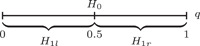
In Figure 1, $H_0^{\prime }$ and $H_1^{\prime }$ are illustrated graphically. The letters $l$ and $r$ in $H_{1l}^{\prime }$ and $H_{1r}^{\prime }$ point to the left and right position of the respective interval‐valued subset of $H_1^{\prime }$ in relation to the hypothesized value $M^{*}$. Since noncomplementary hypotheses have less relevance for a test of significance, we do not consider them in the following.

Figure 1.

Representation of preliminary hypotheses $H_0^{\prime }$, $H_1^{\prime }=H_{1l}^{\prime }\cup H_{1r}^{\prime }$

In addition, both hypotheses can be alternatively reformulated to complementary statements on the fraction $q$ of interest with parameter space $\mathrm{\Theta }≔\left(0,1\right)$ and a hypothesized fraction value, say 0.5 as in the case of the sign test on the median (see also Figure 2):

Figure 2.

Representation of reformulated hypotheses $H_0$, $H_1=H_{1l}\cup H_{1r}$

$$\begin{array}{ccc}\hfill & \hfill \hfill & H_0:\text{The population proportion}q\text{corresponds to}50\%\left(H_0:q=0.5\right)\hfill \\ \hfill & \hfill \hfill & H_1:\text{The population proportion}q\text{does not correspond to}50\%\left(H_1:q\ne 0.5\right)\hfill \end{array}$$ (2)

Consequently, the null hypothesis $H_0$ is simple and the alternative hypothesis $H_1$ is composite as in the case of preliminary hypotheses $H_0^{\prime }$ and $H_1^{\prime }$.

It should be noted that a simple null hypothesis allows the formulation of statements only regarding one quantile (here, the median). In contrast, a composite $H_0$ would provide the possibility to test on a set of quantiles simultaneously and thus lead to an additional gain of information regarding the population of interest. Moreover, an interval‐valued approach can map both situations with certainty in the formulation of the hypothesized quantile value, that is, as a crisp real number $M^{*}$, and also with some uncertainty/imprecision regarding linguistic statements on the fraction $q$ of the underlying quantile. For instance, given an uncertainty level of 20% regarding the 50%‐quantile, we can specify the hypotheses like

$$\begin{array}{ccc}\hfill & \hfill \hfill & H_0:\text{The population proportion}q\text{is between}40\%\text{and}60\%\left(H_0:0.4\le q\le 0.6\right)\hfill \\ \hfill & \hfill \hfill & H_1:\text{The population proportion}q\text{is not between}40\%\text{and}60\%\left(H_1:q<0.4,q>0.6\right)\hfill \end{array}$$

In the following, we propose to formulate interval‐ instead of point‐valued statements on $q$ using two hypothesized fraction values $q_{0l},q_{0r}$ and $q_{1l},q_{1r}$ for $H_0$ and $H_1$, respectively, that is,

$$H_0:q_{0l}\le q\le q_{0r} \text{vs }{H}_1:q\notin H_0\iff q<q_{1l},q>q_{1r} \text{with}{q}_{1l}=q_{0l}\le q_{0r}=q_{1r}$$ (3)

(see also Figure 3).

Figure 3.

Representation of reformulated interval‐valued hypotheses $H_0$, $H_1=H_{1l}\cup H_{1r}$

Following the classical test theory, we define subsets of the parameter space $\mathrm{\Theta }$ as crisp disjoint sets $H_0$, $H_1$, $I$ (i.e., it holds $H_0\cup H_1\cup I=\mathrm{\Theta }$) with indicator functions $m_{H_0}\left(q\right)$, $m_{H_1}\left(q\right)$, $m_I\left(q\right)$ (see Table 1, row 1–3). Here, the sets $H_0$, $H_1$, $I$ correspond to both hypotheses and the indifference zone. The sets $H_0$ and $H_1$ are nonempty, but the set $I$ is empty due to the complementary formulation of hypotheses. While the set $H_0$ is formulated as a real interval $\left[q_{0l},q_{0r}\right]$, the sets $H_1$ and $I$ are unions of two disjoint real intervals $H_{1l}$, $H_{1r}$ and $I_l$, $I_r$, respectively, which are located to the left (subscript $l$) or to the right (subscript $r$) of the set $H_0$. It is worth noting that an interval‐valued specification of $H_0$ simplifies to a point‐valued specification for $q_{0l}=q_{0r}$.

Table 1.

Subsets of the parameter space and their indicator functions

Set $H_0$	$\left\{q\in \mathrm{\Theta }|q_{0l}\le q\le q_{0r}\right\}$	$m_{H_0}\left(q\right)=\left\{\begin{array}{ccc}0\hfill & \text{if}\hfill & 0<q<q_{0l}\hfill \\ 1\hfill & \text{if}\hfill & q_{0l}\le q\le q_{0r}\hfill \\ 0\hfill & \text{if}\hfill & q_{0r}<q<1\hfill \end{array}\right.$
Set $H_1$	$H_{1l}\cup H_{1r}=\left\{q\in \mathrm{\Theta }|q<q_{1l},q>q_{1r}\right\}$	$m_{H_1}\left(q\right)=\left\{\begin{array}{ccc}1\hfill & \text{if}\hfill & 0<q<q_{1l}\hfill \\ 0\hfill & \text{if}\hfill & q_{1l}\le q\le q_{1r}\hfill \\ 1\hfill & \text{if}\hfill & q_{1r}<q<1\hfill \end{array}\right.$
Set $I$	$I_l\cup I_r=\left\{q\in \mathrm{\Theta }|q_{1l}\le q<q_{0l},q_{0r}<q\le q_{1r}\right\}$	$m_I\left(q\right)=\left\{\begin{array}{ccc}0\hfill & \text{if}\hfill & 0<q<q_{1l}\hfill \\ 1\hfill & \text{if}\hfill & q_{1l}\le q<q_{0l}\hfill \\ 0\hfill & \text{if}\hfill & q_{0l}\le q\le q_{0r}\hfill \\ 1\hfill & \text{if}\hfill & q_{0r}<q\le q_{1r}\hfill \\ 0\hfill & \text{if}\hfill & q_{1r}<q<1\hfill \end{array}\right.=0\forall q\in \mathrm{\Theta }$

According to the four‐step test procedure given above, in the second step, the sample size $n$, $n\in \mathbb{N}$, and the appropriate significance level $\alpha$, $\alpha \in \left(0,1\right)$, have to be specified. Although the determination of $n$ is up to the practitioner/researcher, it should not be set too small, otherwise problems arise due to increased probabilities of the type II error and situations where $H_0$ can hardly be rejected. For instance, at the 5% level of significance, $n\ge 6$ is necessary before any conclusion can be drawn (see Dixon and Mood ²⁰ ).

In the third step, a random sample of size $n$ is to draw from a continuous distribution, where the random variables $X_i$, $i=1,\text{…},n$, are stochastically independent and the quantile of interest $M$ is defined by the constraint $\mathbb{P}\left(X_i\le M\right)\in \left[q_{0l},q_{0r}\right]$. In addition, the continuous variable $X_i$ can be conveniently handled as categorical variable by means of a disjunctive coding 0/1 with respect to the category of interest: “negative signs” ($C^{(-)}$) or “positive signs” ($C^{(+)}$). Using indicator function $m_{C^{(-)}}\left(X_i\right)\in \left\{0,1\right\}$ or $m_{C^{(+)}}\left(X_i\right)\in \left\{0,1\right\}$, the test statistic can then be defined by the number of $X_i$ with $X_i<M^{*}$ or $X_i>M^{*}$, $i=1,\text{…},n$, depending on the specified success state $\mathbb{P}\left(m_{C^{(-)}}\left(X_i\right)=1\right)=q$ or $\mathbb{P}\left(m_{C^{(+)}}\left(X_i\right)=1\right)=1-q$. For instance, considering the membership of $X_i$ to $C^{(-)}$ as success, the test statistic $S={\sum }_{i=1}^n{m}_{C^{(-)}}\left(X_i\right)$ is binomial‐distributed with probability mass function

$$\mathbb{P}\left(S=s\right)=\left(\genfrac{}{}{0.0pt}{}{n}{s}\right)q^s{\left(1-q\right)}^{n-s}.$$

This also reveals that the sign test corresponds to an exact binomial test with power function $G_{n,c_l,c_r}\left(q\right)$, where $c_l$ and $c_r$ are the critical (rejection) values with $1\le c_l\le c_r\le n-1$, $c_l,c_r\in \mathbb{N}$. It also holds

$$G_{n,c_l,c_r}\left(q\right)=\underset{\text{first term}}{\underbrace{\sum _{m=0}^{c_l-1}\left(\genfrac{}{}{0.0pt}{}{n}{m}\right)q^m{\left(1-q\right)}^{n-m}}}+\underset{\text{second term}}{\underbrace{\sum _{m=c_r+1}^n\left(\genfrac{}{}{0.0pt}{}{n}{m}\right)q^m{\left(1-q\right)}^{n-m}}}=1-\sum _{m=c_l}^{c_r}\left(\genfrac{}{}{0.0pt}{}{n}{m}\right)q^m{\left(1-q\right)}^{n-m}$$ (4)

The power function determines probabilities for a correct rejection of $H_0$ ($q\in H_1$) and probabilities for a false rejection of $H_0$ ($q\in H_0$). It has as a rule an infimum for $q_m$, that is, $\underset{q\in \mathrm{\Theta }}{\text{inf}}{G}_{n,c_l,c_r}\left(q\right)=G_{n,c_l,c_r}\left(q_m\right)$, and is monotonically decreasing in the area to the left of $q_m$ and monotonically increasing in the area to the right of $q_m$. Due to the monotonicity of the power function in its respective domains $\left[0,q_m\right]$ and $\left[q_m,1\right]$, the argument value of the type I error criterion $E_1$, defined as the supremum of probabilities for false rejection of $H_0$, is one of the edge elements of the set $H_0$, that is,

$$E_1(n,c_l,c_r)=\underset{q\in H_0}{\text{sup}}{G}_{n,c_l,c_r}\left(q\right)=\max \left\{G_{n,c_l,c_r}\left(q_{0l}\right),G_{n,c_l,c_r}\left(q_{0r}\right)\right\}\le \alpha$$

Considering the symmetry of the power function in the case of a symmetrical specification of $q_{0l}$ and $q_{0r}$ regarding the 50%‐point, we obtain

$$E_1\left(n,c_l,c_r\right)=G_{n,c_l,c_r}\left(q_{0l}\right)=G_{n,c_l,c_r}\left(q_{0r}\right)\le \alpha$$

as well as

$$E_1(n,c_l,c_r)=G_{n,c_l,c_r}\left(0.5\right)=2\cdot 0.5^n\sum _{m=0}^{c_l-1}\left(\genfrac{}{}{0.0pt}{}{n}{m}\right)=0.5^{n-1}\sum _{m=0}^{c_l-1}\left(\genfrac{}{}{0.0pt}{}{n}{m}\right)\le \alpha$$

when $q_{0l}=q_{0r}=0.5$ holds (exemplary for a point‐valued formulation of $H_0$).

Finally, in the fourth step, the p value of the two‐tailed event is to compare with the predetermined $\alpha$‐level for making a test decision. Applying the general definition of the p value to the binomial test, we obtain

$$p_l(n,s)=\underset{q\in H_0}{\text{sup}}\mathrm{\mathbb{P}}(S\le s)=\max \left\{,\begin{array}{c}{\mathrm{\mathbb{P}}}_{q=q_{0l}}(S\le s)\\ {\mathrm{\mathbb{P}}}_{q=q_{0r}}(S\le s)\end{array}\right.=\max \left\{\begin{array}{c}\sum _{m=0}^s\left(\genfrac{}{}{0.0pt}{}{n}{m}\right)q_{0l}^m{(1-q_{0l})}^{n-m}\\ \sum _{m=0}^s\left(\genfrac{}{}{0.0pt}{}{n}{m}\right)q_{0r}^m{(1-q_{0r})}^{n-m}\end{array}\right.$$ (5)

and

$$p_r(n,s)=\underset{q\in H_0}{\text{sup}}\mathrm{\mathbb{P}}(S\ge s)=\max \left\{,\begin{array}{c}{\mathrm{\mathbb{P}}}_{q=q_{0l}}(S\ge s)\\ {\mathrm{\mathbb{P}}}_{q=q_{0r}}(S\ge s)\end{array}\right.=\max \left\{\begin{array}{c}\sum _{m=s}^n\left(\genfrac{}{}{0.0pt}{}{n}{m}\right)q_{0l}^m{(1-q_{0l})}^{n-m}\\ \sum _{m=s}^n\left(\genfrac{}{}{0.0pt}{}{n}{m}\right)q_{0r}^m{(1-q_{0r})}^{n-m}\end{array}\right.$$ (6)

for left‐ and right‐tailed events, respectively, and

$$p_c\left(n,s\right)=2\min \{p_l\left(n,s\right),p_r\left(n,s\right),0.5\}$$ (7)

for a two‐tailed event. Considering the case of $q_{0l}=q_{0r}=0.5$ (point‐valued $H_0$), the above definition of the “one‐tailed” p values reduces to

$$p_l\left(n,s\right)={\mathbb{P}}_{q=0.5}\left(S\le s\right)=0.5^n\sum _{m=0}^s\left(\genfrac{}{}{0.0pt}{}{n}{m}\right)\text{and}{p}_r\left(n,s\right)={\mathbb{P}}_{q=0.5}\left(S\ge s\right)=0.5^n\sum _{m=s}^n\left(\genfrac{}{}{0.0pt}{}{n}{m}\right)$$ (8)

The null hypothesis is to reject, if the p value for the two‐tailed event is lower than or equal to the given $\alpha$‐level, otherwise $H_0$ can not be rejected.

3. GENERALIZED TWO‐TAILED SIGN TEST WITH FUZZY HYPOTHESES

As well known, due to the monotonicity of the power function of the two‐tailed sign test in the area of $H_0$, the type I error generally increases and thus also the p value, by changing from point‐valued to interval‐valued statements in $H_0$. Further, this increase is the higher, the larger the width ($w=q_{1r}-q_{1l}$) of interval‐valued $H_0$, caused exemplary by the higher uncertainty/imprecision regarding the 50%‐quantile. To overcome these difficulties, a more promising way of modeling uncertainty/imprecision should be chosen via using fuzzy sets theory, that is, formulation of $H_0$ and $H_1$ via fuzzy sets instead of crisp sets as well as modeling of membership functions $m_{H_0}\left(q\right)$, $m_{H_1}\left(q\right)$ instead of indicator functions.

The most important benefits of fuzzy formulations of hypotheses compared to the interval‐valued approach are as follows:

• a gradual (and thus a more appropriate) modeling of uncertainty/imprecision regarding $H_0$ and $H_1$

• in general a reduction of the generalized type I error and the generalized p value

• better test results for smaller sample sizes

In the following, we extend the previous two‐tailed test problem to the case of fuzzy hypotheses by utilizing the general approach of Chukhrova and Johannssen. ¹⁹ Due to the fact that a fuzzy hypothesis is a generalization of a crisp hypothesis, we derive a generalized two‐tailed sign test following the four‐step procedure introduced in Section 2.

Therefore, in the first step, we consider fuzzy reformulated hypotheses $H_0$ and $H_1$ by embedding fuzzy statements on the fraction $q$ of interest. For instance,

$H_0:$ The population proportion $q$ is about 50% and rather lies between 40% and 60%

$$\left((,H_0:q=0.5,0.4\boxed{\le }q\boxed{\le }0.6\right)$$

$H_1:$ The population proportion $q$ is not about 50% and rather does not lie between 40% and 60%

$$\left(\left(,H_1:q<0.4,q\boxed{<}0.5,q\boxed{>}0.5,q>0.6,\right)\right)$$

In contrast to crisp reformulated hypothesis $H_0$, fuzzy reformulated null hypothesis

$$H_0:q_{0l}\le q\le q_{0r},q_{1l}\boxed{\le }q\boxed{\le }{q}_{1r}$$ (9)

with $0<q_{1l}\le q_{0l}\le q_{0r}\le q_{1r}<1$ is proposed to be formulated using

• 1.all four hypothesized fraction values (e.g., here $q_{0l}=q_{0r}=0.5$, $q_{1l}=0.4$, $q_{1r}=0.6$),
• 2.fuzzy comparison operators like “fuzzy” lower/larger equal ($\boxed{\le },\boxed{\ge }$) besides crisp comparison operators like “crisp” lower/larger equal ($\le ,\ge$),
• 3.gradual fuzzification of the indifference zone around the point‐ (interval‐)valued threshold (e.g., $\left[q_{1l},q_{0l}\right)=\left[0.4,0.5\right)$ and $\left(q_{0r},q_{1r}\right]=\left(0.5,0.6\right]$, given 50%‐threshold).

In Remark 3.1, we comment on points 1–3 regarding the above modeling approach.

Remark 3.1

• 1.In compliance with the theory proposed in Section 2, we consider in turn an indifference zone $I$, which can now be formulated also as a nonempty set, that is, $\left[q_{1l},q_{0l}\right)\cup \left(q_{0r},q_{1r}\right]$ with $q_{0l}\ne q_{1l}$, $q_{0r}\ne q_{1r}$. This formulation is quite natural, especially for given symmetric uncertainty (e.g., $|q_{0l}-q_{1l}|=|q_{0r}-q_{1r}|=10\%$) regarding the 50%‐point. Furthermore, a symmetric modeling of $I$ allows for an appropriate representation of the given percentage of the uncertainty level in the support of $H_0$, for example, given an uncertainty level of 20% one would choose the width of $H_0$ (i.e., the length of the support of $H_0$) as $w=q_{1r}-q_{1l}=0.2$, thus it holds $q_{0l}=q_{0r}=0.5$, $q_{1l}=0.4$ and $q_{1r}=0.6$.
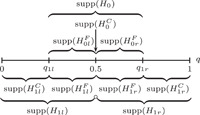
• 2.Due to the generalization of the crisp set $H_0$ to the fuzzy set $H_0$, the fuzzy set $H_0$ now consists of a crisp and a fuzzy set, that is, $H_0=H_0^C\cup H_0^F$, which are denoted as crisp and fuzzy areas of the null hypothesis. While crisp comparison operators refer to the crisp area of $H_0$, fuzzy comparison operators provide an indication of the fuzzy area of $H_0$ (see Figure 4). The edge elements of the nonempty supports of $H_{0l}^F$, $H_{0r}^F$ (with $H_{0l}^F\cup H_{0r}^F=H_0^F$) are thereby based on the hypothesized values $q_{1l}$, $q_{0l}$, $q_{0r}$, $q_{1r}$.
• 3.In contrast to the normal crisp area $H_0^C$, the fuzzy area $H_0^F\ne \varnothing$, whose support corresponds to the indifference zone, is subnormal. The membership functions $u_{0l}\left(q\right)$ and $u_{0r}\left(q\right)$ for this area are (strictly) monotonically increasing and decreasing functions.

Figure 4.

Representation of fuzzy reformulated hypotheses $H_0$, $H_1$

As for the formulation of fuzzy complementary hypothesis $H_1$ (see Figure 4), we propose to model this hypothesis in compliance with the definition of fuzzy $H_0$ in turn under full fuzzification of the indifference zone $\left[q_{1l},q_{0l}\right)\cup \left(q_{0r},q_{1r}\right]$ to the left and right of $H_0^C$, that is,

$$H_1:q<q_{1l},q\boxed{<}{q}_{0l},q\boxed{>}{q}_{0r},q>q_{1r}$$ (10)

where $H_1^C$ is the crisp area $\left(0,q_{1l}\right)\cup \left(q_{1r},1\right)$ and $H_1^F$ is the fuzzy area, whose support corresponds to the indifference zone.

In addition, we recapitulate the general formulation of both fuzzy hypotheses, that is, the definition of fuzzy sets $H_0$, $H_1$ and $I$ (with $H_0\cup H_1\cup I=\mathrm{\Theta }$), their crisp and fuzzy areas as well as of the corresponding membership functions $m_{H_0}\left(q\right)$, $m_{H_1}\left(q\right)$, $m_I\left(q\right)$ for $q\in \mathrm{\Theta }$ in Table 2.

Table 2.

Fuzzy subsets of the parameter space and their membership functions

Set $H_0$	$\begin{array}{c}\hfill \left\{\left(q;m_{H_0}\left(q\right)\right)|q\in \mathrm{\Theta },m_{H_0}\left(q\right)\in \left[0,1\right]\right\}\hfill \\ \text{ncl}\left(H_0\right)=\left\{q\in \mathrm{\Theta }|q_{0l}\le q\le q_{0r}\right\}\hfill \end{array}$	$m_{H_0}\left(q\right)=\left\{\begin{array}{ccc}0\hfill & \text{if}\hfill & 0<q<q_{1l}\hfill \\ m_{H_0^C}\left(q\right)\hfill & \text{if}\hfill & q=q_{1l}\hfill \\ u_{0l}\left(q\right)\hfill & \text{if}\hfill & q_{1l}<q<q_{0l}\hfill \\ 1\hfill & \text{if}\hfill & q_{0l}\le q\le q_{0r}\hfill \\ u_{0r}\left(q\right)\hfill & \text{if}\hfill & q_{0r}<q<q_{1r}\hfill \\ m_{H_0^C}\left(q\right)\hfill & \text{if}\hfill & q=q_{1r}\hfill \\ 0\hfill & \text{if}\hfill & q_{1r}<q<1\hfill \end{array}\right.$
Set $H_0^C$	$\begin{array}{c}\hfill \left\{\left(q;m_{H_0^C}\left(q\right)\right)|q\in \mathrm{\Theta },m_{H_0^C}\left(q\right)\in \left\{0,1\right\}\right\}\hfill \\ \text{supp}\left(H_0^C\right)=\left\{q\in \mathrm{\Theta }|q_{0l}\le q\le q_{0r}\right\}\hfill \end{array}$	$m_{H_0^C}\left(q\right)=\left\{\begin{array}{ccc}0\hfill & \text{if}\hfill & 0<q<q_{0l}\hfill \\ 1\hfill & \text{if}\hfill & q_{0l}\le q\le q_{0r}\hfill \\ 0\hfill & \text{if}\hfill & q_{0r}<q<1\hfill \end{array}\right.$
Set $H_0^F$	$\begin{array}{c}\left\{\left(q;m_{H_0^F}\left(q\right)\right)|q\in \mathrm{\Theta },m_{H_0^F}\left(q\right)\in \left[0,1\right]\right\}\hfill \\ \text{supp}\left(H_0^F\right)=\left\{q\in \mathrm{\Theta }|q_{1l}<q<q_{0l},q_{0r}<q<q_{1r}\right\}\hfill \end{array}$	$m_{H_0^F}\left(q\right)=\left\{\begin{array}{ccc}0\hfill & \text{if}\hfill & 0<q\le q_{1l}\hfill \\ u_{0l}\left(q\right)\hfill & \text{if}\hfill & q_{1l}<q<q_{0l}\hfill \\ 0\hfill & \text{if}\hfill & q_{0l}\le q\le q_{0r}\hfill \\ u_{0r}\left(q\right)\hfill & \text{if}\hfill & q_{0r}<q<q_{1r}\hfill \\ 0\hfill & \text{if}\hfill & q_{1r}\le q<1\hfill \end{array}\right.$
Set $H_1$	$\begin{array}{c}\left\{\left(q;m_{H_1}\left(q\right)\right)|q\in \mathrm{\Theta },m_{H_1}\left(q\right)\in \left[0,1\right]\right\}\hfill \\ \text{ncl}\left(H_1\right)=\left\{q\in \mathrm{\Theta }|q<q_{1l},q>q_{1r}\right\}\hfill \end{array}$	$m_{H_1}\left(q\right)=\left\{\begin{array}{ccc}1\hfill & \text{if}\hfill & 0<q<q_{1l}\hfill \\ u_{1l}\left(q\right)\hfill & \text{if}\hfill & q_{1l}\le q<q_{0l}\hfill \\ 0\hfill & \text{if}\hfill & q_{0l}\le q\le q_{0r}\hfill \\ u_{1r}\left(q\right)\hfill & \text{if}\hfill & q_{0r}<q\le q_{1r}\hfill \\ 1\hfill & \text{if}\hfill & q_{1r}<q<1\hfill \end{array}\right.$
Set $H_1^C$	$\begin{array}{c}\hfill \left\{\left(q;m_{H_1^C}\left(q\right)\right)|q\in \mathrm{\Theta },m_{H_1^C}\left(q\right)\in \left\{0,1\right\}\right\}\hfill \\ \text{supp}\left(H_1^C\right)=\left\{q\in \mathrm{\Theta }|q<q_{1l},q>q_{1r}\right\}\hfill \end{array}$	$m_{H_1^C}\left(q\right)=\left\{\begin{array}{ccc}1\hfill & \text{if}\hfill & 0<q<q_{1l}\hfill \\ 0\hfill & \text{if}\hfill & q_{1l}\le q\le q_{1r}\hfill \\ 1\hfill & \text{if}\hfill & q_{1r}<q<1\hfill \end{array}\right.$
Set $H_1^F$	$\begin{array}{c}\left\{\left(q;m_{H_1^F}\left(q\right)\right)|q\in \mathrm{\Theta },m_{H_1^F}\left(q\right)\in \left[0,1\right]\right\}\hfill \\ \text{supp}\left(H_1^F\right)=\left\{q\in \mathrm{\Theta }|q_{1l}\le q<q_{0l},q_{0r}<q\le q_{1r}\right\}\hfill \end{array}$	$m_{H_1^F}\left(q\right)=\left\{\begin{array}{ccc}0\hfill & \text{if}\hfill & 0<q<q_{1l}\hfill \\ u_{1l}\left(q\right)\hfill & \text{if}\hfill & q_{1l}\le q<q_{0l}\hfill \\ 0\hfill & \text{if}\hfill & q_{0l}\le q\le q_{0r}\hfill \\ u_{1r}\left(q\right)\hfill & \text{if}\hfill & q_{0r}<q\le q_{1r}\hfill \\ 0\hfill & \text{if}\hfill & q_{1r}<q<1\hfill \end{array}\right.$
Set $I$	$\left\{\left(q;m_I\left(q\right)\right)|q\in \mathrm{\Theta },m_I\left(q\right)\in \left\{0,1\right\}\right\}$	$m_I\left(q\right)=\left\{\begin{array}{ccc}0\hfill & \text{if}\hfill & 0<q<q_{1l}\hfill \\ 1\hfill & \text{if}\hfill & q_{1l}\le q<q_{0l}\hfill \\ 0\hfill & \text{if}\hfill & q_{0l}\le q\le q_{0r}\hfill \\ 1\hfill & \text{if}\hfill & q_{0r}<q\le q_{1r}\hfill \\ 0\hfill & \text{if}\hfill & q_{1r}<q<1\hfill \end{array}\right.$

Due to the fact that the fuzzy sets $H_0$ and $H_1$ are the unions of their crisp and fuzzy areas,

$$\begin{array}{ccc}\hfill & \hfill \hfill & \text{supp}\left(H_0\right)=\text{supp}\left(H_0^C\right)\cup \text{supp}\left(H_0^F\right),\hfill \\ \hfill & \hfill \hfill & \text{supp}\left(H_1\right)=\text{supp}\left(H_1^C\right)\cup \text{supp}\left(H_1^F\right),\hfill \end{array}$$

the membership functions $m_{H_0}\left(q\right)$ and $m_{H_1}\left(q\right)$ can be defined as follows:

$$\begin{array}{c}{m}_{H_0}\left(q\right)=m_{H_0^C\cup H_0^F}\left(q\right)=\max \left\{m_{H_0^C}\left(q\right),m_{H_0^F}\left(q\right)\right\}\\ m_{H_1}\left(q\right)=m_{H_1^C\cup H_1^F}\left(q\right)=\max \left\{m_{H_1^C}\left(q\right),m_{H_1^F}\left(q\right)\right\}\end{array}$$

Therefore, these complementary functions (i.e., $m_{H_0}\left(q\right)=1-m_{H_1}\left(q\right)$) are piecewise monotonically increasing and then monotonically decreasing (regarding $H_0$) or vice versa (regarding $H_1$). In the case of $q_{1l}=q_{0l}\le q_{0r}=q_{1r}$, hypotheses formulation reduces to crisp complementary hypotheses with $m_{H_0}\left(q\right)=m_{H_0}^C\left(q\right)$, $m_{H_1}\left(q\right)=m_{H_1}^C\left(q\right)$ (due to $H_0^F=\varnothing$, $H_1^F=\varnothing$).

As for the shape of the membership functions $m_{H_0}\left(q\right)$ and $m_{H_1}\left(q\right)$, we exemplary consider piecewise linear and $s$‐shaped functions with $u_{0l}\left(q\right)$, $u_{0r}\left(q\right)$ and $u_{1l}\left(q\right)$, $u_{1r}\left(q\right)$ given in Table 3. Figure 5 illustrates these membership functions and demonstrates the gradual fuzzification of the indifference zone $I$ (fuzzy complementary hypotheses). For a sensitivity analysis with regard to the impact of different shapes of membership functions (including piecewise linear and $s$‐shaped) in the framework of fuzzy hypothesis testing, we refer to Chukhrova and Johannssen. ²¹

Table 3.

Exemplary shapes of membership functions

Shape	Left‐tailed events	Right‐tailed events
linear	$u_{0l}\left(q\right)=\frac{q-q_{1l}}{q_{0l}-q_{1l}}\text{if}{q}_{1l}<q<q_{0l}$	$u_{0r}\left(q\right)=\frac{q_{1r}-q}{q_{1r}-q_{0r}}\text{if}{q}_{0r}<q<q_{1r}$
	$u_{1l}\left(q\right)=\frac{q_{0l}-q}{q_{0l}-q_{1l}}\text{if}{q}_{1l}\le q<q_{0l}$	$u_{1r}\left(q\right)=\frac{q-q_{0r}}{q_{1r}-q_{0r}}\text{if }{q}_{0r}<q\le q_{1r}$
$s$‐shaped (polynomial)	$u_{0l}\left(q\right)=\left\{\begin{array}{cc}2{\left(\frac{q-q_{1l}}{q_{0l}-q_{1l}}\right)}^2& \text{if }{q}_{1l}\le q<\frac{q_{0l}+q_{1l}}{2}\\ 1-2{\left(\frac{q_{0l}-q}{q_{0l}-q_{1l}}\right)}^2& \text{if }\frac{q_{0l}+q_{1l}}{2}\le q<q_{0l}\end{array}\right.$	$u_{0r}\left(q\right)=\left\{\begin{array}{cc}1-2{\left(\frac{q-q_{0r}}{q_{1r}-q_{0r}}\right)}^2& \text{if }{q}_{0r}<q\le \frac{q_{0r}+q_{1r}}{2}\\ 2{\left(\frac{q_{1r}-q}{q_{1r}-q_{0r}}\right)}^2& \text{if }\frac{q_{0r}+q_{1r}}{2}<q\le q_{1r}\end{array}\right.$
	$u_{1l}\left(q\right)=\left\{\begin{array}{cc}1-2{\left(\frac{q-q_{1l}}{q_{0l}-q_{1l}}\right)}^2& \text{if }{q}_{1l}\le q<\frac{q_{0l}+q_{1l}}{2}\\ 2{\left(\frac{q_{0l}-q}{q_{0l}-q_{1l}}\right)}^2& \text{if }\frac{q_{0l}+q_{1l}}{2}\le q<q_{0l}\end{array}\right.$	$u_{1r}\left(q\right)=\left\{\begin{array}{cc}2{\left(\frac{q-q_{0r}}{q_{1r}-q_{0r}}\right)}^2& \text{if }{q}_{0r}<q\le \frac{q_{0r}+q_{1r}}{2}\\ 1-2{\left(\frac{q_{1r}-q}{q_{1r}-q_{0r}}\right)}^2& \text{if }\frac{q_{0r}+q_{1r}}{2}<q\le q_{1r}\end{array}\right.$

Figure 5.

Fuzzy complementary piecewise linear and polynomial ($s$‐shaped) membership functions [Color figure can be viewed at wileyonlinelibrary.com]

In the second step, the practitioner/researcher determines the sample size $n$, $n\in \mathbb{N}$, and the magnitude of the $\alpha$‐level, $\alpha \in \left(0,1\right)$. In the third step, the test statistic can be calculated via ${\sum }_{i=1}^n{m}_{C^{(-)}}\left(X_i\right)$ by using observations obtained from a random sample. Finally, in the fourth step, the user compares the generalized p value for the two‐tailed event with the predetermined $\alpha$‐level to achieve a crisp test decision. Note that the criteria for decision making are the same as in the case of crisp hypothesis testing.

As for the calculation of the generalized p value, we can use the results obtained in Section 2 solely for the elements from the crisp area of $H_0$. Therefore, the definition of the p value is first to generalize with respect to the fuzzy area of $H_0$. In particular, this generalization shall be conducted in compliance with the definition of the generalized type I error criterion,

$$E_1(n,c_l,c_r)=\underset{q\in H_0}{\text{sup}}\left\{(m_{H_0}\left(q\right)-m_{H_1}\left(q\right))G_{n,c_l,c_r}\left(q\right)\right\}\le \alpha ,$$ (11)

which is given by the supremum of weighted probabilities for a false rejection of the null hypothesis (see Arnold ²² , ²³ ). While the probabilities originate from the power function $G_{n,c_l,c_r}\left(q\right)$, the weight function is defined by the difference between the membership of an element $q\in \mathrm{\Theta }$ to fuzzy $H_0$ and to fuzzy $H_1$, that is, it holds $m_{H_0}\left(q\right)-m_{H_1}\left(q\right)$ for all $q\in \mathrm{\Theta }$. Definition (11) can also be stated as

$$\begin{array}{lll}{E}_1(n,c_l,c_r)& =& \underset{q\in \text{supp}\left(H_0\right)}{\text{sup}}\left\{(m_{H_0}\left(q\right)-m_{H_1}\left(q\right))G_{n,c_l,c_r}\left(q\right)\right\}\\ & =& \max \left\{\begin{array}{c}\underset{q\in \text{supp}\left(H_0^C\right)}{\text{sup}}\left\{(m_{H_0}\left(q\right)-m_{H_1}\left(q\right))G_{n,c_l,c_r}\left(q\right)\right\}\\ \underset{q\in \text{supp}\left(H_0^F\right)}{\text{sup}}\left\{(m_{H_0}\left(q\right)-m_{H_1}\left(q\right))G_{n,c_l,c_r}\left(q\right)\right\}\end{array}\right\}\\ & =& \max \left\{\begin{array}{c}{G}_{n,c_l,c_r}\left(q_{0l}\right)\\ G_{n,c_l,c_r}\left(q_{0r}\right)\\ \underset{q\in \text{supp}\left(H_0^F\right)}{\text{sup}}\left\{(m_{H_0}\left(q\right)-m_{H_1}\left(q\right))G_{n,c_l,c_r}\left(q\right)\right\}\end{array}\right\}\end{array}$$

against the backdrop that the domain for the supremum of weighted probabilities can logically be restricted to elements of $H_0$ that involve positive weights of the power function. Further, in compliance with the classical sign test, the generalized type I error criterion $E_1$ has a supremum for the elements of the respective support of $H_0^C$ at $q=q_{0l}$ or $q=q_{0r}$, that is, $\max \left\{G_{n,c_l,c_r}\left(q_{0l}\right),G_{n,c_l,c_r}\left(q_{0r}\right)\right\}$, where $G_{n,c_l,c_r}\left(q_{0l}\right)=G_{n,c_l,c_r}\left(q_{0r}\right)$ holds for $q_{0l}=q_{0r}$. This is due to (1) the monotonically decreasing (increasing) power function $G_{n,c_l,c_r}\left(q\right)$ to the left (right) of its minimum,

$$\underset{q\in \mathrm{\Theta }}{\min }{G}_{n,c_l,c_r}\left(q\right)=G_{n,c_l,c_r}\left(q_m\right),$$ (12)

as well as to (2) the relationship $m_{H_0}\left(q\right)-m_{H_1}\left(q\right)=1\text{for all}q\in \text{supp}\left(H_0^C\right)$.

Besides the supremum with respect to $\text{supp}\left(H_0^C\right)$, $E_1$ has another supremum for $q\in \text{supp}\left(H_0^F\right)$ (given $\text{supp}\left(H_0^F\right)\ne \varnothing$). However, it is generally not representable in a closed form caused by the reverse monotonicity of both the power and weight functions, which is why it has to be calculated numerically, and after that, it is to compare with the supremum from the support of the crisp area. Note that we obtain crisp hypotheses and therefore the results presented in Section 2 when the support of the fuzzy area is an empty set.

Using the above results, we define the generalized p value for a left‐tailed, right‐tailed and two‐tailed event as follows:

$$p_l(n,s)=\underset{q\in H_0}{\text{sup}}\left\{(m_{H_0}\left(q\right)-m_{H_1}\left(q\right))\mathrm{\mathbb{P}}(S\le s)\right\}=\underset{q\in H_0}{\text{sup}}\left\{(m_{H_0}\left(q\right)-m_{H_1}\left(q\right))\sum _{m=0}^s\left(\genfrac{}{}{0.0pt}{}{n}{m}\right)q^m{(1-q)}^{n-m}\right\}$$ (13)

$$p_r\left(n,s\right)=\underset{q\in H_0}{\text{sup}}\left\{\left(m_{H_0}\left(q\right)-m_{H_1}\left(q\right)\right)\mathbb{P}\left(S\ge s\right)\right\}=\underset{q\in H_0}{\text{sup}}\left\{\left(m_{H_0}\left(q\right)-m_{H_1}\left(q\right)\right)\sum _{m=s}^n\left(\genfrac{}{}{0.0pt}{}{n}{m}\right)q^m{\left(1-q\right)}^{n-m}\right\}$$ (14)

$$p_g\left(n,s\right)=2\min \left\{\begin{array}{c}\hfill \underset{q\in H_0}{\text{sup}}\left\{\left(m_{H_0}\left(q\right)-m_{H_1}\left(q\right)\right)\mathbb{P}\left(S\le s\right)\right\}\hfill \\ \hfill \underset{q\in H_0}{\text{sup}}\left\{\left(m_{H_0}\left(q\right)-m_{H_1}\left(q\right)\right)\mathbb{P}\left(S\ge s\right)\right\}\hfill \\ \hfill 0.5\hfill \end{array}\right\}$$ (15)

where (15) corresponds to

$$\begin{array}{ccc}{p}_g(n,s)& =& 2\min \left\{\begin{array}{c}\max \left\{\begin{array}{c}{\text{sup}}_{q\in \text{supp}\left(H_0^C\right)}\left\{(m_{H_0}\left(q\right)-m_{H_1}\left(q\right))\mathrm{\mathbb{P}}(S\le s)\right\}\\ {\text{sup}}_{q\in \text{supp}\left(H_0^F\right)}\left\{(m_{H_0}\left(q\right)-m_{H_1}\left(q\right))\mathrm{\mathbb{P}}(S\le s)\right\}\end{array}\right\}\\ \max \left\{\begin{array}{c}{\text{sup}}_{q\in \text{supp}\left(H_0^C\right)}\left\{(m_{H_0}\left(q\right)-m_{H_1}\left(q\right))\mathrm{\mathbb{P}}(S\ge s)\right\}\\ {\text{sup}}_{q\in \text{supp}\left(H_0^F\right)}\left\{(m_{H_0}\left(q\right)-m_{H_1}\left(q\right))\mathrm{\mathbb{P}}(S\ge s)\right\}\end{array}\right\}\\ 0.5\end{array}\right\}\\ & =& 2\min \left\{\begin{array}{c}\max \left\{\begin{array}{c}\sum _{m=0}^s\left(\genfrac{}{}{0.0pt}{}{n}{m}\right)q_{0l}^m{(1-q_{0l})}^{n-m}\\ \sum _{m=0}^s\left(\genfrac{}{}{0.0pt}{}{n}{m}\right)q_{0r}^m{(1-q_{0r})}^{n-m}\\ {\text{sup}}_{q\in \text{supp}\left(H_0^F\right)}\left\{(m_{H_0}\left(q\right)-m_{H_1}\left(q\right))\mathrm{\mathbb{P}}(S\le s)\right\}\end{array}\right\}\\ \max \left\{\begin{array}{c}\sum _{m=s}^n\left(\genfrac{}{}{0.0pt}{}{n}{m}\right)q_{0l}^m{(1-q_{0l})}^{n-m}\\ \sum _{m=s}^n\left(\genfrac{}{}{0.0pt}{}{n}{m}\right)q_{0r}^m{(1-q_{0r})}^{n-m}\\ {\text{sup}}_{q\in \text{supp}\left(H_0^F\right)}\left\{(m_{H_0}\left(q\right)-m_{H_1}\left(q\right))\mathrm{\mathbb{P}}(S\ge s)\right\}\end{array}\right\}\\ 0.5\end{array}\right\}\end{array}$$

by an additional distinction between crisp and fuzzy areas. For $q_{0l}=q_{0r}$, the definition of the generalized p value simplifies to

$$\begin{array}{ccc}{p}_g(n,s)& =& 2\min \left\{\begin{array}{c}\max \left\{\begin{array}{c}\sum _{m=0}^s\left(\genfrac{}{}{0.0pt}{}{n}{m}\right)q_{0l}^m{(1-q_{0l})}^{n-m}\\ {\text{sup}}_{q\in \text{supp}\left(H_0^F\right)}\left\{(m_{H_0}\left(q\right)-m_{H_1}\left(q\right))\mathrm{\mathbb{P}}(S\le s)\right\}\end{array}\right\}\\ \max \left\{\begin{array}{c}\sum _{m=s}^n\left(\genfrac{}{}{0.0pt}{}{n}{m}\right)q_{0l}^m{(1-q_{0l})}^{n-m}\\ {\text{sup}}_{q\in \text{supp}\left(H_0^F\right)}\left\{(m_{H_0}\left(q\right)-m_{H_1}\left(q\right))\mathrm{\mathbb{P}}(S\ge s)\right\}\end{array}\right\}\\ 0.5\end{array}\right\}\\ & =& 2\min \left\{\begin{array}{c}\max \left\{\begin{array}{c}{\text{0.5}}^n\sum _{m=0}^s\left(\genfrac{}{}{0.0pt}{}{n}{m}\right)\\ {\text{sup}}_{q\in \text{supp}\left(H_0^F\right)}\left\{(m_{H_0}\left(q\right)-m_{H_1}\left(q\right))\mathrm{\mathbb{P}}(S\le s)\right\}\end{array}\right\}\\ \max \left\{\begin{array}{c}{\text{0.5}}^n\sum _{m=s}^n\left(\genfrac{}{}{0.0pt}{}{n}{m}\right)\\ {\text{sup}}_{q\in \text{supp}\left(H_0^F\right)}\left\{(m_{H_0}\left(q\right)-m_{H_1}\left(q\right))\mathrm{\mathbb{P}}(S\ge s)\right\}\end{array}\right\}\\ 0.5\end{array}\right\}\end{array}$$ (16)

where (16) holds when choosing $q_{0l}=q_{0r}=0.5$.

Considering exemplary the last case ($q_{0l}=q_{0r}=0.5$), we propose to interpret the combined test decision, that is, the generalized p value, in turn under separate consideration of crisp and fuzzy areas. In particular, the p value

$$p_c=2\min \left\{\begin{array}{c}0.5^n\sum _{m=0}^s\left(\genfrac{}{}{0.0pt}{}{n}{m}\right)\hfill \\ 0.5^n\sum _{m=s}^n\left(\genfrac{}{}{0.0pt}{}{n}{m}\right)\hfill \end{array}\right\}$$

related to the crisp area $H_0^C$ of fuzzy $H_0$ leads to a probabilistic p value, which corresponds to the p value of the common test on the median with point‐valued formulated $H_0$. In contrast, the weighted p value

$$p_f=2\min \left\{\begin{array}{c}{\text{sup}}_{q\in \text{supp}\left(H_0^F\right)}\left\{(m_{H_0}\left(q\right)-m_{H_1}\left(q\right))\mathrm{\mathbb{P}}(S\le s)\right\}\\ {\text{sup}}_{q\in \text{supp}\left(H_0^F\right)}\left\{(m_{H_0}\left(q\right)-m_{H_1}\left(q\right))\mathrm{\mathbb{P}}(S\ge s)\right\}\end{array}\right\}$$

related to the fuzzy area $H_0^F$ of fuzzy $H_0$ approximates the (maximum possible) probabilistic p value of the common test on quantiles with interval‐valued $H_0$ (formulated without median) by means of appropriate extent constituted by fuzziness (relaxation) of hypotheses formulation. Thus, the fuzzy test on quantiles is related to both tests (and their decisions) and combines them by means of the generalized p value $p_g$. As for the rejection of fuzzy $H_0$ (based on $p_g\le \alpha$) in favor of fuzzy $H_1$, we can generally accept fuzzy $H_1$ at the chosen level of significance $\alpha$ due to the significant result. Considering the nonrejection of fuzzy $H_0$ (based on $p_g>\alpha$), we fail to reject fuzzy $H_0$ at the chosen level of significance $\alpha$ due to the nonsignificant result. Such a crisp decision making corresponds to classical decision making either for point‐valued or interval‐valued $H_0$.

In addition, we refer to the possibility of obtaining final exploratory results (following a rejection of fuzzy $H_0$) by considering the magnitude of the realization of the test statistic $s$:

• There is a deviation of the true quantile $M$ to the left from the hypothesized quantile $M^{*}$, given $s>\frac{n}{2}$.

• There is a deviation of the true quantile $M$ to the right from the hypothesized quantile $M^{*}$, given $s<\frac{n}{2}$.

It is important to note that such findings are not referred to as test results in the sense of significant conclusions due to a possible type III error, which entails an incorrect decision of direction following a rejected null hypothesis of a two‐tailed test (see Kaiser ²⁴ ).

4. CASE STUDY: PSYCHOSOCIAL STATUS DURING THE COVID‐19 PANDEMIC

In this case study, we intend to investigate the psychosocial status during the COVID‐19 pandemic. For this purpose, we compare the results of the two‐tailed sign test with point‐valued, interval‐valued and fuzzy hypotheses. To complete the statistical analysis, we supplement the results of the generalized two‐tailed sign test by considering the respective results when implementing one‐tailed fuzzy hypotheses introduced by Chukhrova and Johannssen. ³

4.1. The data set

The data set, the COVIDiSTRESS global survey, underlying this case study is taken from Yamada et al. ²⁵ Following COVIDiSTRESS global survey network, ²⁶ this survey is an international collaborative undertaking for data gathering on human experiences, behavior, and attitudes during the COVID‐19 pandemic between March 30 and May 30, 2020. The survey focuses on investigation of eight variables (see Table 4) regarding psychological stress, compliance with behavioral guidelines to slow the spread of coronavirus type 2 as well as trust in governmental institutions and their preventive measures.

Table 4.

Variables of the COVIDiSTRESS global survey

Variable	Description	Measurement
PSS‐10	Perceived stress for the past week	PSS, 10 items, 5‐point Likert scale
SPS‐10	Available social provisions in critical/distressing situations	SPS, 10 items, 6‐point Likert scale
SLON‐3	Short self‐report scale of loneliness for the last week	SLON, 3 items, 5‐point Likert scale
BFI‐1	Big 5—Extraversion	BFI Short, 3 items, 6‐point Likert scale
BFI‐2	Big 5—Neuroticism	BFI Short, 3 items, 6‐point Likert scale
BFI‐3	Big 5—Openness to experience	BFI Short, 3 items, 6‐point Likert scale
BFI‐4	Big 5—Agreeableness	BFI Short, 3 items, 6‐point Likert scale
BFI‐5	Big 5—Conscientiousness	BFI Short, 3 items, 6‐point Likert scale

Abbreviations: BFI, Big Five Inventory; PSS, Perceived Stress Scale; SLON, Scale of LONeliness; SPS, Social Provisions Scale.

The variables given in Table 4 are explained in more detail in the following:

• PSS‐10 is an instrument for assessing perceived stress and includes two subscales: perceived helplessness (six items) and perceived self‐efficacy (four items). Psychological stress is associated with an increased risk of disease (see, e.g., Klein et al. ²⁷ and Bastianon et al. ²⁸ ).

• SPS‐10 is an instrument designed to measure the perceived availability of social support and includes five subscales with two items each: emotional support or bonding, social integration, affirmation of worth, material support, and orientation. Perception of social support is one of the best predictors of psychological distress and quality of life (see, e.g., Ibarra‐Rovillard & Kuiper, ²⁹ Caron, ³⁰ Iapichino et al., ³¹ Steigen & Bergh ³² ).

• SLON‐3 is an instrument designed to measure the subjective emotional experience of loneliness and includes three items. SLON‐3 is a subscale of the UCLA loneliness scale that contains 20 items (see, e.g., Hughes et al., ³³ ).

• BFI‐1–BFI‐5 are five subscales of the Big Five Inventory (see John ³⁴ ) with three items each. The Big Five approach is a psychological concept for assessing personality (see McCrae and John ³⁵ ). Central to this approach is the assumption that personality differences between individuals, expressed in behavioral and experiential terms, are due to the five central personality dimensions of Openness to experience, Conscientiousness, Extraversion, Agreeableness, and Neuroticism (this is why this approach is also called OCEAN model) (see, e.g., Lang et al. ³⁶ ).

It is worth noting that the higher the score on the respective Likert scale (see third column of Table 4), the higher the perceived stress (PSS‐10), the higher the perceived availability of social support (SPS‐10), the higher the subjective emotional experience of loneliness (SLON‐3) or the more distinct the respective psychosocial attribute (BFI‐1–BFI‐5). The respective scores were surveyed for 27 European countries and 15 countries from other continents (North America, South America, Asia, and Australia), the sample size per country varies between 216 (Ireland) and 22,933 (Finland). For each country and each variable, descriptive statistics, such as scale means, have been calculated, see tables 9–16 in Yamada et al. ²⁵

4.2. Design and objective of this case study

In this case study, we examine the psychosocial status during the corona pandemic in European countries measured by means of eight variables of the COVIDiSTRESS global survey. As the psychosocial status may be considerably different for various regions of Europe due to structural factors, cultural circumstances and climatic aspects, it is not appropriate to analyze all the European countries as a collective pool. For this reason, we divide the pool into three subgroups according to European regions: Western, Eastern, and Southern Europe (see Table 5). On the one hand, such a handling reduces the sample size, but on the other hand it allows much more target group‐specific conclusions.

Table 5.

European countries

	1	2	3	4	5	6	7	8	9	10	11
Western Europe (WE)	Austria	Belgium	Denmark	Finland	France	Germany	Ireland	Netherlands	Sweden	Switzerland	United Kingdom
Eastern Europe (EE)	Bulgaria	Croatia	Czech Republic	Hungary	Lithuania	Poland	Romania	Slovakia
Southern Europe (SE)	Bosnia and Herzegovina	Greece	Italy	Kosovo	Portugal	Serbia	Spain	Turkey

The scale means for the eight variables across the European countries are given in Table 6. Since significant upwards or downwards deviations from a benchmark value are associated with significantly stronger or weaker psychosocial effects, it is important to investigate whether there are significant deviations in both directions, that is, to employ a suitable two‐tailed test. Due to the division of the entire data set into three subgroups of interest, we are confronted with rather small sample sizes (8–11 observations per subgroup) and thus the nonparametric sign test is a reasonable choice to test for the median with respect to a single subgroup. As the underlying sample sizes for each country are very large ($n\ge 216$, on average $n=\mathrm{3,346}$, for each country), it is appropriate to assume a normal distribution for the observations of the individual countries. Due to the symmetry of the normal distribution, the mean corresponds to the median. Thus, we can use the respective scale means as observed values within the subgroup of interest for testing on the median. As for achieving a corresponding hypothesized median value $M^{*}$ with respect to the investigated variable, it is reasonable to take the class midpoint of the underlying Likert scale as a benchmark value (see also Table 6).

Table 6.

Mean values of investigated variables for European countries

	PSS‐10 ($M^{*}=3$)			SPS‐10 ($M^{*}=3.5$)			SLON‐3 ($M^{*}=3$)			BFI‐1 ($M^{*}=3.5$)			BFI‐2 ($M^{*}=3.5$)			BFI‐3 ($M^{*}=3.5$)			BFI‐4 ($M^{*}=3.5$)			BFI‐5 ($M^{*}=3.5$)
Country	WE	EE	SE	WE	EE	SE	WE	EE	SE	WE	EE	SE	WE	EE	SE	WE	EE	SE	WE	EE	SE	WE	EE	SE
1	2.611	2.848	2.843	5.184	4.808	4.885	2.658	2.743	2.905	4.315	4.500	4.444	3.054	3.048	3.136	4.711	4.706	4.668	4.414	4.382	4.563	4.556	4.884	4.714
2	2.582	2.875	2.721	4.860	5.059	5.020	2.575	2.901	2.543	3.847	4.351	4.353	3.277	3.204	3.565	4.525	4.649	4.556	4.451	4.482	4.663	4.129	4.585	4.267
3	2.423	2.694	2.539	5.203	4.925	4.891	2.308	2.952	2.757	4.190	3.852	4.005	2.962	3.597	3.358	4.352	4.417	4.514	4.549	4.049	4.451	4.576	3.814	4.318
4	2.441	2.739	2.861	5.026	4.819	4.881	2.647	2.806	2.324	4.148	4.226	4.156	3.092	3.308	3.387	4.664	4.113	4.618	4.517	4.301	4.854	4.375	4.406	4.760
5	2.564	2.504	2.886	4.881	4.954	5.109	2.420	2.571	2.592	3.796	3.473	4.266	3.535	3.419	3.763	4.431	4.436	4.401	4.421	4.245	4.491	4.054	4.087	4.160
6	2.606	2.993	2.712	5.091	5.000	5.016	2.700	3.052	2.825	4.009	3.926	4.072	3.167	3.497	3.330	4.631	4.436	4.587	4.351	4.292	4.483	4.329	4.217	4.324
7	2.528	2.668	2.638	5.045	4.890	4.970	2.611	2.868	2.530	3.986	4.199	4.139	3.353	3.270	3.440	4.321	4.538	4.693	4.527	4.529	4.607	4.418	4.394	4.578
8	2.298	2.680	3.128	5.029	4.862	4.935	2.491	2.963	2.781	4.082	4.025	4.502	2.967	3.359	3.422	4.391	4.622	4.721	4.672	4.583	4.405	4.561	4.345	4.533
9	2.452			5.119			2.580			4.205			2.905			4.449			4.707			4.530
10	2.378			5.120			2.468			4.202			2.937			4.517			4.391			4.534
11	2.711			4.991			2.696			3.870			3.361			4.557			4.485			4.395

4.3. Performing the two‐tailed sign test with point‐valued, interval‐valued and fuzzy hypotheses

In general, the preliminary hypotheses of the two‐tailed sign test are given by (1), where $M^{*}=3$ (for PSS‐10, SLON‐3) or $M^{*}=3.5$ (for SPS‐10, BFI‐1–BFI‐5). Considering the conventional two‐tailed sign test on the median with point‐valued hypotheses, we obtain the following reformulated hypotheses (see 2, and also Figure 6 for respective membership functions):

Figure 6.

Membership functions for point‐valued, interval‐valued and fuzzy approaches in the two‐tailed case [Color figure can be viewed at wileyonlinelibrary.com]

$$H_0:q=0.5\text{vs}{H}_1:q\ne 0.5$$

As for the case of interval‐valued hypotheses, we have to specify hypothesized fraction values $q_{0l},q_{0r},q_{1l},q_{1r}$ in the first step. For instance, when considering complementary hypotheses in combination with an uncertainty level of 20% (40%) regarding the 50%‐quantile, it holds $q_{0l}=q_{1l}=0.4$ ($q_{0l}=q_{1l}=0.3$) and $q_{0r}=q_{1r}=0.6$ ($q_{0r}=q_{1r}=0.7$). The reformulated interval‐valued hypotheses are then defined as follows (see 3, and also Figure 6 for respective membership functions):

$$\begin{array}{ccc}\hfill & \hfill \hfill & H_0:0.4\le q\le 0.6\text{vs}{H}_1:q<0.4,q>0.6\hfill \\ \hfill & \hfill \hfill & \left(H_0:0.3\le q\le 0.7\text{vs}{H}_1:q<0.3,q>0.7\right)\hfill \end{array}$$

Formulating fuzzy hypotheses, we also have to specify $q_{0l},q_{0r},q_{1l},q_{1r}$. Since we test for the median in the crisp area of $H_0$, it is suitable to choose symmetric membership functions around 0.5‐value, that is, in the fuzzy areas of $H_0,H_1$, like complementary polynomial ($s$‐shaped) membership functions (see Section 3). The choice of $s$‐shaped membership functions can be justified as follows (see Chukhrova and Johannssen ³ ):

• The slope of the power function is not that steep in the fuzzy area of $H_0$ (due to the symmetry of the binomial distribution for $q=0.5$ in combination with smaller values of $n$).

• Given rather narrow widths of fuzzy areas of $H_0,H_1$, piecewise linear, convex or concave membership functions entail weight functions that are too steep within the indifference zone. The slope of the weighted power function thus leads to suprema which are not larger as in the crisp area of $H_0$. In contrast, by employing $s$‐shaped membership functions, these problems can be avoided, and moreover, a concave‐convex‐shaped function is more appropriate to achieve a “smooth transition” within the fuzzy area around 0.5‐value.

Assuming again an uncertainty level of 20% (40%) regarding the 50%‐quantile, it holds $q_{0l}=q_{0r}=0.5$ and $q_{1l}=0.4$, $q_{1r}=0.6$ ($q_{1l}=0.3$ and $q_{1r}=0.7$). The reformulated fuzzy hypotheses are then given by (see 9 and 10, and also Figure 6 for respective membership functions):

$$\begin{array}{c}{H}_0:q=0.5,0.4\boxed{\le }q\boxed{\le }0.6\text{vs}{H}_1:q<0.4,q\boxed{<}0.5,q\boxed{>}0.5,q>0.6\\ (H_0:q=0.5,0.3\boxed{\le }q\boxed{\le }0.7\text{vs}{H}_1:q<0.3,q\boxed{<}0.5,q\boxed{>}0.5,q>0.7)\end{array}$$

Example 4.1

((Calculation of the test statistic and p values for PSS‐10 in Eastern Europe)) Since the stress level of people has been shown to have increased during the COVID‐19 pandemic (see, e.g., Statista ³⁷ ), and the variable PSS‐10 measures the extent of the increased perceived stress level due to the pandemic situation, an interesting question arises whether the stress level is slightly or strongly increased. Testing for the extent of the stress level, we investigate if the true median of PSS‐10 is significantly lower or higher than the hypothesized median value $M^{*}=3$, exemplary for Eastern Europe.

As $x_i<M^{*}$ holds for all $i=1,\text{…},8$, the realization of the test statistic $s$ is given by $s={\sum }_{i=1}^8{m}_{C^{(-)}}\left(x_i\right)=8$. The p value in the point‐valued case is then calculated as follows (see 7 and 8):

$$p_c\left(8,8\right)=2\min \left\{0.5^8\sum _{m=0}^8\left(\genfrac{}{}{0.0pt}{}{8}{m}\right),0.5^8,0.5\right\}=0.0078$$

The p value when formulating interval‐valued hypotheses, for example, for $q_{0l}=q_{1l}=0.4$ and $q_{0r}=q_{1r}=0.6$, can be obtained via (see 5–7):

$$p_c\left(8,8\right)=2\min \left\{\max \left\{\begin{array}{c}\sum _{m=0}^8\left(\genfrac{}{}{0.0pt}{}{8}{m}\right)0.4^m{\left(1-0.4\right)}^{8-m}\hfill \\ \sum _{m=0}^8\left(\genfrac{}{}{0.0pt}{}{8}{m}\right)0.6^m{\left(1-0.6\right)}^{8-m}\hfill \end{array}\right\},\max \left\{\begin{array}{c}{0.4}^8\hfill \\ {0.6}^8\hfill \end{array}\right\},0.5\right\}=0.0336$$

The generalized p value in the case of fuzzy hypotheses, for instance when $q_{0l}=q_{0r}=0.5$, $q_{1l}=0.4$, $q_{1r}=0.6$, is given by (see 15 and 16):

$$\begin{array}{lll}{p}_g(8,8)& =& 2\min \left\{\begin{array}{l}\max \left\{\begin{array}{l}{\text{0.5}}^8\sum _{m=0}^8\left(\genfrac{}{}{0.0pt}{}{8}{m}\right)\\ {\text{sup}}_{q\in \text{supp}\left(H_0^F\right)}\left\{(m_{H_0}\left(q\right)-m_{H_1}\left(q\right))\sum _{m=0}^8\left(\genfrac{}{}{0.0pt}{}{8}{m}\right)q^m{(1-q)}^{8-m}\right\}\end{array}\right\}\\ \max \left\{,\begin{array}{l}{\text{0.5}}^8\\ {\text{sup}}_{q\in \text{supp}\left(H_0^F\right)}\left\{(m_{H_0}\left(q\right)-m_{H_1}\left(q\right))q^8\right\}\end{array}\right\}\\ 0.5\end{array}\right\}\\ & =& 2\min \left\{\begin{array}{l}\max \left\{\begin{array}{l}{\text{0.5}}^8\sum _{m=0}^8\left(\genfrac{}{}{0.0pt}{}{8}{m}\right)\\ (m_{H_0}\left(0.4999\right)-m_{H_1}\left(0.4999\right))\sum _{m=0}^8\left(\genfrac{}{}{0.0pt}{}{8}{m}\right)0.4999^m{(1-0.4999)}^{8-m}\end{array}\right\}\\ \max \left\{\begin{array}{c}{\text{0.5}}^8\\ (m_{H_0}\left(0.5171\right)-m_{H_1}\left(0.5171\right))0.5171^8\end{array}\right\}\\ 0.5\end{array}\right\}\\ & =& 0.0090\end{array}$$

The (generalized) p value in the case of interval‐valued and fuzzy hypotheses with $q_{1l}=0.3$, $q_{1r}=0.7$ can be calculated in an analogous way, and we observe $p_c\left(8,8\right)=0.1153$ and $p_g\left(8,8\right)=0.0126$, respectively.

In addition, Figure 7 shows basic functions of the (generalized) p values (without maximum operator), which depend on the values of the population proportion $q$ specified in point‐valued, interval‐valued or fuzzy $H_0$ (with $q_{1l}\ge 0.4$ and $q_{1r}\le 0.6$) for left‐ and right‐tailed events. Note that the (generalized) p value for a two‐tailed event is the doubled minimum of both respective (generalized) p values for one‐tailed events.

Figure 7.

(Generalized) p values using point‐/interval‐valued and fuzzy approaches for a left‐tailed event (top) and a right‐tailed event (bottom), given $q_{1l}\ge 0.4$, $q_{1r}\le 0.6$ [Color figure can be viewed at wileyonlinelibrary.com]

The complete test results regarding point‐valued, interval‐valued, and fuzzy hypothesis testing for all the variables and European regions can be found in Table 7 that is structured as follows:

Table 7.

Realizations of test statistics, p values for point‐valued, interval‐valued, and fuzzy hypotheses, and levels of expressiveness for statements on the psychosocial status during the COVID‐19 pandemic

	Western Europe (11 countries)						Eastern Europe (8 countries)						Southern Europe (8 countries)
Hypotheses		Point‐valued	Interval‐valued		Fuzzy			Point‐valued	Interval‐valued		Fuzzy			Point‐valued	Interval‐valued		Fuzzy
			q 1l  = 0.4	q 1l  = 0.3	q 1l  = 0.4	q 1l  = 0.3			q 1l  = 0.4	q 1l  = 0.3	q 1l  = 0.4	q 1l  = 0.3			q 1l  = 0.4	q 1l  = 0.3	q 1l  = 0.4	q 1l  = 0.3
Variable	$s,\alpha$	q = 0.5	q 1r = 0.6	q 1r = 0.7	q 1r = 0.6	q 1r = 0.7	$s,\alpha$	q = 0.5	q 1r = 0.6	q 1r = 0.7	q 1r = 0.6	q 1r = 0.7	$s,\alpha$	q = 0.5	q 1r = 0.6	q 1r = 0.7	q 1r = 0.6	q 1r = 0.7
PSS‐10	11	0.0010	0.0073	0.0395	0.0013	0.0022	8	0.0078	0.0336	0.1153	0.0090	0.0126	7	0.0703	0.2128	0.5106	0.0769	0.0953
	1%	+	+++	$-$	++	++	1%	+	$-$	$-$	++	$-$	10%	+	$-$	$-$	++	++
SPS‐10	0	0.0010	0.0073	0.0395	0.0013	0.0022	0	0.0078	0.0336	0.1153	0.0090	0.0126	0	0.0078	0.0336	0.1153	0.0090	0.0126
	1%	+	+++	$-$	++	++	1%	+	$-$	$-$	++	$-$	1%	+	$-$	$-$	++	$-$
SLON‐3	11	0.0010	0.0073	0.0395	0.0013	0.0022	7	0.0703	0.2128	0.5106	0.0769	0.0953	8	0.0078	0.0336	0.1153	0.0090	0.0126
	1%	+	+++	$-$	++	++	10%	+	$-$	$-$	++	++	1%	+	$-$	$-$	++	$-$
BFI‐1	0	0.0010	0.0073	0.0395	0.0013	0.0022	1	0.0703	0.2128	0.5106	0.0769	0.0953	0	0.0078	0.0336	0.1153	0.0090	0.0126
	1%	+	+++	$-$	++	++	10%	+	$-$	$-$	++	++	1%	+	$-$	$-$	++	$-$
BFI‐2	10	0.0117	0.0605	0.2260	0.0141	0.0211	7	0.0703	0.2128	0.5106	0.0769	0.0953	6	0.2891	0.6308	1.0000	0.3035	0.3428
	5%	+	$-$	$-$	++	++	10%	+	$-$	$-$	++	++	10%	$-$	$-$	$-$	$-$	$-$
BFI‐3	0	0.0010	0.0073	0.0395	0.0013	0.0022	0	0.0078	0.0336	0.1153	0.0090	0.0126	0	0.0078	0.0336	0.1153	0.0090	0.0126
	1%	+	+++	$-$	++	++	1%	+	$-$	$-$	++	$-$	1%	+	$-$	$-$	++	$-$
BFI‐4	0	0.0010	0.0073	0.0395	0.0013	0.0022	0	0.0078	0.0336	0.1153	0.0090	0.0126	0	0.0078	0.0336	0.1153	0.0090	0.0126
	1%	+	+++	$-$	++	++	1%	+	$-$	$-$	++	$-$	1%	+	$-$	$-$	++	$-$
BFI‐5	0	0.0010	0.0073	0.0395	0.0013	0.0022	0	0.0078	0.0336	0.1153	0.0090	0.0126	0	0.0078	0.0336	0.1153	0.0090	0.0126
	1%	+	+++	$-$	++	++	1%	+	$-$	$-$	++	$-$	1%	+	$-$	$-$	++	$-$

• There are three blocks, and each block is associated to a specific European region.

• The realization of the test statistic $s$ for each of the eight variables is given by the first entry in the first column of each block.

• The first entries of columns 2–6 of each block show (generalized) p values for the cases of point‐valued, interval‐valued, and fuzzy hypotheses.

Analyzing the results given in Table 7 leads to the following insights:

• The realizations of test statistics mostly have either the largest possible value ($s=n$) or the smallest possible value ($s=0$). That is, we either observe $x_i<M^{*}$ or $x_i>M^{*}$ for nearly all $i=1,\text{…},n$. As a consequence, the respective p values are mostly lower than 0.01 for $s=n$ or $s=0$, that is, $H_0$ can be rejected at the 1% significance level. This generally holds for point‐valued hypotheses and mostly for fuzzy hypotheses (except for $q_{1l}=0.3$ and $q_{1r}=0.7$, Eastern and Southern Europe), but only in one case for interval‐valued hypotheses ($q_{1l}=0.4$ and $q_{1r}=0.6$, Western Europe). In addition, there are only six cases where the realization of the test statistic differs from $s=n$ or $s=0$. Here, p values are above 5% (except for point‐valued and fuzzy hypotheses for BFI‐2 in Western Europe) due to the very small underlying sample size.

• Considering realizations of the test statistic, we observe the same p value for $s=n-i$ and $s=i$, $i=0,\text{…},n$, no matter we have point‐valued, interval‐valued or fuzzy hypotheses (see, for instance, p values for $s=11$ and $s=0$ associated with PSS‐10 and SPS‐10 regarding Western Europe). This fact is due to the axial symmetry of the respective underlying binomial distribution functions and of the respective weight functions. Further, the p values are the highest for interval‐valued hypotheses; and generalized p values for fuzzy hypotheses are higher than respective p values for point‐valued hypotheses (case by case comparison). It is worth noting that the narrower the indifference zone, the lower the generalized p value in the case of fuzzy hypotheses.

When we are able to reject point‐valued, interval‐valued or fuzzy null hypothesis, we can derive the following statement: The true 50%‐, 40%–60%‐ (30%–70%‐) or approximately 40%–60%‐ (30%–70%‐) quantile deviates significantly from the hypothesized quantile $M^{*}=3$ (for PSS‐10, SLON‐3) or $M^{*}=3.5$ (for SPS‐10, BFI‐1–BFI‐5).

As for the content‐related interpretation with respect to single variables, we additionally provide general implications for the psychosocial status during the COVID‐19 pandemic:

• People's stress level is (slightly) increased in Western and Eastern Europe.

• The perceived availability of social support is (strongly) pronounced for all three European regions.

• The subjective emotional experience of loneliness is (slightly) increased in Western and Southern Europe.

• The personality dimension of extraversion is (strongly) pronounced for Western and Southern Europe.

• The personality dimension of neuroticism is (weakly) pronounced for Western Europe.

• The personality dimensions of openness to experience, agreeableness, and conscientiousness are (strongly) pronounced for all European regions.

Summarized, the psychosocial status during the COVID‐19 pandemic is similar for the considered European regions, but not the same. We observe similar effects regarding the perceived availability of social support and the personality dimensions of openness to experience, agreeableness, and conscientiousness during the pandemic situation. In contrast, there are deviant effects for the European regions regarding people's stress level, subjective emotional experience of loneliness and the personality dimensions extraversion and neuroticism.

The above statements without tendencies of direction (indicated in parentheses) are valid for all quoted European regions at the 1% significance level, with exceptions for single tests that lead to nonsignificant results (see second entry in each cell of Table 7, denoted by “$-$”). The statements regarding tendencies of direction can be biased by the type III error (which is negligible as the underlying sample sizes of the respective countries are very large). The expressiveness of the above statements varies between performed tests, which is why we consider three levels of expressiveness:

• “+” describes a deviation of undefined magnitude from the 50%‐quantile;

• “++” describes a considerable deviation from the 50%‐quantile;

• “+++” describes a large deviation from the 50%‐quantile.

While the level “+” is applicable to the test on the median, the levels “++” and “+++” are related to the fuzzy and crisp test on quantiles, respectively (see second entry in each cell of Table 7). In addition, Table 7 shows also deviant test results that are significant at common higher significance levels (i.e., 5% or 10%) when the p value of the test on the median exceeds 1%.

Based on the obtained results and with respect to the different kinds of hypotheses, we can summarize the following: Since the generalized p values are throughout considerably lower than the $p$ values in the interval‐valued case, the fuzzy test on quantiles is preferable to the common two‐tailed sign test on quantiles. In addition, this test is also beneficial to the common two‐tailed sign test on the median as it provides more information about the underlying distribution at the cost of slightly increased generalized p values.

4.4. Supplementary analysis to the case study by means of one‐tailed fuzzy hypotheses

To complete the statistical analysis of the case study, a comparison with other related approaches (besides the classical point‐ and interval‐valued approaches) would be appropriate. However, a reasonable comparison with existing fuzzy sign tests is not viable since the introduced two‐tailed generalized sign test is a pioneer regarding the formulation of fuzzy hypotheses on fractions instead on quantiles on the one hand (see Grzegorzewski and Spiewak, ² , ¹⁴ Hesamian and Taheri, ¹⁵ Hesamian and Chachi, ¹⁶ Momeni and Sadeghpour‐Gildeh ¹⁸ ) and it is based on crisp instead of fuzzy‐ or interval‐valued data on the other hand (see Grzegorzewski and Spiewak, ² , ¹⁴ Grzegorzewski, ¹² , ¹³ Hesamian and Taheri, ¹⁵ Hesamian and Chachi, ¹⁶  Kahraman et al., ¹⁷ Momeni and Sadeghpour‐Gildeh ¹⁸ ). But, there is the possibility to supplement the case study by means of the fuzzy sign test with one‐tailed fuzzy hypotheses introduced by Chukhrova and Johannssen. ³

Following the approach of Chukhrova and Johannssen, ³ first of all, we formulate the respective one‐tailed fuzzy hypotheses in compliance with the reference values $q_{0l}=q_{0r}=0.5$, $q_{1l}=0.4$, and $q_{1r}=0.6$ in the two‐tailed case, assuming again an overall uncertainty level of 20% (i.e., 10% per test) regarding the 50%‐quantile, that is,

$$\begin{array}{cc}& H_0:q\boxed{\ge }0.4,q\ge 0.5\text{vs}{H}_1:q<0.4,q\boxed{<}0.5\text{(left‐tailed case)}\\ & H_0:q\le 0.5,q\boxed{\le }0.6\text{vs}{H}_1:q\boxed{>}0.5,q>0.6\text{(right‐tailed case)}\end{array}$$

The imprecise linguistic statements in the hypotheses are then

$$\begin{array}{l}{H}_0:\text{The population proportion}q\text{is approximately (10\% uncertainty level) lower than or equal to}50\%\\ H_1:\text{The population proportion}q\text{is approximately (10\% uncertainty level) larger than}50\%\end{array}$$

in the left‐tailed case and

$$\begin{array}{l}{H}_0:\text{The population proportion}q\text{is approximately (10\% uncertainty level) lower than or equal to }50\%\\ H_1:\text{The population proportion}q\text{is approximately (10\% uncertainty level) larger than }50\%\end{array}$$

in the right‐tailed case. Choosing in turn complementary polynomial membership functions (see Figure 8 and Table 3), we can calculate the respective generalized p values in the next step.

Figure 8.

Membership functions for the fuzzy approach in the left‐tailed and right‐tailed case [Color figure can be viewed at wileyonlinelibrary.com]

Example 4.2

((Calculation of the generalized p values for PSS‐10 in Eastern Europe, one‐tailed case)) Using the category “negative signs,” we obtain the same realization of the test statistic $s$ as in the two‐tailed approach (see Example 4.1), that is, $s={\sum }_{i=1}^8{m}_{C^{(-)}}\left(x_i\right)=8$ ($x_i<M^{*}$ holds for all $i=1,\text{…},8$ with $M^{*}=3$). The generalized p value in the case of one‐tailed fuzzy hypotheses is then given by (see 13 and 14):

$$\begin{array}{lll}{p}_g(8,8)& =& \max \left\{\begin{array}{l}{\text{0.5}}^8\sum _{m=0}^8\left(\genfrac{}{}{0.0pt}{}{8}{m}\right)\\ {\text{sup}}_{q\in \text{supp}\left(H_0^F\right)}\left\{(m_{H_0}\left(q\right)-m_{H_1}\left(q\right))\sum _{m=0}^8\left(\genfrac{}{}{0.0pt}{}{8}{m}\right)q^m{(1-q)}^{8-m}\right\}\end{array}\right\}\\ & =& \max \left\{\begin{array}{l}{\text{0.5}}^8\sum _{m=0}^8\left(\genfrac{}{}{0.0pt}{}{8}{m}\right)\\ (m_{H_0}\left(0.4999\right)-m_{H_1}\left(0.4999\right))\sum _{m=0}^8\left(\genfrac{}{}{0.0pt}{}{8}{m}\right)0.4999^m{(1-0.4999)}^{8-m}\end{array},\},=,1\right\}\text{(left‐tailed case)}\\ p_g(8,8)& =& \max \left\{,\begin{array}{l}{\text{0.5}}^8\\ {\text{sup}}_{q\in \text{supp}\left(H_0^F\right)}\left\{(m_{H_0}\left(q\right)-m_{H_1}\left(q\right))q^8\right\}\end{array}\right\}\\ & =& \max \left\{\begin{array}{l}{\text{0.5}}^8\\ (m_{H_0}\left(0.5171\right)-m_{H_1}\left(0.5171\right))0.5171^8\end{array}\right\}=0.0045\text{(right‐tailed case)}\end{array}$$

Comparing the results of the one‐tailed case with the respective results of the two‐tailed case leads to the following conclusion: We obtain a significant result ($\alpha =0.01$) in the two‐tailed case as well as in the one‐tailed case when testing for a significant direction, that is, in the right‐tailed case, while there is no conclusion in the left‐tailed case due to a nonsignificant result. It is worth noting that the generalized p value in the two‐tailed case corresponds to the doubled smallest generalized p value in the one‐tailed case, that is, the significant generalized p value in the two‐tailed case lies between the respective generalized p values in the one‐tailed case (see Figure 7). Analogous conclusions can be applied to overall results of the case study in the framework of respective comparisons between one‐ and two‐tailed cases and are in line with the classical test theory.

Thus, given that the theoretical direction of interest is unknown as in this case study, two‐tailed formulated fuzzy hypotheses are indispensable for new knowledge extraction compared to one‐tailed fuzzy hypotheses. The latter ones are rather appropriate for testing regarding one particular direction of interest.

5. CONCLUSIONS

In this paper, we have presented the generalized two‐tailed sign test for quantiles with fuzzy hypotheses that mitigates/overcomes crucial drawbacks/limitations of the two‐tailed sign test with point‐ or interval‐valued hypotheses. In particular, the following advantages of the proposed generalized two‐tailed sign test arise for practical applications:

• (1)
  Advantages compared to a test on a quantile (point‐valued formulation of $H_0$):

  • Moderate widening of null hypothesis gains in general more information about the underlying distribution.
  • Implementing fuzzy sets in hypotheses formulation enables modeling of uncertainty/imprecision in statements to be tested.
  • Fuzzy testing provides in general just a slight increase of the generalized type I error and the generalized p value. Thus, the test performance is sufficiently good even for small sample sizes in combination with moderate uncertainty levels.
• (2)
  Advantages compared to a test on a set of quantiles (interval‐valued formulation of $H_0$):

  • Combined consideration of crisp and fuzzy areas of fuzzy $H_0$ gains more information about the underlying distribution.
  • Statements in hypotheses are alternatively modeled by implementing fuzzy sets, whose membership functions allow for a gradual and thus a more appropriate modeling of uncertainty/imprecision.
  • Fuzzy testing provides in general a considerable reduction of the generalized type I error and the generalized p value. Thus, the test performance regarding small significance levels in combination with very small sample sizes generally increases.

Beyond the above advantages, the generalized two‐tailed sign test enables interpretations of the generalized p value in the common probabilistic way and ensures a crisp test decision, that is, to reject or not to reject $H_0$. These aspects are not self‐evident, because fuzzy tests often come along with crucial difficulties in practical applications, and therefore lack a sound basis for decision‐making that is most important for the practitioner.

Last but not least, the formulation of fuzzy hypotheses on fractions of underlying quantiles is more intuitive and convenient for the practitioner/researcher. This is due to the fact that we deal with the exact binomial test where the critical region (i.e., the theoretical measure) is defined by means of hypothesized fractions of underlying quantiles, sample size and significance level. As for the test statistic (i.e., the observed measure), we consider it as a crisp quantity, since we do neither deal with uncertainty/imprecision in data nor implement fuzziness in statements on quantiles. Instead, we propose a considerably simplified formulation of uncertainty/imprecision in fractions that enables for standardization in modeling membership functions for the most interesting quantiles such as the median.

To show the benefits of the presented methodology in practical applications, we have performed a comprehensive case study on the psychosocial status during the COVID‐19 pandemic. In particular, we have compared the results of the two‐tailed sign test with point‐valued, interval‐valued, and fuzzy hypotheses. We have found that the fuzzy test on quantiles is preferable to the two‐tailed sign test with interval‐valued hypotheses, because the generalized p values are throughout considerably lower and the gain in additional information is higher. It is also beneficial to the common two‐tailed sign test with point‐valued hypotheses as it provides more information about the underlying distribution at the cost of slightly increased generalized p values. As for implications for the psychosocial status during the COVID‐19 pandemic, we have drawn conclusions regarding people's stress level, perceived availability of social support, subjective emotional experience of loneliness, and five personality dimensions (extraversion, neuroticism, openness to experience, agreeableness, and conscientiousness).

Summarized, since the generalized two‐tailed sign test on quantiles adequately meets the trade‐off between the formulation of point‐ and interval‐valued hypotheses in the framework of the crisp two‐tailed sign test, its generality, versatility, and practicability is improved. It should also be underlined that although the paper is devoted to the two‐tailed sign test, the presented methodology can be transferred to further nonparametric and parametric tests.

CONFLICT OF INTERESTS

The authors declare that there are no conflicts of interests.

APPENDIX A. BASIC CONCEPTS OF FUZZY SETS

This Appendix is adapted from Chukhrova and Johannssen ³ (see also Chukhrova and Johannssen ³⁸ , ³⁹ ).

Considering the classical (crisp) set theory, sets are defined as collections of elements $u\in \mathcal{U}$, where each $u$ either belongs to or does not belong to a crisp set $A\subseteq \mathcal{U}$. Thus, a crisp set $A$ is described by an indicator function $m_A:\mathcal{U}\to \left\{0,1\right\}$ with

$$m_A\left(u\right)=\left\{\begin{array}{ccc}1\hfill & \text{if}\hfill & u\in A\hfill \\ 0\hfill & \text{if}\hfill & u\notin A\hfill \end{array}\right.$$

While crisp sets allow only for differentiating between membership (1) and nonmembership (0) of single elements $u$ to a set $A$, fuzzy sets enable various degrees of membership by generalizing indicator functions $m_A:\mathcal{U}\to \left\{0,1\right\}$ to membership functions $m_A:\mathcal{U}\to \left[0,1\right]$. A fuzzy set $A$ in $\mathcal{U}$ is then given by a set of ordered pairs

$$A≔\left\{\left(u;m_A\left(u\right)\right)|u\in \mathcal{U}\right\}$$

A fuzzy set $A$ is referred to as

• normal, if there exists an $u\in \mathcal{U}$ such that $\text{hgt}\left(A\right)={\text{sup}}_{u\in \mathcal{U}}{m}_A\left(u\right)=1$,

• subnormal, if $0<\text{hgt}\left(A\right)<1$ for all $u\in \mathcal{U}$,

• convex, if $m_A\left(\lambda u_1+\left(1-\lambda \right)u_2\right)\ge \min \left(m_A\left(u_1\right),m_A\left(u_2\right)\right)$ for all $u_1,u_2\in \mathcal{U}$ and $\lambda \in \left[0,1\right]$,

where hgt denotes the height of a fuzzy set $A$. The (crisp) set of all fuzzy subsets of $\mathcal{U}$ is denoted by $\mathrm{ℱ}\left(\mathcal{U}\right)$.

Given two sets $A,B\in \mathrm{ℱ}\left(\mathcal{U}\right)$ with $m_A\left(u\right)\le m_B\left(u\right)$ for all $u\in \mathcal{U}$, then $A$ is a fuzzy subset of $B$ ($A\subseteq B$). If there is at least one $u\in \mathcal{U}$ with $m_A\left(u\right)<m_B\left(u\right)$, then $A$ is a proper fuzzy subset of $B$ ($A\subset B$).

Since the membership function is the crucial part of fuzzy sets, operations with fuzzy sets are defined by means of their membership functions. In this paper, we make use of basic set‐theoretic operations on fuzzy sets like complement, intersection, and union defined as follows:

$$m_{\overline{A}}\left(u\right)=1-m_A\left(u\right)(\text{complement of a normal fuzzy set}A\in \mathcal{F}\left(U\right))m_{A\cap B}\left(u\right)=\min \{m_A\left(u\right),m_B\left(u\right)\}(\text{intersection of fuzzy sets}A,B\in \mathcal{F}\left(U\right))m_{A\cup B}\left(u\right)=\max \{m_A\left(u\right),m_B\left(u\right)\}(\text{cunion of fuzzy sets}A,B\in \mathcal{F}\left(U\right))$$

As we are generally referring to a nonempty (crisp) universal set $\mathcal{U}$, there may be elements of $A$ having the degree of membership zero. However, elements with a nonzero degree of membership are mostly of primary interest. This leads us to the support (supp) and the core (ncl) of a fuzzy set $A$:

$$\begin{array}{ccc}\hfill & \hfill \hfill & \text{supp}\left(A\right)=\left\{u\in \mathcal{U}|m_A\left(u\right)>0\right\}\hfill \\ \hfill & \hfill \hfill & \text{ncl}\left(A\right)=\left\{u\in \mathcal{U}|m_A\left(u\right)=1\right\}\hfill \end{array}$$

Chukhrova N, Johannssen A. Generalized two‐tailed hypothesis testing for quantiles applied to the psychosocial status during the COVID‐19 pandemic. Int J Intell Syst. 2021;36:7412‐7442. 10.1002/int.22592

REFERENCES

- 1. Grzegorzewski P. ‐sample median test for vague data. Int J Intell Syst. 2009;24(5):529‐539. [Google Scholar]
- 2. Grzegorzewski P, Spiewak M. The sign test and the signed‐rank test for interval‐valued data. Int J Intell Syst. 2019;34(9):2122‐2150. [Google Scholar]
- 3. Chukhrova N, Johannssen A. Nonparametric fuzzy hypothesis testing for quantiles applied to clinical characteristics of COVID‐19. Int J Intell Syst. 2021;36(6):2922‐2963. [DOI] [PMC free article] [PubMed] [Google Scholar]
- 4. Chukhrova N, Johannssen A. Fuzzy hypothesis testing: systematic review and bibliography. Appl Soft Comput. 2021;106(4):107331. [Google Scholar]
- 5. Buckley JJ. Fuzzy Statistics. Springer; 2004. [Google Scholar]
- 6. Buckley JJ. Fuzzy Probability and Statistics. Springer; 2004. [Google Scholar]
- 7. Klir G, Yuan B. Fuzzy Sets and Fuzzy Logic—Theory and Applications. Prentice‐Hall; 1995. [Google Scholar]
- 8. Kruse R, Meyer KD. Statistics with Vague Data. Reidel Publishing Company, 1987.
- 9. Ross TJ. Fuzzy Logic with Engineering Applications. 3rd ed. John Wiley; 2010. [Google Scholar]
- 10. H‐J Zimmermann. Fuzzy Set Theory and Its Applications. 4th ed. Kluwer Academic Publishers; 2001. [Google Scholar]
- 11. Shafiq M, Atif M, Viertl R. Generalized likelihood ratio test and Cox's ‐test based on fuzzy lifetime data. Int J Intell Syst. 2017;32(1):3‐16. [Google Scholar]
- 12. Grzegorzewski P. Statistical inference about the median from vague data. Control Cybernet. 1998;27(3):447‐464. [Google Scholar]
- 13. Grzegorzewski P. Distribution‐free tests for vague data: soft methodology and random information systems. In: Lopez‐Diaz M, Gil MA, Grzegorzewski P, Hryniewicz O, Lawry J, eds. Advances in Intelligent and Soft Computing. Vol 26. Springer; 2004:495‐502. [Google Scholar]
- 14. Grzegorzewski P, Spiewak M. The sign test for interval‐valued data: soft methods for data science. In: Ferraro MB, Giordani P, Vantaggi B, Gagolewski M, Gil MA, Grzegorzew P, Hryniewicz O, eds. Advances in Intelligent Systems and Computing. Vol 456. Springer; 2016:269‐276. [Google Scholar]
- 15. Hesamian G, Taheri SM. Credibility theory oriented sign test for imprecise observations and imprecise hypotheses. In: Kruse R, Berthold M, Moewes C, Gil MA, Grzegorzewski P, Hryniewicz O, eds. Synergies of Soft Computing and Statistics for Intelligent Data Analysis. Advances in Intelligent Systems and Computing. Vol. 190. Springer; 2013:153‐163.
- 16. Hesamian G, Chachi J. Fuzzy sign test for imprecise quantities: a ‐value approach. J Intell Fuzzy Syst. 2014; 27(6): 3159‐3167. [Google Scholar]
- 17. Kahraman C, Bozdag CF, Ruan D, Özok AF. Fuzzy sets approaches to statistical parametric and nonparametric tests. Int J Intell Syst. 2004;19(11):1069‐1078. [Google Scholar]
- 18. Momeni F, Sadeghpour‐Gildeh B. Nonparametric tests for median in fuzzy environment. Int J Fuzzy Syst. 2016;18(1);130‐139. [Google Scholar]
- 19. Chukhrova N, Johannssen A. Fuzzy hypothesis testing for a population proportion based on set‐valued information. Fuzzy Sets Syst. 2020;387:127‐157. [Google Scholar]
- 20. Dixon WJ, Mood AM. The statistical sign test. J Am Stat Assoc. 1946:41(236):557‐566. [DOI] [PubMed] [Google Scholar]
- 21. Chukhrova N, Johannssen A. Generalized one‐tailed hypergeometric test with applications in statistical quality control. J Quality Technol. 2020;52(1):14‐39. [Google Scholar]
- 22. Arnold BF. An approach to fuzzy hypothesis testing. Metrika. 1996;44(1):119‐126. [Google Scholar]
- 23. Arnold BF. Testing fuzzy hypotheses with crisp data. Fuzzy Sets Syst. 1998;94(3):323‐333. [Google Scholar]
- 24. Kaiser HF. Directional statistical decisions. Psychol Rev. 1960;67:160‐167. [DOI] [PubMed] [Google Scholar]
- 25. Yamada Y, Cepulic D‐B, Coll‐Martin T, Debove S, Gautreau G, Han H, Rasmussen J, Tran TP, Travaglino GA, Lieberoth A. COVIDiSTRESS Global Survey Consortium, COVIDiSTRESS Global Survey dataset on psychological and behavioural consequences of the COVID‐19 outbreak. Scientific Data. 2021;8(1):3. [DOI] [PMC free article] [PubMed] [Google Scholar]
- 26. COVIDiSTRESS global survey network . COVIDiSTRESS global survey. 2020. 10.17605/OSF.IO/Z39US [DOI]
- 27. Klein EM, Brähler E, Dreier M, Reinecke L, Müller KW, Schmutzer G, Wölfling K, Beutel ME. The german version of the perceived stress scale–psychometric characteristics in a representative german community sample. BMC Psychiatry. 2016;16:159. [DOI] [PMC free article] [PubMed] [Google Scholar]
- 28. Bastianon CD, Klein EM, Tibubos AN, Brähler E, Beutel ME, Petrowski K. Perceived stress scale (PSS‐10) psychometric properties in migrants and native germans. BMC Psychiatry. 2020; 20: 450. [DOI] [PMC free article] [PubMed] [Google Scholar]
- 29. Ibarra‐Rovillard MS, Kuiper NA. Social support and social negativity findings in depression: perceived responsiveness to basic psychological needs. Clin Psychol Review. 2016; 31(3): 342‐352. [DOI] [PubMed] [Google Scholar]
- 30. Caron J. A validation of the Social Provisions Scale: the SPS‐10 items. Santé mentale au Québec. 2013;38(1):297‐318. [DOI] [PMC free article] [PubMed] [Google Scholar]
- 31. Iapichino E, Rucci P, Corbani IE, Apter G, Quartieri Bollani M, Cauli G, Gala C, Bassi M. Development and validation of an abridged version of the Social Provisions Scale (SPS‐10) in Italian. J Psychopathol. 2016;22:157‐163. [Google Scholar]
- 32. Steigen AM, Bergh D. The social provisions scale: Psychometric properties of the SPS‐10 among participants in nature‐based services. Disability Rehabil. 2019;41(14):1690‐1698. [DOI] [PubMed] [Google Scholar]
- 33. Hughes ME, Waite LJ, Hawkley LC, Cacioppo JT. A short scale for measuring loneliness in large surveys: Results from two population‐based studies. Res Aging. 2004;26(6):655‐672. [DOI] [PMC free article] [PubMed] [Google Scholar]
- 34. John OP. The Big Five Inventory. 2008. https://www.ocf.berkeley.edu/johnlab/bfi.php
- 35. McCrae RR, John OP. An introduction to the five‐factor model and its applications. J Personality. 1992;60(2):175‐215. [DOI] [PubMed] [Google Scholar]
- 36. Lang FR, John D, Lüdtke O, Schupp J, Wagner G. Short assessment of the big five: Robust across survey methods except telephone interviewing. Behav Res Methods. 2011:43(2):548‐567. [DOI] [PMC free article] [PubMed] [Google Scholar]
- 37. Statista . Percentage of workers reporting higher, equal or lower levels of stress since the coronavirus outbreak in 2020. 2020. https://www.statista.com/statistics/1169836/covid-stress-level-of-workers-in-select-countries/
- 38. Chukhrova N, Johannssen A. Inspection tables for single acceptance sampling with crisp and fuzzy formulation of quality limits. Int J Qual Reliab Manag. 2018;35(9):1755‐1791. [Google Scholar]
- 39. Chukhrova N, Johannssen A. Randomized vs. non‐randomized hypergeometric hypothesis testing with crisp and fuzzy hypotheses. Statistical Papers. 2020;61(6):2605‐2641. [Google Scholar]