A spatial epidemic model with a moving boundary

Abstract

We present a new mathematical model to investigate the spatial spread of an infectious disease. The model consists of a nonlinear PDE system with an unknown velocity field, defined on an epidemic domain that changes with time. The moving boundary of the domain represents the wavefront of the epidemic. We conduct an equilibrium analysis to the simplified models represented by ODE systems. We also perform a numerical study on the original PDE system for a range of scenarios, including one under a realistic epidemic setting.

1. Introduction

Mathematical modeling is an important theoretical tool in epidemiology. Traditional mathematical epidemiology dates back to Daniel Bernoulli who created a mathematical model for smallpox in 1760 (Hethcote, 2000; Thieme, 2003). The Kermack-McKendrick and Reed-Frost epidemic models proposed in 1920s made the foundation for compartmental models (Brauer & Castillo-Chavez, 2001; Murray, 2002). These classical mathematical models for infectious diseases divide the total population into several classes, such as S (susceptible), I (infectious), and R (recovered), each referred to as a compartment, and ordinary differential equations (ODEs) are typically employed to describe the patterns of movement and progression between the compartments.

In order to incorporate the spatial dynamics of epidemics, models based on ODEs have been extended to meta-population frameworks such as multi-group and multi-patch models (Cosner et al., 2009; Hanski, 1999; Levins, 1969). In such a study, the entire system is divided into a number of parts based on different locations, and the disease dynamics on each location are described by an ODE sub-system. The communications between different locations can be incorporated into each sub-system through a Lagrangian approach (for multi-group models) (Hasibeder & Dye, 1988; Rodriguez & Torres-Sorando, 2001; Ruan, Wang, & Levin, 2006) or an Eulerian approach (for multi-patch models) (Allen, Bolker, Lou, & Nevai, 2007; Arino & van den Driessche, 2003; Gaff & Gross, 2007; Hsieh, van den Driessche, & Wang, 2007).

Meanwhile, models based on partial differential equations (PDEs) have been introduced to describe the spatial movement of human hosts and the dispersal of pathogens (Allen, Bolker, Lou, & Nevai, 2008; Bertuzzo, Casagrandi, Gatto, Rodriguez-Iturbe, & Rinaldo, 2010; Cantrell and Cosner, 1991, 2003; Magal, Webb, & Wu, 2019; Thieme, 2009; Wang, Gao, & Wang, 2015; Wang & Zhao, 2012; Wu, 2008; Yang and Wang, 2020a). Most of these PDE systems employ reaction-diffusion equations, representing the random movement of human hosts as a diffusion process. The diffusion rates in these studies are typically fixed as constants. Traveling wave solutions for such PDE models are extensively studied, including the analysis of the thresholds for the existence of a traveling wave, the stability of the traveling wave, and the minimum speed and asymptotic speed (which are usually shown to be equal) of wave propagation (Capasso, 1993; Diekmann & Heesterbeek, 2000; Grenfell and Dobson, 1995; Kopell & Howard, 1981; Kot, 2001; Li, Li, & Hethcote, 2009; Metz and van den Bosch, 1996; Murray, 2002; Rass & Radcliffe, 2003).

These modeling investigations have certainly advanced our knowledge in regard to the complex spatiotemporal dynamics of infectious diseases. However, many difficulties and challenges remain in the study of the spatial spread of infectious diseases based on current models (Bertozzi, Franco, Mohler, Short, & Sledge, 2020; Brauer, 2017; Brauer, Castillo-Chavez, & Feng, 2019; Chowell, Sattenspiel, Bansal, & Viboud, 2016; Riley, Eames, Isham, Mollison, & Trapman, 2015). For example, a meta-population model generally involves a great number of parameters to represent the host mobility patterns, the cross-transmission rates, and the communication between different locations. Given the large amount of parameters, determining their identifiability and sensitivity and estimating their values are highly nontrivial for such meta-population ODE systems. Thus far, very few PDE-based epidemic models have been applied to practical disease outbreaks, partly due to the difficulty in calibrating the model parameters with realistic data, even if the parameters are simply assumed to be constants. Meanwhile, almost all these PDE systems are defined on fixed spatial domains with prescribed convection and/or diffusion rates, where the model settings may not represent the practical situations. In particular, the traveling-wave solution may not be a good approximation to the propagation of a realistic epidemic wave.

In this paper, we propose a new model based on a system of nonlinear PDEs to investigate the spatial spread of an epidemic, as an effort to partially address the aforementioned challenges. The most significant feature of this model is that it involves an epidemic domain with a moving boundary, which depicts the epidemic wave front. The epidemic domain is changing with respect to time due to the movement of the human hosts (both infected and uninfected), and the expansion of the domain in space represents the spread of the infection. By explicitly incorporating the evolution of the epidemic domain and the (unknown) speed of the epidemic spatial spread into the model, we hope to gain important insight into the spatial dynamics of the epidemic. In particular, we aim to provide explicit information for practical questions such as where the epidemic is going, how far the epidemic is spreading, and how soon the epidemic is reaching a certain location. Our focus in this work is a disease outbreak that starts at one or more “point sources” or small areas, referred to as the onset locations, and our main goal is to study how fast such a disease would reach a higher proportion of the host population and spread to a larger spatial domain.

Our PDE model is closely related to the familiar SEIR (Susceptible-Exposed-Infectious-Recovered) compartmental model. Based on this standard framework, we emphasize the spatial dynamics by introducing a velocity field, which has to be determined as part of the solution, and assuming that human hosts in each compartment undergo a convection process with the velocity field. Consequently, the expansion of the epidemic domain, which contains all the infected hosts at any time, characterizes the spatial spread of the epidemic. Our model differs from existing reaction-convection or reaction-diffusion type epidemic models in that our epidemic domain and velocity field are not prescribed as constants or known functions. Instead, they need to be computed in the solution process and they both change with time, capable of catching the realistic features of the epidemic spread.

The remainder of this paper is organized as follows. In Section 2, we present the detailed formulation of our spatial epidemic model that involves a moving boundary. In Section 3, we consider some special scenarios of the model that lead to simplified dynamical systems based on ODEs, and conduct a careful equilibrium analysis of the spatially homogeneous stationary solutions. In Section 4, we describe a numerical procedure to efficiently compute the original PDE system, and conduct several numerical tests for model validation and application. Particularly, we perform a proof-of-concept study by applying our model to simulate the spatial spread of the coronavirus disease in Wuhan, China, the first epicenter for COVID-19. Finally, we conclude the paper with some discussion in Section 5.

2. Model formulation

We aim to model the spatial spread of a disease outbreak starting from a single spot, with a focus on the movement of the epidemic wavefront. The proposed model is primarily based on the conservation laws. Consider a quantity q that is transported in a velocity field V. Let ρ be the density of the quantity q per unit volume. The general continuity equation (Attard, 2012) states that

$$\frac{\partial \rho }{\partial t}+\nabla \cdot (\rho V)=\sigma ,$$ (2.1)

where ρV represents the flux of q and σ is the generation of q per unit volume per unit time.

We represent the region of our interest, where an epidemic takes place, in the two-dimensional (2D) space. We focus our attention on an urban area which has a relatively high and uniform population density. Let X = (x, y) represent the spatial location, where x and y are the standard horizontal and vertical spatial coordinates. Let O(t) denote the epidemic domain which contains all the individuals that have been infected by time t. The domain O(t) is expanding in the 2D space as time progresses, due to the movement of the human hosts. We let S(t, X), E(t, X), I(t, X) and R(t, X) denote the densities of the susceptible, exposed, infected and recovered individuals, respectively, within the epidemic domain O(t) at the spatial location X and time t. To describe the human movement, we introduce a velocity field $V(t,X)=\left(u(t,X),v(t,X)\right)$ with horizontal speed u(t, X) and vertical speed v(t, X), and assume that all the human hosts undergo a convective process characterized by the velocity field V(t, X). In addition, we let $Z(t,s)=\left(Z_x(t,s),Z_y(t,s)\right)$ denote the outer boundary of the epidemic domain at time t, parameterized by the length s, where Z_x(t, s) and Z_y(t, s) are the horizontal and vertical positions, respectively, of the boundary.

For some infectious diseases, COVID-19 in particular, individuals in the exposed class do not show symptoms but are capable of transmitting the disease (Chan et al., 2020). We assume in this study that the exposed and infected individuals are both infectious. In other words, the E and I compartments in our model represent the densities of the asymptomatic infectious and symptomatic infectious individuals, respectively. Susceptible individuals contract the disease through contacting exposed and infected individuals, with transmission rates β_E and β_I, respectively. Exposed individuals become infected (with developed symptoms) after an incubation period of length α⁻¹. Infected individuals have a disease-induced death rate w, which is assumed to be small, and a recovery rate γ.

Applying the continuity equation (2.1) to S, E, I and R, we obtain

$$\begin{array}{cc}& \frac{\partial S}{\partial t}+\frac{\partial }{\partial x}(uS)+\frac{\partial }{\partial y}(vS)=\mathrm{\Gamma }-{\beta }_{E}SE-{\beta }_{I}SI,\\ & \frac{\partial E}{\partial t}+\frac{\partial }{\partial x}(uE)+\frac{\partial }{\partial y}(vE)={\beta }_{E}SE+{\beta }_{I}SI-\alpha E,\\ & \frac{\partial I}{\partial t}+\frac{\partial }{\partial x}(uI)+\frac{\partial }{\partial y}(vI)=\alpha E-(w+\gamma )I,\\ & \frac{\partial R}{\partial t}+\frac{\partial }{\partial x}(uR)+\frac{\partial }{\partial y}(vR)=\gamma I.\end{array}$$ (2.2)

System (2.2) is associated with appropriate initial conditions. Here the term Γ represents the rate of the density change for the susceptible individuals due to the expansion of the epidemic domain, since the susceptible density outside the domain O(t) is higher than that inside O(t). Γ generally depends on both the time and space. By our setting, there are no infected individuals outside the epidemic domain O(t), where Z(t, s) represents its boundary.

Let l(t) measure the total length of the boundary Z(t, s) at time t. The moving boundary Z(t, s) has to satisfy the kinematic condition; i.e., its motion has to comply with the local velocity: $\frac{\partial }{\partial t}Z(t,s)=V\left(t,Z(t,s)\right)$, 0 ≤ s ≤ l(t). Equivalently, we have

$$\frac{\partial }{\partial t}{Z}_x(t,s)=u\left(t,Z_x(t,s),Z_y(t,s)\right),\frac{\partial }{\partial t}{Z}_y(t,s)=v\left(t,Z_x(t,s),Z_y(t,s)\right),$$ (2.3)

for 0 ≤ s ≤ l(t). In order to derive the equations for u(t, X) and v(t, X), we need to introduce additional assumptions about the velocity field. Instead of doing that for the general setting, we will consider a simplified case below.

In this work, we focus our attention on a special case of the 2D setting, where we assume that the human movement is radially symmetrical with respect to the outbreak onset location, so that the infection would spread to all directions with the same speed; i.e., the spatial spread of the epidemic is isotropic. This scenario is illustrated in Fig. 1. Based on the radial symmetry, the epidemic domain O(t) can be represented by a circular disk. Let L(t) be the radius of the disk O(t) at time t. Then L(t) completely determines the moving boundary of the domain O(t) which depicts the wavefront of the epidemic. Consequently, the densities S, E, I, R and the velocity V all depend on the radial coordinate r and time t, where t ≥ 0 and 0 ≤ r ≤ L(t). Since the duration of an epidemic is often short (typically ranging from a few weeks to several months), and since the disease induced mortality is typically very low for most infections in the present age, we assume that the total population density is approximately a constant during the epidemic period. We further normalize and re-scale this total population density to 1; i.e.,

$$S+E+I+R=1,$$ (2.4)

so that S, E, I and R also represent, respectively, the percentages of the susceptible, exposed, infected and recovered components in the total population density.

Fig. 1.

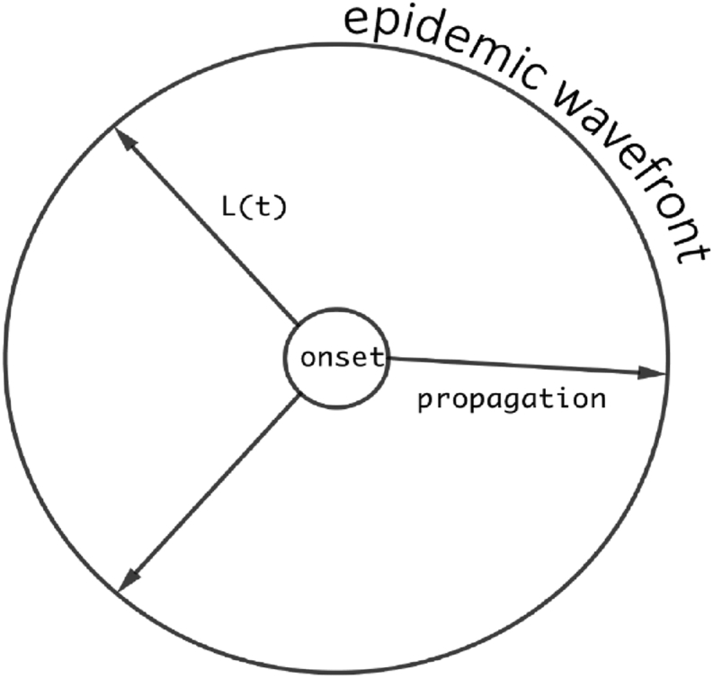
A schematic for a radially symmetrical epidemic propagation.

With the radial symmetry, system (2.2) is reduced to

$$\begin{array}{cc}& \frac{\partial S}{\partial t}+\frac{1}{r}\frac{\partial }{\partial r}(rVS)=\mathrm{\Gamma }-{\beta }_{E}SE-{\beta }_{I}SI,\\ & \frac{\partial E}{\partial t}+\frac{1}{r}\frac{\partial }{\partial r}(rVE)={\beta }_{E}SE+{\beta }_{I}SI-\alpha E,\\ & \frac{\partial I}{\partial t}+\frac{1}{r}\frac{\partial }{\partial r}(rVI)=\alpha E-(w+\gamma )I,\\ & \frac{\partial R}{\partial t}+\frac{1}{r}\frac{\partial }{\partial r}(rVR)=\gamma I.\end{array}$$ (2.5)

Adding up the equations in (2.5) and using equation (2.4), we obtain the following equation for the velocity V which characterizes the epidemic flow in our setting:

$$\frac{1}{r}\frac{\partial }{\partial r}\left(rV\right)=\mathrm{\Gamma }(t,r)-wI(t,r),0<r\le L,t\ge 0.$$ (2.6)

A trivial case corresponds to V = 0 for 0 < r ≤ L and t ≥ 0, which would reduce the PDE system (2.5) to a normal SEIR model based on ODEs. In what follows we assume that Γ(t, r) − wI(t, r) ≠ 0, which would hold for a small w > 0 in particular, to ensure a nontrivial velocity field. The kinematic condition applied to the moving boundary L(t) yields

$$\frac{dL}{dt}=V(t,L).$$ (2.7)

Since L(t) represents the spatial spread of the epidemic, we naturally expect that V(t, L) ≥ 0, which indicates that the expansion rate of the epidemic domain O(t) (i.e., the domain that contains all the individuals who have been infected) is non-negative. This is also a reflection of the fact that the number of the cumulative infected cases is always non-decreasing. Finally, at the center r = 0, the radial symmetry implies that

$$V(t,0)=0.$$ (2.8)

Equations (4.3), (4.6) constitute a spatial epidemic model with a moving boundary, which is our focus in this study. We will discuss related initial and boundary conditions in Section 4.

3. Simplified models and analyses

Even though the model (2.5) has only one space variable r, it is a strongly coupled nonlinear PDE system with a moving boundary and an unknown velocity field, which makes mathematical analysis difficult. Nevertheless, we may gain useful insight by examining some simplified models that reduce the original PDE system to ODE systems.

We first consider the scenario when all the time derivatives in system (2.5) vanish; i.e., all the population densities reach a steady state: S = S(r), E = E(r), I = I(r), and R = R(r). Also assume Γ = Γ(r). Then system (2.5) becomes

$$\begin{array}{cc}& \frac{1}{r}\frac{\partial }{\partial r}(rVS)=\mathrm{\Gamma }(r)-{\beta }_{E}SE-{\beta }_{I}SI,\\ & \frac{1}{r}\frac{\partial }{\partial r}(rVE)={\beta }_{E}SE+{\beta }_{I}SI-\alpha E,\\ & \frac{1}{r}\frac{\partial }{\partial r}(rVI)=\alpha E-(w+\gamma )I,\\ & \frac{1}{r}\frac{\partial }{\partial r}(rVR)=\gamma I,\end{array}$$ (3.1)

and equation (2.6) becomes

$$\frac{1}{r}\frac{\partial }{\partial r}(rV)=\mathrm{\Gamma }(r)-wI(r)≔B(r).$$ (3.2)

Clearly, the velocity field V is also independent of time; i.e., V = V(r), with the boundary condition V(0) = 0 based on equation (2.8). Consequently, equation (3.2) can be integrated to obtain

$$V\left(r\right)=\frac{1}{r}{\int }_0^{r}uB\left(u\right)du,0<r\le L.$$ (3.3)

It can be easily verified that lim_r→0V(r) = 0 based on equation (3.3). Meanwhile, equation (2.7) becomes

$$\frac{dL}{dt}=V(L)=\frac{1}{L}{\int }_0^{L}uB(u)du.$$ (3.4)

Equations (3.1), (3.2), (3.4) form ODE systems which can be easily solved numerically. If we substitute equation (3.2) into system (3.1), we obtain

$$\begin{array}{cc}& V\frac{dS}{dr}=\mathrm{\Gamma }(r)-{\beta }_{E}SE-{\beta }_{I}SI-SB(r),\\ & V\frac{dE}{dr}={\beta }_{E}SE+{\beta }_{I}SI-\alpha E-EB(r),\\ & V\frac{dI}{dr}=\alpha E-(w+\gamma )I-IB(r),\\ & V\frac{dR}{dr}=\gamma I-RB(r).\end{array}$$ (3.5)

Essential properties of system (3.5) are determined by its equilibria, which represent the spatially homogeneous solutions of the system. Standard equilibrium analysis can be conducted to investigate such properties.

Before we analyze system (3.5), however, let us present another important scenario of the PDE system (2.5), which is concerned with uniform spatial distribution of the population densities so that they are only dependent on time: S = S(t), E = E(t), I = I(t), and R = R(t). Assume also that Γ = Γ(t). System (2.5) is then reduced to

$$\begin{array}{cc}& \frac{dS}{dt}+\frac{S}{r}\frac{\partial }{\partial r}(rV)=\mathrm{\Gamma }(t)-{\beta }_{E}SE-{\beta }_{I}SI,\\ & \frac{dE}{dt}+\frac{E}{r}\frac{\partial }{\partial r}(rV)={\beta }_{E}SE+{\beta }_{I}SI-\alpha E,\\ & \frac{dI}{dt}+\frac{I}{r}\frac{\partial }{\partial r}(rV)=\alpha E-(w+\gamma )I,\\ & \frac{dR}{dt}+\frac{R}{r}\frac{\partial }{\partial r}(rV)=\gamma I.\end{array}$$ (3.6)

Meanwhile, equation (2.6) becomes

$$\frac{1}{r}\frac{\partial }{\partial r}(rV)=\mathrm{\Gamma }(t)-wI(t)≔B(t).$$ (3.7)

Equation (3.7) yields

$$V(t,r)=\frac{1}{2}B\left(t\right)r,0\le r\le L,t\ge 0.$$ (3.8)

Equation (3.8) shows that even though the state variables (S, E, I and R) are spatially independent, the velocity field depends on both the time and space, and an explicit expression for V(t, r) can be obtained. Evaluating the solution (3.8) at r = L and substituting the result into equation (2.7), we obtain

$$L\left(t\right)=L\left(0\right)e^{\frac{1}{2}{\int }_0^{t}B\left(u\right)du},t\ge 0.$$ (3.9)

Substituting equation (3.7) into system (3.6), we obtain

$$\begin{array}{cc}& \frac{dS}{dt}=\mathrm{\Gamma }(t)-{\beta }_{E}SE-{\beta }_{I}SI-SB(t),\\ & \frac{dE}{dt}={\beta }_{E}SE+{\beta }_{I}SI-\alpha E-EB(t),\\ & \frac{dI}{dt}=\alpha E-(w+\gamma )I-IB(t),\\ & \frac{dR}{dt}=\gamma I-RB(t).\end{array}$$ (3.10)

Comparing systems (3.5) and (3.10), we observe that the two systems share the same (constant) equilibria, which are referred to as the spatially homogeneous stationary solutions. These solutions represent the spatially homogeneous states for system (3.5), and the temporally stationary states for system (3.10). In particular, there is always a unique disease-free equilibrium for the two systems:

$$(S,E,I,R)=(1,0,0,0).$$ (3.11)

We may gain more detailed information on the constant equilibrium solutions of system (3.5) or (3.10) on a special case when Γ is a constant. Using the next-generation matrix technique (van den Driessche & Watmough, 2002), we can derive the basic reproduction number of (3.10) as

$${\mathcal{R}}_0=\frac{{\beta }_E}{\mathrm{\Gamma }+\alpha }+\frac{\alpha {\beta }_I}{(\mathrm{\Gamma }+\alpha )(w+\gamma +\mathrm{\Gamma })},$$ (3.12)

where the two parts represent the contributions from the exposed individuals and infected individuals, respectively, in shaping the transmission risk of the disease. Based on the classical stability theory for epidemic models (van den Driessche & Watmough, 2002), the disease-free equilibrium is stable when ${\mathcal{R}}_0<1$, and is unstable when ${\mathcal{R}}_0>1$.

Now we investigate the existence of a non-trivial equilibrium (S∗, E∗, I∗, R∗), also referred to as an endemic equilibrium. Setting the right-hand side of each equation in (3.10) to 0 and substituting the expression of B(t), we obtain

$$\begin{array}{c}\mathrm{\Gamma }-{\beta }_{E}SE-{\beta }_{I}SI-S(\mathrm{\Gamma }-wI)=0,\\ {\beta }_{E}SE+{\beta }_{I}SI-\alpha E-E(\mathrm{\Gamma }-wI)=0,\\ \alpha E-(w+\gamma )I-I(\mathrm{\Gamma }-wI)=0,\\ \gamma I-R(\mathrm{\Gamma }-wI)=0.\end{array}$$ (3.13)

The third equation in (3.13) yields

$$E=\frac{w+\gamma +\mathrm{\Gamma }}{\alpha }I+\frac{w}{\alpha }{I}^2≔F(I).$$ (3.14)

Adding the first two equations in (3.13) and substituting equation (3.14), we obtain

$$S=\frac{\alpha F(I)-\mathrm{\Gamma }}{wI-\mathrm{\Gamma }}-F(I)≔G(I).$$ (3.15)

Substituting equations (3.14), (3.15) into the second equation in (3.13), we obtain an equation on a single variable I:

$$P(I)=F(I),$$ (3.16)

where

$$P(I)≔\frac{\left[{\beta }_{E}F(I)+{\beta }_{I}I\right]G(I)+wIF(I)}{\alpha +\mathrm{\Gamma }}.$$ (3.17)

We proceed to analyze the roots of equation (3.16), which will determine the equilibrium points of system (3.10). It is straightforward to observe that F(0) = 0 and P(0) = 0. Thus, the two curves F(I) and P(I) have an intersection at I = 0, which corresponds to the disease-free equilibrium. Meanwhile, we have

$$F^{\prime }(I)=\frac{w+\gamma +\mathrm{\Gamma }}{\alpha }+\frac{2w}{\alpha }I\mathrm{a}\mathrm{n}\mathrm{d}{F}^{\prime }(0)=\frac{w+\gamma +\mathrm{\Gamma }}{\alpha }.$$ (3.18)

By differentiating the function P, we have

$$P^{\prime }(I)=\frac{1}{\alpha +\mathrm{\Gamma }}\left[\left({\beta }_{E}F(I)+{\beta }_{I}I\right)G^{\prime }(I)+\left({\beta }_E{F}^{\prime }(I)+{\beta }_I\right)G(I)+wF(I)+wI{F}^{\prime }(I)\right],$$ (3.19)

where

$$G^{\prime }(I)=\left(\frac{\alpha }{wI-\mathrm{\Gamma }}-1\right)F^{\prime }(I)-\frac{w\left[\alpha F(I)-\mathrm{\Gamma }\right]}{{(wI-\mathrm{\Gamma })}^2}.$$ (3.20)

Since F(0) = 0 and G(0) = 1, equation (3.19) yields

$$P^{\prime }(0)=\frac{{\beta }_E{F}^{\prime }(0)+{\beta }_I}{\alpha +\mathrm{\Gamma }}.$$ (3.21)

Furthermore,

$$\begin{array}{cc}{P}^{″}(I)=\frac{1}{\alpha +\mathrm{\Gamma }}[& \left({\beta }_{E}F(I)+{\beta }_{I}I\right)G^{″}(I)+2\left({\beta }_E{F}^{\prime }(I)+{\beta }_I\right)G^{\prime }(I)+{\beta }_E{F}^{″}(I)G(I)\\ & +2w{F}^{\prime }(I)+wI{F}^{″}(I)].\end{array}$$ (3.22)

By our assumption, we are considering a small disease induced mortality rate; i.e., w ≪ 1. When w = 0, it can be easily verified that F′(I) > 0, F″(I) = 0, G′(I) < 0, G″(I) = 0, and, consequently, $P^{″}(I)=\frac{2}{\alpha +\mathrm{\Gamma }}\left[{\beta }_E{F}^{\prime }(I)+{\beta }_I\right]G^{\prime }(I)<0$. By continuity, when w is sufficiently small, we also have P″(I) < 0, so that the curve represented by P(I) is concave. On the other hand, the curve F(I) is always convex since F″(I) = 2w/α ≥ 0 for any w ≥ 0.

We already know that P(0) = F(0) = 0. Moreover, through direct algebraic manipulation, we can verify that when w < Γ, we have P(1) < F(1); i.e., when I = 1, the curve P(I) is below the curve F(I). Therefore, the two curves have an intersection at some I∗ ∈ (0, 1) if and only if P′(0) > F′(0). Due to the different concavities of the two curves, such an intersection must be unique if it exists. Using equations (3.18) and (3.21), we can easily obtain that

$$P^{\prime }(0)>F^{\prime }(0)\mathrm{i}\mathrm{f}\mathrm{a}\mathrm{n}\mathrm{d}\mathrm{o}\mathrm{n}\mathrm{l}\mathrm{y}\mathrm{i}\mathrm{f}{\mathcal{R}}_0>1,$$ (3.23)

where ${\mathcal{R}}_0$ is defined in equation (3.12). Hence, we conclude that when Γ is a constant and w is small, there is a unique positive equilibrium (S∗, E∗, I∗, R∗) for system (3.10) if and only if ${\mathcal{R}}_0>1$. This equilibrium corresponds to a non-trivial, spatially homogeneous stationary solution for the original PDE system (2.5).

To examine the stability of the endemic equilibrium (S∗, E∗, I∗, R∗), we look at the Jacobian matrix of system (3.10). Since the first three equations in (3.10) do not depend on the variable R, we only need to check these three equations in terms of S, E and I. When w = 0, the Jacobian matrix at the endemic equilibrium is given by

$$J^{\ast }=\left[\begin{array}{ccc}-({\beta }_E{E}^{\ast }+{\beta }_I{I}^{\ast }+\mathrm{\Gamma })& -{\beta }_E{S}^{\ast }& -{\beta }_I{S}^{\ast }\\ {\beta }_E{E}^{\ast }+{\beta }_I{I}^{\ast }& {\beta }_E{S}^{\ast }-(\alpha +\mathrm{\Gamma })& {\beta }_I{S}^{\ast }\\ 0& \alpha & -(\gamma +\mathrm{\Gamma })\end{array}\right].$$ (3.24)

Using the Routh-Hurwitz stability criterion and the algebraic relationship in (3.13), we can directly verify that all the three eigenvalues of the characteristic polynomial associated with the matrix J∗ have negative real parts. This property also holds when w is sufficiently small due to the continuous dependence on the parameter. Hence, the positive equilibrium of system (3.10) is locally asymptotically stable for small w > 0.

Therefore, our equilibrium analysis concludes that for the steady-state system (3.5) or the spatially invariant system (3.10), with constant influx Γ and small disease-induced death rate w, there is a forward transcrtical bifurcation taking place: when ${\mathcal{R}}_0<1$, solutions locally converge to the disease-free equilibrium (1, 0, 0, 0); when ${\mathcal{R}}_0>1$, solutions locally converge to the endemic equilibrium (S∗, E∗, I∗, R∗). These two equilibria represent two spatially homogeneous steady states for the PDE system (2.5), one indicating the elimination of the disease and the other indicating the persistence of the disease.

Finally, suppose that when ${\mathcal{R}}_0>1$ the endemic equilibrium is reached at t = t∗, then the function B = Γ − wI≔B∗ becomes a constant. Consequently, equation (3.8) yields

$$V=V\left(r\right)=\frac{1}{2}{B}^{\ast }r,0\le r\le L,t\ge t^{\ast },$$ (3.25)

and equation (3.9) yields

$$L\left(t\right)=L\left(t^{\ast }\right)e^{\frac{1}{2}{B}^{\ast }(t-t^{\ast })},t\ge t^{\ast },$$ (3.26)

which shows that the radius L(t) would increase exponentially with a constant rate $\frac{1}{2}{B}^{\ast }$ for t ≥ t∗. The same result can be obtained from equations (3.3), (3.4). Note that equation (3.4) leads to $dL/dt=\frac{1}{2}{B}^{\ast }L$.

4. Numerical simulation

For the original PDE system (2.5), we will focus on a numerical study. One challenge in dealing with the proposed model is that it involves an unknown moving boundary L(t) which has to be determined as part of the solution procedure. To overcome this difficulty, we make the following coordinate transformation (t, r) → (τ, z):

$$\tau =t,z=\frac{r}{L(t)}.$$ (4.1)

Under this transformation, the original variable domain 0 ≤ r ≤ L(t) is mapped to a fixed domain 0 ≤ z ≤ 1. It is straightforward to calculate the partial derivatives under the transformed coordinates:

$$\frac{\partial }{\partial t}=\frac{\partial }{\partial \tau }-\frac{z{L}^{\text{'}}\left(\tau \right)}{L\left(\tau \right)}\frac{\partial }{\partial z},\frac{\partial }{\partial r}=\frac{1}{L\left(\tau \right)}\frac{\partial }{\partial z}.$$ (4.2)

Hence, the equations in system (2.5) are mapped to the following equations

$$\begin{array}{cc}& \frac{\partial S}{\partial \tau }+\frac{V-z{L}^{\prime }(\tau )}{L}\frac{\partial S}{\partial z}=\mathrm{\Gamma }(\tau ,z)-{\beta }_{E}SE-{\beta }_{I}SI-SA,\\ & \frac{\partial E}{\partial \tau }+\frac{V-z{L}^{\prime }(\tau )}{L}\frac{\partial E}{\partial z}={\beta }_{E}SE+{\beta }_{I}SI-\alpha E-EA,\\ & \frac{\partial I}{\partial \tau }+\frac{V-z{L}^{\prime }(\tau )}{L}\frac{\partial I}{\partial z}=\alpha E-(w+\gamma )I-IA,\\ & \frac{\partial R}{\partial \tau }+\frac{V-z{L}^{\prime }(\tau )}{L}\frac{\partial R}{\partial z}=\gamma I-RA,\end{array}$$ (4.3)

for τ ≥ 0 and 0 ≤ z ≤ 1, where A = Γ(τ, z) − wI(τ, z). Meanwhile, equation (2.6) becomes

$$\frac{1}{zL}\frac{\partial }{\partial z}\left(zV\right)=A=\mathrm{\Gamma }-wI,0<z\le 1,\tau \ge 0.$$ (4.4)

The kinematic condition (2.7) becomes

$$\frac{dL}{d\tau }=V(\tau ,1),$$ (4.5)

and the boundary condition (2.8) becomes

$$V(\tau ,0)=0.$$ (4.6)

A numerical procedure can be naturally developed with standard methods for PDEs (Thomas, 1995). Using the initial conditions (see equation (4.10)), equation (4.4) can be solved to obtain the initial profile of the velocity V. At each time step τ_n+1, equation (4.5) is solved to update L(τ_n+1). Then S, E, I and R are computed from equation (4.3). Note that

$$\frac{V(\tau ,z)-z{L}^{\prime }(\tau )}{L}=0\mathrm{a}\mathrm{t}z=0\mathrm{a}\mathrm{n}\mathrm{d}z=1,$$ (4.7)

based on equations (4.5), (4.6). Hence, no boundary conditions are needed to handle system (4.3). Instead, at z = 0 and z = 1, an ODE system is solved to update S, E, I and R at the two boundary points. Next, equation (4.4) is computed to update the velocity V. This would complete one computational cycle and the procedure repeats at the next time step.

Using the mapped equations and the afore-mentioned numerical procedure, we now present several numerical tests to validate our models and analyses presented in previous sections.

We first consider a special form of Γ(t, z) that represents a constant influx for the susceptible population:

$$\mathrm{\Gamma }(t,z)=\mathrm{\Gamma }=\mathrm{C}\mathrm{o}\mathrm{n}\mathrm{s}\mathrm{t}.$$ (4.8)

Note that since τ = t, we will use t to refer to the time variable in the remainder of this section. We have conducted some mathematical analysis in Section 3 on the simplified models based on ODEs. Now we run numerical simulation to the original PDE model to test the different scenarios associated with the spatially homogeneous stationary states. To start the numerical simulation, we set up a small circular disk as the initial epidemic domain and assume uniform distribution of human hosts within this initial domain. We then examine different values of the basic reproduction number ${\mathcal{R}}_0$, defined in equation (3.12) for the spatially homogeneous ODE system (3.10), by varying the constant influx Γ. Specifically, we fix all the other model parameters, and pick different values of Γ so that ${\mathcal{R}}_0<1$ and ${\mathcal{R}}_0>1$ can be achieved. For each case, we numerically simulate the original PDE model based on the formulation in equations (4.3), (4.6).

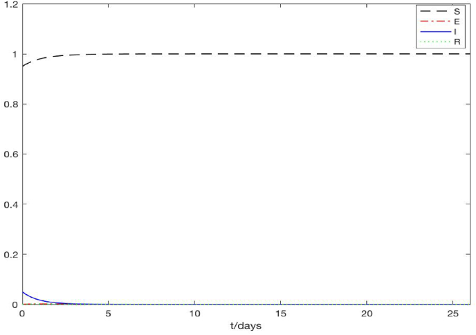
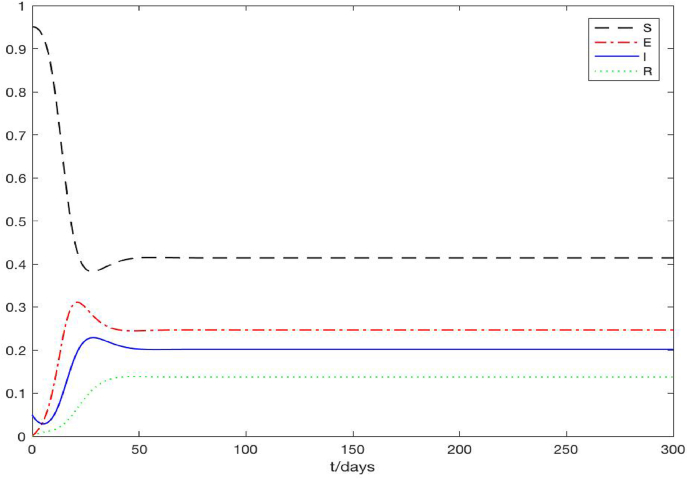
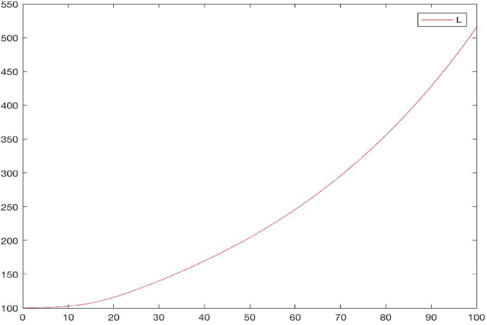
Fig. 2 shows a typical scenario for ${\mathcal{R}}_0<1$, where we set Γ = 1 person per meter per day which leads to ${\mathcal{R}}_0\approx 0.45$. We observe that the density of the susceptible individuals quickly approach a steady state at S = 1, while the densities of the exposed, infected and recovered individuals all approach 0. Thus, the solutions converge to the disease-free equilibrium (S, E, I, R) = (1, 0, 0, 0), and this pattern is uniform for all the spatial positions. For illustration, Fig. 2 only displays the result at z = 0.5, but the results are the same for all 0 ≤ z ≤ 1 in the spatial domain. Fig. 3 shows a typical scenario for ${\mathcal{R}}_0>1$, where we set Γ = 0.1 person per meter per day which results in ${\mathcal{R}}_0\approx 2.39$. We clearly see that after 50 days, all the solution curves level off at a positive steady state, referred to as the endemic equilibrium, where (S, E, I, R) ≈ (0.41, 0.25, 0.20, 0.14). Again we present the result at z = 0.5, but the pattern is identical for all the spatial points. These results are consistent with our analytical predictions in Section 3. In addition, Fig. 4 displays the evolution of the radius L with respect to time t, under the same parameter setting as in Fig. 3. The exponential growth of L(t) after t > 50, when the endemic equilibrium of the state variables is reached, can be clearly observed. This behavior agrees with our analytical result in equation (3.26).

Fig. 2.

A typical scenario showing that solutions of the PDE system converge to the disease-free equilibrium (S, E, I, R) = (1, 0, 0, 0) when ${\mathcal{R}}_0<1$.

Fig. 3.

A typical scenario showing that solutions of the PDE system converge to the positive endemic equilibrium (S∗, E∗, I∗, R∗) when ${\mathcal{R}}_0>1$.

Fig. 4.

A typical scenario showing the exponential growth of the radius L(t) when ${\mathcal{R}}_0>1$.

Next, we perform a case study with more practical relevance, to illustrate the potential of this model for real-world applications. At present, COVID-19 remains a global pandemic. The hundreds of millions of infections caused by COVID-19, the worldwide spread of this disease, and its huge impact on public health and the world economy, are all unprecedented. Here we simulate a scenario that could partially represent the COVID-19 outbreak in Wuhan, China, the first epicenter for the coronavirus disease.

To implement the model, we consider the following form of the influx Γ with both temporal and spatial dependence:

$$\mathrm{\Gamma }(t,z)=cz\left[1-S(t,z)\right],t\ge 0,0\le z\le 1.$$ (4.9)

By our definition of the epidemic domain, there is no infection outside the domain O(t) at time t. Equation (4.9) assumes that all the individuals outside the epidemic disk O(t) are susceptible with a (normalized) uniform density of 1, and that the increment of the susceptible density is linearly distributed along the radial direction.

The following initial setting is considered. We set January 23, 2020 as day 0, when the Chinese government ordered to lock down Wuhan city. We assume that at t = 0 the infection takes place at a small neighborhood of the origin z = 0, represented by a small circular disk with a radius ϵ > 0. We also assume that a small number of infections are present inside this domain, represented by a (normalized) density θ > 0. We further assume that there are no exposed and recovered individuals initially and the human individuals within this domain are uniformly distributed at t = 0. Thus the initial conditions for these variables are given by

$$L(0)=ϵ,S(0,z)=1-\theta ,E(0,z)=0,I(0,z)=\theta ,R(0,z)=0.$$ (4.10)

Values of the model parameters are provided in Table 1. These parameter values are based on the reported data and previous modeling studies for COVID-19 in Wuhan. Note that, however, the two transmission rates β_E and β_I have been normalized by the total population size in Wuhan City; it is estimated that about 9 million people remained in the city by January 23, 2020 (The government of Wuhan h). The Huanan Seafood Market, a live animal and seafood wholesale market in Wuhan, was widely believed as a primary source and onset location of the epidemic (Li et al., 2020; Yang and Wang, 2020b). The initial epidemic domain in our model would represent the area occupied by this seafood market. The market has a reported floor space of about 50, 000 square meters, though the actual area covered by the market would be less than that considering the presence of multi-storey buildings in the market. Hence, we set the radius of the initial epidemic disk as ϵ ≈ 100 m. It is reported that 55% of the first 425 confirmed cases were linked to this marketplace (Li et al., 2020). Within our initial epidemic domain, we set the percentage of infection as θ ≈ 5%.

Table 1.

Definitions and values of model parameters.

Parameter	Definition	Value	Source
βE	Transmission rate between S and E	0.347 m per day per person	(Tang et al., 2020; Yang and Wang, 2020b)
βI	Transmission rate between S and I	0.112 m per day per person	(Tang et al., 2020; Yang and Wang, 2020b)
α	Incubation rate	1/7 per day	Spencer et al. (1101)
w	Disease-induced death rate	0.01 per day	(The government of Wuhan h)
γ	Recovery rate	1/15 per day	Spencer et al. (1101)
θ	Percentage of the initial density of I	5%	(Li et al., 2020; The government of Wuhan h)
ϵ	Initial radius of the epidemic domain	100 m	(The government of Wuhan h)
c	Constant in the influx Γ	1200 per day	Assumed

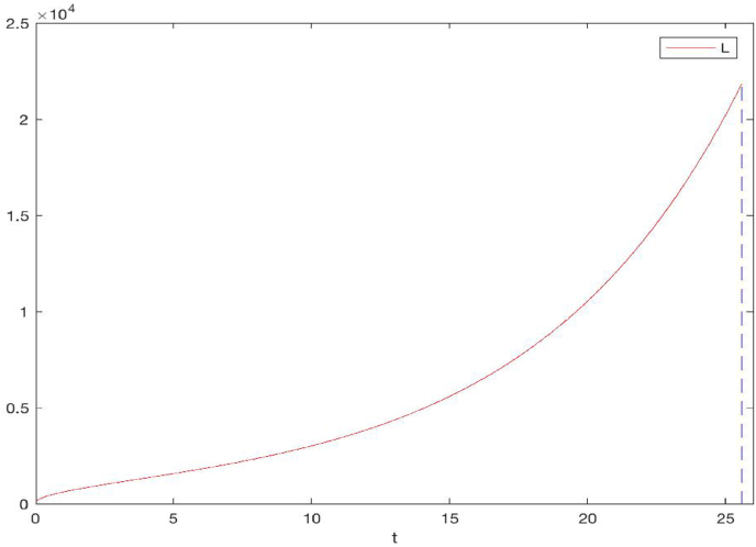
Wuhan City has an urban area of 1528 square kilometers (Wikipedia: Wuhan. Availab). When L(t) = 22 km, the area of the epidemic domain O(t) would approximately equal that of the entire city of Wuhan. Our simulation result for the time evolution of the radius L(t) is shown in Fig. 5, where we observe that L(t) reaches the threshold value L∗ = 22 km at t ≈ 25.6 days. Since day 0 in our model corresponds to January 23, 2020, our result indicates that by February 17, 2020, the epidemic had spread to the entire city of Wuhan. For this epidemic (perhaps also for most other epidemics), the specific day and time that the infection had spread to the entire city were unknown. Nevertheless, based on the reported COVID-19 data (Yang & Wang, 2021; The government of Wuhan h), the number of cumulative cases in Wuhan was exponentially increasing for the first 25–28 days (i.e., from January 23 to February 16–19, 2020), and then the rate of increase slowed down afterwards. Meanwhile, according to a study on the spread of COVID-19 to places surrounding Wuhan City (You, Wu, Yang, Liu, & Liu, 2020), a number of cities, towns and villages near Wuhan started reporting a sharp increase for the number of cases during the period of February 10–19, 2020. These patterns of reported data seems to be consistent with our numerical estimate of the growth of the epidemic domain, which is approximated as a regular circular disk in this study.

Fig. 5.

The growth of the radius L(t) for the COVID-19 epidemic in Wuhan, China. L(t) reaches 22 km at t ≈ 25.6 days (marked by the vertical dashed line), when the epidemic domain O(t) covers the entire city of Wuhan.

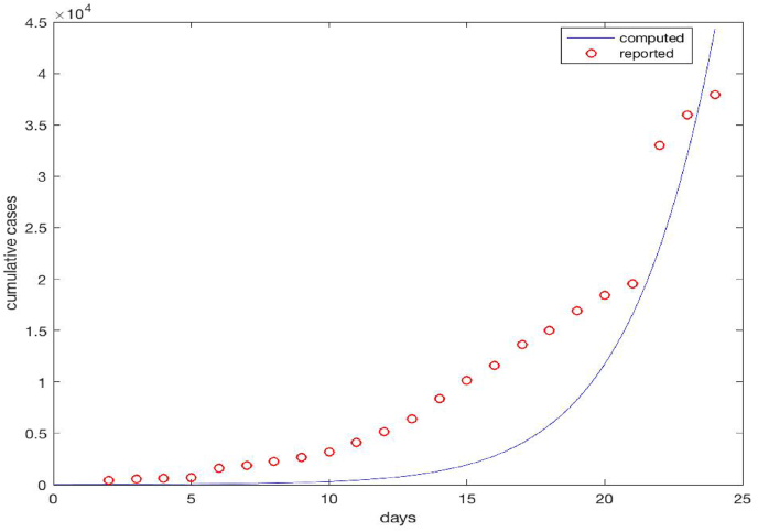
Fig. 6 shows our simulation results for the number of cumulative cases, in comparison to the daily reported data. Based on our model, the number of cumulative cases at time t is computed as

$${\int }_0^{1}I(t,z)dz+{\int }_0^{1}R(t,z)dz+{\int }_0^t{\int }_0^{1}wI(s,z)dzds,$$ (4.11)

where the first integral represents the number of individuals who are currently infected, the second integral represents the number of individuals who have recovered, and the third integral represents the number of individuals who have died from the infection, at time t. Compared to the reported data, our simulation results generally underestimate the number of cases. Note that we have not employed any data fitting method in this simulation. Another possible reason could be our (simplistic) assumption that the epidemic starts and spreads from a single location. In reality, there were initial cases reported in a number of different places in the Wuhan region (Du, Javan, Nugent, Cowling, & Meyers, 2020; Li et al., 2020; You et al., 2020), all of which would contribute to the spread of the COVID-19 epidemic.

Fig. 6.

The cumulative confirmed cases for the COVID-19 epidemic in Wuhan. The circles represent the reported data on a daily basis, and the solid line represents the simulation results.

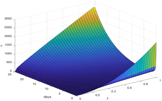
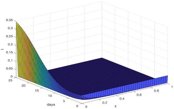
Fig. 7 shows a three-dimensional plot for the velocity field V(t, z) versus time and space. We observe that V generally increases with t and z. Meanwhile, Fig. 8 shows a three-dimensional plot for the density of infected individuals I versus time and space. We observe that the infection level remains significant and increases with time near the center of the epidemic domain (z = 0) which, by our assumption, is the onset site for the outbreak. For the majority of the spatiotemporal domain, however, the infection density (or, equivalently, the percentage of infected individuals among the whole population) appears low, due to the large population size (about 9 million) in the city of Wuhan.

Fig. 7.

Three-dimensional plot of the velocity V versus time and space for the COVID-19 epidemic in Wuhan.

Fig. 8.

Three-dimensional plot of the density of infected individuals I versus time and space for the COVID-19 epidemic in Wuhan.

5. Discussion

Predicting the spatial spread of an infectious disease has been one of the most important tasks in epidemic management and public health administration. Although a large number of mathematical, statistical and computational models have been developed for this purpose, their applications to realistic epidemic scenarios have not met our expectation. In particular, the outbreak and worldwide spread and persistence of COVID-19 underscore the gap between the complexity of epidemic spreading and our current quantitative understanding in epidemiology.

As a pilot effort, we have presented a new PDE-based epidemic modeling framework that involves a moving boundary, with a focus on the spatial spread of the infectious disease. We have introduced a time-dependent epidemic domain in our model, where its moving boundary represents the wave front of the epidemic that is determined by the speed of the human movement. By modeling the collective human movement as a convection process, our study is primarily macroscopic, treating the human population as one or more homogeneous classes, without paying special attention to the individual heterogeneities. In this sense, our approach is built on the classical compartmental, population-level models of mathematical epidemiology. Our major innovation, however, is to introduce a moving-boundary problem into the epidemic modeling, where both the epidemic domain and the velocity field are unknown and have to be determined as part of the solution.

Our proposed model explicitly accounts for the interplay between disease transmission, host movement, and epidemic spread, in order to gain deeper insight into the realistic spread of an epidemic in space and its impact on the epidemic progression and evolution. On the other hand, we have kept our mathematical model sufficiently simple, involving a minimal number of equations and parameters, so that it can be possibly applied to the simulation of realistic epidemics. In this work, we have illustrated a potential application of our model by incorporating the COVID-19 data from Wuhan City in China. Our modeling results in this proof of concept provide useful information on the spatial spread of COVID-19 in Wuhan during the first period of the pandemic.

There are a number of limitations in this pilot study. Our model does not represent the detailed mobility patterns of the human hosts. Practically, the movement of individual hosts could be highly heterogeneous and would be better described by an agent-based model. We have introduced a simple deterministic formulation that human hosts move in the radial direction described by a convective velocity field, which makes the analysis and simulation more tractable than that for an agent-based model. We may extend the current modeling framework by incorporating diffusion terms that represent the random component in the motion of human hosts. On the other hand, the model may be unrealistic by assuming that all individuals at the same location move with the same speed. In particular, severely infected individuals may be hospitalized and isolated and may not be able to freely move. Our focus is the collective behavior of human movement that determines the propagation of the epidemic wave, and the velocity field should be understood as the average speed of the human movement. Moreover, we have not utilized any parameter fitting techniques in our numerical simulation, including the application to the COVID-19 epidemic in Wuhan, which may have impacted the quality of our simulation results in comparison to the reported number of cases. Based on this initial effort of model development, we plan to incorporate data fitting, which is a non-trivial task for any PDE-based epidemic models, in our future efforts to improve the accuracy of our model predictions and to enable more realistic applications. Additionally, we may improve our modeling work by using the more general 2D formulation presented in Section 2, and by incorporating multiple epidemic onset locations into our model setting.

Declaration of competing interest

Both authors, Qiao Zhuang and Jin Wang, declare that there is no conflict of interest in this work.

Handling editor: Dr Lou Yijun

References

- Allen L.J.S., Bolker B.M., Lou Y., Nevai A.L. Asymptotic profiles of the steady states for an SIS epidemic patch model. SIAM Journal on Applied Mathematics. 2007;67:1283–1309. [Google Scholar]
- Allen L.J.S., Bolker B.M., Lou Y., Nevai A.L. Asymptotic profiles of the steady states for an SIS epidemic reaction-diffusion model. Discrete and Continuous Dynamical Systems. 2008;21:1–20. [Google Scholar]
- Arino J., van den Driessche P. A multi-city epidemic model. Mathematical Population Studies. 2003;10:175–193. [Google Scholar]
- Attard P. Oxford University Press; 2012. Non-equilibrium thermodynamics and statistical mechanics: Foundations and applications. [Google Scholar]
- Bertozzi A.L., Franco E., Mohler G., Short M.B., Sledge D. The challenges of modeling and forecasting the spread of COVID-19. Proceedings of the National Academy of Sciences. 2020;117(29):16732–16738. doi: 10.1073/pnas.2006520117. [DOI] [PMC free article] [PubMed] [Google Scholar]
- Bertuzzo E., Casagrandi R., Gatto M., Rodriguez-Iturbe I., Rinaldo A. On spatially explicit models of cholera epidemics. Journal of The Royal Society Interface. 2010;7:321–333. doi: 10.1098/rsif.2009.0204. [DOI] [PMC free article] [PubMed] [Google Scholar]
- Brauer F. Mathematical epidemiology: Past, present, and future. Infectious Disease Modelling. 2017;2(2):113–127. doi: 10.1016/j.idm.2017.02.001. [DOI] [PMC free article] [PubMed] [Google Scholar]
- Brauer F., Castillo-Chavez C. Springer; New York: 2001. Mathematical models in population biology and epidemiology. [Google Scholar]
- Brauer F., Castillo-Chavez C., Feng Z. Challenges, opportunities and theoretical epidemiology. Mathematical Models in Epidemiology. 2019;69:507–531. [Google Scholar]
- Cantrell R.S., Cosner C. The effects of spatial heterogeneity in population dynamics. Journal of Mathematical Biology. 1991;29:315–338. [Google Scholar]
- Cantrell R.S., Cosner C. Wiley; 2003. Spatial ecology via reaction-diffusion equations. [Google Scholar]
- Capasso V. Vol. 97. Springer-Verlag; Berlin: 1993. (Mathematical structures of epidemic systems, lecture notes in biomathematics). [Google Scholar]
- Chan J.F.-W., Yuan S., Kok K.-H., To K., Chu H., Yang J. A familial cluster of pneumonia associated with the 2019 novel coronavirus indicating person-to-person transmission: A study of a family cluster. Lancet. 2020;395:514–523. doi: 10.1016/S0140-6736(20)30154-9. [DOI] [PMC free article] [PubMed] [Google Scholar]
- Chowell G., Sattenspiel L., Bansal S., Viboud C. Mathematical models to characterize early epidemic growth: A review. Physics of Life Reviews. 2016;18:66–97. doi: 10.1016/j.plrev.2016.07.005. [DOI] [PMC free article] [PubMed] [Google Scholar]
- Cosner C., Beier J.C., Cantrell R.S., Impoinvil D., Kapitanski L., Potts M.D. The effects of human movement on the persistence of vector-borne diseases. Journal of Theoretical Biology. 2009;258:550–560. doi: 10.1016/j.jtbi.2009.02.016. [DOI] [PMC free article] [PubMed] [Google Scholar]
- Diekmann O., Heesterbeek J.A.P. Wiley; New York: 2000. Mathematical epidemiology of infectious diseases. [Google Scholar]
- van den Driessche P., Watmough J. Reproduction numbers and sub-threshold endemic equilibria for compartmental models of disease transmission. Mathematical Biosciences. 2002;180:29–48. doi: 10.1016/s0025-5564(02)00108-6. [DOI] [PubMed] [Google Scholar]
- Du Z., Javan E., Nugent C., Cowling B.J., Meyers L.A. Using the COVID-19 to influenza ratio to estimate early pandemic spread in Wuhan, China and Seattle, US. EClinicalMedicine. 2020;26:100479. doi: 10.1016/j.eclinm.2020.100479. [DOI] [PMC free article] [PubMed] [Google Scholar]
- Gaff H.D., Gross L.J. Modeling tick-borne disease: A metapopulation model. Bulletin of Mathematical Biology. 2007;69:265–288. doi: 10.1007/s11538-006-9125-5. [DOI] [PubMed] [Google Scholar]
- The government of Wuhan homepage. Available at: http://english.wh.gov.cn/.
- Grenfell B.T., Dobson A.P., editors. Ecology of infectious diseases in natural populations. Cambridge University Press; 1995. [Google Scholar]
- Hanski I. Oxford University Press; 1999. Metapopulation ecology. [Google Scholar]
- Hasibeder G., Dye C. Population dynamics of mosquito-borne disease: Persistence in a completely heterogeneous environment. Theoretical Population Biology. 1988;33:31–53. doi: 10.1016/0040-5809(88)90003-2. [DOI] [PubMed] [Google Scholar]
- Hethcote H.W. The mathematics of infectious diseases. SIAM Review. 2000;42:599–653. [Google Scholar]
- Hsieh Y.-H., van den Driessche P., Wang L. Impact of travel between patches for spatial spread of disease. Bulletin of Mathematical Biology. 2007;69:1355–1375. doi: 10.1007/s11538-006-9169-6. [DOI] [PMC free article] [PubMed] [Google Scholar]
- Kopell N., Howard L.N. Target pattern and spiral solutions to reaction-diffusion equations with more than one space dimension. Advances in Applied Mathematics. 1981;2:417–449. [Google Scholar]
- Kot M. Cambridge University Press; Cambridge: 2001. Elements of mathematical ecology. [Google Scholar]
- Levins R. Some demographic and genetic consequences of environmental heterogeneity for biological control. Bulletin of the Entomological Society of America. 1969;15(3):237–240. [Google Scholar]
- Li Q., Guan X., Wu P., Wang X., Zhou L., Tong Y. Early transmission dynamics in Wuhan, China, of novel coronavirus-infected pneumonia. New England Journal of Medicine. 2020;382:1199–1207. doi: 10.1056/NEJMoa2001316. [DOI] [PMC free article] [PubMed] [Google Scholar]
- Li T., Li Y., Hethcote H.W. Periodic traveling waves in SIRS endemic models. Mathematical and Computer Modelling. 2009;49:393–401. [Google Scholar]
- Magal P., Webb G.F., Wu Y. On the basic reproduction number of reaction-diffusion epidemic models. SIAM Journal on Applied Mathematics. 2019;79:284–304. [Google Scholar]
- Metz J.A.J., van den Bosch F. In: Epidemic models: Their structure and relation to data. Mollison D., editor. Cambridge University Press; 1996. Velocities of epidemic spread. [Google Scholar]
- Murray J.D. Springer; 2002. Mathematical biology. [Google Scholar]
- Rass L., Radcliffe J. Vol. 102. American Mathematical Society; 2003. (Spatial deterministic epidemics, mathematical surveys and monographs). [Google Scholar]
- Riley S., Eames K., Isham V., Mollison D., Trapman P. Five challenges for spatial epidemic models. Epidemics. 2015;10:68–71. doi: 10.1016/j.epidem.2014.07.001. [DOI] [PMC free article] [PubMed] [Google Scholar]
- Rodriguez D.J., Torres-Sorando L. Models for infectious diseases in spatially heterogeneous environments. Bulletin of Mathematical Biology. 2001;63:547–571. doi: 10.1006/bulm.2001.0231. [DOI] [PubMed] [Google Scholar]
- Ruan S., Wang W., Levin S.A. The effect of global travel on the spread of SARS. Mathematical Biosciences and Engineering. 2006;3:205–218. doi: 10.3934/mbe.2006.3.205. [DOI] [PubMed] [Google Scholar]
- J.A. Spencer, D.P. Shutt, S.K. Moser, H. Clegg, H.J. Wearing, H. Mukundan, and C.A. Manore, Epidemiological parameter review and comparative dynamics of influenza, respiratory syncytial virus, rhinovirus, human coronvirus, and adenovirus. DOI: 10.1101/2020.02.04.20020404. [DOI]
- Tang B., Wang X., Li Q., Bragazzi N.L., Tang S., Xiao Y. Estimation of the transmission risk of 2019-nCoV and its implication for public health interventions. Journal of Clinical Medicine. 2020;9(2):462. doi: 10.3390/jcm9020462. [DOI] [PMC free article] [PubMed] [Google Scholar]
- Thieme H.R. Princeton University Press; Princeton: 2003. Mathematics in population biology. [Google Scholar]
- Thieme H.R. Spectral bound and reproduction number for infinite-dimensional population structure and time heterogeneity. SIAM Journal on Applied Mathematics. 2009;70:188–211. [Google Scholar]
- Thomas J.W. Springer-Verlag; New York: 1995. Numerical partial differential equations: Finite difference methods. [Google Scholar]
- Wang X., Gao D., Wang J. Influence of human behavior on cholera dynamics. Mathematical Biosciences. 2015;267:41–52. doi: 10.1016/j.mbs.2015.06.009. [DOI] [PMC free article] [PubMed] [Google Scholar]
- Wang W., Zhao X.-Q. Basic reproduction numbers for reaction-diffusion epidemic models. SIAM Journal on Applied Dynamical Systems. 2012;11:1652–1673. [Google Scholar]
- Wikipedia: Wuhan. Available at: http://en.wikipedia.org/wiki/Wuhan.
- Wu J. In: Brauer F., van den Driessche P., Wu J., editors. Vol. 1945. Springer; 2008. Spatial structure: Partial differential equations models. (Mathematical epidemiology, lecture notes in mathematics). [Google Scholar]
- Yang C., Wang J. Basic reproduction numbers for a class of reaction-diffusion epidemic models. Bulletin of Mathematical Biology. 2020;82:111. doi: 10.1007/s11538-020-00788-x. [DOI] [PMC free article] [PubMed] [Google Scholar]
- Yang C., Wang J. A mathematical model for the novel coronavirus epidemic in Wuhan, China. Mathematical Biosciences and Engineering. 2020;17(3):2708–2724. doi: 10.3934/mbe.2020148. [DOI] [PMC free article] [PubMed] [Google Scholar]
- Yang C., Wang J. Transmission rates and environmental reservoirs for COVID-19 – a modeling study. Journal of Biological Dynamics. 2021;15(1):86–108. doi: 10.1080/17513758.2020.1869844. [DOI] [PMC free article] [PubMed] [Google Scholar]
- You M., Wu Z., Yang Y., Liu J., Liu D. Spread of coronavirus 2019 from Wuhan to rural villages in the Hubei Province. Open Forum Infectious Diseases. 2020;7(7):ofaa228. doi: 10.1093/ofid/ofaa228. [DOI] [PMC free article] [PubMed] [Google Scholar]