Gut inference: A computational modelling approach

Abstract

Neurocomputational theories have hypothesized that Bayesian inference underlies interoception, which has become a topic of recent experimental work in heartbeat perception. To extend this approach beyond cardiac interoception, we describe the application of a Bayesian computational model to a recently developed gastrointestinal interoception task completed by 40 healthy individuals undergoing simultaneous electroencephalogram (EEG) and peripheral physiological recording. We first present results that support the validity of this modelling approach. Second, we provide a test of, and confirmatory evidence supporting, the neural process theory associated with a particular Bayesian framework (active inference) that predicts specific relationships between computational parameters and event-related potentials in EEG. We also offer some exploratory evidence suggesting that computational parameters may influence the regulation of peripheral physiological states. We conclude that this computational approach offers promise as a tool for studying individual differences in gastrointestinal interoception.

1. Introduction

There is growing interest in understanding the neural basis of interoception, with an emerging literature on both theoretical models and empirical studies (Berntson & Khalsa, 2021; Bonaz et al., 2021; Chen et al., 2021; Petzschner, Garfinkel, Paulus, Koch, & Khalsa, 2021; Quigley, Kanoski, Grill, Barrett, & Tsakiris, 2021; Weng et al., 2021). Aside from basic science interests, interoception has also become an important topic of mental health research, with evidence for abnormalities in depression, anxiety, eating, and substance use disorders, among others (reviewed in (Khalsa et al., 2018)). Theoretical work within neuroscience and psychiatry has articulated plausible neurocomputational accounts of interoceptive processing (Allen, Levy, Parr, & Friston, 2019; Barrett & Simmons, 2015; Owens, Allen, Ondobaka, & Friston, 2018; Owens, Friston, Low, Mathias, & Critchley, 2018; Paulus, Feinstein, & Khalsa, 2019; Petzschner, Weber, Gard, & Stephan, 2017; Seth, 2013; Seth & Critchley, 2013; Smith, Thayer, Khalsa, & Lane, 2017; Stephan et al., 2016), largely extending from leading Bayesian models of exteroceptive (Bastos et al., 2012; Friston, 2005), cognitive (Chen, Takahashi, Nakagawa, Inoue, & Kusumi, 2015; Clark, Watson, & Friston, 2018; Friston, Stephan, Montague, & Dolan, 2014; Huys, Maia, & Frank, 2016; Montague, Dolan, Friston, & Dayan, 2012; Moutoussis, Shahar, Hauser, & Dolan, 2017; Parr & Friston, 2018; Schwartenbeck & Friston, 2016; Sharp & Eldar, 2019), emotional (Hesp, Smith, Allen, Friston, & Ramstead, 2020; Smith, Lane, Parr, & Friston, 2019; Smith, Parr, & Friston, 2019), and motor control domains (Adams, Perrinet, & Friston, 2012; Adams, Shipp, & Friston, 2013; Edwards, Adams, Brown, Pareés, & Friston, 2012). A few studies have also tested predictions of Bayesian computational models and fit such models to behavioral data on interoception tasks in both healthy and psychiatric samples (Petzschner et al., 2019; Smith, Kuplicki, Feinstein et al., 2020; Smith, Kuplicki, Teed, Upshaw, & Khalsa, 2020; Harrison et al., 2021).

The most common paradigms for studying interoception within psychological research settings have traditionally focused on heartbeat perception (for a review see (Khalsa & Lapidus, 2016)). However, cardiac perception is generally quite poor, with only roughly 35% of individuals accurately perceiving their own heartbeats at rest (Khalsa & Lapidus, 2016). Using heartbeats as task stimuli also presents unique challenges, as their intensity and timing cannot be tightly controlled in the absence of a pharmacological perturbation (Cameron & Minoshima, 2002; Khalsa, Rudrauf, Sandesara, Olshansky, & Tranel, 2009). The predominant focus on cardiac interoception is understandable given the ease with which this signal can be measured, but the limitations of certain heartbeat perception tasks have been raised repeatedly in recent years (Corneille, Desmedt, Zamariola, Luminet, & Maurage, 2020; Desmedt, Luminet, & Corneille, 2018; Murphy et al., 2018; Phillips, Jones, Rieger, & Snell, 1999; Ring & Brener, 2018; Ring, Brener, Knapp, & Mailloux, 2015; Windmann, Schonecke, Frohlig, & Maldener, 1999; Zamariola, Maurage, Luminet, & Corneille, 2018); but see (Ainley, Tsakiris, Pollatos, Schulz, & Herbert, 2020)). Other major reasons for the heavy utilization of cardiac interoception measures in psychological research include the inaccessibility of the body’s interior and the lack of (and difficulty designing) minimally invasive tasks to assess other modalities.

In a recent study we described a new method for studying gastrointestinal (GI) interoception that made use of mechanosensory stimulation via an ingestible vibrating capsule (Mayeli et al., 2021). Using an instruction set similar to heartbeat tapping paradigms, participants were asked to press a button whenever they felt a vibration sensation in their stomach. However, unlike heartbeats, the vibration timing and intensity could be precisely controlled. As an initial validation, we showed that standard signal detection measures could capture interesting behavioral and perceptual patterns in the data and that the vibrations reliably elicited electroencephalogram (EEG) event-related potential (ERPs) in a manner that was sensitive to vibration intensity. In the present study, we extend this work by applying a Bayesian computational modelling approach to this data, which we previously developed for a heartbeat tapping paradigm (Smith, Kuplicki, Feinstein et al., 2020; Smith, Kuplicki, Teed et al., 2020). This approach has the advantage of being able to capture learning dynamics that cannot be measured by signal detection approaches, as well as interactions between Bayesian beliefs about the precision of afferent GI signals (interoceptive precision; IP) and prior expectations. Successfully estimating these parameters could provide information of potential clinical relevance to conditions in which GI symptoms play a primary role.

In this paper we also provide a direct test of recently proposed neural process theories within the Bayesian framework known as active inference (Friston, FitzGerald, Rigoli, Schwartenbeck, & Pezzulo, 2017; Friston, Parr, & de Vries, 2017; Parr & Friston, 2018; Smith, Friston, & Whyte, 2021). Active inference postulates that ERP amplitudes are positively associated with the rate of change in beliefs in response to sensory stimuli. Therefore, if a sensory signal is expected to be reliable (high precision), it should be associated with larger ERPs (i.e., due to a faster evidence accumulation rate). Active inference also postulates a hierarchical structure in which higher-level (e.g., frontal) brain regions convey signals downward to sensory cortices – providing sensory processing with prior beliefs about what will be perceived. Here, if prior beliefs predict a sensation, then the presentation of a congruent stimulus should generate smaller ERPs, because beliefs do not need to change as much to account for the new observation. A primary means of learning in Bayesian models occurs through updating prior beliefs over slower timescales – where these slower-timescale processes are predicted to occur in higher brain regions (Kiebel, Daunizeau, & Friston, 2008; Murray et al., 2014; Smith, Steklis, Steklis, Weihs, & Lane, 2020). A large literature in computational neuroscience and psychiatry has also shown that individuals differ in the magnitude with which their prior beliefs are updated after each new observation (i.e., differences in learning rate; e.g., see (Browning, Behrens, Jocham, O’Reilly, & Bishop, 2015; Chen et al., 2015; Huang, Thompson, & Paulus, 2017; Smith, Schwartenbeck et al., 2020)). Thus, in addition to basic validation analyses, we tested the specific hypotheses that: 1) higher interoceptive precision (IP) values would be associated with stronger ERPs in sensory processing regions (i.e., parieto-occipital leads sensitive to capsule vibrations in our previous study), and 2) learning rates – which constrain the magnitude of change in prior beliefs after each observation – would modulate the amplitude of ERPs in the hierarchically higher frontal regions associated with these slower-timescale processes. We also expected that 3) more precise prior expectations to feel a vibration would be associated with attenuated ERPs when a vibration occurs.

2. Materials and methods

2.1. Participants

40 healthy volunteers between the ages of 18 and 40 years (mean =22.9, standard deviation (SD) = 4.56; 21 male and 19 female, mean body mass index (BMI) = 24.18, SD = 3.03) were recruited from the general community within and surrounding Tulsa, Oklahoma through electronic and print advertisements. Participants completed structured medical and psychiatric screening evaluations including the MINI (Mini-International Neuropsychiatric Interview) (Sheehan et al., 1998). Exclusion criteria included current pregnancy, testing positive for drugs of abuse (as defined by a urine screen during screening and during the study visit), a current diagnosis of a psychiatric disorder based on the MINI (Sheehan et al., 1998), past or present diagnosis of a significant gastrointestinal disorder, gastrointestinal surgery, a respiratory, cardiovascular, renal, hepatic, biliary or endocrine disease, as well as chronic use of psychotropic medications or non-steroidal anti-inflammatory drugs. The study was conducted at the Laureate Institute for Brain Research and the study protocol was approved by the Western Institutional Review Board (IRB). All participants provided written informed consent and they received financial compensation for participation.

2.2. Vibrating capsule

The study protocol asked individuals to swallow a capsule that would generate potentially perceivable vibration sensations while in the stomach before passing through the digestive tract. The vibrating capsule was developed by Vibrant Ltd (Israel) and is under investigation as a non-pharmacologic therapeutic option for chronic constipation using delivery of stimulation in the colon. It consists of an orally administered non-biodegradable capsule that is wirelessly activated using an activation base unit (Fig. 1). The safety of this approach has been established in both healthy human volunteers (Ron et al., 2015) and in patients with chronic constipation (Nelson et al., 2017; Rao, Lembo, Chey, Friedenberg, & Quigley, 2020). The Vibrant capsule is a non-significant risk device (NSR).

Fig. 1.

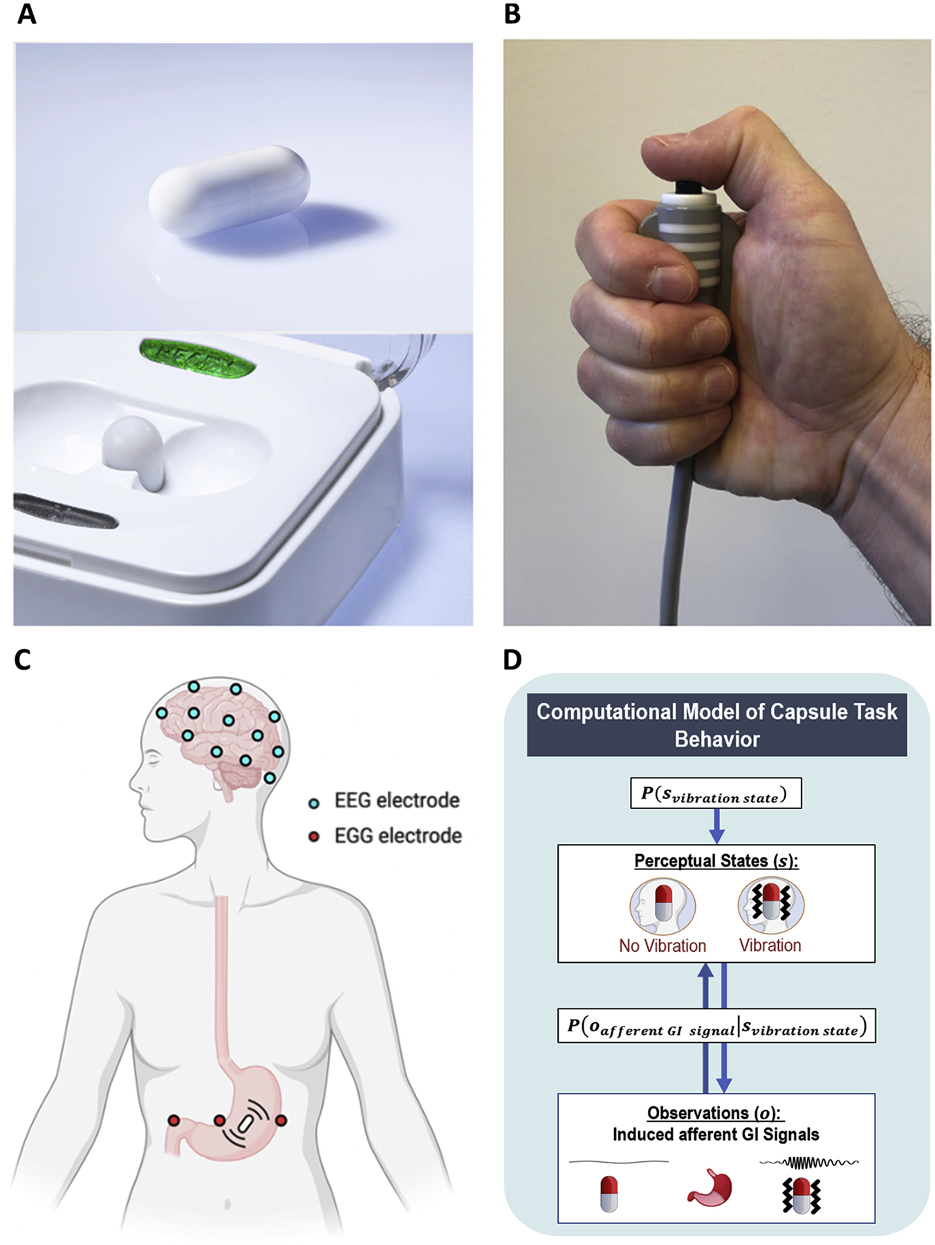
A) Vibrating capsule and activation base. B) The push button which participants were asked to press as soon as they detected a capsule-induced stomach sensation. C) Scalp electroencephalogram (EEG) and stomach electrogastrogram (EGG) lead placement. Additional collected peripheral physiological measures included electrocardiogram and skin conductance. D) Heuristic depiction of computational (Bayesian) model of task behavior.

2.3. Masking procedure

Participants were told that two different modes of the Vibrant capsule were being evaluated, and that they would be randomly assigned to one of three arms of the study (capsule mode A, capsule mode B, or a placebo capsule that did not vibrate). This was done to minimize demand characteristics (i.e., expectations that they should perceive vibrations during the experiment). Participants were further informed that neither they nor the experimenter would know the assigned condition. However, each participant in fact received a capsule that delivered vibratory stimulations, making this a single-blinded protocol. Participants were instructed to begin fasting (defined as no food or drink) for 3 h prior to the study visit to ensure that the contents of the stomach were empty at the time of capsule ingestion.

2.4. Mechanosensory stimulation

Capsules were activated by placing them in the base unit. Immediately after activation, participants swallowed the capsule with approximately 240 mL of water, while seated in a chair. After ingestion, participants were asked to pay attention to their stomach sensations while resting their eyes on a fixation cross displayed on a monitor approximately 60 cm away. Participants were instructed to use their dominant hand to press and hold a button each time they felt a sensation that they ascribed to the capsule, and to release the button once the vibration sensation ceased (Fig. 1). Vibrations began approximately 3 min after capsule activation in the base unit. Participants remained seated throughout the experiment to minimize movement artifact in the EEG and electrogastrogram (EGG) signals. They were told to rest their non-dominant hand in their lap and avoid palpating their abdomen. Throughout the experiment they were visually observed by a research assistant seated behind them to verify alertness and compliance with instructions.

In the experiment, each participant received two blocks of vibratory stimulation (normal and enhanced stimulation level) in counterbalanced order (19 received the normal block first, 21 received the enhanced block first). The normal condition entailed the delivery of a standard level of mechanosensory stimulation (as developed by Vibrant) consistent with the level of stimulation delivered during chronic constipation trials targeting the colon. The enhanced condition entailed delivery of an increased level of mechanosensory stimulation that was expected to facilitate gastrointestinal perception. Each block included a total of 60 stimulations (with each stimulation being 3 s in duration), which were delivered in a pseudorandom order (i.e., pseudorandom inter-vibration intervals ranging between 6 and 23 s) across a 13-minute period. After a 4-minute pause, a second round of 60 stimulations were delivered in pseudorandom order during a second 13-minute period (resulting in a 33-minute period of participation following capsule ingestion). This timing ensured that the capsule remained in the stomach during stimulations, since the normal gastric emptying time is estimated to be approximately 30 min (Benini et al., 2004; Bluemel et al., 2017; Diamanti et al., 2003). Due to a technical error, 3 vibrations failed to occur in the enhanced vibration block (irrespective of counterbalancing).

2.5. Vibration detection

A digital stethoscope (Thinklabs One, Thinklabs Inc., USA) was gently secured against the surface of the lower right quadrant of the abdomen using a Tegaderm patch (15 × 20 cm, 3M Inc., USA) to precisely verify the vibration timing. The associated signal was continuously recorded during the entire experiment at a sampling rate of 1000 Hz and fed into the physiological recording software. We developed custom analysis scripts in Matlab (version 2019b, Mathworks, Inc.) to confirm the timing of each vibration, including a two-step procedure to detect their onset and offset. In the first step, the script identified the vibration timings automatically using the “findchangepts” function in Matlab. In the second step, the timing for each vibration was double-checked manually and adjusted if needed (see our prior report for more details; (Mayeli et al., 2021)).

2.6. Physiological recordings

Electroencephalogram (EEG) signals were recorded continuously using a 32-channel EEG system from Brain Products GmbH (Munich, Germany). The EEG cap consisted of 32 channels, including references, arranged according to the international 10–20 system. One of these channels recorded the electrocardiogram (ECG) signal via an electrode placed on the participant’s back, leaving 31 EEG signals available for analysis. The online reference for EEG recording was electrode FCz. The EEG signal was acquired with a 0.2 millisecond (ms) temporal resolution (i.e., 16-bit 5,000 Hz sampling), and a measurement resolution of 0.1 microvolts (μV).

Electrogastrogram (EGG) signals were recorded continuously using a Biopac MP150 Acquisition Unit (Biopac Inc., USA) and running Acknowledge software version 4.4.2 at a sampling rate of 1000 Hz. Two active abdominal electrodes positioned below the left costal margin and between the xyphoid process and umbilicus were utilized to capture cutaneous EGG signals. The reference electrode was positioned in the right upper quadrant in line with the others (Dirgenali, Kara, & Okkesim, 2006).

The same Biopac MP150 Acquisition Unit was used to record the skin conductance response (SCR) and ECG at a sampling rate of 1000 Hz. SCR was recorded via two gel-filled electrodes placed on the thenar and hypothenar eminences of the nondominant palm. The ECG signal was obtained using two electrodes positioned in a lead-2 placement. All physiological recordings were screened for artifacts (e.g., motion) and analyzed offline using AcqKnowledge version 4.4.2 and Matlab version 2019b. A 30-minute eyes open period of recording preceded the capsule ingestion for baseline estimation of resting peripheral physiological (EGG, ECG, and SCR) parameters.

2.7. EEG data processing

All pre- and post-processing of EEG data was completed using BrainVision Analyzer 2 software (Brain Products GmbH, Munich, Germany). Data was downsampled to 250 Hz. Next, a fourth order Butterworth (i.e., 24 dB/octave roll off) band-rejection filter (1 Hz bandwidth) was applied to remove alternating current (AC) power line noise (60 Hz). Then, a bandpass filter between 0.1 and 80 Hz (eighth order Butterworth Filter, 48 dB/octave roll off) was utilized to filter out signals unrelated to brain activity. Infomax independent component analysis (ICA) was then applied for independent component decomposition (Bell & Sejnowski, 1995) over the entire data length, after excluding intervals with excessive motion-artifact. ICA was run on the data from 31 EEG channels yielding 31 independent components (ICs). The timecourse signal, power spectrum density, topographic map, and energy of these ICs were utilized to detect and remove artifactual ICs (i.e., muscle, ocular, and single channel artifacts) (Mayeli, Zotev, Refai, & Bodurka, 2016). Additional steps were also applied to identify the ERP signals (see Mayeli et al., 2019). The data was first segmented from the 200 ms prior to each vibration to the 3000 ms post onset of each vibration, allowing baseline correction to the average of the 200 ms interval preceding the vibration onset. Next, EEG data was re-referenced to the average of the mastoid channels (TP9 and TP10). Automated procedures were then applied to detect bad intervals and flatlining in the data. Bad intervals were defined as those with any change in amplitude between data points that exceeded 50 μv or absolute fluctuations exceeding 200 μV in any 200 ms interval of the segments (i.e., −200 to 3000 ms); flatlining was defined as any change of less than 0.5 μV in a 200 ms period. Trials that included any of these artifacts were excluded. Based on initial inspection of the ERP waveform, there was a prominent late positive deflection in the ERP signal peaking around 600 ms and lasting up to 3000 ms (see Fig. 6 in results section below). To capture the peak of this response, for each electrode we measured the response to a vibration as the mean amplitude of activation from 300 to 600 ms after vibration onset (i.e., starting on the downward slope of this deflection and continuing to include its maximum amplitude) relative to a baseline value defined by the average of the EEG signal 200 ms prior to onset. Although much less pronounced, further inspection suggested there was also a negative deflection within an earlier window peaking around 150 ms in certain electrodes. To capture this response, for each electrode we measured the response to a vibration as the mean amplitude of activation from 100 to 176 ms (this choice of time window was also informed by contrasts of the normal vs. enhanced stimulation blocks in our previous study; see (Mayeli et al., 2021) for further details). We therefore also examined the possibility of a relationship between computational parameters and responses within this early time window.

Fig. 6.

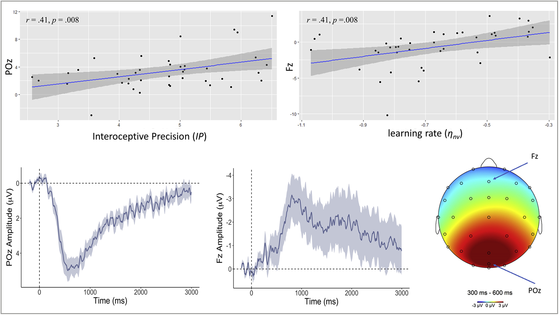
Upper left: Scatterplot depicting the relationship between (log-transformed) interoceptive precision (IP) estimates and the average amplitude of the ERP waveform elicited by capsule vibration for a representative parieto-occipital electrode (POz; between 300–600 ms post-vibration). Bottom left: ERP waveform (mean ± SE) elicited by vibration in POz. Upper right and lower middle panels depict analogous results for a representative frontal electrode (Fz) and (log-transformed) learning rate from the absence of vibrations (η_nv) – reflecting how quickly prior expectations decrease in precision during the periods (of relative length) between vibrations. Bottom right: Late positive potential topography across the scalp between 300 and 600 ms window after the vibration onset relative to the 200 ms pre-stimulus baseline across the scalp and across the entire task. Positive deflections were elicited in posterior cortices, while deflections approach neutral and negative values when moving toward more anterior electrodes. Positive ERP values are inverted (vice versa for negative values) per convention.

2.8. Peripheral physiological data processing

The single-channel EGG recording from each participant was divided into baseline (pre-stimulus), normal, and enhanced windows based on the counterbalanced protocol. For each window, the spectral power was computed to identify the location with the largest activity in the normogastria range (2.5–3.5 cycle per minute (cpm)). The spectral power analysis retained peaks of frequency in each condition for each participant. Fast Fourier Transform (FFT) from the FieldTrip toolbox version 2020-12-02 (Oostenveld, Fries, Maris, & Schoffelen, 2011) was utilized to estimate the spectral power with a Hanning taper to reduce spectral leakage and control frequency smoothing. To further characterize the gastric rhythm, we adopted a finite impulse response (FIR) filter to filter the EGG signal into low frequency ranges. FIR copes very well with very low frequency filtering (as shown in (Wolpert, Rebollo, & Tallon-Baudry, 2020)). Then, a Hilbert transform was applied to compute the instantaneous phase and amplitude envelope of the gastric rhythm. To further account for bad segments in the data, we used the artifact detection method described in (Wolpert et al., 2020). This method relies on the regularity of the computed cycle durations (the SD of cycle duration from the condition). More specifically, a segment was considered an artifact if either 1) the cycle length was greater than the mean ± SD of the cycle length distribution, or 2) the cycle showed a non-monotonic change in phase. Following the decision tree approach, any cycles with either of these conditions was considered as an artifact and excluded. The power spectral analysis was calculated again after excluding bad segments from the EGG signal, including subsequent filtering. Here we report the absolute power for each of four gastric ranges: normogastria (2.5–3.5 cpm), tachygastria (3.75–9.75 cpm), bradygastria (0.5–2.5 cpm), and total power (0.5–11 cpm) (in line with (Vianna & Tranel, 2006)).

Data from ECG recordings were used to compute the average phasic heart rate change in beats per minute (BPM) in response to each vibration. This was done by computing the BPM for the 3 s after each vibration onset relative to the 3 s prior to each vibration. Specifically, the peaks of the R-waves were used to estimate heart rate from ECG recordings for pre-stimulus and stimulus segments (a custom peak detection algorithm in Matlab was used for peak detection), and the difference in heart rate between the 3-second stimulus segment and 3-second pre-stimulus segment was used to derive the vibration-induced heart rate response. As a control condition, for ECG recordings during the pre-task resting baseline period we generated a series of 60 pseudo-events with 30-second intervals within the 30-minute baseline period (after ignoring the first 2 min to allow for reaching a physiological steady state) and calculated the same response metric. To assess tonic heart rate levels, we additionally estimated the overall heart rate for each block.

SCR was estimated using Continuous Deconvolution Analysis (CDA) implemented in the Ledalab Toolbox version 3.4.9 (Bach, 2014). We assessed phasic changes from pre-stimulus to stimulus segments (3 s after each vibration onset relative to the 3 s prior) using the maximum value of the phasic activity (i.e., peak response amplitude) metric. For each block, we downsampled the signal to 20 Hz and applied a smoothing window of 200 ms after setting the threshold of significant events to 0.01 microSiemens (μS). As a control condition (similar to analyses of heart rate above), for SCR recordings during the pre-task resting baseline period we used the same pseudo-events from the baseline period to characterize changes in SCR relative to physiological rest.

2.9. Self-report measures

Participants completed several self-report surveys indexing potentially relevant state factors (including Visual Analog Scales with ratings from 0–100). Before the task they were asked:

“How hungry do you currently feel?” (0 = Not at all/none, 100 = Extremely, most I have ever felt).

“How thirsty do you currently feel?” (0 = Not at all/none, 100 = Extremely, most I have ever felt).

After the task they were asked:

“Overall, how pleasant/unpleasant did your body feel during the capsule stimulation?” (0 = Extremely unpleasant, 100 = Extremely pleasant)

“How would you describe your state of mind during the capsule stimulation?” (0 = Foggy/Unable to think clearly, 100 = Focused/Able to think with complete clarity)

“How difficult was it to detect the stomach sensations?” (0 = Very easy, 100 = Very difficult)

“How confident were you in your overall ability to accurately detect the capsule vibrations?” (0 = Not at all, 100 = Extremely)

These were adapted from scales we have previously developed and used in studies of cardiac interoception (e.g., see (Smith, Kuplicki, Feinstein et al., 2020; Smith, Feinstein et al., 2021)). Participants also completed other previously validated affective and interoceptive measures, including the Multidimensional Assessment of Interoceptive Awareness (MAIA; (Mehling et al., 2012)), Anxiety Sensitivity Index (ASI; (Sandin, Chorot, & McNally, 2001)), and Positive and Negative Affect Schedule (PANAS; (Watson, Clark, & Tellegen, 1988)). For a detailed description of these measures, see Supplementary Materials.

2.10. Computational modelling

Computational modelling plays a central role in our approach. Instead of just looking for differences or correlations between behavioral and physiological responses, we aim to explain these responses in terms of Bayesian belief updating induced by interoceptive signals. This requires us to model belief updating under ideal Bayesian observer assumptions – and then use empirical responses to estimate each individual’s prior beliefs, interoceptive precision, and learning rates. The use of ideal Bayesian observer models of this sort is sometimes referred to as computational phenotyping – and rests on a formal or first principle account of how people assimilate sensory information.

To quantify the belief updating that underlies task performance, we adopted a Bayesian computational modelling approach analogous to that used in recent heartbeat tapping paradigms (Smith, Kuplicki, Feinstein et al., 2020; Smith, Kuplicki, Teed et al., 2020). This model of perception was derived from a Markov decision process (MDP) formulation of active inference that has been used in previous work; for more details about the structure and mathematics of this class of (discrete state space) models, see (Friston, FitzGerald et al., 2017; Friston, Parr et al., 2017; Parr & Friston, 2017; Smith, Friston et al., 2021). For a graphical depiction of our model and the associated vectors and matrices, see Fig. 2, and further descriptions in Table 1. Matlab code used to build this model and fit parameters to behavioral data can also be accessed at https://github.com/rssmith33/Gut-Inference-Model-Scripts.

Fig. 2.

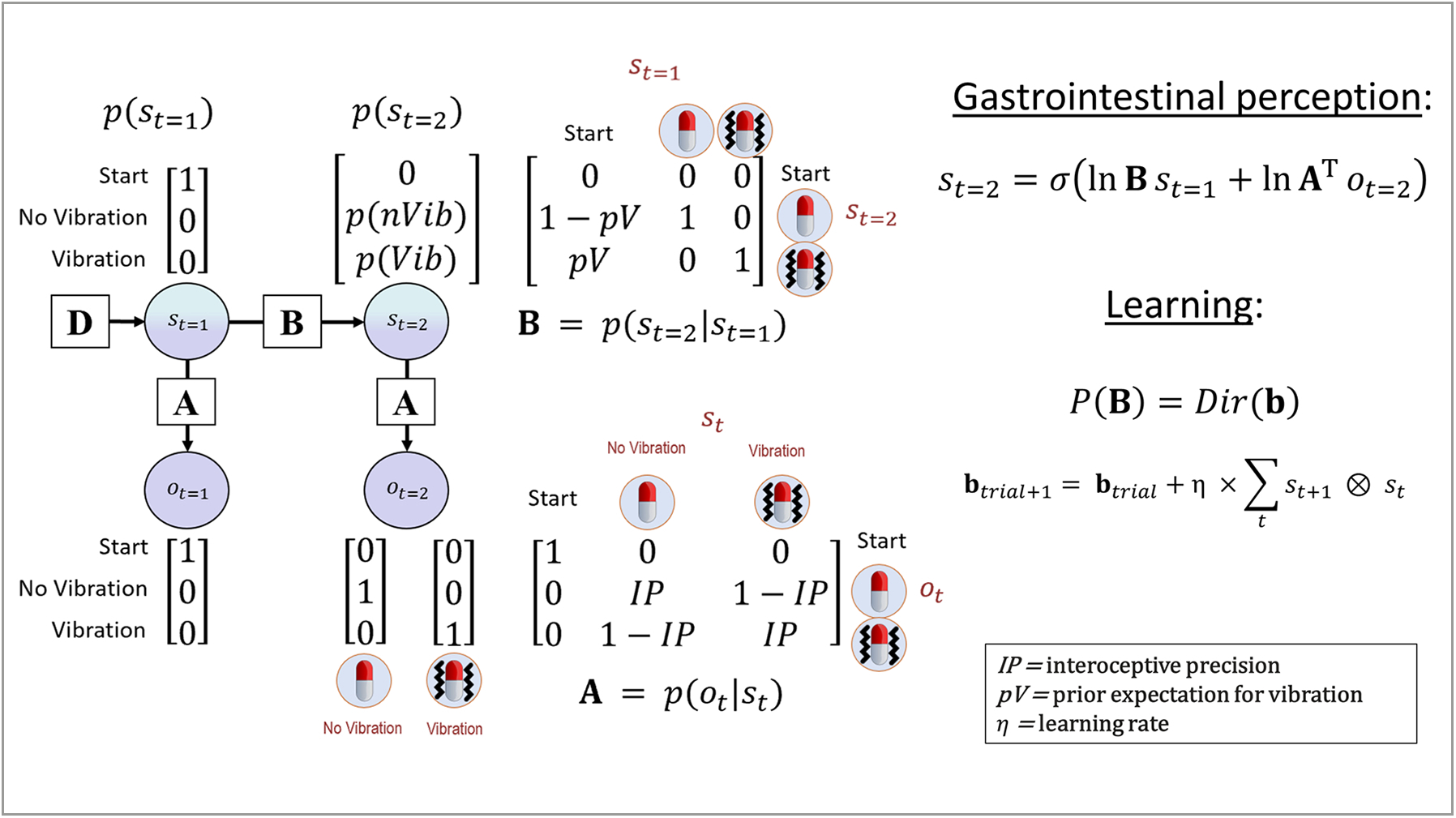
Bayesian approach used to model interoceptive awareness on the vibration detection task. The generative model is here depicted graphically, such that arrows indicate dependencies between variables. Associated vectors/matrices are also shown. At each timepoint (t), observations (o) depend on hidden states (s), where this relationship is specified by the A matrix, and those states depend on previous states (as specified by the B matrix), or on the initial states (with probabilities specified by the D vector). This model represents a simplified version of a commonly used active inference formulation of partially observable Markov decision processes (for more details regarding the structure and mathematics describing these models, see (Da Costa et al., 2020; Friston, Lin et al., 2017; Friston, FitzGerald et al., 2017; Smith, Friston et al., 2021)). In this model, the observations were no-vibration/vibration, and the hidden states included beliefs about the presence or absence of a vibration. Selection of the button press vs. no button press actions were sampled from the posterior distribution over states (p(s_t=2)) – that is, a higher posterior probability of a vibration state (p(Vib)) corresponded to a higher probability of choosing to push the button, and a higher posterior probability of the no-vibration state (p(nVib)) corresponded to a higher probability of choosing not to press the button. The model parameters we estimated corresponded to: 1) interoceptive precision (IP) – the precision of the mapping from true vibrations to beliefs about vibrations in the A matrix, which can be associated with the weight assigned to interoceptive prediction errors; 2) prior beliefs favoring the presence of a vibration (pV); and 3) a learning rate (η) that controls how quickly prior beliefs change after each observation (where distinct learning rates can be fit for when a vibration is vs. isn’t observed). On each trial, beliefs about the probability of a vibration (corresponding to the probability of choosing to press the button) relied on Bayesian inference as implemented in the “gastrointestinal perception” equation shown on the right of the figure, and changes in prior beliefs were controlled by the learning equation below this (explained in the main text). Note that the state variable s in these equations corresponds to posterior expectations. Each 3-second time period in which a vibration was or was not present was treated as a separate trial, in which the participant started in the “start” state and then updated beliefs about hidden states based on observation of a vibration (or no-vibration). For this reason, the pV parameter in the transition matrix (B) only specifies the probability of transitioning from the “start” state to the vibration vs. no-vibration states, and the vibration and no-vibration states simply have identity mappings (i.e., a given trial cannot transition between these two states).

Table 1.

Description of computational model elements.

Model variable	General definition	Model-specific description
t	Timepoint within a trial	There were 2 timepoints in each trial (i.e., for each 3-second time window). At t = 1, the participant was modelled as waiting to infer the presence or absence of a vibration in a “start” state. At t = 2, either a vibration or no-vibration observation was presented (depending on whether the time window for that trial contained a vibration or no-vibration), and a posterior probability of the presence vs. absence of a vibration was inferred. Note that t here refers to a participant’s beliefs about a timepoint in each trial. This means that before a participant makes their observation (i.e., when still in the “start” state), they have prior beliefs about the state at time t = 2, and these beliefs are then updated after the new observation.*
o t	Observable outcomes at time t	Outcomes: 1 Start 2 Vibration 3 No-vibration
s t	Posterior beliefs over hidden states at time t	Hidden states: 1 Start 2 Vibration 3 No-Vibration
A matrix p(ot|st)	A matrix encoding beliefs about the relationship between hidden states and observable outcomes (i.e., the probability that specific outcomes will be observed given specific hidden states).	Encodes beliefs about the relationship between vibration vs. no-vibration states and vibration vs. no-vibration observations. The precision of the relationship between vibration/no-vibration states and vibration/no-vibration observations is controlled by a parameter IP. This parameter specifies how much evidence a vibration observation (i.e., the vibration signal from the stomach) provides for a vibration state and how much evidence the absence of a vibration observation provides for a no-vibration state.
B matrix p(st+1|st)	A matrix encoding beliefs about how hidden states will evolve over time (transition probabilities).	Encodes the prior belief that either a vibration or no-vibration state would occur in each 3-second window, as controlled by a parameter pV.
D vector p(st=1)	A vector encoding beliefs about (a probability distribution over) initial hidden states.	This specifies that the individual always begins in an initial starting state.

^*Note that in the active inference literature these beliefs about timepoints are often instead denoted with the Greek letter tau (τ) in order to distinguish them from the times (t) at which new observations are presented (for details, see (Smith, Friston et al., 2021)). Although this technical point is not emphasized in the main text, it is what allows a participant’s beliefs about τ = 2 (presence or absence of a vibration) in our model to change from before (t = 1) to after (t = 2) making a new observation (i.e., from prior to posterior beliefs).

Observations (o) in the model were categorical and included no-vibration, vibration, and a “start” observation. Hidden states (s) in the model, which were inferred based on observations, were also categorical and included a no-vibration state, a vibration state, and a “start” state (i. e., the vibration observations corresponded to the ground truth, whereas vibration states corresponded to a participant’s perception). Each trial in the model corresponded to a 3-second time window during the task in which participants were told a vibration might be felt. Each trial formally had two timesteps (t = 1 and t = 2). At t = 1, the participant always formally began in the “start” state and made the associated “start” observation. At t = 2, the participant either made a no-vibration or vibration observation and inferred whether they had transitioned from the “start” state into the no-vibration or vibration state. In other words, they inferred a posterior distribution over states p(s_t=2) that assigned a probability to the no-vibration state and to the vibration state, where this posterior distribution was informed by 1) prior beliefs about the probability of transitioning from the “start” state to each of the two states, p(s_t=2|s_t=1), and 2) beliefs about the likelihood of making a no-vibration or vibration observation given the presence of the no-vibration or vibration state, p(o_t|s_t).

A vector D encoded prior beliefs over initial states, p(s_t=1), which specified that the participant always started the trial in the “start” state with a probability of 1 (see vector in upper left portion of the model depiction in Fig. 2). A matrix B encoded the probability that each state would transition into any other state:

$$B=p\left(s_{t+1}\mid s_t\right)=\left[\begin{array}{ccc}0& 0& 0\\ 1-pV& 1& 0\\ pV& 0& 1\end{array}\right]$$

Here, columns indicate (from left to right) the “start” state, the no-vibration state, and the vibration state at time t = 1, and rows (from top to bottom) indicate the “start” state, the no-vibration state, and the vibration state at time t = 2. The probability of transitioning from the “start” state to a vibration state vs. a no-vibration state was encoded by a parameter pV, where values above 0.5 indicate prior beliefs that transitions from the “start” state to the vibration state are more likely (e.g., expecting a faster vibration rate), and values below 0.5 indicate prior beliefs that transitions from the “start” state to the vibration state are less likely (e.g., expecting fewer vibrations across the task). Note that the second and third columns simply indicate that, once entering a vibration or no-vibration state, this does not subsequently change within the trial (i.e., as subsequent vibration observations are modelled as subsequent trials).

A matrix A encoded the probability of observations given states:

$$A=p\left(o_t\mid s_t\right)=\left[\begin{array}{ccc}1& 0& 0\\ 0& IP& 1-IP\\ 0& 1-IP& IP\end{array}\right]$$

Here, columns indicate (from left to right) the “start” state, the no-vibration state, and the vibration state, and rows (from top to bottom) indicate the “start” observation, the no-vibration observation, and the vibration observation. The probability of observing a vibration or no-vibration if a vibration or no-vibration state were present was encoded by an “interoceptive precision” parameter (IP). A value of 0.5 for IP indicates minimal precision – that is, that the probability of observing a vibration or no-vibration is 0.5 when in either the vibration or no-vibration state. In contrast, a value approaching 1 indicates high precision – that is, that the probability of observing a vibration is high when in a vibration state and low when in a no-vibration state (and vice-versa when observing no-vibration). Thus, precision here simply reflects how peaked vs. flat the probabilistic mapping is between states and observations.

The probability over states for the first timepoint (s_t=1) was always equal to 1 over the start state. Belief updating in the perception model was based on the following equation at time t = 2:

$$s_{t=2}=\sigma \left(\text{ln}B{s}_{t=1}+\text{ln}{A}^{\text{T}}{o}_{t=2}\right)$$

This equation corresponds to Bayesian inference, in which prior beliefs (lnBs _t=1) are integrated with the likelihood distribution and the vibration or no-vibration observation at the second timepoint (lnA^To_t=2), and then converted into a proper probability distribution via a softmax (normalized exponential) function σ(•) – leading to a posterior distribution over vibration states (s_t=2).

Our response model formally included two actions, the choice to press the button or not press the button. This model made the assumption that the probability of choosing to press vs. not press the button corresponded to the posterior probability assigned to the vibration vs. no-vibration state at time t = 2 in each trial:

$$p(\mathit{\text{press}})=p\left(s_{t=2}=\mathit{\text{vibration}}\right)$$

In other words, button-pressing behaviors were sampled from the posterior distribution over vibration vs. no-vibration states, such that choices to press the button became more likely as the posterior probability of a vibration state approached 1 and choices not to press the button became more likely as the posterior probability of a vibration state approached 0. No further parameters were included in the response model to account for behavioral stochasticity. This is because, in the context of the present task, parameters encoding randomness in behavior cannot be distinguished from IP, as both effectively control the precision of the posterior distribution from which button-pressing actions are sampled in response to the vibration/no-vibration signal. However, because button-pressing could be registered at any point within the 3-second vibration window, the explanatory role of motor stochasticity if participants intended to press the button appeared minimal.

Aside from IP and pV, a number of additional parameters were considered, such as the possibility that IP differed between normal and enhanced blocks, whether participants updated the values of IP and pV over time, and whether this type of learning occurred at different rates for different individuals. In the present task context, and as described further below, learning rate parameters specifically allow for the possibility that a participant might update beliefs differently in response to the perceived presence or absence of a vibration. For example, the prior belief that a vibration will be felt may increase quickly with each perceived vibration, but decay more slowly during the variable-length intervals between vibrations.

To assess for the presence of learning and/or block-specific precisions, we used Bayesian model comparison to evaluate the relative evidence for several models including different combinations of these parameters (see Table 2), including 1) a difference in IP between blocks (IP_diff), where IP = IP − IP_diff within the normal block; 2) learning (with different possible learning rates) for updating IP; and 3) learning (with different possible learning rates) for updating pV. As mentioned above, we also considered models in which learning rates differed when observing the presence vs. absence of a vibration. Learning within our model involves updating beliefs about pV and/or IP after each trial (3-second window). In the case of pV, every time a vibration is felt, prior beliefs favoring feeling a vibration go up, and every time no-vibration is felt this (relative) belief goes back down. Formally, this corresponds to updating the concentration parameters of Dirichlet (Dir) priors associated with the B matrix (b) that specify beliefs about state transitions. At trial = 1:

$$p(B)=Dir(b)$$

$$b=p\left(s_{t+1}\mid s_t\right)=\left[\begin{array}{ccc}0& 0& 0\\ 1-pV& 1& 0\\ pV& 0& 1\end{array}\right]$$

$$b_{\mathit{\text{trial}}+1}=b_{\mathit{\text{trial}}}+{\eta }_{pV}\times \sum _t{s}_{t+1}\otimes s_t$$

Here ⊗ indicates the cross-product, and η_pV is a scalar that controls the magnitude of change in concentration parameters after each trial. Learning IP is similar:

$$p(A)=Dir(a)$$

$$a=p\left(o_t\mid s_t\right)=\left[\begin{array}{ccc}1& 0& 0\\ 0& IP& 1-IP\\ 0& 1-IP& IP\end{array}\right]$$

$$a_{\mathit{\text{trial}}+1}=a_{\mathit{\text{trial}}}+{\eta }_{IP}\times \sum _t{o}_t\otimes s_t$$

Table 2.

Model Comparison Results.

Parameter Value if not estimated	IP (always estimated)	IPdiff 0	pV (always estimated)	ηIP (removed from model)	ηpV (removed from model)
Model 1	Y	N	Y	N	N
Model 2	Y	Y	Y	N	N
Model 3	Y	N	Y	N	Y
Model 4	Y	Y	Y	N	Y
Model 5	Y	N	Y	N	Y (Split)
Model 6 *	Y	Y	Y	N	Y (Split)
Model 7	Y	N	Y	Y	N
Model 8	Y	N	Y	Y	Y
Model 9	Y	N	Y	Y	Y (Split)
Model 10	Y	N	Y	Y (Split)	N
Model 11	Y	N	Y	Y (Split)	Y
Model 12	Y	N	Y	Y (Split)	Y (Split)

Y indicates the parameter was included for that model; N indicates it was not included in the model; Y (Split) indicates that the corresponding learning rate was split for that model (separate learning rates for vibration and no-vibration trials). η_IP corresponds to learning rate for IP values (if learned), whereas η_pV corresponds to learning rate for pV values (if learned).

^*Winning Model.

This equation entails that the probability of a vibration observation given a vibration state should increase if one observes a vibration observation while believing that one is in a vibration state (and so forth for each combination of observations and state beliefs), with a learning rate of η_IP.

Thus, the final parameters estimated for each participant (in different combinations in different models) included IP, IP_diff, pV, and learning rate (η; where distinct learning rates could apply to IP and pV under no-vibration and vibration states/observations). Our approach to parameter estimation employed a commonly used Bayesian optimization algorithm (called Variational Bayes) to estimate each participant’s parameter values that maximized the likelihood of their responses (under the assumption that a higher/lower probability assigned to feeling a vibration corresponded to a higher/lower probability of choosing to press the button), as described in (Schwartenbeck & Friston, 2016). We optimized these parameters for each model using this likelihood and variational Laplace (Friston, Mattout, Trujillo-Barreto, Ashburner, & Penny, 2007), implemented within the spm_nlsi_Newton.m parameter estimation routine available within the freely available SPM12 software package (Wellcome Trust Centre for Neuroimaging, London, UK, http://www.fil.ion.ucl.ac.uk/spm). This estimation approach has the advantage of preventing overfitting, due to the greater cost it assigns to moving parameters farther from their prior values. Estimating parameters required setting prior means and prior variances for each parameter. The prior variance was set to a high precision value of 1/4 for each parameter (i.e., deterring overfitting), and the prior means were set as follows: IP = .95, IP_diff = .2, pV = .5, and η = .5. Our decision for selecting these priors was motivated in part by initial simulations confirming that parameter values were recoverable under these prior values (reported in Results section). The pV and η prior values were further chosen to minimize estimate bias, as pV = .5 assumes flat prior beliefs, and η = .5 does not bias estimates in favor of values closer to its extremes of 0 or 1. IP and IP_diff priors were based on preliminary inspection of behavior using model-free accuracy measures. After fitting parameters for each model (Table 2 lists the models we included), we then performed Bayesian model comparison (based on (Rigoux, Stephan, Friston, & Daunizeau, 2014; Stephan, Penny, Daunizeau, Moran, & Friston, 2009)) to determine the best model. Once the winning model was established, we ran analyses to confirm that parameters in this model were recoverable. Namely, we simulated behavior under the range of parameter value combinations characterizing each participant, estimated parameters from this simulated data, and then ran correlations confirming that the generative parameters and estimated parameters were highly correlated. Parameter estimates in the winning model were subsequently used for between-subjects analyses.

2.11. Statistical analysis

As our focus here was on methodological validation, between-subjects analyses focused on expected and potentially moderating relationships between model parameters and self-report/demographic, EEG, and peripheral physiological (EGG, heart rate, and skin conductance responses) measures. For self-report/demographic measures, we ran exploratory Pearson correlations with model parameters. These were not meant to test specific hypotheses, but simply to characterize potential moderating influences or relationships that would support parameter construct validity. We treat these correlations primarily as hypothesis-generating. However, we also report results of a supplementary canonical correlation analysis (using the CCP and CCA packages in R: https://cran.r-project.org/web/packages/CCA/CCA.pdf; https://cran.r-project.org/web/packages/CCP/CCP.pdf) as a multivariate test to further examine the predictive validity of these exploratory correlations. For the interested reader, we note which correlations are significant at uncorrected levels. To provide further information about the strength of evidence for identified relationships, we also list Bayes factors for these correlations comparing the evidence for the presence vs. absence of associations between variables (using the correlationBF function within the BayesFactor package using default prior scales in R (Morey & Rouder, 2015; Rouder, Morey, Speckman, & Province, 2012)). The Bayes factor (BF) represents the ratio of the probability of observed data under one model vs. another (i.e., where a higher probability of data under a model provides more evidence for that model). For example, BF = 1 indicates equal evidence for two models, while BF = 3 indicates three times as much evidence for one model relative to another. When interpreting the strength of evidence of each finding below, we adopt the guidelines described in Lee and Wagenmakers (Lee & Wagenmakers, 2014): BF = 1–3, poor/anecdotal evidence; 3–10, moderate evidence; 10–30, strong evidence, 30–100, very strong evidence, >100, extremely strong evidence.

For the EEG analyses, we expected that sensory precision parameters (IP and IP_diff) would have (excitatory and inhibitory, respectively) influences on signals from posterior brain regions associated with sensory processing (i.e., in the parieto-occipital leads examined in our previous study), and that pV values should have inhibitory influences on those signals. We also expected that pV and learning rates (reflecting hierarchically higher and/or more slowly evolving influences) would be uniquely associated with frontal leads. To test these hypotheses, we first performed a clustering analysis to establish that recordings from parieto-occipital and frontal leads formed distinct response clusters (using the agglomerative complete linkage method within the ‘hclust’ function in R; https://cran.r-project.org/web/packages/fastcluster/fastcluster.pdf). The optimal cluster number was determined by calculating average silhouette widths (using the ‘pam’ function within the ‘cluster’ package in R; https://cran.r-project.org/web/packages/cluster/cluster.pdf), which score the degree to which each observation is similar to its own cluster relative to other clusters. We then performed an exploratory maximum likelihood factor analyses (using the ‘factanal’ function in R with varimax rotation; https://www.rdocumentation.org/packages/stats/versions/3.6.2/topics/factanal) for each cluster to identify the latent factors accounting for the strong covariance across the parieto-occipital and frontal leads, respectively. We then calculated latent factor scores for each participant using a standard least squares regression method (i.e., Thomson’s method (Thomson, 1935)). Using these factor scores, we ran parametric empirical Bayes (PEB) analyses (Friston, Litvak et al., 2016; Zeidman et al., 2019) using standard Matlab routines (spm_dcm_peb.m, spm_dcm_peb_bmc.m) to assess the relationship between model parameters and parieto-occipital and frontal responses, respectively. PEB computes group posterior estimates in a general linear model that incorporates posterior variances of individual-level parameter estimates when assessing evidence for group-level models with and without the presence of effects of interest. Here we ran models including age, sex, block order, BMI, and the identified latent factors underlying frontal and parieto-occipital responses (respectively) as predictor variables. This allowed us to evaluate the strength of evidence for relationships between model parameters and both frontal and parieto-occipital responses. We then ran post-hoc correlations for the latent factor scores and for each lead separately to further interpret the identified relationships.

For peripheral physiological measures (EGG, heart rate, SCR) we had no a priori hypotheses. We therefore ran simple exploratory Pearson correlations between model parameters and these measures (and calculated associated BFs) for the baseline resting period and for each block.

3. Results

3.1. Model comparison and parameter recoverability

Table 2 shows the results of model comparison. The winning model (with protected exceedance probability of 0.88) included IP, IP_diff, pV, and separate learning rates for priors (η_pV) when observing vs. not observing a vibration (henceforth, η_v vs. η_nv). Recoverability analyses confirmed that these parameters were recoverable within the range of values represented by participant estimates. Specifically, when generating simulated behavior under the combinations of parameter values observed in participant estimates (and estimating parameter values for the simulated behavior), the correlation between true and estimated parameters were as follows: IP (r(33) = .91, p < .001), IP_diff (r(33) = .97, p < .001), pV (r(33) = .64, p < .001), η_v (r(33) = .77, p < .001), η_nv (r(33) = .92, p < .001).

3.2. Model parameters and task behavior

Means and SDs for each parameter were as follows: IP (M = .98, SD = .02), IP_diff (M = .1, SD = .07), pV (M = .54, SD = .05), η_v (M = .54, SD = .08), η_nv (M = .38, SD = .11).

Because parameters were not normally distributed, they were log-transformed for all subsequent analyses using the R package ‘optLog’ (https://github.com/kforthman/optLog) to find the optimal log-transform that minimizes skew. Model parameters showed small to large correlations (see Supplementary Figure S1). Notably, IP and IP_diff were negatively correlated (r(40) = −.52), indicating that those who had lower interoceptive precision in general also showed a greater decrease in precision in the normal block relative to the enhanced block. Learning rates for vibration vs. no-vibration showed a strong inverse correlation (r (40) = −.87), indicating that priors that increased more quickly when a vibration was felt also decayed more slowly when vibrations continued to be absent. IP_diff was also correlated with learning rates, indicating that individuals with a greater reduction in IP from the enhanced to normal block also increased their expectations to feel a vibration more slowly (r (40) = −.57) and decreased these expectations more quickly (r(40) = .72; as would be expected if vibrations in the normal block were less precisely perceived).

Model parameters showed expected relationships with other behavioral measures. Namely, reaction times – which are independent of model fitting – were faster in those with higher IP (r(40) = −.74) and slower in those with greater IP_diff (r(40) = .46). They were also faster in those who increased prior expectations to feel a vibration more quickly (r(40) = −.50), and slower in those for which these expectations decayed more quickly during the absence of vibrations (r(40) = .36). Variability in reactions times showed a highly similar pattern (see Fig. 3). Examination of behavior in terms of true/false negatives/positives – which is not independent of model fitting – confirmed that higher IP (and lower IP_diff) tracked greater accuracy generally and that higher priors tracked greater numbers of both false and true positives (see Fig. 3). Learning rates primarily tracked true positives (facilitated by learning faster from vibrations) and false negatives (greater in those learning faster from the absence of vibrations). However, no parameter showed 1-to-1 correspondence with these model-free behavioral measures, but instead interacted within the model to generate distinct patterns in these behaviors over time in the task.

Fig. 3.

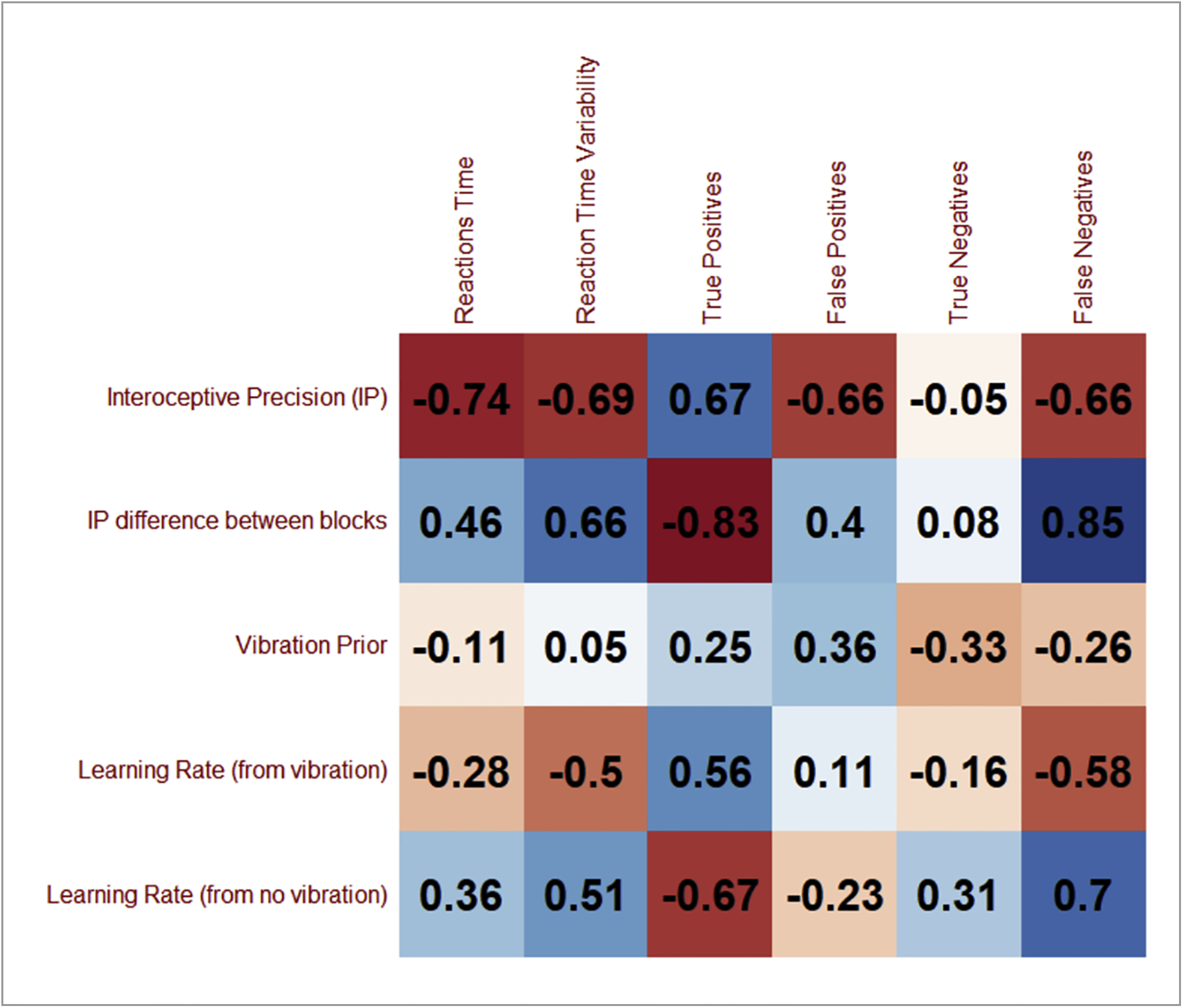
Pearson correlations between (log-transformed) parameter values and task reaction times (delay between vibration onset and button press), variability in reactions times, and behavioral accuracy measures (i.e., true/false positives/negatives). We do not show significance indicators as these were not hypothesis tests, but simply descriptive analyses to inform parameter face validity. For reference, a correlation (absolute value) of r > .31 corresponds to an uncorrected p-value less than .05.

Model parameters did not differ by sex. Those who experienced the enhanced block first showed greater IP_diff (t(35) = 3.10, p = .004), learned more slowly from vibrations (t(36) = 2.16, p = .04), and learned more quickly from the absence of vibrations (t(38) = 3.09, p = .004; see Fig. 4).

Fig. 4.

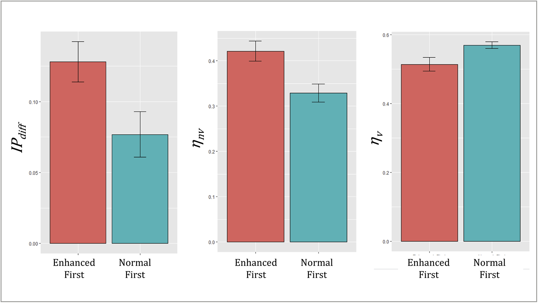
Illustration of order effects between (log-transformed) parameter values (mean ± SE). Those who had the enhanced block first showed a greater decrease in interoceptive precision in the normal block (greater IP_diff), and their prior expectations that a vibration would be felt decreased more quickly (η_nv) and increased more slowly (η_v).

3.3. Relationship to self-report and demographic measures

See Supplementary Table S1 for descriptive statistics for self-report and demographic information, much of which is reproduced from our initial report (Mayeli et al., 2021). Exploratory correlation analyses revealed relationships (p < .05, uncorrected) between model parameters and a number of variables supporting construct validity. For example, both IP and IP_diff were correlated with self-reported detection difficulty and confidence in performance (i.e., as expected, higher IP and a smaller drop in IP between blocks (lower IP_diff) were associated with less perceived difficulty and greater confidence; see Fig. 5 for exact correlation values and associated BFs). Interestingly, greater hunger and thirst at baseline, as well as a more pleasant experience during task performance, were also associated with smaller IP_diff. Priors showed a negative association with BMI and general positive affect ratings on the PANAS. Greater learning rates from vibrations were positively associated with baseline hunger and retrospective confidence in performance, and greater learning rates from the absence of a vibration were associated with a less pleasant task experience. No parameters showed relationships with age or perceived level of focus during the task.

Fig. 5.

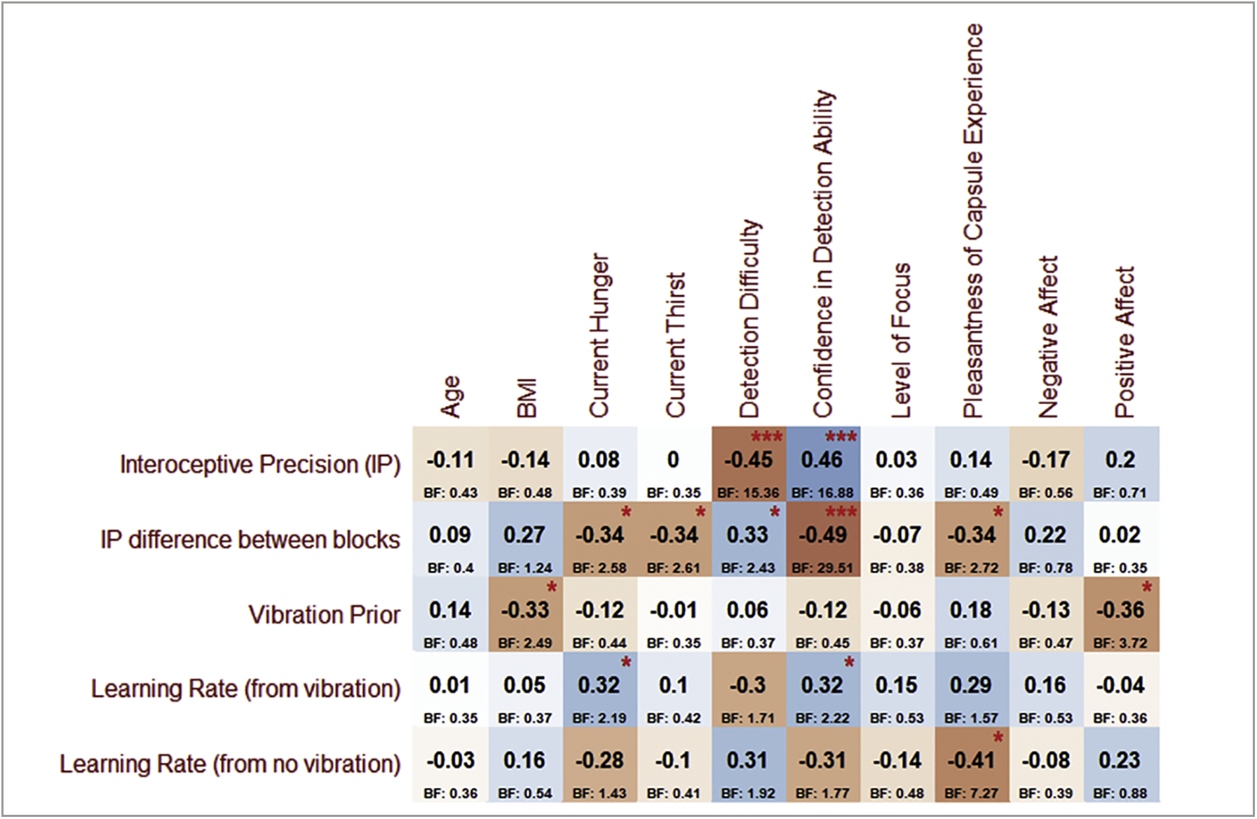
Pearson correlations between (log-transformed) parameter values and individual difference variables of potential interest. For reference, red asterisks indicate uncorrected p-values (*p < .05, ***p < .001). Associated Bayes factors (BF) are listed below each correlation value. BMI = body mass index; Negative and Positive Affect scores are taken from the PANAS (see section on Self-Report Measures for additional information on the scales included in this figure)

Tests of dimensionality in the supplementary canonical correlation analysis associated with exploratory correlations shown in Fig. 5 indicated that the first of five canonical dimensions was statistically significant (canonical correlation = .75, Wilks’ Lambda = .11, p = .045; Roy’s Largest Root = .57, p = .002). The canonical correlations for the second through fifth dimensions were = [0.68, 0.64, 0.43, 0.23]. This supports the predictive validity of these correlational results.

Supplementary Figure S2 shows additional exploratory correlations between parameters and both the ASI and MAIA scales. Overall, there was limited evidence of potential relationships, with the exception of possibly the MAIA ‘body listening’ subscale and learning rates.

3.4. ERP clustering analyses

Fig. 6 illustrates example ERP waveforms evoked by vibrations in both parieto-occipital and frontal electrodes.

For both the early (100–176 ms) and late (300–600 ms) time windows, our clustering analyses yielded the expected optimal 2-cluster solution (silhouette width = .77 and .81, respectively; see Supplementary Figure S3), where one cluster encompassed all parieto-occipital leads and the other encompassed all frontal leads (see Fig. 7). Factor analyses revealed that a single latent factor was sufficient to account for responses across each cluster (χ² values between 213 and 296, all ps < .001). Subsequent PEB analyses therefore focused on these single latent factor scores.

Fig. 7.

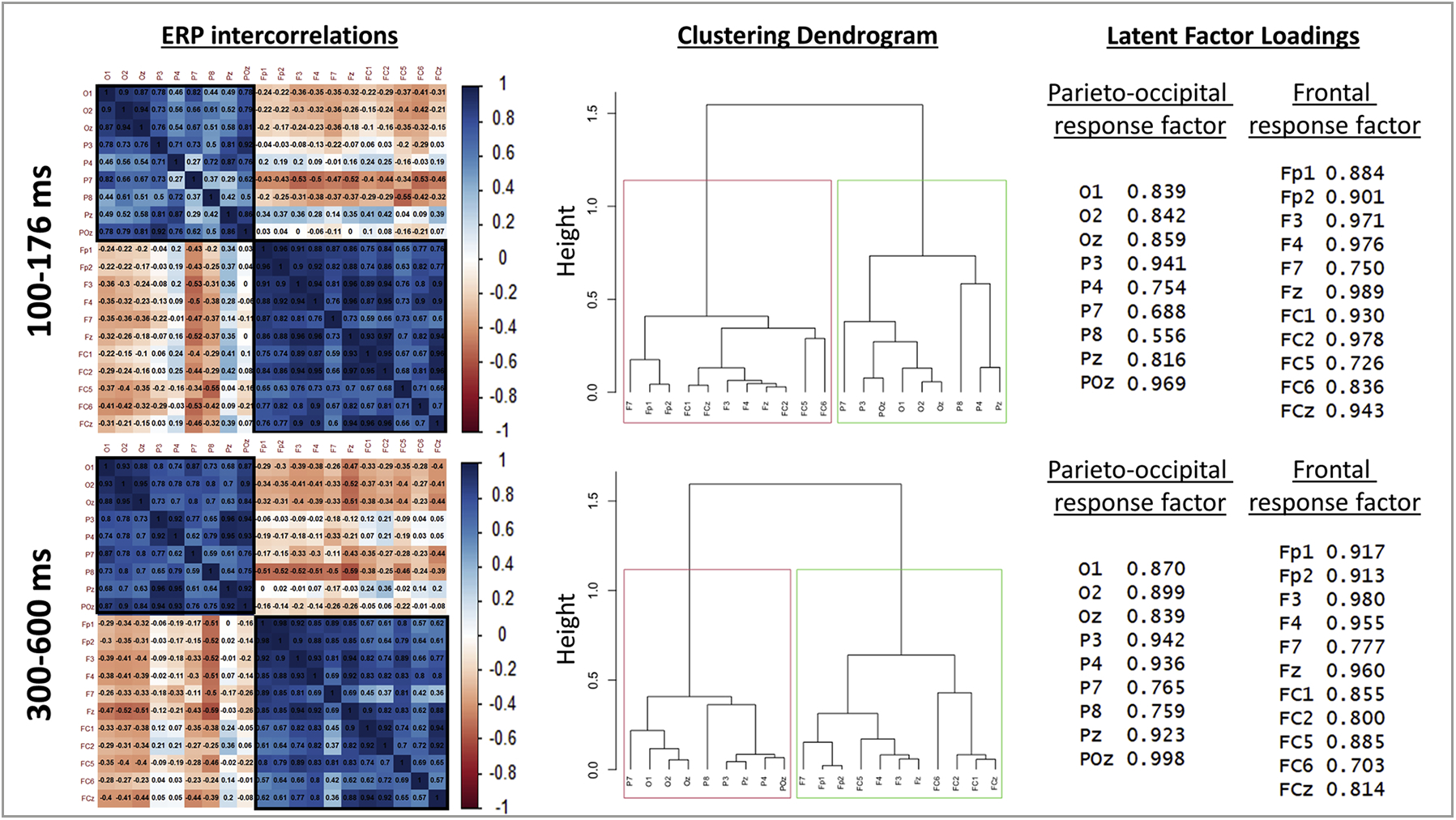
Left: Correlation matrices across all parieto-occipital and frontal electrodes for early (top) and late (bottom) post-vibration ERPs. These plots illustrate the strong and distinct intercorrelations within each respective cluster of electrodes. Middle: Associated dendrograms illustrating that a 2-cluster solution (aggregating parieto-occipital and frontal electrodes, respectively) was optimal, based on average silhouette width. Right: Loadings of each electrode onto the respective latent factors accounting for common activation patterns in each cluster.

3.5. Parieto-occipital ERPs

The winning (reduced) model within PEB analyses testing for relationships between model parameters and the latent parieto-occipital response factor in the early (100–176 ms) time window provided very strong evidence for a positive association with IP (posterior probability [pp] = 1; see Fig. 8) and some evidence for associations with pV (positive relationship; pp = .78) and IP_diff (negative relationship; pp = .70). Fig. 8 also shows subsequent post-hoc correlations illustrating that IP and IP_diff showed consistently positive and negative relationships (respectively) across several parieto-occipital leads. Consistent (but weaker) positive associations were also present with pV across leads. Note here that the differences between PEB results and these zero-order correlations are accounted for by included covariates as well as the way in which PEB considers posterior distributions over parameters (i.e., means and variances) as opposed to simply using the posterior means as point estimates.

Fig. 8.

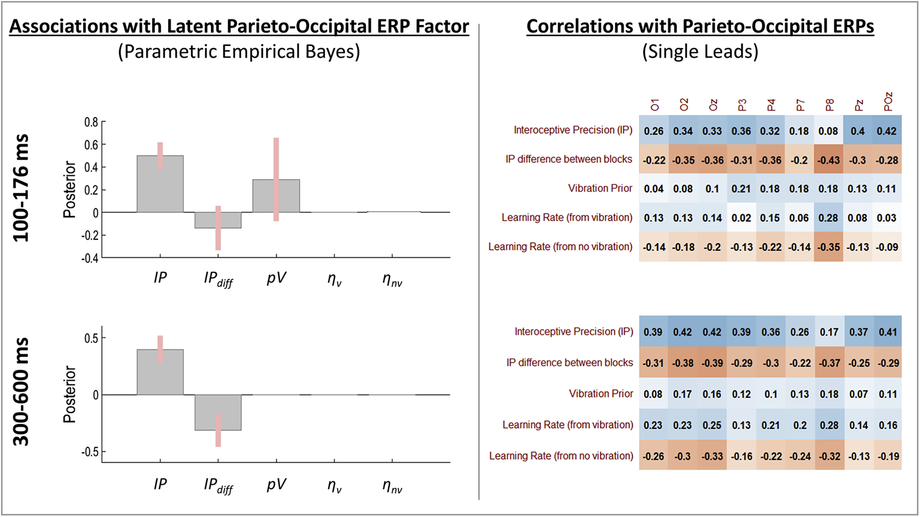
Left: Results of Parametric Empirical Bayes (PEB) analyses assessing evidence for a relationship between the posterior distribution (mean and variance) for individual-level model parameter estimates and the latent factor underlying covariance across the cluster of parieto-occipital ERPs. Group-level posterior means and 95% Bayesian confidence intervals are displayed for each parameter such that the direction (above or below 0) indicates the direction of the relationship (values are in logit space). Right: Subsequent post-hoc Pearson correlations with ERPs from each parieto-occipital lead. These are descriptive and were carried out to further illustrate relationships detected in the PEB analyses. Note that differences between PEB results and these zero-order correlations are accounted for by covariates included in the PEB models as well as by the way in which PEB considers posterior distributions over parameters (i.e., means and variances) as opposed to simply using the posterior means as point estimates. For the interested reader, we note that a correlation value of r = .31 or greater corresponds to an uncorrected significance level of p < .05.

The winning model within PEB analyses testing for relationships between model parameters and the latent parieto-occipital response factor in the later (300–600 ms) time window provided very strong evidence for positive associations with IP (see Fig. 8; pp = 1) and negative associations with IP_diff (pp = .99), consistent with the strong positive and negative relationships (respectively) across the several parieto-occipital leads also shown in Fig. 8.

3.6. Frontal ERPs

The winning model within PEB analyses testing for relationships between model parameters and the latent frontal response factor in the early (100–176 ms) time window provided strong evidence for a positive association with IP (see Fig. 9; pp = .96). As also depicted in Fig. 9, IP showed a consistently positive (but weak) association across several frontal leads. The winning model within PEB analyses testing for relationships between model parameters and the latent frontal response factor in the latter (300–600 ms) time window provided positive evidence for a negative association with pV (see Fig. 9; pp = .89) and strong evidence for a positive association with η_nv (pp = .98). There was also some evidence for a positive association with IP_diff (pp = .78). As shown in Fig. 9, this pattern of relationships was present across several frontal leads.

Fig. 9.

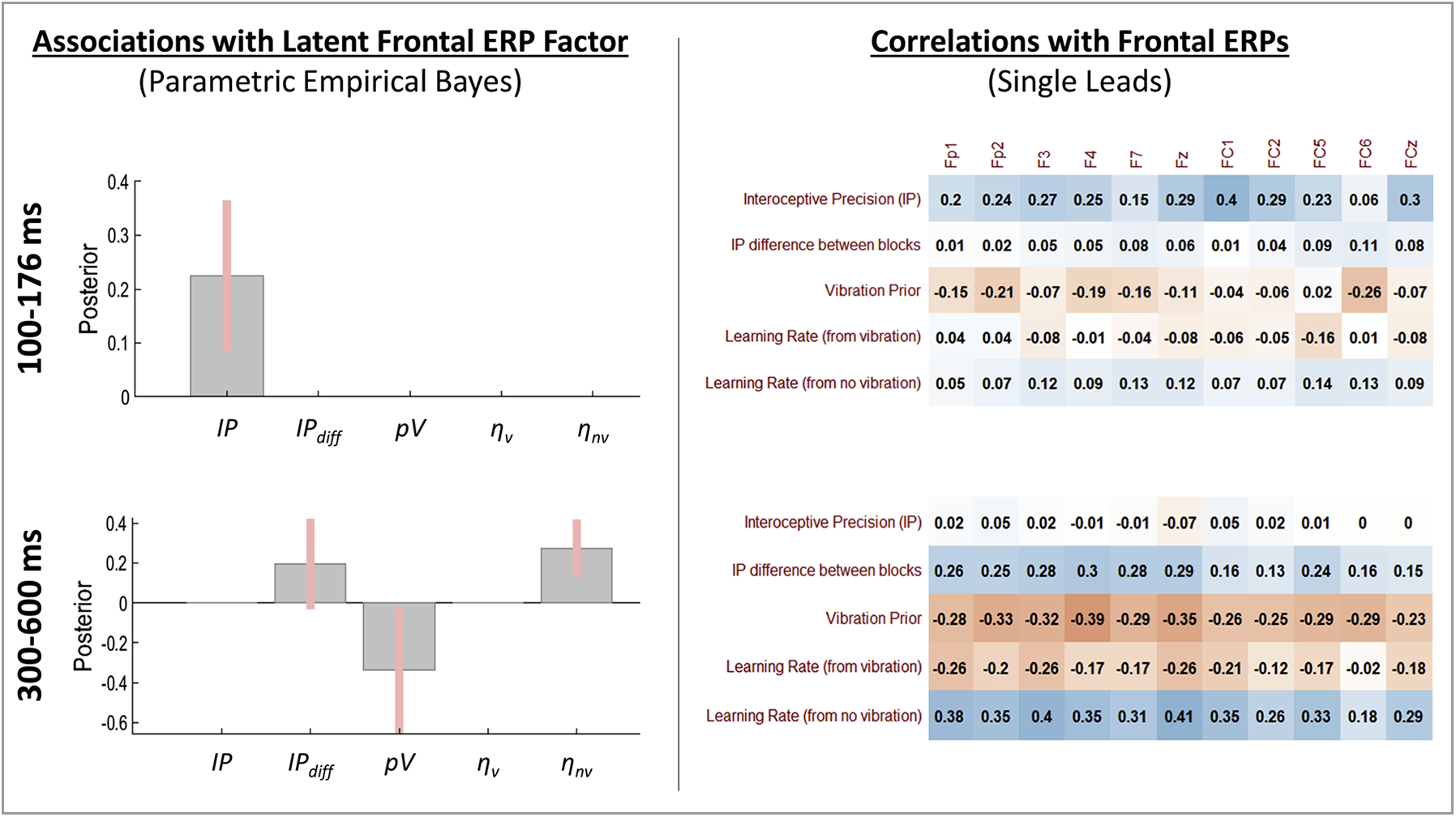
Left: Results of Parametric Empirical Bayes (PEB) analyses assessing evidence for a relationship between the posterior distribution (mean and variance) for individual-level model parameter estimates and the latent factor underlying covariance across the cluster of frontal ERPs. Group-level posterior means and 95% Bayesian confidence intervals are displayed for each parameter such that the direction (above or below 0) indicates the direction of the relationship (values are in logit space). Right: Subsequent post-hoc Pearson correlations with ERPs from each frontal lead. These are descriptive and were carried out to further illustrate relationships detected in the PEB analyses. Note that differences between PEB results and these zero-order correlations are accounted for by covariates included in the PEB models as well as by the way in which PEB considers posterior distributions over parameters (i.e., means and variances) as opposed to simply using the posterior means as point estimates. For the interested reader, we note that a correlation value of r = .31 or greater corresponds to an uncorrected significance level of p < .05.

3.7. Exploratory analyses of peripheral physiology

As we had no specific hypotheses regarding the EGG signal, we ran exploratory correlation analyses between EGG power and model parameters. While no associations were found between EGG and model parameters at baseline or during the enhanced block, there were significant correlations with EGG total power in the normal block for both IP (r(40) = −0.43, p = .006, BF = 9.8) and pV (r(40) = .41, p = .009, BF = 6.8). Subsequent analyses suggested that the relationship with IP was driven by all frequency bands (rs(40) = −0.3 to −.44, ps = .005–.06, BFs = 1.7–12.3), while the relationship with pV was driven primarily by the normogastria frequency band (r(40) = .42, p = .007, BF = 8.8; see Supplementary Figure S4). Skin conductance responses (maximum phasic response values) to vibrations across the task showed a positive association with IP (r(40) = .40, p = .01, BF = 6.7), and heart rate responses to vibrations across the task showed a positive association with η_v (r(40) = .34, p = .01, BF = 2.7). No associations were found with average heart rate. These relationships showed a similar pattern when analyzing the normal and enhanced blocks separately (see Supplementary Figure S4).

3.8. Block order effects

Because our results suggested that block order had an influence on parameter values, we ran supplementary analyses to examine whether the relationships between parameters and ERP results might also show different patterns. Supplementary Figures S5–S6 show correlation matrices examining these relationships for each block order separately. While many relationships were qualitatively similar, some suggestive differences were present (while noting the reduced sample size in each sub-group and resulting reduction in the stability/reliability of these correlations). For example, it was notable in both time windows that pV showed a pattern of positive relationships with parieto-occipital ERPs when the normal block was presented first, while there was a pattern of negative relationships when the enhanced block was presented first (which may have led these effects to cancel out somewhat across all participants). The relationship between frontal ERPs and IP in the early time window also appeared to be driven by individuals who received the normal-strength stimulation block first.

4. Discussion

In this study we demonstrate a novel method for assessing individual differences in gastrointestinal interoception. This method combines 1) a noninvasive mechanosensory paradigm for measuring gut sensations (Mayeli et al., 2021) with 2) a Bayesian computational modelling approach for analyzing task behavior previously developed for studying cardiac interoception (Smith, Kuplicki, Feinstein et al., 2020; Smith, Kuplicki, Teed et al., 2020). However, unlike most cardiac interoception tasks, because the capsule vibration signal strength and timing could be precisely controlled, Bayesian modelling was able to estimate additional parameters when characterizing the belief updating underlying behavior. This included not only sensory precision and prior expectations, but also learning rates and changes in precision with different signal strengths. In other words, our modelling approach could identify individual differences in how prior beliefs evolve over time during the task and how these interact with internal estimates of the reliability of afferent GI signals.

Correlations with model-free measures of task behavior confirmed that model parameters tracked consistent patterns in behavior (e.g., higher precision with higher accuracy, stronger priors with higher numbers of false positives), but that each parameter accounted for different behavioral patterns to different degrees. Several model parameters were also strongly correlated with reaction times in anticipated directions (e.g., higher precision was associated with faster reaction times, suggesting a faster perceptual evidence accumulation rate). Because the model was not fit to reaction times, this provides stronger support for parameter construct validity than the relationships with accuracy. The model was also validated by self-report measures, where higher precision and faster learning rate (from felt vibrations) both correlated with greater self-perceived task performance (i.e., lower perceived difficulty and higher confidence).

Interestingly, those who received the enhanced block first showed a greater decrease in interoceptive precision in the normal block, which could indicate that they came to expect a more precise signal in the enhanced block – thereby reducing confidence when subsequently feeling the weaker signal in the normal block. This dynamic was not facilitated by the reverse ordering, suggesting that providing the enhanced block first may be a more sensitive approach to detecting certain individual differences. Future studies could capitalize on this effect by choosing an ordering most sensitive to individual differences in parameters of greatest interest, similar to the way auditory stimulus ordering has been used to build up prior expectations that promote perceptual illusions or ‘hallucinated stimuli’ in psychosis research (Powers, Mathys, & Corlett, 2017). In our supplementary analyses, for example, there were hints that presenting the enhanced vs. normal block first elicited distinct patterns of relationships between prior expectations and a number of EEG responses (e.g., positive relationships between pV and several parieto-occipital electrodes with normal-first, but negative relationships with enhanced-first).

As an additional validation, we then examined predicted relationships with event-related potentials (ERPs). The neural process theory associated with active inference models (from which our Bayesian model was derived; (Friston, FitzGerald et al., 2016, 2017; Parr & Friston, 2018; Smith, Friston et al., 2021)) postulates that firing rates in specific neuronal populations encode the strength of belief in one perceptual interpretation vs. another (here, the interpretation that a vibration state was or was not present). The rate of change in firing rates (corresponding to rate of change in beliefs or speed of evidence accumulation) should consequently generate stronger ERPs. The neural process theory also postulates that deeper levels in a neural hierarchy provide perceptual processing with prior expectations, and that changes in these expectations (and associated learning rates) operate over slower timescales. This motivated our hypotheses that higher interoceptive precision should correspond to stronger ERPs in perceptual (i.e., parieto-occipital) regions and that stronger prior expectations to feel a vibration (and a slower decay in these expectations; i.e., both promoting less surprise) should dampen ERPs in higher frontal regions. These associations would also be expected within the closely related theory of predictive coding (Bogacz, 2017), which describes perceptual inference as a process of updating beliefs to minimize precision-weighted prediction errors – where higher sensory precision amplifies prediction errors (and therefore ERPs), while stronger (more precise) prior beliefs downweight prediction errors (dampening ERPs). Consistent with our predictions and the hypothesized link between precision, belief updating, and ERPs, the Bayesian analyses and post-hoc correlations confirmed that several parieto-occipital electrodes showed stronger responses to capsule vibrations with higher sensory precision. Further, several frontal electrodes showed dampened responses with more precise prior expectations and in individuals who showed a slower rate of decay in those prior expectations (i.e., slower learning rate from the absence of a vibration). Interestingly, the association between frontal regions and prior expectations and learning rates was only present at the later (300–600 ms) time window – consistent with the idea that learning occurs over slower time scales than perception (Bogacz, 2017; Friston, FitzGerald et al., 2016; Kiebel et al., 2008; Murray et al., 2014). These results each provide additional support for the hypothesis that prior expectations, and their evolution over time, are associated with deeper (frontal) levels in a processing hierarchy. It also provides empirical support for the postulated relationship between belief updating and ERPs in active inference (Friston, Parr et al., 2017; Parr, Markovic, Kiebel, & Friston, 2019; Smith, Friston et al., 2021).

We also explored whether computational model parameters might show relationships with peripheral electrophysiological patterns associated with skin conductance, heart rate, and stomach activity (EGG signal). We found that phasic skin conductance changes (indexing evoked autonomic activity) were positively associated with interoceptive precision, consistent with the notion that signals are more surprising (i.e., they lead to greater belief updating) when they are believed to be precise. We further found that those who learned faster in response to vibrations showed greater heart rate changes in response to each vibration. This latter finding appears consistent with theories of arousal-facilitated learning (e.g., see (Mather, Clewett, Sakaki, & Harley, 2015)), but we stress that these results are preliminary and strong interpretation will not be warranted until they are replicated in future work.

Finally, we found that both prior beliefs and interoceptive precision were associated with EGG signals during periods of normal (but not enhanced) vibration strength. Because the baseline (pre-task) EGG signal was not associated with these parameters, it could be argued that capsule vibration may have influenced stomach activity in a manner that depended on differences in prior beliefs and beliefs about the precision of the afferent signal (i.e., suggesting an effect that could also be perceptually mediated). However, our prior report (Mayeli et al., 2021) found no change in EGG from baseline to normal vibration periods at the group level. With this in mind, our results could suggest that the presence of the afferent signal may have led to increases in EGG power from baseline in those whose vibration percepts were more strongly driven by prior beliefs (i.e., under-constrained by the afferent signal), while greater sensitivity to the afferent signal instead promoted reductions in EGG power from baseline. One possible reason why this relationship may have been absent in the enhanced vibration block is a ceiling effect. Specifically, performance was quite high (and less variable) on average in this block, suggesting that the signal may have been too precise – potentially leading to a reduced sensitivity to detect individual differences that manifest primarily at weaker signal strengths. The precise functional significance and correct causal interpretation of the relationship between EGG and priors/precision is unclear, and we do not interpret it further. However, future studies might examine the degree to which this individual difference indicator could illuminate perceptual processing in specific groups of individuals, such as in clinical populations characterized by faulty inferences about body states and symptoms (Van den Bergh, Witthoft, Petersen, & Brown, 2017). For example, abnormal predictions about body sensations (including bloating, cramping, fullness, or hunger) are considered to play a role in conditions such as eating disorders (Bernardoni et al., 2018; Frank, Collier, Shott, & O’Reilly, 2016; Kaye, Fudge, & Paulus, 2009; Khalsa et al., 2015), somatic symptom disorders (Barsky, Peekna, & Borus, 2001; Flasinski et al., 2020), functional neurological disorders (Drane et al., 2020; Edwards et al., 2012; Espay et al., 2018), and functional bowel disorders (Kwan et al., 2005; Simren et al., 2018; Smith, Gudleski, Lane, & Lackner, 2019; Tillisch & Mayer, 2005).

Here it is also worth considering how our results might build on previous interoception research involving other GI stimulation methods, many of which have focused on the esophagus and colon. For example, one common method for assessing GI interoception is electrical stimulation of the esophagus (Frieling, Enck, & Wienbeck, 1989). Consistent with our computational framework, studies using this approach have found that the amplitude of cortical evoked potentials decreases with an increasing number of stimulations – as would be expected if the brain builds up prior expectations for the presentation of a stimulus over time (Frieling et al., 1989; Frobert et al., 1994; Frobert, Arendt-Nielsen, Bak, Funch-Jensen, & Bagger, 1995; Sollenbohmer, Enck, Haussinger, & Frieling, 1996; Tougas, Hudoba, Fitzpatrick, Hunt, & Upton, 1993). This same dynamic would also be predicted by our model if ERPs were assessed on a vibration-by-vibration basis, which will be an important future direction (for related EEG studies of esophageal stimulation using balloon distention, see (Castell, Wood, Frieling, Wright, & Vieth, 1990; Smout, DeVore, Dalton, & Castell, 1992; Weusten, Franssen, Wieneke, & Smout, 1994)). Another widely used approach has been stimulation of the sigmoid colon, using either electrical- or balloon distension-based stimuli. This approach has previously been used to show how detection of colon stimulation can be dissociated from reportable sensations in common psychophysics and forced-choice paradigms (Holzl, Erasmus, & Moltner, 1996). While not done here, our paradigm could allow the possibility of assessing similar phenomena for stomach sensations (and their neurocomputational basis) by considering vibration periods where individuals do vs. do not report a sensation. These esophageal and colon stimulation studies have implicated somatosensory, insula, and cingulate brain regions consistent with the correlates of our prior expectation and learning rate parameters (for a review, see (Aziz & Thompson, 1998)), while more recent work has also characterized a “gastric network” including posterior parietal regions consistent with correlates of our interoceptive sensory precision parameters (Rebollo, Devauchelle, Beranger, & Tallon-Baudry, 2018). It will be important for future research to further disentangle how computational mechanisms relate to this prior body of work.

Our computational modelling approach to this task is not without limitations. While model parameters were recoverable, and model comparison supported our model as having the most evidence, other generative models might have been considered (e.g., the Hierarchical Gaussian Filter; (Mathys et al., 2014)). Our approach also requires a choice of how to discretize time (e.g., where we here considered each 3-second period as a “trial”). Our choice was based on the length of vibration intervals, but other discretization schemes might have been used. The task is also novel, with a number of limitations in interpretability described in more detail in our prior report (e.g., the specific molecular signal transduction mechanisms and afferent neuronal pathways by which the vibration signal reaches the brain are unclear; (Mayeli et al., 2021)). Our sample size was also relatively small by modern standards and provided limited power to detect significant relationships in our exploratory correlation analyses (e.g., in Fig. 5). The exploratory nature of several of our correlational analyses also entails that – beyond their use as validating the novel method we have described – they should be considered primarily as hypothesis generating. Future studies with larger samples and strong a priori hypotheses will therefore be necessary to confirm the patterns of relationships we observed. Finally, our selection of ERP time windows was based mainly on initial visible inspection of the ERP waveform (and based on differences between ERPs evoked by the normal vs. enhanced conditions described in our prior report; see (Mayeli et al., 2021)). Future studies might examine other time windows and could benefit from more sophisticated means of time window selection.

With these limitations in mind, our paradigm also has important strengths that merit its use in further work. Namely, unlike traditional cardiac perception tasks, the timing and strength of the interoceptive signal can be precisely controlled, without resorting to invasive means. The mechanosensory means of stimulation taps into a clinically significant interoceptive modality (‘gut feelings’ within the GI system) that has been understudied in the psychological literature due to the inaccessibility of the body’s interior. This method allows for fast, repeatable GI stimulations (unlike other measures of GI interoception; e.g., water loading (van Dyck et al., 2016)) and consequently affords more sophisticated analyses. Namely, it lends itself to computational modelling approaches such as those used here that treat perception as Bayesian inference and that afford estimation of individual differences in a number of information processing mechanisms (i.e., here, five distinct computational parameters). However, it should be acknowledged that, while offering these methodological advantages, our mechanosensory paradigm was not designed to simulate naturalistic states of the GI system. It remains an open question whether individual differences in the ability to detect vibratory stimulation will generalize to differences in the perception of naturally occurring GI states.

In conclusion, this foundational work establishes the predictive and face validity of applying a novel computational modelling approach to a recent interoceptive paradigm for understanding gut sensation, which affords a quantitative phenotyping of individual participants in terms of their sensitivity to – and subsequent inferences about – interoceptive states. By using Bayesian belief updating to explain both behavioral and physiological responses, we were able to quantify the way that participants infer and learn about their gut feelings. This provides a unique opportunity to evaluate how the human brain infers gastrointestinal states, paving the way for future studies assessing the predictive value of the individual differences revealed by our approach in clinical populations, especially those in which gastrointestinal symptoms are prominent.

References

- Adams R, Perrinet L, & Friston KJ (2012). Smooth pursuit and visual occlusion: Active inference and oculomotor control in schizophrenia. PloS One, 7, e47502. 10.1371/journal.pone.0047502 [DOI] [PMC free article] [PubMed] [Google Scholar]
- Adams R, Shipp S, & Friston K (2013). Predictions not commands: Active inference in the motor system. Brain Structure & Function, 218, 611–643. 10.1007/s00429-012-0475-5 [DOI] [PMC free article] [PubMed] [Google Scholar]
- Ainley V, Tsakiris M, Pollatos O, Schulz A, & Herbert BM (2020). Comment on “Zamariola et al. (2018), Interoceptive accuracy scores are problematic: Evidence from simple bivariate correlations”-the empirical data base, the conceptual reasoning and the analysis behind this statement are misconceived and do not support the authors’ conclusions. Biological Psychology, 152, 107870. 10.1016/j.biopsycho.2020.107870 [DOI] [PubMed] [Google Scholar]
- Allen M, Levy A, Parr T, & Friston KJ (2019). In the body’s eye: The computational anatomy of interoceptive inference. bioRxiv, 603928. 10.1101/603928 [DOI] [PMC free article] [PubMed] [Google Scholar]
- Aziz Q, & Thompson DG (1998). Brain-gut axis in health and disease. Gastroenterology, 114(3), 559–578. 10.1016/s0016-5085(98)70540-2 [DOI] [PubMed] [Google Scholar]
- Bach DR (2014). A head-to-head comparison of SCRalyze and Ledalab, two model-based methods for skin conductance analysis. Biological Psychology, 103, 63–68. 10.1016/j.biopsycho.2014.08.006 [DOI] [PMC free article] [PubMed] [Google Scholar]
- Barrett L, & Simmons W (2015). Interoceptive predictions in the brain. Nature reviews. Neuroscience, 16, 419–429. 10.1038/nrn3950 [DOI] [PMC free article] [PubMed] [Google Scholar]
- Barsky AJ, Peekna HM, & Borus JF (2001). Somatic symptom reporting in women and men. Journal of General Internal Medicine, 16(4), 266–275. Retrieved from https://www.ncbi.nlm.nih.gov/pubmed/11318929. [DOI] [PMC free article] [PubMed] [Google Scholar]
- Bastos A, Usrey W, Adams R, Mangun G, Fries P, & Friston K (2012). Canonical microcircuits for predictive coding. Neuron, 76, 695–711. 10.1016/j.neuron.2012.10.038 [DOI] [PMC free article] [PubMed] [Google Scholar]
- Bell AJ, & Sejnowski TJ (1995). An information-maximization approach to blind separation and blind deconvolution. Neural Computation, 7(6), 1129–1159. [DOI] [PubMed] [Google Scholar]
- Benini L, Todesco T, Dalle Grave R, Deiorio F, Salandini L, & Vantini I (2004). Gastric emptying in patients with restricting and binge/purging subtypes of anorexia nervosa. The American Journal of Gastroenterology, 99(8), 1448–1454. 10.1111/j.1572-0241.2004.30246.x [DOI] [PubMed] [Google Scholar]
- Bernardoni F, Geisler D, King JA, Javadi AH, Ritschel F, Murr J, … Ehrlich S (2018). Altered medial frontal feedback learning signals in anorexia nervosa. Biological Psychiatry, 83(3), 235–243. 10.1016/j.biopsych.2017.07.024 [DOI] [PubMed] [Google Scholar]
- Berntson GG, & Khalsa SS (2021). Neural circuits of interoception. Trends in Neurosciences, 44(1), 17–28. 10.1016/j.tins.2020.09.011 [DOI] [PMC free article] [PubMed] [Google Scholar]
- Bluemel S, Menne D, Milos G, Goetze O, Fried M, Schwizer W, … Steingoetter A (2017). Relationship of body weight with gastrointestinal motor and sensory function: Studies in anorexia nervosa and obesity. BMC Gastroenterology, 17(1), 4. 10.1186/s12876-016-0560-y [DOI] [PMC free article] [PubMed] [Google Scholar]
- Bogacz R (2017). A tutorial on the free-energy framework for modelling perception and learning. Journal of Mathematical Psychology, 76, 198–211. 10.1016/j.jmp.2015.11.003 [DOI] [PMC free article] [PubMed] [Google Scholar]
- Bonaz B, Lane RD, Oshinsky ML, Kenny PJ, Sinha R, Mayer EA, … Critchley HD (2021). Diseases, disorders, and comorbidities of interoception. Trends in Neurosciences, 44(1), 39–51. 10.1016/j.tins.2020.09.009 [DOI] [PubMed] [Google Scholar]
- Browning M, Behrens TE, Jocham G, O’Reilly JX, & Bishop SJ (2015). Anxious individuals have difficulty learning the causal statistics of aversive environments. Nature Neuroscience, 18(4), 590–596. 10.1038/nn.3961 [DOI] [PMC free article] [PubMed] [Google Scholar]
- Cameron OG, & Minoshima S (2002). Regional brain activation due to pharmacologically induced adrenergic interoceptive stimulation in humans. Psychosomatic Medicine, 64(6), 851–861. 10.1097/01.psy.0000038939.33335.32 [DOI] [PubMed] [Google Scholar]
- Castell DO, Wood JD, Frieling T, Wright FS, & Vieth RF (1990). Cerebral electrical potentials evoked by balloon distention of the human esophagus. Gastroenterology, 98(3), 662–666. 10.1016/0016-5085(90)90286-a [DOI] [PubMed] [Google Scholar]
- Chen C, Takahashi T, Nakagawa S, Inoue T, & Kusumi I (2015). Reinforcement learning in depression: A review of computational research. Neuroscience and Biobehavioral Reviews, 55, 247–267. 10.1016/j.neubiorev.2015.05.005 [DOI] [PubMed] [Google Scholar]
- Chen WG, Schloesser D, Arensdorf AM, Simmons JM, Cui C, Valentino R, … Langevin HM (2021). The emerging science of interoception: Sensing, integrating, interpreting, and regulating signals within the self. Trends in Neurosciences, 44(1), 3–16. 10.1016/j.tins.2020.10.007 [DOI] [PMC free article] [PubMed] [Google Scholar]
- Clark JE, Watson S, & Friston KJ (2018). What is mood? A computational perspective. Psychological Medicine, 1–8. 10.1017/S0033291718000430 [DOI] [PMC free article] [PubMed] [Google Scholar]
- Corneille O, Desmedt O, Zamariola G, Luminet O, & Maurage P (2020). A heartfelt response to Zimprich et al. (2020), and Ainley et al. (2020)’s commentaries: Acknowledging issues with the HCT would benefit interoception research. Biological Psychology, 152, 107869. 10.1016/j.biopsycho.2020.107869 [DOI] [PubMed] [Google Scholar]
- Da Costa L, Parr T, Sajid N, Veselic S, Neacsu V, & Friston KJ (2020). Active inference on discrete state-spaces: A synthesis. Journal of Mathematical Psychology, 99, Article 102447. [DOI] [PMC free article] [PubMed] [Google Scholar]
- Desmedt O, Luminet O, & Corneille O (2018). The heartbeat counting task largely involves non-interoceptive processes: Evidence from both the original and an adapted counting task. Biological Psychology, 138, 185–188. 10.1016/j.biopsycho.2018.09.004 [DOI] [PubMed] [Google Scholar]
- Diamanti A, Bracci F, Gambarara M, Ciofetta GC, Sabbi T, Ponticelli A, … Castro M (2003). Gastric electric activity assessed by electrogastrography and gastric emptying scintigraphy in adolescents with eating disorders. Journal of Pediatric Gastroenterology and Nutrition, 37(1), 35–41. Retrieved from https://www.ncbi.nlm.nih.gov/pubmed/12827003. [DOI] [PubMed] [Google Scholar]
- Dirgenali F, Kara S, & Okkesim Ş (2006). Estimation of wavelet and short-time Fourier transform sonograms of normal and diabetic subjects’ electrogastrogram. Computers in Biology and Medicine, 36(12), 1289–1302. [DOI] [PubMed] [Google Scholar]
- Drane DL, Fani N, Hallett M, Khalsa SS, Perez DL, & Roberts NA (2020). A framework for understanding the pathophysiology of functional neurological disorder. CNS Spectrums, 1–7. 10.1017/S1092852920001789 [DOI] [PMC free article] [PubMed] [Google Scholar]
- Edwards M, Adams R, Brown H, Pareés I, & Friston K (2012). A Bayesian account of’ hysteria’. Brain, 135, 3495–3512. 10.1093/brain/aws129 [DOI] [PMC free article] [PubMed] [Google Scholar]
- Espay AJ, Aybek S, Carson A, Edwards MJ, Goldstein LH, Hallett M, … Morgante F (2018). Current concepts in diagnosis and treatment of functional neurological disorders. JAMA Neurology, 75(9), 1132–1141. 10.1001/jamaneurol.2018.1264 [DOI] [PMC free article] [PubMed] [Google Scholar]
- Flasinski T, Dierolf AM, Rost S, Lutz APC, Voderholzer U, Koch S, … Schulz A (2020). Altered interoceptive awareness in high habitual symptom reporters and patients with somatoform disorders. Frontiers in Psychology, 11, 1859. 10.3389/fpsyg.2020.01859 [DOI] [PMC free article] [PubMed] [Google Scholar]
- Frank GK, Collier S, Shott ME, & O’Reilly RC (2016). Prediction error and somatosensory insula activation in women recovered from anorexia nervosa. Journal of Psychiatry & Neuroscience : JPN, 41(5), 304–311. 10.1503/jpn.150103 [DOI] [PMC free article] [PubMed] [Google Scholar]
- Frieling T, Enck P, & Wienbeck M (1989). Cerebral responses evoked by electrical stimulation of the esophagus in normal subjects. Gastroenterology, 97(2), 475–478. 10.1016/0016-5085(89)90087-5 [DOI] [PubMed] [Google Scholar]
- Friston KJ (2005). A theory of cortical responses. Philosophical Transactions of the Royal Society of London Series B, Biological Sciences, 360, 815–836. 10.1098/rstb.2005.1622 [DOI] [PMC free article] [PubMed] [Google Scholar]
- Friston KJ, Mattout J, Trujillo-Barreto N, Ashburner J, & Penny W (2007). Variational free energy and the Laplace approximation. Neuroimage, 34, 220–234. 10.1016/J.NEUROIMAGE.2006.08.035 [DOI] [PubMed] [Google Scholar]
- Friston KJ, Stephan K, Montague R, & Dolan R (2014). Computational psychiatry: The brain as a phantastic organ. The Lancet Psychiatry, 1, 148–158. 10.1016/S2215-0366(14)70275-5 [DOI] [PubMed] [Google Scholar]
- Friston KJ, FitzGerald T, Rigoli F, Schwartenbeck P, O’Doherty J, & Pezzulo G (2016). Active inference and learning. Neuroscience and Biobehavioral Reviews, 68, 862–879. 10.1016/j.neubiorev.2016.06.022 [DOI] [PMC free article] [PubMed] [Google Scholar]
- Friston KJ, FitzGerald T, Rigoli F, Schwartenbeck P, & Pezzulo G (2017). Active inference: A process theory. Neural Computation, 29, 1–49. 10.1162/NECO_a_00912 [DOI] [PubMed] [Google Scholar]
- Friston KJ, Lin M, Frith C, Pezzulo G, Hobson J, & Ondobaka S (2017). Active inference, curiosity and insight. Neural Computation, 29, 2633–2683. 10.1162/neco_a_00999 [DOI] [PubMed] [Google Scholar]
- Friston KJ, Litvak V, Oswal A, Razi A, Stephan KE, van Wijk BCM, … Zeidman P (2016). Bayesian model reduction and empirical Bayes for group (DCM) studies. Neuroimage, 128, 413–431. 10.1016/J.NEUROIMAGE.2015.11.015 [DOI] [PMC free article] [PubMed] [Google Scholar]
- Friston KJ, Parr T, & de Vries B (2017). The graphical brain: Belief propagation and active inference. Network Neuroscience, 1, 381–414. 10.1162/NETN_a_00018 [DOI] [PMC free article] [PubMed] [Google Scholar]
- Frobert O, Arendt-Nielsen L, Bak P, Andersen OK, Funch-Jensen P, & Bagger JP (1994). Electric stimulation of the esophageal mucosa. Perception and brain-evoked potentials. Scandinavian Journal of Gastroenterology, 29(9), 776–781. 10.3109/00365529409092509 [DOI] [PubMed] [Google Scholar]
- Frobert O, Arendt-Nielsen L, Bak P, Funch-Jensen P, & Bagger JP (1995). Oesophageal sensation assessed by electrical stimuli and brain evoked potentials–a new model for visceral nociception. Gut, 37(5), 603–609. 10.1136/gut.37.5.603 [DOI] [PMC free article] [PubMed] [Google Scholar]
- Harrison OK, Nanz L, Marino S, Lüchinger R, Hennel F, Hess AJ, Fraessle S, Iglesias S, Vinckier F, Petzschner F, Harrison SJ, & Stephan KE (2021). Interoception of breathing and its relationship with anxiety. bioRxiv. 10.1101/2021.03.24.436881 [DOI] [PMC free article] [PubMed] [Google Scholar]
- Hesp C, Smith R, Allen M, Friston KJ, & Ramstead MJD (2020). Deeply felt affect: The emergence of Valence in deep active inference. Neural Computation, 1–49. 10.1162/neco_a_01341 [DOI] [PMC free article] [PubMed] [Google Scholar]
- Holzl R, Erasmus LP, & Moltner A (1996). Detection, discrimination and sensation of visceral stimuli. Biological Psychology, 42(1–2), 199–214. 10.1016/0301-0511(95)05155-4 [DOI] [PubMed] [Google Scholar]
- Huang H, Thompson W, & Paulus MP (2017). Computational dysfunctions in anxiety: Failure to differentiate signal from noise. Biological Psychiatry, 82(6), 440–446. [DOI] [PMC free article] [PubMed] [Google Scholar]
- Huys Q, Maia T, & Frank M (2016). Computational psychiatry as a bridge from neuroscience to clinical applications. Nature Neuroscience, 19, 404–413. 10.1038/nn.4238 [DOI] [PMC free article] [PubMed] [Google Scholar]
- Kaye WH, Fudge JL, & Paulus M (2009). New insights into symptoms and neurocircuit function of anorexia nervosa. Nature Reviews Neuroscience, 10(8), 573–584. 10.1038/nrn2682 [DOI] [PubMed] [Google Scholar]
- Khalsa SS, & Lapidus RC (2016). Can Interoception Improve the Pragmatic Search for Biomarkers in Psychiatry? Frontiers in Psychiatry, 7, 121. 10.3389/fpsyt.2016.00121 [DOI] [PMC free article] [PubMed] [Google Scholar]
- Khalsa SS, Adolphs R, Cameron OG, Critchley HD, Davenport PW, Feinstein JS, … Interoception Summit, p. (2018). Interoception and mental health: A roadmap. Biological Psychiatry : Cognitive Neuroscience and Neuroimaging, 3(6), 501–513. 10.1016/j.bpsc.2017.12.004 [DOI] [PMC free article] [PubMed] [Google Scholar]
- Khalsa SS, Craske MG, Li W, Vangala S, Strober M, & Feusner JD (2015). Altered interoceptive awareness in anorexia nervosa: Effects of meal anticipation, consumption and bodily arousal. The International Journal of Eating Disorders, 48(7), 889–897. [DOI] [PMC free article] [PubMed] [Google Scholar]
- Khalsa SS, Rudrauf D, Sandesara C, Olshansky B, & Tranel D (2009). Bolus isoproterenol infusions provide a reliable method for assessing interoceptive awareness. International Journal of Psychophysiology : Official Journal of the International Organization of Psychophysiology, 72(1), 34–45. 10.1016/j.ijpsycho.2008.08.010 [DOI] [PMC free article] [PubMed] [Google Scholar]
- Kiebel S, Daunizeau J, & Friston K (2008). A hierarchy of time-scales and the brain. PLoS Computational Biology, 4, e1000209. 10.1371/journal.pcbi.1000209 [DOI] [PMC free article] [PubMed] [Google Scholar]
- Kwan CL, Diamant NE, Pope G, Mikula K, Mikulis DJ, & Davis KD (2005). Abnormal forebrain activity in functional bowel disorder patients with chronic pain. Neurology, 65(8), 1268–1277. 10.1212/01.wnl.0000180971.95473.cc [DOI] [PubMed] [Google Scholar]
- Lee MD, & Wagenmakers EJ (2014). Bayesian cognitive modeling: A practical course. Cambridge university press. [Google Scholar]
- Mather M, Clewett D, Sakaki M, & Harley C (2015). Norepinephrine ignites local hot spots of neuronal excitation: How arousal amplifies selectivity in perception and memory. The Behavioral and Brain Sciences, 1–100. 10.1017/S0140525X15000667 [DOI] [PMC free article] [PubMed] [Google Scholar]
- Mathys CD, Lomakina EI, Daunizeau J, Iglesias S, Brodersen KH, Friston KJ, … Stephan KE (2014). Uncertainty in perception and the hierarchical gaussian filter. Frontiers in Human Neuroscience, 8, 825. 10.3389/fnhum.2014.00825 [DOI] [PMC free article] [PubMed] [Google Scholar]
- Mayeli A, Al Zoubi O, White EJ, Chappelle S, Kuplicki R, Smith R, … Khalsa SS (2021). Neural indicators of human gut feelings. bioRxiv. 10.1101/2021.02.11.430867, 2021.2002.2011.430867. [DOI] [Google Scholar]
- Mayeli A, Henry K, Wong CK, Zoubi OA, White EJ, Luo Q, … Investigators T (2019). Automated pipeline for EEG artifact reduction (APPEAR) recorded during fMRI. arXiv, 1912.05507. [DOI] [PMC free article] [PubMed] [Google Scholar]
- Mayeli A, Zotev V, Refai H, & Bodurka J (2016). Real-time EEG artifact correction during fMRI using ICA. Journal of Neuroscience Methods, 274, 27–37. [DOI] [PubMed] [Google Scholar]
- Mehling WE, Price C, Daubenmier JJ, Acree M, Bartmess E, & Stewart A (2012). The multidimensional assessment of interoceptive awareness (MAIA). PloS One, 7(11), e48230. 10.1371/journal.pone.0048230 [DOI] [PMC free article] [PubMed] [Google Scholar]
- Montague P, Dolan R, Friston K, & Dayan P (2012). Computational psychiatry. Trends in Cognitive Sciences, 16, 72–80. 10.1016/j.tics.2011.11.018 [DOI] [PMC free article] [PubMed] [Google Scholar]
- Morey RD, & Rouder JN (2015). BayesFactor (Version 0.9.10–12)[Computer software]
- Moutoussis M, Shahar N, Hauser T, & Dolan R (2017). Computation in psychotherapy, or how computational psychiatry can aid learning-based psychological therapies. Computational Psychiatry, 1–21. 10.1162/CPSY_a_00014 [DOI] [PMC free article] [PubMed] [Google Scholar]
- Murphy J, Millgate E, Geary H, Ichijo E, Coll MP, Brewer R, … Bird G (2018). Knowledge of resting heart rate mediates the relationship between intelligence and the heartbeat counting task. Biological Psychology, 133, 1–3. 10.1016/j.biopsycho.2018.01.012 [DOI] [PubMed] [Google Scholar]
- Murray J, Bernacchia A, Freedman D, Romo R, Wallis J, Cai X, … Wang X-J (2014). A hierarchy of intrinsic timescales across primate cortex. Nature Neuroscience, 17, 1661–1663. 10.1038/nn.3862 [DOI] [PMC free article] [PubMed] [Google Scholar]
- Nelson A, Camilleri M, Acosta A, Boldingh A, Busciglio I, … Zinsmeister AR (2017). A single-center, prospective, double-blind, sham-controlled, randomized study of the effect of a vibrating capsule on colonic transit in patients with chronic constipation. Neurogastroenterology and Motility : the Official Journal of the European Gastrointestinal Motility Society, 29(7). 10.1111/nmo.13034 [DOI] [PubMed] [Google Scholar]
- Oostenveld R, Fries P, Maris E, & Schoffelen J-M (2011). FieldTrip: Open source software for advanced analysis of MEG, EEG, and invasive electrophysiological data. Computational Intelligence and Neuroscience, 2011. [DOI] [PMC free article] [PubMed] [Google Scholar]
- Owens AP, Allen M, Ondobaka S, & Friston KJ (2018). Interoceptive inference: From computational neuroscience to clinic. Neuroscience and Biobehavioral Reviews, 90, 174–183. 10.1016/j.neubiorev.2018.04.017 [DOI] [PubMed] [Google Scholar]
- Owens AP, Friston KJ, Low D, Mathias C, & Critchley H (2018). Investigating the relationship between cardiac interoception and autonomic cardiac control using a predictive coding framework. Autonomic Neuroscience, 210, 65–71. 10.1016/J.AUTNEU.2018.01.001 [DOI] [PubMed] [Google Scholar]
- Parr T, & Friston KJ (2017). Working memory, attention, and salience in active inference. Scientific Reports, 7, 14678. 10.1038/s41598-017-15249-0 [DOI] [PMC free article] [PubMed] [Google Scholar]
- Parr T, & Friston KJ (2018). The anatomy of inference: Generative models and brain structure. Frontiers in Computational Neuroscience, 12, 90. 10.3389/fncom.2018.00090 [DOI] [PMC free article] [PubMed] [Google Scholar]
- Parr T, Markovic D, Kiebel S, & Friston KJ (2019). Neuronal message passing using Mean-field, Bethe, and Marginal approximations. Scientific Reports, 9, 1889. 10.1038/s41598-018-38246-3 [DOI] [PMC free article] [PubMed] [Google Scholar]
- Paulus MP, Feinstein JS, & Khalsa SS (2019). An active inference approach to interoceptive psychopathology. Annual Review of Clinical Psychology, 15, 97–122. 10.1146/annurev-clinpsy-050718-095617 [DOI] [PMC free article] [PubMed] [Google Scholar]
- Petzschner FH, Garfinkel SN, Paulus MP, Koch C, & Khalsa SS (2021). Computational models of interoception and body regulation. Trends in Neurosciences, 44(1), 63–76. 10.1016/j.tins.2020.09.012 [DOI] [PMC free article] [PubMed] [Google Scholar]
- Petzschner FH, Weber L, Gard T, & Stephan K (2017). Computational psychosomatics and computational psychiatry: Toward a joint framework for differential diagnosis. Biological Psychiatry, 82, 421–430. 10.1016/j.biopsych.2017.05.012 [DOI] [PubMed] [Google Scholar]
- Petzschner FH, Weber LA, Wellstein KV, Paolini G, Do CT, & Stephan KE (2019). Focus of attention modulates the heartbeat evoked potential. Neuroimage, 186, 595–606. 10.1016/j.neuroimage.2018.11.037 [DOI] [PubMed] [Google Scholar]
- Phillips GC, Jones GE, Rieger EJ, & Snell JB (1999). Effects of the presentation of false heart-rate feedback on the performance of two common heartbeat-detection tasks. Psychophysiology, 36(4), 504–510. Retrieved from https://www.ncbi.nlm.nih.gov/pubmed/10432800. [DOI] [PubMed] [Google Scholar]
- Powers AR, Mathys C, & Corlett PR (2017). Pavlovian conditioning-induced hallucinations result from overweighting of perceptual priors. Science, 357(6351), 596–600. 10.1126/science.aan3458 [DOI] [PMC free article] [PubMed] [Google Scholar]
- Quigley KS, Kanoski S, Grill WM, Barrett LF, & Tsakiris M (2021). Functions of interoception: From energy regulation to experience of the self. Trends in Neurosciences, 44(1), 29–38. 10.1016/j.tins.2020.09.008 [DOI] [PMC free article] [PubMed] [Google Scholar]
- Rao SSC, Lembo A, Chey WD, Friedenberg K, & Quigley EMM (2020). Effects of the vibrating capsule on colonic circadian rhythm and bowel symptoms in chronic idiopathic constipation. Neurogastroenterology and Motility : the Official Journal of the European Gastrointestinal Motility Society, e13890. 10.1111/nmo.13890 [DOI] [PMC free article] [PubMed] [Google Scholar]
- Rebollo I, Devauchelle AD, Beranger B, & Tallon-Baudry C (2018). Stomach-brain synchrony reveals a novel, delayed-connectivity resting-state network in humans. Elife, 7. 10.7554/eLife.33321 [DOI] [PMC free article] [PubMed] [Google Scholar]
- Rigoux L, Stephan KE, Friston KJ, & Daunizeau J (2014). Bayesian model selection for group studies - revisited. Neuroimage, 84, 971–985. 10.1016/j.neuroimage.2013.08.065 [DOI] [PubMed] [Google Scholar]
- Ring C, & Brener J (2018). Heartbeat counting is unrelated to heartbeat detection: A comparison of methods to quantify interoception. Psychophysiology, 55(9), e13084. 10.1111/psyp.13084 [DOI] [PubMed] [Google Scholar]
- Ring C, Brener J, Knapp K, & Mailloux J (2015). Effects of heartbeat feedback on beliefs about heart rate and heartbeat counting: A cautionary tale about interoceptive awareness. Biological Psychology, 104, 193–198. 10.1016/j.biopsycho.2014.12.010 [DOI] [PubMed] [Google Scholar]
- Ron Y, Halpern Z, Safadi R, Dickman R, Dekel R, & Sperber AD (2015). Safety and efficacy of the vibrating capsule, an innovative non-pharmacological treatment modality for chronic constipation. Neurogastroenterology and Motility : the Official Journal of the European Gastrointestinal Motility Society, 27(1), 99–104. 10.1111/nmo.12485 [DOI] [PubMed] [Google Scholar]
- Rouder JN, Morey RD, Speckman PL, & Province JM (2012). Default bayes factors for ANOVA designs. Journal of Mathematical Psychology, 56, 356–374. [Google Scholar]
- Sandin B, Chorot P, & McNally RJ (2001). Anxiety sensitivity index: Normative data and its differentiation from trait anxiety. Behaviour Research and Therapy, 39(2), 213–219. Retrieved from https://www.ncbi.nlm.nih.gov/pubmed/11153974. [DOI] [PubMed] [Google Scholar]
- Schwartenbeck P, & Friston KJ (2016). Computational phenotyping in psychiatry: A worked example. eneuro, 3. 10.1523/ENEURO.0049-16.2016.ENEURO.0049-0016.2016. [DOI] [PMC free article] [PubMed] [Google Scholar]
- Seth A (2013). Interoceptive inference, emotion, and the embodied self. Trends in Cognitive Sciences, 17, 565–573. 10.1016/j.tics.2013.09.007 [DOI] [PubMed] [Google Scholar]
- Seth A, & Critchley H (2013). Extending predictive processing to the body: Emotion as interoceptive inference. The Behavioral and Brain Sciences, 36, 47–48. 10.1017/S0140525X12002270 [DOI] [PubMed] [Google Scholar]
- Sharp PB, & Eldar E (2019). Computational models of anxiety: Nascent efforts and future directions. Current Directions in Psychological Science, 28(2), 170–176. [Google Scholar]
- Sheehan D,V, Lecrubier Y, Sheehan K,H, Amorim P, … Dunbar GC (1998). The Mini-International Neuropsychiatric Interview (MINI): The development and validation of a structured diagnostic psychiatric interview for DSM-IV and ICD-10. The Journal of Clinical Psychiatry. [PubMed] [Google Scholar]
- Simren M, Tornblom H, Palsson OS, van Tilburg MAL, Van Oudenhove L, Tack J, … Whitehead WE (2018). Visceral hypersensitivity is associated with GI symptom severity in functional GI disorders: Consistent findings from five different patient cohorts. Gut, 67(2), 255–262. 10.1136/gutjnl-2016-312361 [DOI] [PubMed] [Google Scholar]
- Smith R, Thayer JF, Khalsa SS, & Lane RD (2017). The hierarchical basis of neurovisceral integration. Neuroscience and Biobehavioral Reviews, 75, 274–296. 10.1016/j.neubiorev.2017.02.003 [DOI] [PubMed] [Google Scholar]
- Smith R, Feinstein J, Kuplicki R, Forthman KL, Stewart JL, Paulus MP, … Khalsa SS (2021). Perceptual insensitivity to the modulation of interoceptive signals in depression, anxiety, and substance use disorders. Scientific Reports, 11, 2108. 10.1038/s41598-021-81307-3 [DOI] [PMC free article] [PubMed] [Google Scholar]
- Smith R, Friston K, & Whyte C (2021). A step-by-Step tutorial on active inference and its application to empirical data. PsyArXiv. 10.31234/osf.io/b31234jm31236 [DOI] [PMC free article] [PubMed] [Google Scholar]
- Smith R, Gudleski GD, Lane R, & Lackner JM (2019). Higher emotional awareness is associated with reduced pain in irritable bowel syndrome patients: Preliminary results. Psychological Reports. 10.1177/0033294119868778, 33294119868778. [DOI] [PubMed] [Google Scholar]
- Smith R, Kuplicki R, Feinstein J, Forthman KL, Stewart JL, Paulus MP, … Khalsa SS (2020). A Bayesian computational model reveals a failure to adapt interoceptive precision estimates across depression, anxiety, eating, and substance use disorders. PLoS Computational Biology, 16(12), e1008484. 10.1371/journal.pcbi.1008484 [DOI] [PMC free article] [PubMed] [Google Scholar]
- Smith R, Kuplicki R, Teed A, Upshaw V, & Khalsa SS (2020). Confirmatory evidence that healthy individuals can adaptively adjust prior expectations and interoceptive precision estimates. In Verbelen T, Lanillos P, Buckley C, & De Boom C (Eds.), Active inference. IWAI 2020. (Vol. Communications in computer and information science, vol 1326) Cham: Springer. [Google Scholar]
- Smith R, Lane RD, Parr T, & Friston KJ (2019). Neurocomputational mechanisms underlying emotional awareness: Insights afforded by deep active inference and their potential clinical relevance. Neuroscience and Biobehavioral Reviews, 107, 473–491. 10.1016/j.neubiorev.2019.09.002 [DOI] [PubMed] [Google Scholar]
- Smith R, Parr T, & Friston KJ (2019). Simulating emotions: An active inference model of emotional state inference and emotion concept learning. Frontiers in Psychology, 10, 2844. 10.3389/fpsyg.2019.02844 [DOI] [PMC free article] [PubMed] [Google Scholar]
- Smith R, Schwartenbeck P, Stewart JL, Kuplicki R, Ekhtiari H, Investigators T, … Paulus MP (2020). Imprecise action selection in substance use disorder: Evidence for active learning impairments when solving the explore-exploit dilemma. Drug and Alcohol Dependence, 215, Article 108208. [DOI] [PMC free article] [PubMed] [Google Scholar]
- Smith R, Steklis HD, Steklis NG, Weihs KL, & Lane R (2020). The evolution and development of the uniquely human capacity for emotional awareness: A synthesis of comparative anatomical, cognitive, neurocomputational, and evolutionary psychological perspectives. Biological Psychology, 154, Article 107925. 10.1016/j.biopsycho.2020.107925 [DOI] [PubMed] [Google Scholar]
- Smout AJ, DeVore MS, Dalton CB, & Castell DO (1992). Cerebral potentials evoked by oesophageal distension in patients with non-cardiac chest pain. Gut, 33 (3), 298–302. 10.1136/gut.33.3.298 [DOI] [PMC free article] [PubMed] [Google Scholar]
- Sollenbohmer C, Enck P, Haussinger D, & Frieling T (1996). Electrically evoked cerebral potentials during esophageal distension at perception and pain threshold. The American Journal of Gastroenterology, 91(5), 970–975. Retrieved from https://www.ncbi.nlm.nih.gov/pubmed/8633590. [PubMed] [Google Scholar]
- Stephan K, Manjaly Z, Mathys C, Weber L, Paliwal S, Gard T, … Petzschner F (2016). Allostatic self-efficacy: A metacognitive theory of dyshomeostasis-induced fatigue and depression. Frontiers in Human Neuroscience, 10, 550. 10.3389/fnhum.2016.00550 [DOI] [PMC free article] [PubMed] [Google Scholar]
- Stephan K, Penny WD, Daunizeau J, Moran RJ, & Friston KJ (2009). Bayesian model selection for group studies. Neuroimage, 46(4), 1004–1017. 10.1016/j.neuroimage.2009.03.025 [DOI] [PMC free article] [PubMed] [Google Scholar]
- Thomson GH (1935). The definition and measurement of g (general intelligence). Journal of Educational Psychology, 26, 241–262. [Google Scholar]
- Tillisch K, & Mayer EA (2005). Pain perception in irritable bowel syndrome. CNS Spectrums, 10(11), 877–882. 10.1017/s1092852900019830 [DOI] [PubMed] [Google Scholar]
- Tougas G, Hudoba P, Fitzpatrick D, Hunt RH, & Upton AR (1993). Cerebral-evoked potential responses following direct vagal and esophageal electrical stimulation in humans. The American Journal of Physiology, 264(3 Pt 1), 486–491. 10.1152/ajpgi.1993.264.3.G486 [DOI] [PubMed] [Google Scholar]
- Van den Bergh O, Witthoft M, Petersen S, & Brown RJ (2017). Symptoms and the body: Taking the inferential leap. Neuroscience and Biobehavioral Reviews, 74(Pt A), 185–203. 10.1016/j.neubiorev.2017.01.015 [DOI] [PubMed] [Google Scholar]
- van Dyck Z, Vogele C, Blechert J, Lutz AP, Schulz A, & Herbert BM (2016). The water load test As a measure of gastric interoception: Development of a two-stage protocol and application to a healthy female population. PloS One, 11(9), e0163574. 10.1371/journal.pone.0163574 [DOI] [PMC free article] [PubMed] [Google Scholar]
- Vianna EP, & Tranel D (2006). Gastric myoelectrical activity as an index of emotional arousal. International Journal of Psychophysiology, 61(1), 70–76. [DOI] [PubMed] [Google Scholar]
- Watson D, Clark LA, & Tellegen A (1988). Development and validation of brief measures of positive and negative affect: The PANAS scales. Journal of Personality and Social Psychology, 54(6), 1063–1070. 10.1037//0022-3514.54.6.1063 [DOI] [PubMed] [Google Scholar]
- Weng HY, Feldman JL, Leggio L, Napadow V, Park J, & Price CJ (2021). Interventions and manipulations of interoception. Trends in Neurosciences, 44(1), 52–62. 10.1016/j.tins.2020.09.010 [DOI] [PMC free article] [PubMed] [Google Scholar]
- Weusten BL, Franssen H, Wieneke GH, & Smout AJ (1994). Multichannel recording of cerebral potentials evoked by esophageal balloon distension in humans. Digestive Diseases and Sciences, 39(10), 2074–2083. 10.1007/BF02090353 [DOI] [PubMed] [Google Scholar]
- Windmann S, Schonecke OW, Frohlig G, & Maldener G (1999). Dissociating beliefs about heart rates and actual heart rates in patients with cardiac pacemakers. Psychophysiology, 36(3), 339–342. Retrieved from https://www.ncbi.nlm.nih.gov/pubmed/10352557. [DOI] [PubMed] [Google Scholar]
- Wolpert N, Rebollo I, & Tallon-Baudry C (2020). Electrogastrography for psychophysiological research: Practical considerations, analysis pipeline, and normative data in a large sample. Psychophysiology, Article e13599. [DOI] [PMC free article] [PubMed] [Google Scholar]
- Zamariola G, Maurage P, Luminet O, & Corneille O (2018). Interoceptive accuracy scores from the heartbeat counting task are problematic: Evidence from simple bivariate correlations. Biological Psychology, 137, 12–17. 10.1016/j.biopsycho.2018.06.006 [DOI] [PubMed] [Google Scholar]
- Zeidman P, Jafarian A, Seghier ML, Litvak V, Cagnan H, Price CJ, … Friston KJ (2019). A guide to group effective connectivity analysis, part 2: Second level analysis with PEB. Neuroimage, 200, 12–25. 10.1016/j.neuroimage.2019.06.032 [DOI] [PMC free article] [PubMed] [Google Scholar]
Associated Data
This section collects any data citations, data availability statements, or supplementary materials included in this article.