Abstract
COVID-19 was first identified in December 2019 at Wuhan, China. At present, the outbreak of COVID-19 pandemic has resulted in severe consequences on both economic and social infrastructures of the developed and developing countries. Several studies have been conducted and ongoing still to design efficient models for diagnosis and treatment of COVID-19 patients. The traditional diagnostic models that use reverse transcription-polymerase chain reaction (rt-qPCR) is a costly and time-consuming process. So, automated COVID-19 diagnosis using Deep Learning (DL) models becomes essential. The primary intention of this study is to design an effective model for diagnosis and classification of COVID-19. This research work introduces an automated COVID-19 diagnosis process using Convolutional Neural Network (CNN) with a fusion-based feature extraction model, called FM-CNN. FM-CNN model has three major phases namely, pre-processing, feature extraction, and classification. Initially, Wiener Filtering (WF)-based preprocessing is employed to discard the noise that exists in input chest X-Ray (CXR) images. Then, the pre-processed images undergo fusion-based feature extraction model which is a combination of Gray Level Co-occurrence Matrix (GLCM), Gray Level Run Length Matrix (GLRM), and Local Binary Patterns (LBP). In order to determine the optimal subset of features, Particle Swarm Optimization (PSO) algorithm is employed. At last, CNN is deployed as a classifier to identify the existence of binary and multiple classes of CXR images. In order to validate the proficiency of the proposed FM-CNN model in terms of its diagnostic performance, extension experimentation was carried out upon CXR dataset. As per the results attained from simulation, FM-CNN model classified multiple classes with the maximum sensitivity of 97.22%, specificity of 98.29%, accuracy of 98.06%, and F-measure of 97.93%.
Keywords: COVID-19, Deep learning, Optimal feature selection, Fusion model, Classification
Introduction
The outbreak of novel coronavirus (named as COVID-19) was first identified in Wuhan, China by December 2019. With high infection rate, novel coronavirus started spreading across the globe in a rapid manner. It infected millions of people and the mortality rate was higher (Mahase 2020). In this scenario, early and precise diagnosis of COVID-19 plays a vital role in controlling the disease spread rate and limiting its fatal rate. A remarkable COVID-19 diagnostic procedure is already in place depending upon Reverse Transcription Polymerase Chain Reaction (RT-PCR). This method contributes in the prediction of viral nucleic acid present in sputum or nasopharyngeal swab. But, there are some limitations oriented in these kinds of diagnostic procedures. In order to initialize the process, these tests require certain materials that are not available in all the domains. Moreover, this test consumes maximum duration yet produces low sensitivity (true positive rate). An alternate issue lies in the testing model i.e., prediction of difficult and imbalanced hierarchy of the patients. Hence, these problems resulted in the development of additional and effective diagnostic approaches that meet the ever-changing requirements in this health crisis (Gaber et al. 2019).
Deep Neural Network (DNN) (Lecun et al. 2015) is one of the popular and proficient models that find its application in various domains like computer vision, speech analysis, robotic control, etc. Ultimately, large-scale datasets and eminent Graphical Processing Units (GPUs) are processed in DNN to extract effective features from the dataset which eventually results in effective performance. Moreover, effective DNN structures started evolving in the recent times. Though this outline is inaccurate in detection process, it is however effective in processing. Consequently, the developers have aspired to apply DNNs in AI analysis methods for COVID-19. The merit of applying this model is its effectiveness and it can be accessed easily by every individual. Numerous applications of AI (Elmisery et al. 2015; Elmisery and Sertovic 2017) have been deployed earlier to control COVID-19 infection.
The radiographic patterns on Computed Tomography (CT) chest scanning models have accomplished maximum sensitivity as well as specificity than RT-PCR testing mechanism. Further, various approaches apply CT and X-ray image datasets to implement automated classification of AI models. Additionally, it is showcased that the features of CT as well as RT-PCR are complimentary to each other in the prediction of COVID-19. The CT features are considered as instant diagnostic inference while RT-PCR is a confirmatory procedure. Moreover, by leveraging the detective energy of AI, the features of COVID-19 in CT chest screening has to be differentiated from other pneumonia infections. In particular, the difference between COVID-19 cases and other kinds of pneumonia is accurate when Deep Learning (DL) method is applied. Therefore, these operations are integrated with pre-trained Convolutional Neural Network (CNN) structures along with transfer learning on chest X-ray (CXR) dataset after which an effective classification model is developed. At last, developers have gathered CT and CXR image datasets and make them commonly accessible for all individuals.
Wang and Wong (2020) clustered a dataset named COVID-x with four classes namely, Normal, Bacterial pneumonia, Viral non-COVID19 pneumonia and finally COVID-19 cases. Thus, lack of appropriate dataset remains a major issue in this approach. This outcome leads to the development of models like transfer learning with pre-trained CNN structures on maximum X-ray datasets, in conjunction with application of tiny, yet highly challenging COVID-19 dataset. Alternatively, new structures like capsule networks (Sabour et al. 2017) were applied in this work to report the problem. Furthermore, Support Vector Machines (SVM) were developed with the help of features extracted from CNN structure by following classical Machine Learning (ML) classification approach. Even though these methodologies display effective outcomes, the medical services still remain ineffective.
Few related works conducted recently made use of AI model to detect COVID-19. Initially, commonly accessible datasets have to be explored in this approach. Then, the application, which applied CT chest scans and X-ray images, is developed as an AI-relied classification approach. Moreover, it encloses new cases of AI to overcome the problem. Various research works were conducted to predict COVID-19 depending on CT images. CNN structures are well-known methods applied for this purpose. The developers in the literature (Butt et al. 2020) have used two CNN infrastructures in which the first one depends on ResNet-23 outline, whereas the second one includes a position mechanism in Fully Connected (FC) layer. This module has attained an effective classification accuracy and classified the image as COIVD-19, Influenza-A-viral-pneumonia, and irrelevant-to-infection. Zhang et al. (2020) proposed ResNet-18 CNN structure as a major supportive system with two added heads. In this, the primary module is the classification head whereas the secondary one is anomaly prediction head that produces the measures at the time of examining the affected images (COVID-19). Finally, in this study, better accuracy was accomplished in COVID-19 prediction, and considerable accuracy was achieved in predicting non-COVID-19 cases. Afterwards, inception v3 CNN structure was employed in Salman et al. (2020) for accurate classification of COVID-19 CXR and healthy CXR in an effective manner. In this study dataset, non-COVID diseases like SARS and MERS were removed and the structure was applied on the basis of DenseNet-121. With a reasonable accuracy, the study categorized COVID-19 and viral pneumonia cases.
Researchers (Gozes et al. 2020) have applied lung segmentation in CT images for segmenting lung regions into pieces. The study made use of ResNet-50 for classification. The study accomplished a better Area under the Curve (AUC), sensitivity, and specificity during binary classification of COVID-19 vs healthy cases. Alternate viral pneumonia is not assumed in the dataset. Followed by, developers in the literature (Ghoshal et al. 2019) employed Bayesian CNN structure to offer irregular measures with these predictions. With the application of uncertainty values, medical diagnosis is highly effective. Barstugan et al. (2020) projected diverse feature extraction models like Grey Level Co-occurrence Matrix (GLCM), Local Directional Pattern (LDP), and SVM classifiers. These classification methods obtained diverse patches from images and classified it as either COVID-19 or healthy patches. Finally, maximum simulation outcomes inferred a significant accuracy in patch classifications. Narin et al. (2020) made a binary classification for COVID-19 and healthy X-rays. The study employed three different CNN structures like ResNet-50, Inception V3, and Inception-ResNet V2 pre-trained structures. Initially, ResNet-50 accomplished the maximum simulation outcome by achieving optimal accuracy. COVIDX-Net developed binary classification with the application of popular CNN structure that provides better accuracy. Hence, a dataset applied in this approach is tiny in size with limited COVID-19 cases and maximum healthy CXR images.
In the study conducted earlier (Abbas et al. 2020), an approach was introduced for performing 3-class classification of X-ray images as normal, COVID-19, and SARS classes. Optimal accuracy was attained under the application of extended model of ResNet-18 structure. Followed by, the developers in Hall et al. (2020) have fine-tuned a ResNet-50 infrastructure to compute binary classification among COVID-19 and alternate pneumonia cases. The study achieved the maximum accuracy. Sethy et al. (2020) utilized the features obtained from ResNet-50 with SVM classification model and accomplished an optimal accuracy on binary classification from normal and COVID-19 X-ray images. A classical technique was projected in the literature (Hemdan et al. 2020), in which the developers considered three medical features namely, Lactic dehydrogenase (LDH), lymphocyte, and High-sensitivity C-reactive protein (hs-CRP) and developed a detection method upon XGBoost ML model to detect normal and healthy images.
COVNet, proposed by the authors (Li et al. 2020), depends upon ResNet-50 structure to differentiate COVID19, community-acquired pneumonia, and alternate non-pneumonia CT scans. This model established its supremacy and accomplished better accuracy in predicting COVID-19 classes. Moreover, researchers (Apostolopoulos and Mpesiana 2020) employed transfer learning on a number of familiar CNN structures like VGG19 and MobileNetV2, to perform 3-class classification on X-ray images among COVID-19, bacterial pneumonia, and normal classes. This study achieved high accuracy in 3-class classification. In the literature (Zheng et al. 2020), the authors utilized a UNet infrastructure for segmentation of lung region in CT scans and employed a custom CNN structure for classification.
A smart-phone application was developed in the literature (Imran 2020) which captures COVID-19 cases through cough samples. As cough is a general symptom of non-COVID-19 infections too, this method brought no value addition in differentiating the samples (Le et al. 2021). Regardless, the researchers have addressed the maximum simulation outcome. In the literature (Pustokhin et al. 2020), a novel IoT-enabled Depthwise separable Convolution Neural Network (DWS-CNN) with Deep Support Vector Machine (DSVM) was proposed for diagnosis and classification of COVID-19. A novel Residual Network (ResNet)-based Class Attention Layer with Bidirectional LSTM called RCAL-BiLSTM was proposed for COVID-19 detection (Shankar and Perumal 2020). In the study conducted earlier (Pathak et al. 2020), a fusion model of hand-crafted deep learning features called FM-HCF-DLF model was presented for diagnosis and classification of COVID-19. In literature (Mondal et al. 2020), the data was collected for COVID-19 diagnosis and analysis was performed under different ML models on the sample images captured from Hospital Israelita Albert Einstein of Brazil.
The current research study develops a novel COVID-19 diagnostic procedure using Convolutional Neural Network (CNN) with a fusion-based feature extraction model, called FM-CNN. The FM-CNN model operates on three major phases namely, preprocessing, feature extraction, and classification. At first, Wiener Filtering (WF)-based preprocessing is employed to remove the noise present in input Chest X-Ray (CXR) images. Then, the pre-processed images undergo fusion-based feature extraction model in which Gray Level Co-occurrence Matrix (GLCM), Gray Level Run Length Matrix (GLRM), and Local Binary Patterns (LBP) are fused altogether. In order to control the optimal subset of features, Particle Swarm Optimization (PSO) algorithm is employed. Finally, CNN is applied as a classifier to recognize the presence of binary and multiple classes of CXR images. To validate the proficient diagnostic performance of the proposed FM-CNN model, extensive set of experiments were carried out upon CXR dataset.
The proposed FM-CNN model
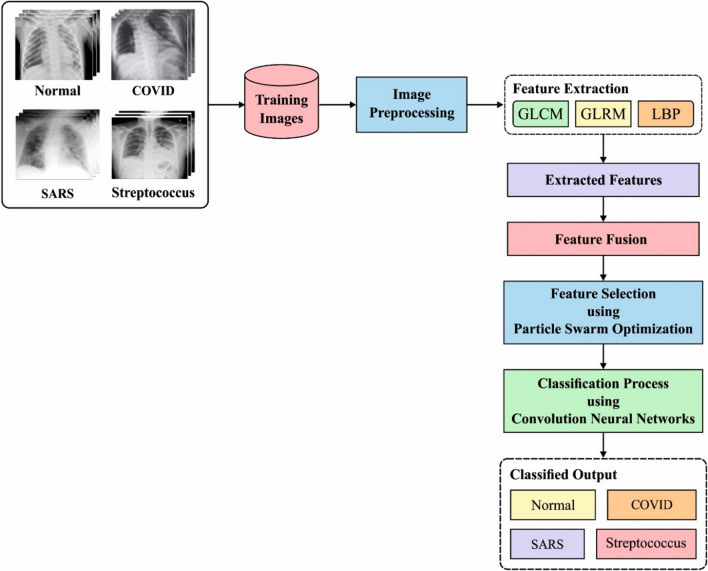
The working principle of the proposed FM-CNN model is shown in Fig. 1. The processes involved the method such as preprocessing, feature extraction, and classification processes are discussed in subsequent sections.
Fig. 1.
Block diagram of FM-CNN model
WF based preprocessing
Noise removal in the said image preprocessing operation improves the features of the image, interrupted by noise. Specifically, adaptive filtering is employed in which denoising is carried out on the basis of noise content that exists in the image. In Eq. 1, assume the image be while the noise variance of entire image is shown as Here, local mean is offered by in a pixel window and local variance from a window is denoted by . Next, a possible way of image denoising is defined as given herewith
| 1 |
Followed by, when noise variance over the image is 0 then it is changed as given herewith.
| 2 |
If global noise variance is low and local variance is high, then the global variance becomes 1; thus, If
| 3 |
The higher local variance showcases the occurrence of an edge from image window. For identical local as well as global variances, the notion is depicted herewith.
| 4 |
The predefined analogies illustrate a mean in which the output denotes the mean value of a window with no disorders. It is also an inherent functionality of WF. This filter uses window size as input and computes residual objectives (Vallabhaneni and Rajesh 2018). Hence, the achieved results infer that the noise is eliminated from CXR images with the help of WF. The main aim of this model is to know the result of WF noise removal on edges.
Fusion of feature extraction models
This section discusses the fusion of GLCM, GLRM, and LBP features to extract a group of feature vectors from the pre-processed CXR images. The optimal feature selection process is executed with the help of PSO algorithm among the features extracted from GLCM, GLRM, and LBP techniques.
GLCM features
GLCM is a general statistical method with spatial connection between the pixels (Raj et al. 2020). Being a histogram, it defines the importance of a pixel by particular distance in an image. Assume as the size of image, , with gray levels where and are two pixels with gray level intensities i.e., and , respectively. Followed by, in direction and in direction, the connecting line direction is similar to . The generalized ‐occurrence matrix is expressed as follows.
| 5 |
Here, is determined by . illustrates the value of modules in ‐occurrence matrix and denotes the number of pixels. Usually, and are implemented in estimations. These five different texture features are explained below in the function of ‐occurrence matrix.
| 6 |
| 7 |
| 8 |
| 9 |
| 10 |
where indicates the mean value of ‐occurrence matrix
GLRM features
In GLRLM, the homogeneous dimension runs to a gray level. It is defined with directions and texture indices attained from the matrix like short run, long run, gray level non‐uniformity, run-length non‐uniformity, run ratio, lower gray level run, higher gray level run, short run low gray level, short run high gray level, long run low gray level and long run high gray level. The module of GLRLM is equivalent to homogeneous runs of pixels with intensity from the image i.e., GLRLM . Considering the GLRM matrix with features as previously defined, the features and directions could be accomplished from all the images.
Where denotes a GLRM matrix, depicts a gray level, illustrates run length and indicates the sum of entire values in GLRM matrix.
| 11 |
| 12 |
| 13 |
| 14 |
| 15 |
| 16 |
| 17 |
| 18 |
| 19 |
| 20 |
LBP features
LBP is referred to as a statistical method used in image processing to examine the image features. It is executed mainly in computer vision applications. The operator develops a binary value for all pixels than center pixel and surrounding pixels over . LBP measures are carried out through binarization amongst the neighbours of pixels in all images by applying a function (Eq. (21)).
| 21 |
In equation, refers to radius and species of the distance from nearest pixels to intermediate pixels. However, implies the count of neighbor pixels. Uniform patterns are determined as binary LBP code i.e., 0–1 or 1–0 and the count of transition is 2. Uniform patterns determine the textures namely, spot, edge, and corner. It is also arranged as uniform patterns.
Optimal feature selection using PSO algorithm
Once the features are derived by three models, the optimum number of features is selected using PSO algorithm. It is based on bird flocking or fish shoaling nature. Every bird is signified as a point in Cartesian coordinate system which is allocated with primary velocity and position in a random fashion. Followed by, the system with adjacent proximity velocity maps the rule and is composed of similar speed as it is considered as the nearest neighbour. This method is elegant and is artificially configured with a random variable which is then included for increasing the efficiency. Besides, the closest proximity velocity match speed is enclosed with a random parameter that develops an overall simulation.
Heppner developed a cornfield method to simulate the foraging behaviour of a flock of birds. When a “cornfield model” is considered for a plane that includes food’s place, the birds are distributed randomly on the plane at initial stages. To identify the position of food, the birds are shifted according to the procedure.
Initially, the position coordinate of a cornfield is , while the position and velocity coordinates of a single bird are and , correspondingly. The distances among the recent positions and cornfield are employed to determine the function of recent position as well as speed. Moreover, the maximum distance of ‘cornfield’ shows enhanced performance or otherwise it becomes ineffective. Consider that every bird has a capability to remember and store its food at an optimal position once it reaches the destination which is named as pbest. denotes the velocity adjusting constant, rand implies an arbitrary value between [0,1], where a modified velocity item is fixed on the basis of given rules:
if pbestx, —rand , else,
if pbesty, —rand , else,
Then, the swarm communicates in any manner due to which an individual remembers the optimal position (gbest) among the overall swarm. Followed by, implies the velocity modifying constant; afterwards, the velocity item is tailored on the basis of provided rule which has to be maximized as given herewith.
if gbestx, —rand , else,
if gbesty, —rand , else,
The systematic outcomes imply that if is maximum, then every individual is gathered in ‘cornfield’ whereas, if is minimum, then the particles are clustered around the ‘cornfield’ gradually. Through better simulation, it is found that a swarm can identify the best point rapidly. As per the model developed by Kennedy and Eberhart, evolutionary optimization algorithm was applied in this study on a trial-and-error basis for which the equation is as follows.
| 22 |
Each individual is abstracted with no mass and volume along with velocity and position and is termed as PSO model.
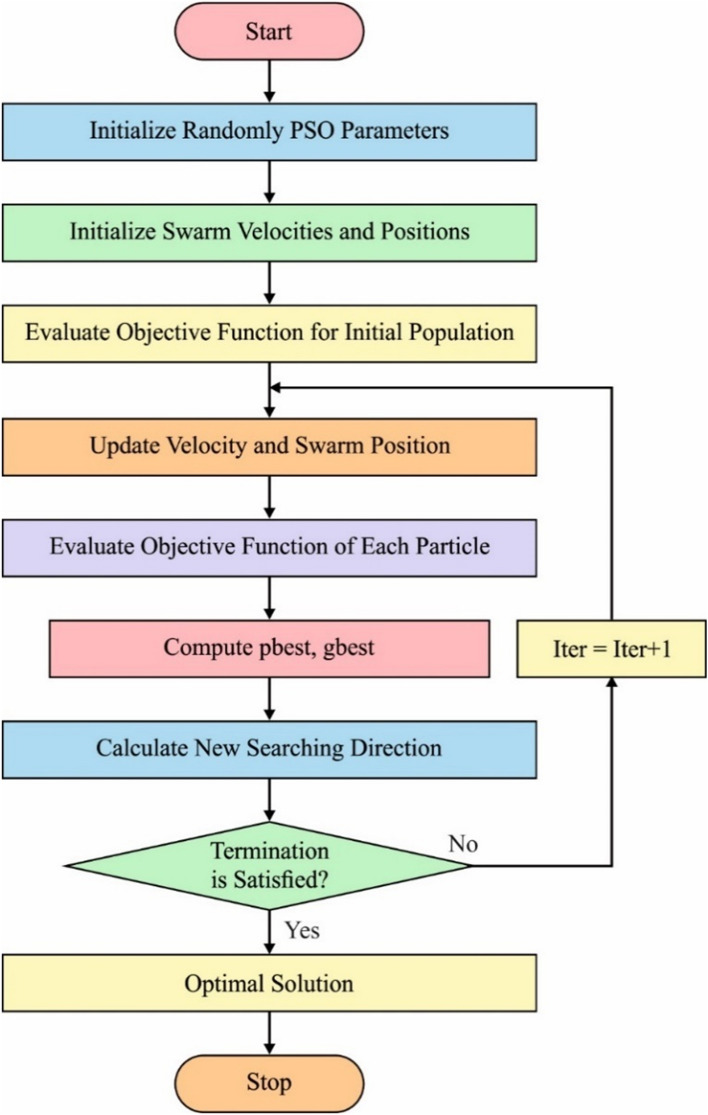
PSO approach is deemed to be an exploring task which depends upon the swarm, where every individual is named as a particle that provides a capable solution for optimized issues in ‐dimensional search space. It further remembers the best place in a swarm and its velocity. In every generation, the particle details are integrated to change the velocity of all dimensions applied so as to compute the position of a novel particle. The unique connection among different dimensions of the problem space is developed through objective functions. Various sorts of empirical evidence infer that this method is highly efficient in optimization. Figure 2 is the flowchart of PSO model.
Fig. 2.
Flowchart of PSO algorithm
The upcoming rules demonstrate the PSO method. In case of a continuous space coordinate system, PSO is defined as given herewith. Consider the swarm size as , every particle’s position vector in ‐dimensional space is , the velocity vector is , the individual’s best position is and swarm’s optimal position is . In the absence of generality, the initial version of the PSO approach upgrades the function of an individual’s best location by considering minimizing issues as the example.
| 23 |
The swarm’s best place is represented by the optimal location of the individual. Both notion of velocity and position are upgraded based on the equation given below.
| 24 |
| 25 |
As the initial method of PSO is not suitable for optimization issues, a modified PSO framework was developed by the researcher in this study. Inertia weight is also deployed to upgrade the velocity formula and is expressed as follows.
| 26 |
Though this modified technique is quite complicate alike the traditional model, there is an improvement observed in performance efficiency. Hence, it has gained some extended features. In general, the expanded version is named as canonical PSO method whereas PSO algorithm is the primary edition. The examination of convergence behavior of PSO method was established by Clerc and Kennedy (2002) with constriction factor that has assured convergence and enhanced the convergence rate. Next, the velocity update function is referred to as:
| 27 |
In fact, no significant variations were found between the iteration formulas, (26) and (27). At the time of selecting better variables, two functions are similar.
PSO approach is composed of two modules namely, global version and local version. In case of global version, two extremes are considered in which the particles track the best position pbest by its own and the optimal position gbest of a swarm. In case of local version, apart from tracking the optimal position pbest, the particle does not observe the swarm optimal position gbest. Instead, it monitors the particles’ optimal place nbest from topology neighbourhood. The velocity update is given in Eq. (26):
| 28 |
where denotes the maximum position. In all generations, the iteration of a particle is as depicted herewith.
Figure 2 examines the velocity update formula from sociological point of view. The formula impacts the former velocity of the particle. It refers that the particle is trusted on its confidence and performs inertial moving based on the velocity. So, the parameter is termed as inertia weight. Secondly, it relies on the distance between the particle’s recent position and best position, named as ‘cognitive’ item. Hence, parameter is named as cognitive learning factor. The third part depends on the distance between the particle’s recent position and global or local optimal position of a swarm referred to as ‘social’ factor. It is defined that the data is shared and cooperation exists between the particles alike how particle move from alternate particles’ experience in the swarm. It activates the movement of the best particle by cognition while the parameter is termed to be the social learning factor. Because of its intuitive background, it is simple to execute and it has extensive adaptability for diverse applications as the PSO model was developed with great response from many developers. In the last few decades, the theory and utilization of PSO model have accomplished optimal results.
The objective function of PSO algorithm is to minimize the objective function as defined below.
where ‘x’ denotes the vector of decision variables, is a function of is the number of objective functions to be minimized and and are the restraint functions of the problem.
COVID-19 disease classification
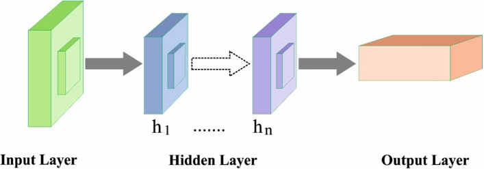
CNNs are defined as regular feedforward neural networks in which the neuron acquires inputs from the neurons present in traditional layer and enhances the input with network weights as well as performs nonlinear transformation. In contrast to NN, a neuron in CNN is linked with neurons in the former layer named as local receptive field. Furthermore, neurons are organized in 3D format in a layer with width, height and depth specifications. Initially, CNNs are developed for encoding spatial details accessible in images and making it as an effective network (Bejiga et al. 2017). The regular NN undergoes processing complexity and overfitting issues with enhanced input size. However, CNNs resolve these issues by weight distribution. Thus, weight distribution is a model where neurons in a ConvNet are limited with in-depth slice and applies weights and bias in spatial dimension. Therefore, the collection of learned weights is termed as filters or kernels. In general, CNN structure (Fig. 3) has a cascade of layers developed using Convolutional, Pooling, and FC layers.
Fig. 3.
Structure of CNN
Convolutional layer
This layer is the major building block of ConvNet and is composed of learnable filters. Such filters are minimum in number spatially and its dimension undergoes complete in-depth expansion. Through network training, filters activate neurons while at the same time, it detects special features spatially. Moreover, the convolution layer computes a convolution of input along with a filter and generates an outcome called activation map. Numerous filters are applied in single convolutional layer as well as activation maps of every stacked filter which induces the resultant layer to be an input for the upcoming layer. Furthermore, the size of the output is managed by three parameters namely, Depth, Stride, and Zero padding. Initially, the depth parameter is applied for managing the filters present in convolutional layer. Stride controls the expansion of overlap between adjacent receptive fields and impacts on the spatial dimension of resultant volume. Zero padding is employed to show the count of zeros which has to be padded on the edge of input that activates an input conservation. Though nonlinear activation functions are numerous in number, like sigmoid and tanh, the prominently applied ConvNets is Rectified Linear unit ReLu) which supports zero as input. ReLus is simple to execute whereas its non‐saturating format stimulates the convergence of SGD.
Pooling layer
CNNs apply pooling layers additionally to reduce overfitting problem. Here, the pooling layer computes spatial resizing. Alike convolutional layers, it is composed of a stride as well as filter size parameters to control the spatial size of final result. Every element in the activation map is equal to the aggregate statistics of an input spatially. The overfitting issues can be mitigated under the application of pooling layers after which it reaches a spatial invariance. Most of the frequently applied pooling tasks in CNNs are: (1) pooling, that proceeds with the highest response of provided patch; (2) average pooling, that determines the average response of the applied patch; and (3) sub-sampling, that estimates the average over a patch of size , enhances a tunable parameter , and a trainable bias , which employs a nonlinear function (Eq. (29)):
| 29 |
Fully connected layer
Fully connected layer is a regular Multi‐Layer Perceptron (MLP) which is employed for classification, where a neuron is linked to every neuron in the former layer. Afterward, the weights and biases are applied to know the variations of GD method. This model has to be processed with a loss function by means of network variables under backpropagation (BP) approach. In case of context classification, the cross‐entropy loss function has been employed in conjunction with softmax classifier.
When training deep CNN structures using large-scale training dataset, it demands high computing energy and time. Hence, an effective pre-trained scheme was employed in this study for certain operations by fine-tuning a feature extractor for prediction operation. Transfer learning is applied depending on the size of training dataset and the connection with actual dataset. Here, the commonly-accessible datasets are employed for training CNN i.e., so-called GoogLeNet. In this study, the GoogleNet model is chosen due to the following advantages. It significantly deepens and widens the network. It also minimizes the number of needed parameters and reduces the error rate. The training process of GoogleNet is faster than the VGG and it is also smaller Ilar n size.
It can be trained in image classification operations with ImageNet ILSVRC2014 challenge and can be graded initially. Some of the challenging issues are classification of images in massive numbers lead to node classes in ImageNet hierarchy. ILSVRC dataset is comprised of numerous images which are used for training, validation, and testing. Every convolutional layer has filters of high size from to and applies a ReLu activation function. The max pooling kernels, in the range of with average pooling kernel size , were employed in the current study as a diverse system. Hence, the input layer is consuming a color image sized . On the other hand, a better classification function is accomplished by the system. A deep architecture model assumes that the energy and storage of movable and incorporated platforms are used in real-world applications in a cost-effective manner.
Performance validation
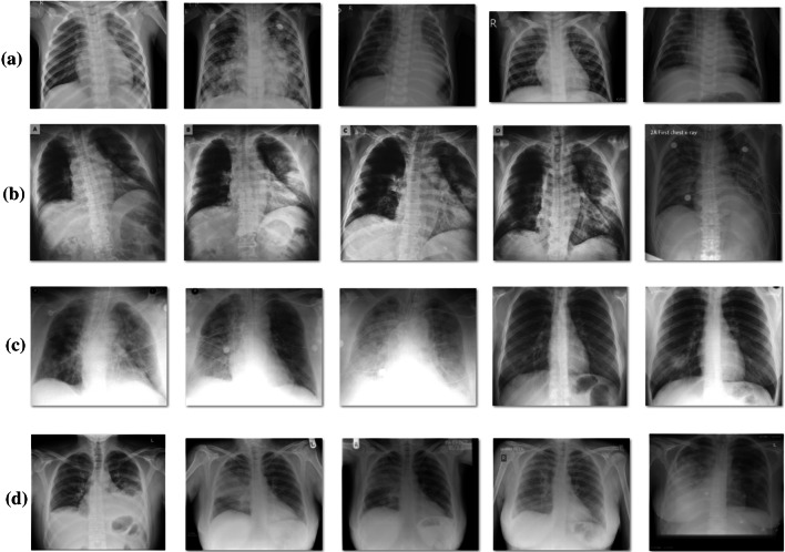
This section discusses the performance of FM-CNN model on the diagnosis of COVID-19 using CXR dataset (Cohen et al. 2020; https://github.com/ieee8023/covid-chestxray-dataset). The CXR dataset includes a total of 27 images under normal, 220 images under SARS, and 17 images under Streptococcus. Figure 4 illustrates a few sample CXR images grouped under multiple classes.
Fig. 4.
Multi-Class a Normal b COVID-19 c SARS d Streptococcus
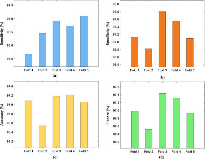
Table 1 and Fig. 5 illustrate the binary classification performance of FM-CNN method on the applied CXR images under varying number of folds. In applied fold 1, the FM-CNN model obtained a high sensitivity of 95.67%, specificity of 97.13%, accuracy of 97.08%, and F-score of 96.98%. In applied fold 2, the FM-CNN method accomplished the maximum sensitivity of 96.45%, specificity of 96.82%, accuracy of 96.54%, and F-score of 96.52%. In terms of applied fold 3, the FM-CNN approach attained a high sensitivity of 96.91%, specificity of 97.80%, accuracy of 97.18%, and F-score of 97.43%. Further, the FM-CNN framework achieved better sensitivity of 96.72%, specificity of 97.54%, accuracy of 97.21%, and F-score of 97.31% in applied fold 4. Finally, in applied fold 5, the FM-CNN scheme obtained an optimal sensitivity of 97.10%, specificity of 97.09%, accuracy of 97.05%, and F-score of 96.92%.
Table 1.
Results of FM-CNN model for binary class in terms of different measures
| No. of folds | Sensitivity | Specificity | Accuracy | F-score |
|---|---|---|---|---|
| Fold 1 | 95.67 | 97.13 | 97.08 | 96.98 |
| Fold 2 | 96.45 | 96.82 | 96.54 | 96.52 |
| Fold 3 | 96.91 | 97.80 | 97.18 | 97.43 |
| Fold 4 | 96.72 | 97.54 | 97.21 | 97.31 |
| Fold 5 | 97.10 | 97.09 | 97.05 | 96.92 |
| Average | 96.57 | 97.28 | 97.01 | 97.03 |
Fig. 5.
Binary class analysis of FM-CNN model
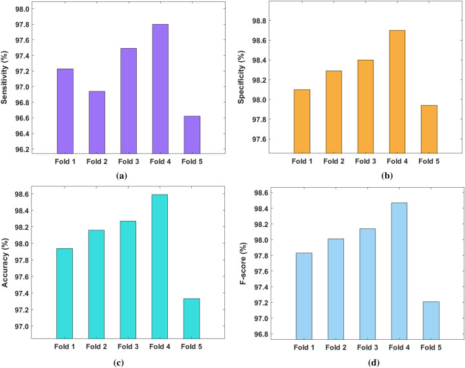
Table 2 and Fig. 6 demonstrate the multi-class classification function of FM-CNN method on the applied CXR images under diverse number of folds. In applied fold 1, the FM-CNN method achieved the maximum sensitivity of 97.23%, specificity of 98.10%, accuracy of 97.94%, and F-score of 97.83%. Furthermore, in applied fold 2, the FM-CNN framework accomplished a better sensitivity of 96.94%, specificity of 98.29%, accuracy of 98.16% and F-score of 98.01%.
Table 2.
Results of FM-CNN model for multi class in terms of different measures
| No. of folds | Sensitivity | Specificity | Accuracy | F-score |
|---|---|---|---|---|
| Fold 1 | 97.23 | 98.10 | 97.94 | 97.83 |
| Fold 2 | 96.94 | 98.29 | 98.16 | 98.01 |
| Fold 3 | 97.49 | 98.40 | 98.27 | 98.14 |
| Fold 4 | 97.80 | 98.70 | 98.59 | 98.47 |
| Fold 5 | 96.62 | 97.94 | 97.33 | 97.21 |
| Average | 97.22 | 98.29 | 98.06 | 97.93 |
Fig. 6.
Multi class analysis of FM-CNN model
In addition, from applied fold 3, the FM-CNN approach gained good sensitivity of 97.49%, specificity of 98.40%, accuracy of 98.27%, and F-score of 98.14%. Moreover, in applied fold 4, the FM-CNN method achieved the maximum sensitivity of 97.80%, specificity of 98.70%, accuracy of 98.59%, and F-score of 98.47%. Finally, the FM-CNN model attained an optimal sensitivity of 96.62%, specificity of 97.94%, accuracy of 97.33%, and F-score of 97.21% in applied fold 5.
Figure 7 portrays the results of average analysis of FM-CNN model in terms of CXR image classification. In binary classification of CXR images, the proposed FM-CNN model demonstrated superior performance with average sensitivity of 96.57%, specificity of 97.28%, accuracy of 97.01%, and F-score of 97.03%. Besides, the presented FM-CNN model resulted in high average sensitivity of 97.22%, specificity of 98.29%, accuracy of 98.06%, and F-score of 97.93% in multi-classification of CXR images.
Fig. 7.
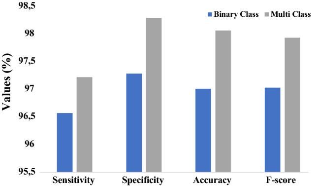
Average analysis of FM-CNN model
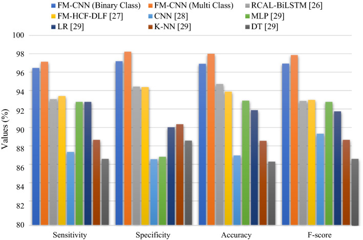
Table 3 and Fig. 8 provides a detailed results of the comparison made between FM-CNN model and the existing methods (Pustokhin et al. 2020; Shankar and Perumal 2020; Pathak et al. 2020; Mondal et al. 2020) in terms of distinct measures. When comparing the results achieved by FM-CNN against existing models, CNN, KNN, and DT models accomplished a minimum classification performance. However, MLP and LR models exhibited slightly higher and closer classification performance. Furthermore, the Resnet-50, VGG-19, VGG-16, AlexNet, RCAL-BiLSTM and FM-HCF-DLF models demonstrated somewhat acceptable results. However, the FM-CNN model outperformed all the methods compared by achieving the maximum accuracy of 97.01% and 98.06% on the classification of binary and multiple classes respectively.
Table 3.
Comparative analysis of existing methods against the proposed FM-CNN method
| Methods | Sensitivity | Specificity | Accuracy | F-score |
|---|---|---|---|---|
| FM-CNN (Binary Class) | 96.57 | 97.28 | 97.01 | 97.03 |
| FM-CNN (Multi Class) | 97.22 | 98.29 | 98.06 | 97.93 |
| Resnet-50 Model | 96.54 | 96.72 | 96.21 | 96.56 |
| VGG-19 Model | 96.10 | 96.24 | 96.18 | 96.15 |
| VGG-16 Model | 95.98 | 95.87 | 95.92 | 95.85 |
| AlexNet Model | 94.76 | 95.18 | 95.64 | 95.09 |
| RCAL-BiLSTM (Pustokhin et al. 2020) | 93.28 | 94.61 | 94.88 | 93.10 |
| FM-HCF-DLF (Shankar and Perumal 2020) | 93.61 | 94.56 | 94.08 | 93.20 |
| CNN (Pathak et al. 2020) | 87.73 | 86.97 | 87.36 | 89.65 |
| MLP (Mondal et al. 2020) | 93.00 | 87.23 | 93.13 | 93.00 |
| LR (Mondal et al. 2020) | 93.00 | 90.34 | 92.12 | 92.00 |
| K-NN (Mondal et al. 2020) | 89.00 | 90.65 | 88.91 | 89.00 |
| DT (Mondal et al. 2020) | 87.00 | 88.93 | 86.71 | 87.00 |
Fig. 8.
Comparative results analysis of the FM-CNN with existing methods
Conclusion
The current research article introduced an automated COVID-19 diagnosis process using FM-CNN model. The proposed FM-CNN model had three stages namely, preprocessing, feature extraction, and classification. Primarily, the input CXR images were pre-processed using WF technique, and the features were extracted using FM technique. Then, the optimal features were selected using PSO algorithm. At last, the CNN model was applied as a classifier to identify the existence of binary and multiple classes present in CXR images. The performance of FM-CNN model was validated using benchmark CXR images and the results were investigated in terms of several aspects. In the experimentation procedure, the FM-CNN model classified multiple classes with maximum sensitivity of 97.22%, specificity of 98.29%, accuracy of 98.06%, and F-measure of 97.93%. Therefore, the current study established the superiority of FM-CNN model as an appropriate tool for COVID-19 diagnosis and classification. In future, the performance of FM-CNN model can be improved by using hyperparameter tuning models for CNN.
Declarations
Conflict of interest
The authors declare that they have no conflict of interest. The manuscript was written through contributions of all authors. All authors have given approval to the final version of the manuscript.
Footnotes
Publisher's Note
Springer Nature remains neutral with regard to jurisdictional claims in published maps and institutional affiliations.
Contributor Information
K. Shankar, Email: drkshankar@ieee.org
Sachi Nandan Mohanty, Email: Sachinandan09@gmail.com.
Kusum Yadav, Email: Y.kusum@uoh.edu.sa.
T. Gopalakrishnan, Email: gopalakrishnan.t@vit.ac.in
Ahmed M. Elmisery, Email: amelmesiry@gmail.com
References
- Abbas A, Abdelsamea MM, Gaber MM. Classification of COVID-19 in chest x-ray images using DeTraC deep convolutional neural network. Appl Intell. 2020;51:854–864. doi: 10.1007/s10489-020-01829-7. [DOI] [PMC free article] [PubMed] [Google Scholar]
- Apostolopoulos ID, Mpesiana TA. Covid-19: automatic detection from X-ray images utilizing transfer learning with convolutional neural networks. Phys Eng Sci Med. 2020;43(2):635–640. doi: 10.1007/s13246-020-00865-4. [DOI] [PMC free article] [PubMed] [Google Scholar]
- Barstugan M, Ozkaya U, Ozturk S (2020) Coronavirus (COVID-19) classification using CT images by machine learning methods
- Bejiga MB, Zeggada A, Nouffidj A, Melgani F. A convolutional neural network approach for assisting avalanche search and rescue operations with UAV imagery. Remote Sens. 2017;9(2):100. doi: 10.3390/rs9020100. [DOI] [Google Scholar]
- Butt C, Gill J, Chun D, Babu BA. Deep learning system to screen coronavirus disease 2019 pneumonia. Appl Intell. 2020;6:1–7. doi: 10.1007/s10489-020-01714-3. [DOI] [PMC free article] [PubMed] [Google Scholar]
- Clerc M, Kennedy J. The particle swarm: explosion, stability, and convergence in a multi- dimensional complex space. IEEE Trans Evol Comput. 2002;6:58–73. doi: 10.1109/4235.985692. [DOI] [Google Scholar]
- Cohen JP, Morrison P, Dao L, Roth K, Duong TQ, Ghassemi M (2020) Covid-19 image data collection: prospective predictions are the future. arXiv preprint arXiv:2006.11988
- Elmisery AM, Sertovic M. Privacy enhanced cloud-based recommendation service for implicit discovery of relevant support groups in healthcare social networks. Int J Grid High Perform Comput IJGHPC. 2017;9(1):75–91. doi: 10.4018/IJGHPC.2017010107. [DOI] [Google Scholar]
- Elmisery AM, Rho S, Botvich D. A distributed collaborative platform for personal health profiles in patient-driven health social network. Int J Distrib Sens Netw. 2015 doi: 10.1155/2015/406940. [DOI] [Google Scholar]
- Gaber MM, Aneiba A, Basurra S, et al. Internet of things and data mining: from applications to techniques and systems. Wires Data Min Knowl Discov. 2019;9:e1292. doi: 10.1002/widm.1292. [DOI] [Google Scholar]
- Ghoshal B, Tucker A, Sanghera B, Wong WL (2019) Estimating uncertainty in deep learning for reporting confidence to clinicians when segmenting nuclei image data. In: Proceedings—IEEE symposium on computer-based medical systems, pp 318–24
- Gozes O et al (2020) Rapid AI development cycle for the coronavirus (COVID-19) pandemic: initial results for automated detection and patient monitoring using deep learning CT image analysis
- Hall LO, Paul R, Goldgof DB, Goldgof GM (2020) Finding Covid-19 from chest x-rays using deep learning on a small dataset
- Hemdan EE-D, Shouman MA, Karar ME (2020) COVIDX-Net: a framework of deep learning classifiers to diagnose COVID-19 in x-ray images
- Imran A, et al. AI4COVID-19: AI enabled preliminary diagnosis for COVID-19 from cough samples via an app. Inf Med Unlocked. 2020;20:100378. doi: 10.1016/j.imu.2020.100378. [DOI] [PMC free article] [PubMed] [Google Scholar]
- Le DN, Parvathy VS, Gupta D, Khanna A, Rodrigues JJ, Shankar K. IoT enabled depthwise separable convolution neural network with deep support vector machine for COVID-19 diagnosis and classification. Int J Mach Learn Cybern. 2021;2:1–14. doi: 10.1007/s13042-020-01248-7. [DOI] [PMC free article] [PubMed] [Google Scholar]
- Lecun Y, Bengio Y, Hinton G. Deep learning. Nature. 2015;521(7553):436–444. doi: 10.1038/nature14539. [DOI] [PubMed] [Google Scholar]
- Li L, et al. Artificial intelligence distinguishes COVID-19 from community acquired pneumonia on chest CT. Radiology. 2020;296:200905. doi: 10.1148/radiol.2020200905. [DOI] [PMC free article] [PubMed] [Google Scholar]
- Mahase E. Coronavirus COVID-19 has killed more people than SARS and MERS combined, despite lower case fatality rate. BMJ. 2020;368:m641. doi: 10.1136/bmj.m641. [DOI] [PubMed] [Google Scholar]
- Mondal MRH, Bharati S, Podder P, Podder P. Data analytics for novel coronavirus disease. Inf Med Unlocked. 2020;20:100374. doi: 10.1016/j.imu.2020.100374. [DOI] [PMC free article] [PubMed] [Google Scholar]
- Narin A, Kaya C, Pamuk Z. Automatic detection of coronavirus disease (COVID-19) using x-ray images and deep convolutional neural networks. Pattern Anal Appl. 2020;24:1207–1220. doi: 10.1007/s10044-021-00984-y. [DOI] [PMC free article] [PubMed] [Google Scholar]
- Pathak Y, Shukla PK, Tiwari A, Stalin S, Singh S. Deep transfer learning based classification model for COVID-19 disease. Irbm. 2020;1:1–6. doi: 10.1016/j.irbm.2020.05.003. [DOI] [PMC free article] [PubMed] [Google Scholar]
- Pustokhin DA, Pustokhina IV, Dinh PN, Phan SV, Nguyen GN, Joshi GP. An effective deep residual network based class attention layer with bidirectional LSTM for diagnosis and classification of COVID-19. J Appl Stat. 2020;8:1–18. doi: 10.1080/02664763.2020.1849057. [DOI] [PMC free article] [PubMed] [Google Scholar]
- Raj RJS, Shobana SJ, Pustokhina IV, Pustokhin DA, Gupta D, Shankar K. Optimal feature selection-based medical image classification using deep learning model in internet of medical things. IEEE Access. 2020;8:58006–58017. doi: 10.1109/ACCESS.2020.2981337. [DOI] [Google Scholar]
- Sabour S, Frosst N, Hinton GE (2017) Dynamic routing between capsules
- Salman FM, Abu-Naser SS, Alajrami E, Abu-Nasser BS, Ashqar BAM. COVID-19 detection using artificial intelligence. Int J Acad Eng Res. 2020;4(3):18–25. [Google Scholar]
- Sethy PK, Behera SK, Ratha PK, Biswas P. Detection of coronavirus disease (COVID-19) based on deep features. Int J Math Eng Manag Sci. 2020;5(4):643–651. [Google Scholar]
- Shankar K, Perumal E. A novel hand-crafted with deep learning features based fusion model for COVID-19 diagnosis and classification using chest X-ray images. Complex Intell Syst. 2020;7:1–17. doi: 10.1007/s40747-020-00216-6. [DOI] [PMC free article] [PubMed] [Google Scholar]
- Vallabhaneni RB, Rajesh V. Brain tumour detection using mean shift clustering and GLCM features with edge adaptive total variation denoising technique. Alex Eng J. 2018;57(4):2387–2392. doi: 10.1016/j.aej.2017.09.011. [DOI] [Google Scholar]
- Wang L, Wong A. COVID-Net: a tailored deep convolutional neural network design for detection of COVID-19 cases from chest X-Ray images. Sci Rep. 2020;10:1–12. doi: 10.1038/s41598-020-76550-z. [DOI] [PMC free article] [PubMed] [Google Scholar]
- Zhang J, Xie Y, Li Y, Shen C, Xia Y (2020) COVID-19 screening on chest x-ray images using deep learning based anomaly detection
- Zheng C et al (2020) Deep learning-based detection for COVID-19 from chest CT using weak label. medRxiv 03.12.20027185


