Abstract
Artificial intelligence and machine learning are employed in creating functions for the prediction of self-compacting concrete (SCC) strength based on input variables proportion as cement replacement. SCC incorporating waste material has been used in learning approaches. Artificial neural network (ANN) support vector machine (SVM) and gene expression programming (GEP) consisting of 300 datasets have been utilized in the model to foresee the mechanical property of SCC. Data used in modeling consist of several input parameters such as cement, water–binder ratio, coarse aggregate, fine aggregate, and fly ash (FA) in combination with the superplasticizer. The best predictive models were selected based on the coefficient of determination (R2) results and model validation. Empirical relation with mathematical expression has been proposed using ANN, SVM, and GEP. The efficiency of the models is assessed by permutation features importance, statistical analysis, and comparison between regression models. The results reveal that the proposed machine learning models achieved adamant accuracy and has elucidated performance in the prediction aspect.
Keywords: self-compacting concrete, fly ash, machine learning, artificial neural network, gene engineering programming
1. Introduction
In recent years, concrete technology has been improving due to the fact that it is the most commonly used building material in the world. The knowledge of advance techniques of designing concrete has also improved recently due to different type of concrete being designed containing different admixtures [1]. One of the results of developing concrete designing technology is self-compacting concrete (SCC) [2]. Self-compacting concrete is defined as a cementitious material that can flow under its own weight and was first developed in the late 1990s in Japan. SCC deforms efficiently and shows maximum resistance to segregation and bleeding as per American Concrete Institute committee 237 R-07 [3]. Moreover, due to its workability, SCC is more often used where there is a need of creating different shapes of the elements or there are some parts of elements hardly reachable [4].
SCC is an advanced material with similar strength and durability as compared with traditional vibrated concrete; however, very often, due to self-venting, it is characterized by better performance; thus, it is sometimes used in strengthening of reinforced concrete (RC) beams [5,6]. Even though the SCC is commonly used in construction practice, designing proper mixture of SCC is still a difficult task to solve. The main reason of this is the fact that concrete itself is a quasi-brittle material [7]; the SCC requires relevant flow, and more often, industrial wastes are added as by-products: fly ash (FA), silica fume (SF), and ground granulated blast furnace slag (GGBFS) [8]. There are certain waste byproducts that, when included in the cementitious system as a partial replacement of cement, substantially reduce the desired energy and CO2 emission [9].
In light of sustainable development and waste management, investigating the influence of the addition of the aforementioned by-products on cementitious composites properties should not be neglected. Fly ash is a fine-grained dust, consisting mainly of spherical, vitrified grains obtained by burning pulverized coal with or without co-incineration, showing pozzolanic properties and mainly containing Al2O3 and SiO2. Fly ash may be used in the production of concrete if it meets the requirements included in the standards [10]. The use of fly ash in concrete brings many benefits, such as: completing the particle size distribution curve, increasing the final strength of concrete as a result of the pozzolanic activity of fly ash, compacting the microstructure, and easier displacement of aggregate grains in relation to each other, which is the essence of a fresh self-compacting concrete mixture [11].
The SCC’s complex structure requires a rigorous mixed design process for achieving its required properties. The SCC mixture can differ, when analyzing the literature, due to variations in the quantity and quality of mineral admixtures, as well as design standards. What is more, the general relationship between the binder ratio to mineral admixtures, chemical admixtures, w/b ratio, and aggregate particle size seems to be ambiguous. Meanwhile, traditional methods were used by many researchers in achieving SCC properties, but the modeling aspect and optimization of mineral admixture are still missing in most aspects [12].
Computation methods as well as machine learning techniques have recently become a powerful way of modeling and estimating an extensive series of problems, particularly in modeling concrete properties [13,14,15]. Numerous studies have been conducted in the prediction of mechanical properties of self-compacting concrete and some selected of the latest, together with the name of the applied machine learning algorithm and used waste material, are listed in Table 1.
Table 1.
The latest works in the subject of concrete compressive strength prediction.
| S. No | Algorithm Name | Notation | Dataset | Prediction Properties | Year | Waste Material Used | References |
|---|---|---|---|---|---|---|---|
| 1 | Artificial neural network | ANN | 169 | Compressive strength | 2016 | FA GGBFS SF RHA |
[16] |
| 2 | Artificial neural network | ANN | 205 | Compressive strength | 2019 | FA GGBFS SF RHA |
[17] |
| 3 | Artificial neural network | ANN | 114 | Compressive strength | 2017 | FA | [18] |
| 4 | Artificial neural network | ANN | 80 | Compressive strength | 2011 | FA | [19] |
| 5 | Artificial neural network | ANN | 300 | Compressive strength | 2009 | FA | [20] |
| 6 | Support vector machine | SVM | - | Compressive strength | 2020 | FA | [21] |
| 7 | Random forest | RF | 131 | Compressive strength | 2019 | FA GGBFS SF |
[22] |
| 8 | Biogeographical-based programming | BBP | 413 | Elastic modulus | 2016 | SF FA SLAG |
[23] |
| 9 | Intelligent rule-based enhanced multiclass support vector machine and fuzzy rules | IREMSVM-FR with RSM |
114 | Compressive strength | 2019 | FA | [24] |
| 10 | Support vector machine | SVM | 115 | Slump test L-box test V-funnel test Compressive strength |
2020 | FA | [25] |
| 11 | Multivariate adaptive regression spline | M5 MARS |
114 | Compressive strength Slump test L-box test V-funnel test |
2018 | FA | [26] |
Despite the fact that researchers are implementing machine learning algorithms in concrete investigations, there is a lack of works focusing on models predicting the compressive strength of SCC modified with FA using comparative analyses containing artificial neural networks (ANN), support vector machine (SVM) and gene expression programming (GEP) combined. Taking into account the information presented in the Table 1, there is lack of comparative analysis of different machine learning algorithms used for self-compacting concrete compressive strength prediction. Thus, the aim of this study is to perform such analysis using ANN, SVM, and GEP and also to compare the obtained results with similar scientific works presented in the literature.
2. Research Significance
The novelty of this research is the usage of the newest machine learning algorithms in the comparative manner in order to evaluate the compressive strength of fly ash-based self-compacting concrete. For this purpose, the artificial neural network, support vector machine, and genetic expression programming were used. In particular, the novelty of this research is the usage of the genetic expression programming for this purpose. The best model among those investigated was selected after optimization. Permutation features and statistical analysis with in-depth error measures are conducted to compare the accuracy of aforementioned models and comparing them with others in the scientific field.
3. Prediction Methods
3.1. Artificial Neural Network (ANNs)
Artificial neural networks are algorithms simulating the microstructure (neurons) of a biological nervous system [27,28,29]. Their structure is similar to the biological connection between neurons in the human brain. The ANNs consist of layers: input (consist of variables used in order to forecast the investigated property), hidden (consist of nodes connected with other layers using functions and weights) and output (which is consist of predicted variables). It is possible to analyze data using ANN thanks to learning algorithms such as: quasi-Newtons, Levenberg–Marquardt’s and conjugate gradients [8]. ANNs are widely used in many applications and can therefore be a useful tool in engineering applications [30].
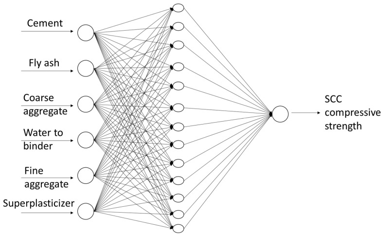
In this study, a multi-layer perceptron (MLP) feed-forward with backpropagation algorithm ANNs have been selected. One hidden layer and varying neuron numbers are selected to find the optimum performance of the multilayer perceptron neuron network (MLPNN) [31]. The learning algorithms used in ANNs modeling of SCC compressive strength were the Broyden–Fletcher–Goldfarb–Shano algorithm and the Levenberg–Marquardt algorithm. The data set division was fixed as: 70% of data was used in training process and 30% of data was used in processes of testing and validation [32]. Moreover, optimization of the training, validation set, and training set was obtained by changing the number of neuron layers with iteration, and vice versa. The most accurate results were obtained for the topology of six inputs, 13 hidden neurons, and one output. The topology of this network is presented in Figure 1 and described in Table 2.
Figure 1.
The topology of the neural network used in the study.
Table 2.
Neural network properties.
| Parameter | Neural Network Properties |
|---|---|
| Input parameters | Six (6) |
| Output parameters | One (1) |
| Percentage of training set/testing and validation set | 70/30 |
| Number of epochs | Hundred (100) |
| Performance limit | 10−6 |
| Training model | Supervised |
| Training process | Quasi-Newton |
| Activation function (HL) | Logistic (sigmoid) |
| Activation function (OL) | Logistic (linear) |
3.2. Support Vector Machine (SVM)
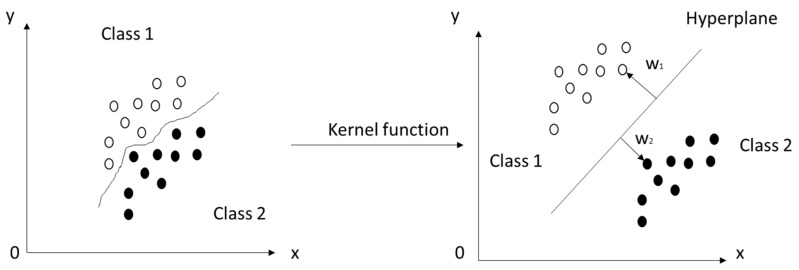
The support vector machine is a supervised learning model used for analyzing classification and regression data, invented by Vapnik [33]. The data are represented as a map of points in space and the solution is the hyperplane (lane in 2D, plane in 3D, etc.) with the widest possible gap between two classes. Each point in this space is described with support vectors; however, there are some situations wherein the division of the data set is possible only after using kernel functions, presented in Figure 2.
Figure 2.
Graphical interpretation of support vector machine method.
The support vector machine has been successfully used in solving some engineering problems, e.g., analyzing the durability of lightweight cement composites with hydrophobic coatings modified by nanocellulose [33]. In this work, the v-SVM was used, with linear kernel function as the most accurate. The other kernel function tested: polynomial, RBF, or sigmoid were not that significantly accurate.
3.3. Genetic Engineering Programming (GEP)
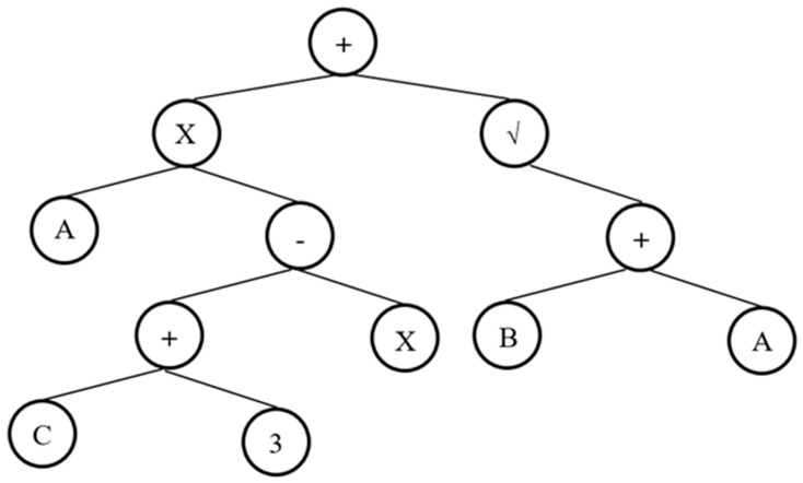
Genetic engineering programming is a versatile approach as it incorporates both gene algorithms (GAs) and genetic programming (GP) [34]. This algorithm consisting of trees, that are called expression trees (ETs), and the benefit of this solution is the fact of adamantly simplified at the chromosome level operation of genetic work [35]. Another modification in GEP, in comparison to GAs, is that the individual chromosomes that contain numerous genes and are additionally classified into the model head and tail [36]. Each individual gene of GEP, presented as a node of the ET, stores a number of variables with constant length, function set, and terminal sets. Function set, terminal set, and variables are connected with each other via a linear genetic code. It is worth mentioning here that these sets must have closure property. A sample of the GEP gene can also be represented by an expression tree (ETs) diagram. An example of ET diagram is shown in Figure 3.
Figure 3.
An example of tree expression (ETs).
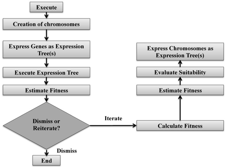
It is expected that every gene (chromosome) contains the head, which executes the algorithm by creating chromosomes. The individuals (gene) in GEP are selected and represented as expression tree(s) with the execution of the analysis. After performing the analysis, the fitness is estimated; based on this, the decision of dismissing or reiterating is made. Dismissing the fitness finishes the algorithm, while, during reiteration, the fitness is calculated and estimated once again in order to evaluate the suitability for another expression of chromosomes as expression trees. The schematic diagram of the GEP algorithm is shown in Figure 4.
Figure 4.
Schematic diagram of GEP algorithm.
4. Data Presentation
4.1. Correlation Graph Python Programming Based
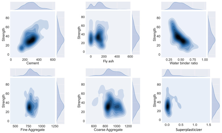
The collected SCC database taken from published literature [17,37,38,39,40,41,42,43,44,45,46,47,48,49,50,51,52,53,54,55,56,57,58,59,60] includes information on the water–binder ratio, fly ash, fine and coarse aggregate, superplasticizer, and cement content (see Appendix A). Each model performance is governed by the distribution of its parameters [61]. It can be seen that machine learning and artificial intelligence are hand full tools in the prediction of mechanical properties of SCCs. The distribution and relationship (optimal quantities) of input parameters to its output can be seen in contour form in Figure 5. It can be seen that with the increasing value of cement content, the compressive strength value has also increased; however, it is the opposite in the case the of water–binder ratio, wherein the increase of this ratio results in a decrease in compressive strength. Moreover, using these variable concentrations in SCCs yield maximum compressive strength output, thus eliminating its need for going in hit and trial methods to obtain the target strength. Furthermore, the range and description of data is shown in Table 3 and Table 4. It may be concluded that machine learning and deep learning approaches adamantly benefit in the prediction of the mechanical aspect of SCCs.
Figure 5.
Concentration of input variables in achieving maximum compressive strength of SCC.
Table 3.
Range of input and output variables.
| Parameters | Minimum | Maximum |
| Input Variables | ||
| Cement (kg/m3) | 83 | 540 |
| Fly ash (kg/m3) | 0 | 525 |
| Coarse aggregate (kg/m3) | 578 | 1125 |
| Fine aggregate (kg/m3) | 478 | 1180 |
| Superplasticizer (%) | 0 | 1.36 |
| Water–binder ratio | 0.22 | 0.9 |
| Output Variable | Minimum | Maximum |
| Compressive strength (MPa) | 8.54 | 78.4 |
Table 4.
The dataset from the latest works in the subject of concrete compressive strength prediction.
| Statistical Measures of Input Parameters and Output Strength in Modeling Prediction | ||||||
|---|---|---|---|---|---|---|
| Dataset | Parameters | |||||
| Training Set | Cement | Fly Ash | Water–Binder | Fine Aggregate | Coarse Aggregate | Superplasticizer |
| Mean | 292.48 | 118.08 | 0.48 | 802.90 | 912.45 | 0.18 |
| Standard Error | 6.69 | 6.13 | 0.01 | 6.76 | 7.82 | 0.02 |
| Median | 290.00 | 120.68 | 0.46 | 793.46 | 900.00 | 0.05 |
| Mode | 250.00 | 0.00 | 0.55 | 742.00 | 837.00 | 0.00 |
| Standard Deviation | 96.95 | 88.88 | 0.13 | 97.97 | 113.39 | 0.26 |
| Sample Variance | 9399.46 | 7899.70 | 0.02 | 9598.18 | 12,857.39 | 0.07 |
| Kurtosis | −0.11 | 2.55 | 0.26 | 2.30 | 0.27 | 3.89 |
| Skewness | 0.51 | 0.87 | 0.76 | 0.57 | −0.35 | 2.00 |
| Range | 457.00 | 525.00 | 0.67 | 693.00 | 547.00 | 1.36 |
| Minimum | 83.00 | 0.00 | 0.23 | 487.00 | 578.00 | 0.00 |
| Maximum | 540.00 | 525.00 | 0.90 | 1180.00 | 1125.00 | 1.36 |
| Sum | 61,421.24 | 24,796.10 | 100.81 | 168,608.70 | 191,614.79 | 37.16 |
| Count | 210.00 | 210.00 | 210.00 | 210.00 | 210.00 | 210.00 |
| Validation Set | Cement | Fly Ash | Water–Binder | Fine Aggregate | Coarse Aggregate | Superplasticizer |
| Mean | 292.65 | 117.73 | 0.49 | 789.71 | 912.83 | 0.18 |
| Standard Error | 13.13 | 13.29 | 0.02 | 15.47 | 18.82 | 0.04 |
| Median | 295.90 | 107.25 | 0.50 | 784.50 | 879.00 | 0.04 |
| Mode | 250.00 | 0.00 | 0.55 | 774.00 | 837.00 | 0.00 |
| Standard Deviation | 89.07 | 90.14 | 0.13 | 104.91 | 127.67 | 0.27 |
| Sample Variance | 7933.73 | 8125.93 | 0.02 | 11,005.42 | 16,300.13 | 0.07 |
| Kurtosis | 1.04 | −1.12 | −0.41 | 3.03 | −0.04 | 4.61 |
| Skewness | 0.65 | 0.09 | 0.03 | −0.08 | −0.22 | 2.07 |
| Range | 396.40 | 275.00 | 0.58 | 657.00 | 535.00 | 1.25 |
| Minimum | 143.60 | 0.00 | 0.22 | 478.00 | 590.00 | 0.00 |
| Maximum | 540.00 | 275.00 | 0.80 | 1135.00 | 1125.00 | 1.25 |
| Sum | 13,461.90 | 5415.63 | 22.52 | 36,326.78 | 41,989.96 | 8.22 |
| Count | 46.00 | 46.00 | 46.00 | 46.00 | 46.00 | 46.00 |
| Test Set | Cement | Fly Ash | Water–Binder | Fine Aggregate | Coarse Aggregate | Superplasticizer |
| Mean | 292.76 | 101.57 | 0.49 | 837.83 | 912.01 | 0.15 |
| Standard Error | 12.53 | 11.32 | 0.02 | 13.30 | 20.65 | 0.03 |
| Median | 290.00 | 100.37 | 0.51 | 808.00 | 940.60 | 0.03 |
| Mode | 250.00 | 0.00 | 0.33 | 899.00 | 837.00 | 0.00 |
| Standard Deviation | 84.02 | 75.94 | 0.13 | 89.20 | 138.54 | 0.22 |
| Sample Variance | 7059.62 | 5767.29 | 0.02 | 7956.13 | 19,193.24 | 0.05 |
| Kurtosis | −0.76 | −0.93 | −1.03 | 2.35 | −0.75 | 1.99 |
| Skewness | 0.09 | 0.03 | 0.02 | 1.21 | −0.45 | 1.66 |
| Range | 340.30 | 263.00 | 0.46 | 473.00 | 490.00 | 0.80 |
| Minimum | 134.70 | 0.00 | 0.27 | 662.00 | 621.00 | 0.00 |
| Maximum | 475.00 | 263.00 | 0.73 | 1135.00 | 1111.00 | 0.80 |
| Sum | 13,174.34 | 4570.57 | 22.21 | 37,702.21 | 41,040.48 | 6.82 |
| Count | 45.00 | 45.00 | 45.00 | 45.00 | 45.00 | 45.00 |
4.2. Sensitivity Analysis or Permutation Feature Importance
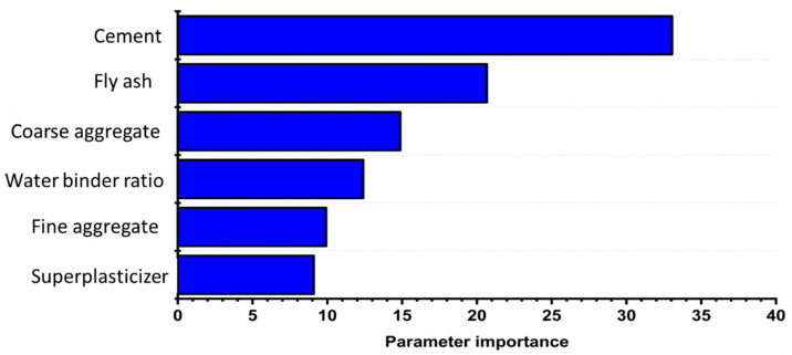
The influence of parameters on the compression strength of SCC was calculated by using machine learning (python) based program. It can be seen in Figure 6 that cement and fly ash play a vital role in SCC compressive strength prediction with 53% of their net contribution, whereas the coarse aggregate and water–binder ratio have an influence of 27.27% on the compressive strength of SCC.
Figure 6.
Features importance in strength prediction.
Development of the SCCs model incorporating waste material is based on the selection of input parameters. These variables have an intransigent impact on SCCs mechanical properties. All parameters in the dataset were carefully studied, and only the influential parameters for a generalized relationship were selected. The compressive strength response () of SCC depends upon the following factors as illustrated in Equation (1).
| (1) |
It must be noted that properly fitting parameters play an adamant part in the effectiveness and simplification of the established model. The factors for the GEP algorithm were calculated on the premise of research recommendations and numerous preliminary runs [62]. It must be kept in mind that gene chromosomes (population size) and head sizes are the key aspects in controlling program run time. Larger chromosome population and head size result in a longer time of test. Due to the number of possible results and the difficulty of the assessment model estimation, three best populations, i.e., 50, 100, or 150, and one head size were taken into consideration. The parameters for the model used in the GEP algorithm are listed in Table 5.
Table 5.
Gene expression programming variables detail set.
| Settings | |
| General property | |
| Chromosomes | 30 |
| Genes | 3, 4, 5 |
| Head size | 8 |
| Linking function | Multiplication |
| Function set | +, −, ×, ÷, exp |
| Numerical Constants | |
| Constant per gene | 10 |
| Data type | Floating number |
| Lower bound | −10 |
| Upper bound | 10 |
| Genetic Operators | |
| Mutation rate | 0.00138 |
| Inversion rate | 0.00546 |
| Insertion Sequences transposition rate | 0.00546 |
| Root Insertion Sequence transposition rate | 0.00546 |
| One-point recombination rate | 0.00277 |
| Two-point recombination rate | 0.00277 |
| Gene recombination rate | 0.00277 |
| Gene transposition rate | 0.00277 |
The correlation coefficient (R2) is a common mean degree of performance of any machine learning model. Nevertheless, the inconsiderateness of R to divide and multiply the productivity values into a constant implies that R (coefficient of relation) cannot be used exclusively as the predictive precision of any model. Therefore, errors such as the relative root mean square error (RMSE), mean absolute error (MAE), and relative mean square error (RSE) were also calculated. An output index or performance index (ρ) is proposed to measure model efficiency as a result of both R and RRMSE [63]. The calculated expressions are given as equations for these error functions, which are listed below:
| (2) |
| (3) |
| (4) |
where , , , and are experimental values setup and model domain.
5. Results and Discussion
5.1. Artificial Neural Network
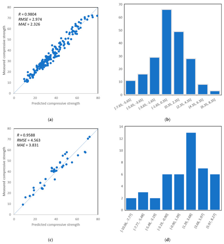
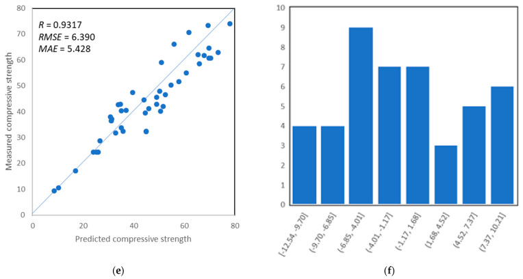
The influence of variables including regression coefficient R2 as well as statistical characteristics of errors between actual targets and modeled outputs are measured for the performance evaluation of the MLP-ANN model. The network output is assessed independently for training, validation, and testing set. The correlation between experimental values and prediction sets for training, validation, and testing set, respectively, are shown in Figure 7. It shows that the obstinate relation between an experimental set with modeled output for data exists. It can be seen that the training set, validation set, and test set give a coefficient of correlation close to 1, as illustrated in Figure 7a,c,e. Moreover, the prediction accuracy by ANN can also be evaluated by its error distribution. Figure 7b,d,f, present the error distribution of the training set, validation set, and testing set with prediction to output variables, showing satisfactory performance of the model. It can be seen that the error distribution of training set data between the experimentally measured compressive strength and predicted lies mostly below 10 MPa, showing that 93% of errors between the measured values and the predicted values lie in the range of 0 MPa to 10 MPa with error values between −7.65 MPa and 8.35 MPa, respectively, for training, as depicted in Figure 7b. Similarly, validation demonstrates the same trend by showing lesser error distribution in the same range of error values between −10.06 MPa and 8.27 MPa, as illustrated in Figure 7d, and for the testing set, the range of error values was a little bit higher and ranged between −12.54 MPa and 10.21 MPa, as depicted in Figure 7f. Thus, the prediction model shows obstinate and adamant modeling in relation to prediction and experimental results.
Figure 7.
(a) Predictions vs. target data of training set; (b) error distribution of ANN model with prediction versus training set; (c) predictions vs. target data of validation set; (d) error distribution of ANN model with prediction versus validation set; (e) predictions vs. target data of testing set; (f) error distribution of ANN model with prediction versus testing set.
5.2. Support Vector Machine
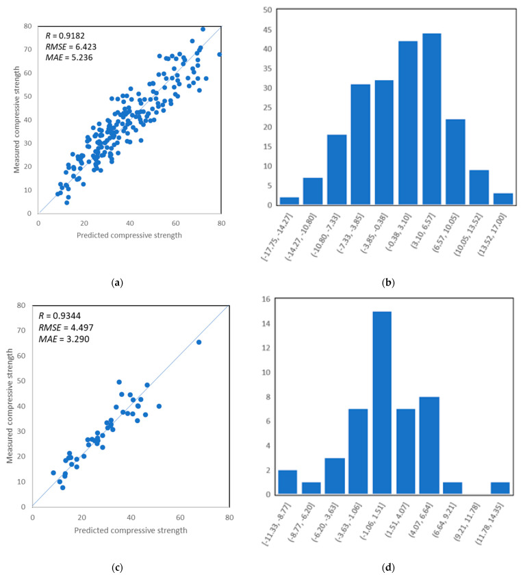
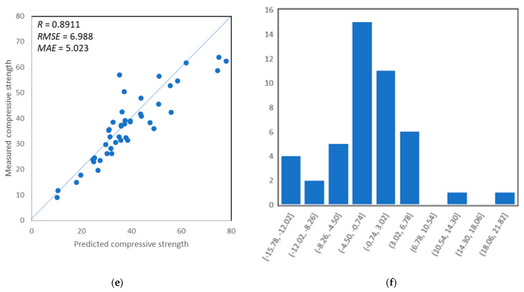
The influence of variables including regression coefficient R2 as well as statistical characteristics of errors between actual targets and modeled outputs are measured for the performance evaluation of the SVM model. The correlation between experimental values and prediction sets for training, validation, and testing set, respectively, are shown in Figure 8. It shows that the relation between an experimental set with modeled output for data exists, but it is not as sufficient as in comparison to ANN. It can be seen that training set, validation set, and test set give the coefficient of correlation are lower than for ANN but are still very high, as illustrated in Figure 8a,c,e. Moreover, the prediction accuracy by SVM is also illustrated by its error distribution, presented in Figure 8b,d,f). It can be seen that error values ranges between −17.75 MPa and 17.00 MPa, respectively, for training, as depicted in Figure 8b. Similarly, validation demonstrates the same trend by showing lesser error distribution in the same range of error values between −11.33 MPa and 14.35 MPa, as illustrated in Figure 8d, and for the testing set, the range of error values was a little bit higher and ranges between −15.78 MPa and 21.82 MPa, as depicted in Figure 8f. Thus, the prediction model shows less accuracy in comparison to ANN.
Figure 8.
(a) Predictions vs. target data of training set; (b) error distribution of SVM model with prediction versus training set; (c) predictions vs. target data of validation set; (d) error distribution of SVM model with prediction versus validation set; (e) predictions vs. target data of testing set; (f) error distribution of SVM model with prediction versus testing set.
5.3. Gene Expression Programming
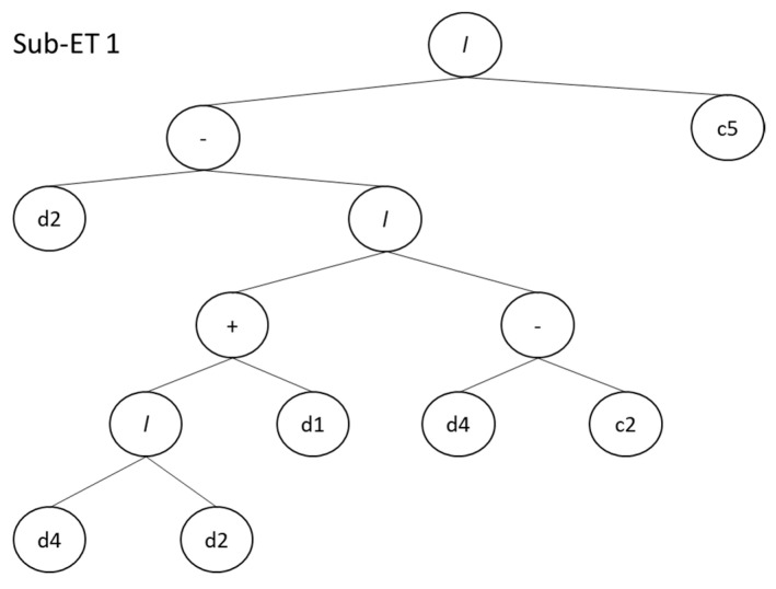
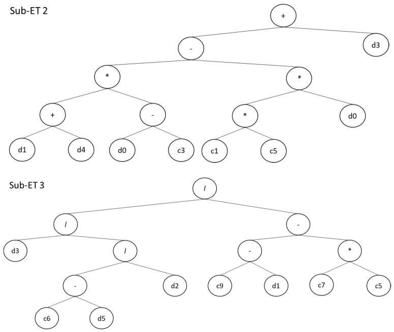
The output of the GEP algorithm for the SCC model is denoted as an expression tree(s), as illustrated in Figure 9. The GEP algorithm solves nonlinear expressions as well as linear ones by forming a tree-like structure, which can then be used to form an equation used to predict the model outcome. These ETs were then decoded to give empirical relationships. The ETs for compressive strength of SCC contains four basic mathematical functions containing addition, multiplication, subtraction, and division. Moreover, it can be seen that these expression trees contain parameters and constants to prepare empirical equations, as shown in Table 6.
Figure 9.
GEP model expression trees of SCC.
Table 6.
Constant and notation used to prepare empirical equation.
| Parameters Notation | Parameters | Constant Notations | Constant Values |
|---|---|---|---|
| d0 | Cement | G1C5 | −4.28835075 |
| d1 | Fly ash | G1C2 | 37.75001621 |
| d2 | Water–powder | G2C3 | 39.89209066 |
| d3 | Fine aggregate | G2C1 | 9.967413128 |
| d4 | Coarse aggregate | G2C5 | 26.22055325 |
| d5 | Superplasticizer | G3C9 | −20.52776364 |
| - | - | G3C7 | 145.5520044 |
| - | - | G3C5 | −10.5395382 |
| - | - | G3C6 | 544.4511609 |
Defined relationships between ETs and genes help in predicting the compressive properties of self-compacting concrete (). The response to predict the compressive strength is then proposed with expression trees by using Equation (5).
| (5) |
where:
| (6) |
| (7) |
| (8) |
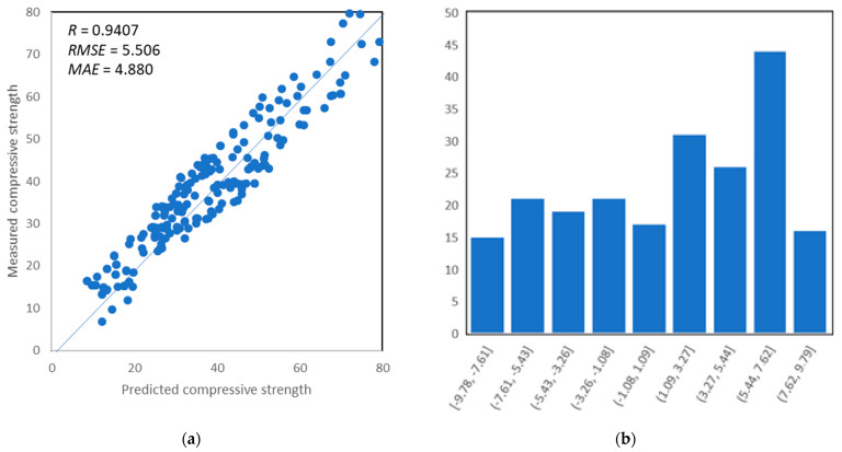
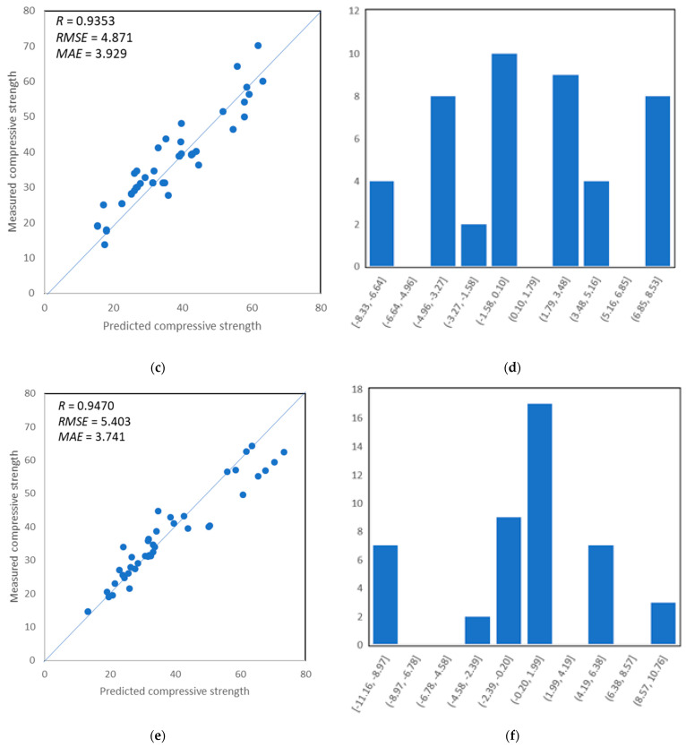
The evaluation of the model expectations against the actual results of SCC strength is graphically shown in Figure 10. It depicts that all input variables to predict f′c of SCC are accurately taken into account by the model. The presented results are highly correlated, as be seen in Figure 10a,c,e; it was also proved by the obtained values of linear correlation coefficient, equal to 0.941, 0.935, and 0.947 for training and validation. The proposed model’s efficiency is significantly affected by the number of datasets [63]. This research consists of 300 datasets in the prediction of SCC; hence, high accuracy of the model is expected. The response of predicted values with error distribution is presented in Figure 10b,d,f. It can be seen that all sets for the GEP model show a minimum error with the maximum range that lies below 10 MPa, as depicted in Figure 10b,d,f. It confirms the accuracy of the desired model with respect to regression models and it is on the same level of accuracy as for ANN.
Figure 10.
(a) Predictions vs. target data of training set; (b) error distribution of GEP model with prediction versus training set; (c) predictions vs. target data of validation set; (d) error distribution of GEP model with prediction versus validation set; (e) predictions vs. target data of testing set; (f) error distribution of GEP model with prediction versus testing set.
5.4. Comparison between the Proposed Models
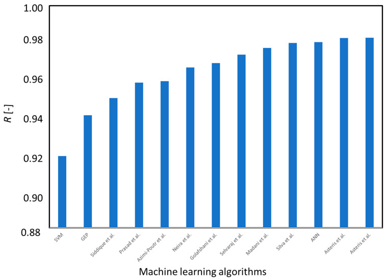
The machine learning algorithms used in the article are accurate in prediction of the compressive strength of self-compacting concrete modified by fly ash. It can be observed based on the values of the parameters describing their accuracy, which were linear coefficient of correlation R, root mean square error RMSE, and mean average error MAE. Among the artificial neural networks, the support vector machine and gene expression programming, there is difficult to point the most accurate algorithm. The least accurate was support vector machine due to the lowest values of the linear coefficient of correlation and the highest values of errors in all processes. However, even though the neural network was the most accurate during the training process, the gene expression programming algorithm was more accurate in the testing and validation processes. Thus, for construction practice, it might be beneficial to use this algorithm, which performs better in the testing and validation processes instead of training because of the threat of overfitting. In Figure 11, the aforementioned algorithms were compared with other models presented in the literature.
Figure 11.
The comparison of models for SCC compressive strength prediction.
It can be seen that all of the investigated models are predict the SCC compressive strength well, according to the literature. However, due to the fact that none of the models were perfectly accurate (linear correlation coefficient was equal to 1.0), it is still possible to improve the algorithms by building other databases or using different algorithms.
6. Conclusions
This research discusses the machine learning application of artificial intelligence, in particular, artificial neural network, support vector machine, and gene expression programming for the prediction of self-compacting concrete compressive strength. By performing an extensive literature survey for obtaining the experimental results of the SCCs compressive strength values and also by performing numerical analysis using ANN, SVM, and GEP, the following conclusions can be drawn:
ANN-, SVM-, and GEP-based models predict the properties of SCC strength; however, ANN and GEP are the most accurate for this purpose;
ANN, SVM, and GEP models were characterized by the very high values of linear correlation coefficient equal to R = 0.9588, R = 0.9344 and R = 0.9353 for the testing set, respectively. The test set of the ANN, SVM, and GEP models show average error values of 5.428 MPa, 5.023 MPa, and 3.741 MPa, respectively. This indicates that the GEP model was able to be performed better in terms of accuracy during this process in comparison to the ANN and SVM models;
Permutation features show clear influential parameters for strength prediction. Variable such as the ratio of cement and fly ash added to the mixture have a major effect on strength with 53% out of total parameters. Thus, it is important to know their ratio in the mixture in order to evaluate the SCC compressive strength; without this variable, the modelling might be less accurate;
Statistical analysis and external checks give obstinate responses for all models.
These models were used for prediction rather than conducting experimental work; thus, their utilization in the civil engineering field will lower the carbon footprint. Below, a few recommendations for continuing similar research in the future are presented:
Hybrid models or advanced evolutionary algorithms can be developed, and the results can be compared to the present study.
The techniques used in this study can be used to model other engineering properties of concrete and structures.
As every study and technique has some limitations, some of the limitations of GEP are as follows:
Sometimes, the GEP is trapped in a local region that does not contain the global optimum. This phenomenon is called premature convergence and is one of the serious problems in genetic algorithms.
The “best” fitness is in comparison to other fitness; i.e., the stop criterion is not clear in every problem.
For specific optimization problems and problem instances, other optimization algorithms may be more efficient than genetic algorithms in terms of speed of convergence.
Appendix A
Table A1.
Self-compacting concrete mixture components and compressive strength.
| No. | Cement | Fly Ash | Water–Powder Ratio | Sand | Coarse Aggregate | Superplasticizer | Strength |
|---|---|---|---|---|---|---|---|
| - | kg/m3 | kg/m3 | - | kg/m3 | kg/m3 | kg/m3 | MPa |
| 1 | 148 | 137 | 0.55 | 830 | 1002 | 0.11 | 17.95 |
| 2 | 393 | 0 | 0.49 | 758 | 940 | 0 | 39.58 |
| 3 | 325 | 60 | 0.65 | 900 | 850 | 0.12 | 31.4 |
| 4 | 374.3 | 0 | 0.51 | 730.4 | 1013.2 | 0.02 | 39.06 |
| 5 | 348 | 224 | 0.5 | 783 | 848 | 0.43 | 58.6 |
| 6 | 296 | 107 | 0.55 | 778 | 819 | 0.04 | 31.42 |
| 7 | 350 | 162 | 0.41 | 768 | 840 | 0.18 | 51.7 |
| 8 | 296 | 106.7 | 0.55 | 778.4 | 819.2 | 0.04 | 31.42 |
| 9 | 374 | 0 | 0.51 | 730 | 1013 | 0.02 | 39.05 |
| 10 | 148.1 | 136.6 | 0.56 | 830.1 | 1001.8 | 0.11 | 17.96 |
| 11 | 275 | 0 | 0.67 | 808 | 1088 | 0 | 24.5 |
| 12 | 231.75 | 121.62 | 0.49 | 778.45 | 1056.4 | 0.03 | 33.73 |
| 13 | 181.38 | 167.01 | 0.49 | 777.8 | 1055.6 | 0.04 | 27.77 |
| 14 | 194.68 | 100.52 | 0.56 | 905.9 | 1006.4 | 0.04 | 25.72 |
| 15 | 325 | 60 | 0.65 | 899 | 850 | 0.43 | 30.8 |
| 16 | 420 | 80 | 0.33 | 785 | 860 | 0.3 | 56 |
| 17 | 212.52 | 100.37 | 0.51 | 903.59 | 1007.8 | 0.04 | 31.64 |
| 18 | 290 | 100 | 0.33 | 913 | 837 | 0.01 | 42.7 |
| 19 | 333 | 0 | 0.58 | 842.6 | 931.2 | 0 | 31.97 |
| 20 | 250 | 160 | 0.55 | 742 | 837 | 0.5 | 28.5 |
| 21 | 339 | 0 | 0.58 | 781 | 968 | 0 | 32.04 |
| 22 | 207 | 207 | 0.45 | 845 | 843 | 0.4 | 33.2 |
| 23 | 252 | 0 | 0.73 | 784 | 1111 | 0 | 19.69 |
| 24 | 360 | 240 | 0.28 | 853 | 698 | 0.3 | 63.5 |
| 25 | 417 | 153 | 0.32 | 828 | 759 | 0.31 | 61.82 |
| 26 | 163 | 245 | 0.4 | 851 | 851 | 0.2 | 26.2 |
| 27 | 310 | 0 | 0.62 | 850 | 970 | 0 | 27.92 |
| 28 | 350 | 133 | 0.38 | 815 | 883 | 0.34 | 55.3 |
| 29 | 190.34 | 125.18 | 0.51 | 802.59 | 1088.1 | 0.05 | 28.47 |
| 30 | 427 | 115 | 0.36 | 779 | 844 | 0.26 | 59.4 |
| 31 | 475 | 0 | 0.48 | 594 | 932 | 0 | 39.29 |
| 32 | 164.6 | 150.4 | 0.58 | 728.9 | 1023.3 | 0.07 | 18.03 |
| 33 | 165 | 150 | 0.58 | 729 | 1023 | 0.07 | 18.03 |
| 34 | 318 | 126 | 0.47 | 737 | 861 | 0.02 | 40.06 |
| 35 | 317.9 | 126.5 | 0.47 | 736.6 | 860.5 | 0.02 | 40.06 |
| 36 | 280 | 96 | 0.87 | 817 | 850 | 0.62 | 15.9 |
| 37 | 540 | 0 | 0.32 | 613 | 1125 | 0 | 67.31 |
| 38 | 183 | 160 | 0.55 | 891 | 837 | 0.5 | 22.1 |
| 39 | 238.05 | 94.11 | 0.56 | 847.01 | 949.91 | 0.03 | 30.23 |
| 40 | 307 | 0 | 0.63 | 812 | 968 | 0 | 27.53 |
| 41 | 480 | 96 | 0.38 | 819 | 699 | 0.94 | 53 |
| 42 | 144.8 | 133.6 | 0.65 | 811.5 | 979.5 | 0.08 | 13.2 |
| 43 | 145 | 134 | 0.65 | 812 | 979 | 0.08 | 13.2 |
| 44 | 151.6 | 111.9 | 0.7 | 815.9 | 992 | 0.05 | 12.18 |
| 45 | 325 | 60 | 0.85 | 722 | 850 | 0.43 | 13.3 |
| 46 | 370 | 24 | 0.69 | 772 | 850 | 0.25 | 26.4 |
| 47 | 152 | 112 | 0.7 | 816 | 992 | 0.05 | 12.18 |
| 48 | 331 | 0 | 0.58 | 825 | 978 | 0 | 31.45 |
| 49 | 252.5 | 0 | 0.74 | 784.3 | 1111.6 | 0 | 19.77 |
| 50 | 505 | 60 | 0.35 | 630 | 1030 | 0 | 64.02 |
| 51 | 134.7 | 165.7 | 0.6 | 804.9 | 961 | 0.07 | 13.29 |
| 52 | 325 | 60 | 0.65 | 899 | 850 | 0.43 | 32.6 |
| 53 | 135 | 166 | 0.6 | 805 | 961 | 0.07 | 13.29 |
| 54 | 475 | 0 | 0.34 | 662 | 1044 | 0.02 | 58.52 |
| 55 | 251.37 | 118.27 | 0.52 | 754.3 | 1043.6 | 0.02 | 33.27 |
| 56 | 166.09 | 163.27 | 0.54 | 780.09 | 1058.6 | 0.03 | 21.54 |
| 57 | 393 | 0 | 0.49 | 785.6 | 940.6 | 0 | 39.6 |
| 58 | 250 | 0 | 0.73 | 820 | 1100 | 0 | 20.87 |
| 59 | 210 | 100 | 0.65 | 910 | 837 | 0.8 | 19.1 |
| 60 | 190.68 | 125.4 | 0.51 | 804.01 | 1090 | 0.04 | 26.4 |
| 61 | 249 | 60 | 0.68 | 1079 | 850 | 0.43 | 24 |
| 62 | 405 | 0 | 0.43 | 695 | 1120 | 0 | 52.3 |
| 63 | 528 | 0 | 0.35 | 720 | 920 | 0.01 | 56.83 |
| 64 | 250 | 160 | 0.55 | 739 | 837 | 0 | 27.3 |
| 65 | 273 | 90 | 0.55 | 762 | 931 | 0.04 | 32.24 |
| 66 | 297.16 | 117.54 | 0.42 | 753.45 | 1022.8 | 0.03 | 47.4 |
| 67 | 169 | 254 | 0.45 | 853 | 853 | 0 | 30.2 |
| 68 | 272.6 | 89.6 | 0.55 | 762.2 | 931.3 | 0.04 | 32.25 |
| 69 | 190.34 | 125.18 | 0.53 | 798.9 | 1079 | 0.05 | 24.85 |
| 70 | 310 | 0 | 0.62 | 830 | 1012 | 0 | 27.83 |
| 71 | 298 | 107 | 0.52 | 744 | 880 | 0.04 | 31.87 |
| 72 | 298.2 | 107 | 0.52 | 744.2 | 879.6 | 0.04 | 31.88 |
| 73 | 251.37 | 118.27 | 0.51 | 757.73 | 1028.4 | 0.03 | 32.66 |
| 74 | 247 | 165 | 0.45 | 845 | 846 | 0.12 | 34.6 |
| 75 | 400 | 0 | 0.47 | 745 | 1025 | 0 | 43.7 |
| 76 | 170 | 200 | 0.43 | 930 | 900 | 0.2 | 31 |
| 77 | 289 | 0 | 0.66 | 895.3 | 913.2 | 0 | 25.57 |
| 78 | 317 | 160 | 0.55 | 594 | 837 | 0.5 | 29.1 |
| 79 | 326 | 138 | 0.43 | 792 | 801 | 0.03 | 40.68 |
| 80 | 295 | 0 | 0.63 | 769 | 1069 | 0 | 25.18 |
| 81 | 520 | 0 | 0.33 | 855 | 855 | 0.01 | 60.28 |
| 82 | 225 | 275 | 0.35 | 908 | 652 | 0.7 | 41.42 |
| 83 | 222.36 | 96.67 | 0.59 | 870.32 | 967.08 | 0.02 | 24.89 |
| 84 | 165 | 143.57 | 0.53 | 900.9 | 1005.6 | 0 | 26.2 |
| 85 | 238 | 0 | 0.78 | 789 | 1119 | 0 | 17.54 |
| 86 | 238 | 0 | 0.78 | 789 | 1118 | 0 | 17.54 |
| 87 | 238.1 | 0 | 0.78 | 789.3 | 1118.8 | 0 | 17.58 |
| 88 | 238 | 159 | 0.4 | 844 | 844 | 0.29 | 37.8 |
| 89 | 522 | 0 | 0.28 | 896 | 896 | 0 | 74.99 |
| 90 | 148 | 182 | 0.55 | 884 | 839 | 0.1 | 15.52 |
| 91 | 290 | 100 | 0.65 | 709 | 837 | 0.2 | 26.6 |
| 92 | 148.1 | 182.1 | 0.55 | 884.3 | 838.9 | 0.1 | 15.53 |
| 93 | 154.8 | 142.8 | 0.65 | 696.7 | 1047.4 | 0.06 | 12.46 |
| 94 | 302 | 0 | 0.67 | 817 | 974 | 0 | 21.75 |
| 95 | 155 | 143 | 0.65 | 697 | 1047 | 0.06 | 12.46 |
| 96 | 280 | 120 | 0.39 | 946 | 900 | 0.35 | 45 |
| 97 | 255 | 0 | 0.75 | 945 | 889.8 | 0 | 18.75 |
| 98 | 250 | 160 | 0.55 | 746 | 837 | 1 | 26.7 |
| 99 | 400 | 60 | 0.63 | 718 | 850 | 0.43 | 30.4 |
| 100 | 322 | 0 | 0.63 | 800 | 974 | 0 | 25.18 |
| 101 | 250 | 160 | 0.55 | 742 | 837 | 0.5 | 26.4 |
| 102 | 220 | 180 | 0.45 | 850 | 900 | 0.35 | 38 |
| 103 | 350 | 90 | 0.48 | 852 | 923 | 0.14 | 46.5 |
| 104 | 290 | 100 | 0.45 | 913 | 837 | 0.8 | 42.7 |
| 105 | 213.74 | 174.74 | 0.4 | 776.35 | 1053.5 | 0.05 | 40.15 |
| 106 | 331 | 0 | 0.58 | 821 | 1025 | 0 | 31.74 |
| 107 | 427 | 115 | 0.45 | 779 | 844 | 0.12 | 59.4 |
| 108 | 295.8 | 0 | 0.63 | 769.3 | 1091.4 | 0 | 25.22 |
| 109 | 281 | 0 | 0.66 | 774 | 1104 | 0 | 22.44 |
| 110 | 281 | 0 | 0.66 | 774 | 1104 | 0 | 22.44 |
| 111 | 296 | 0 | 0.63 | 769 | 1090 | 0 | 25.18 |
| 112 | 325 | 60 | 0.65 | 898 | 850 | 0.43 | 34.3 |
| 113 | 250 | 160 | 0.55 | 742 | 837 | 0.5 | 26 |
| 114 | 275 | 275 | 0.37 | 796 | 937 | 0.74 | 63.32 |
| 115 | 300 | 0 | 0.61 | 795 | 1075 | 0 | 26.85 |
| 116 | 298.1 | 107 | 0.46 | 815.2 | 879 | 0.02 | 42.64 |
| 117 | 298 | 107 | 0.46 | 815 | 879 | 0.02 | 42.64 |
| 118 | 290 | 100 | 0.48 | 709 | 837 | 0 | 26.6 |
| 119 | 325 | 60 | 0.65 | 896 | 850 | 0.75 | 27.7 |
| 120 | 220 | 180 | 0.39 | 916 | 900 | 0.6 | 43 |
| 121 | 370 | 96 | 0.57 | 833 | 850 | 0.25 | 39.5 |
| 122 | 225 | 0 | 0.8 | 833 | 1113 | 0 | 17.34 |
| 123 | 200 | 200 | 0.4 | 842 | 843 | 0.17 | 34.9 |
| 124 | 143.6 | 174.9 | 0.5 | 844.5 | 942.7 | 0.12 | 15.42 |
| 125 | 250 | 95.69 | 0.54 | 861.17 | 956.86 | 0.02 | 29.22 |
| 126 | 144 | 175 | 0.5 | 844 | 943 | 0.13 | 15.42 |
| 127 | 322 | 138 | 0.35 | 693.81 | 1085.2 | 0 | 58 |
| 128 | 322.5 | 107.5 | 0.47 | 1135 | 630 | 0.01 | 43.98 |
| 129 | 325 | 60 | 0.65 | 898 | 850 | 0.43 | 35 |
| 130 | 250 | 160 | 0.55 | 742 | 837 | 0.5 | 25.3 |
| 131 | 212.07 | 121.62 | 0.54 | 779.32 | 1057.6 | 0.03 | 24.9 |
| 132 | 301 | 129 | 0.47 | 1135 | 630 | 0.01 | 44 |
| 133 | 325 | 0 | 0.57 | 783 | 1063 | 0 | 30.57 |
| 134 | 218.85 | 124.13 | 0.46 | 794.91 | 1078.7 | 0.05 | 30.22 |
| 135 | 325 | 60 | 0.65 | 899 | 850 | 0.43 | 35.3 |
| 136 | 370 | 96 | 0.57 | 830 | 850 | 0.62 | 38.8 |
| 137 | 170 | 200 | 0.43 | 928 | 900 | 0.5 | 33 |
| 138 | 330 | 220 | 0.32 | 700 | 899 | 0.69 | 60.9 |
| 139 | 375 | 0 | 0.5 | 758 | 1038 | 0 | 38.21 |
| 140 | 275 | 250 | 0.35 | 775 | 840 | 0.2 | 54.5 |
| 141 | 399 | 100 | 0.35 | 814 | 882 | 0.15 | 55 |
| 142 | 339 | 0 | 0.55 | 754 | 1060 | 0 | 31.65 |
| 143 | 233.81 | 94.58 | 0.6 | 852.16 | 947.04 | 0.02 | 22.84 |
| 144 | 326.5 | 137.9 | 0.43 | 792.5 | 801.1 | 0.03 | 38.63 |
| 145 | 210 | 220 | 0.45 | 768 | 837 | 0.8 | 26.7 |
| 146 | 277 | 0 | 0.69 | 856 | 968 | 0 | 25.97 |
| 147 | 350 | 0 | 0.53 | 770 | 1050 | 0 | 34.29 |
| 148 | 339.2 | 0 | 0.55 | 754.3 | 1069.2 | 0 | 31.9 |
| 149 | 339 | 0 | 0.55 | 754 | 1069 | 0 | 31.84 |
| 150 | 220 | 180 | 0.39 | 916 | 900 | 0.1 | 44 |
| 151 | 280 | 96 | 0.87 | 820 | 850 | 0.25 | 19.6 |
| 152 | 350 | 150 | 0.35 | 900 | 600 | 1 | 37.18 |
| 153 | 229.68 | 118.16 | 0.56 | 757.63 | 1028.1 | 0.03 | 24.54 |
| 154 | 237 | 133 | 0.36 | 1034 | 900 | 0.2 | 49 |
| 155 | 258 | 172 | 0.47 | 1135 | 630 | 0.01 | 43.18 |
| 156 | 150.9 | 183.9 | 0.5 | 772.2 | 991.2 | 0.08 | 15.57 |
| 157 | 295.71 | 95.64 | 0.44 | 859.2 | 955.14 | 0.03 | 39.94 |
| 158 | 151 | 184 | 0.5 | 772 | 991 | 0.08 | 15.57 |
| 159 | 300 | 300 | 0.28 | 787 | 720 | 0.33 | 52.7 |
| 160 | 220 | 330 | 0.32 | 686 | 881 | 0.62 | 47.5 |
| 161 | 250 | 95.69 | 0.55 | 857.2 | 948.9 | 0.02 | 27.22 |
| 162 | 275 | 155 | 0.43 | 827 | 900 | 0.5 | 48 |
| 163 | 277.05 | 97.39 | 0.43 | 875.61 | 973.9 | 0.04 | 48.28 |
| 164 | 229.97 | 118.31 | 0.56 | 758.59 | 1029.4 | 0.02 | 24.48 |
| 165 | 165 | 385 | 0.34 | 656 | 834 | 1 | 34.9 |
| 166 | 145 | 179 | 0.62 | 869 | 824 | 0.06 | 10.54 |
| 167 | 327 | 173 | 0.35 | 902 | 803 | 0.41 | 61.6 |
| 168 | 279.5 | 150.5 | 0.47 | 1135 | 630 | 0.01 | 44.34 |
| 169 | 145.4 | 178.9 | 0.62 | 868.7 | 824 | 0.05 | 10.54 |
| 170 | 83 | 468 | 0.41 | 624 | 794 | 1 | 14.64 |
| 171 | 325 | 325 | 0.34 | 611 | 777 | 1.18 | 50.07 |
| 172 | 376 | 0 | 0.57 | 762.36 | 1003.5 | 0 | 31.97 |
| 173 | 251.37 | 118.27 | 0.51 | 757.73 | 1028.4 | 0.02 | 29.65 |
| 174 | 250 | 160 | 0.55 | 742 | 837 | 0.5 | 24.1 |
| 175 | 250 | 160 | 0.38 | 919 | 837 | 0.5 | 36.3 |
| 176 | 290 | 220 | 0.45 | 625 | 837 | 0.2 | 32.9 |
| 177 | 296 | 0 | 0.65 | 765 | 1085 | 0 | 21.65 |
| 178 | 428 | 257 | 0.27 | 788 | 736 | 0.02 | 74.5 |
| 179 | 250 | 257 | 0.38 | 787 | 853 | 0.23 | 51.5 |
| 180 | 350 | 0 | 0.58 | 775 | 974 | 0 | 27.34 |
| 181 | 200 | 0 | 0.9 | 845 | 1125 | 0 | 12.25 |
| 182 | 183 | 160 | 0.29 | 891 | 837 | 0.01 | 22.1 |
| 183 | 220 | 180 | 0.39 | 916 | 900 | 0.35 | 45 |
| 184 | 212 | 124.78 | 0.47 | 799.54 | 1085.4 | 0.04 | 38.5 |
| 185 | 250 | 160 | 0.34 | 742 | 837 | 0.01 | 28.5 |
| 186 | 500 | 0 | 0.28 | 853 | 966 | 0.01 | 67.57 |
| 187 | 325 | 120 | 0.75 | 755 | 850 | 0.43 | 32.2 |
| 188 | 154.8 | 142.8 | 0.65 | 867.7 | 877.2 | 0.06 | 9.74 |
| 189 | 155 | 143 | 0.65 | 868 | 877 | 0.06 | 9.74 |
| 190 | 500 | 101 | 0.32 | 820 | 753 | 0.38 | 70.93 |
| 191 | 382 | 0 | 0.49 | 739 | 1047 | 0 | 37.42 |
| 192 | 150.7 | 185.3 | 0.5 | 678 | 1074.5 | 0.1 | 13.46 |
| 193 | 382.5 | 0 | 0.49 | 739.3 | 1047.8 | 0 | 37.44 |
| 194 | 151 | 185 | 0.5 | 678 | 1074 | 0.11 | 13.46 |
| 195 | 225 | 525 | 0.33 | 487 | 620 | 1.36 | 34.83 |
| 196 | 275.07 | 121.35 | 0.4 | 777.5 | 1053.6 | 0.04 | 51.33 |
| 197 | 349 | 0 | 0.55 | 809 | 1056 | 0 | 33.61 |
| 198 | 313 | 113 | 0.42 | 689 | 1002 | 0.03 | 36.8 |
| 199 | 313.3 | 113 | 0.42 | 688.7 | 1001.9 | 0.03 | 36.8 |
| 200 | 348 | 224 | 0.31 | 783 | 848 | 0.9 | 58.6 |
| 201 | 420 | 180 | 0.32 | 900 | 750 | 0.03 | 79.19 |
| 202 | 276 | 184 | 0.35 | 693.81 | 1085.2 | 0 | 56 |
| 203 | 385 | 136 | 0.3 | 768 | 903 | 0.05 | 55.55 |
| 204 | 382 | 0 | 0.48 | 739 | 1047 | 0 | 37.42 |
| 205 | 440 | 110 | 0.32 | 714 | 917 | 0.69 | 69.8 |
| 206 | 349 | 162 | 0.39 | 779 | 852 | 0.29 | 59.9 |
| 207 | 349 | 0 | 0.55 | 806 | 1047 | 0 | 32.72 |
| 208 | 477 | 53 | 0.45 | 768 | 668 | 0.09 | 32.19 |
| 209 | 212.57 | 100.39 | 0.51 | 903.79 | 1003.8 | 0.05 | 37.4 |
| 210 | 325 | 0 | 0.55 | 1042 | 850 | 0.43 | 41.2 |
| 211 | 397 | 0 | 0.47 | 734 | 1040 | 0 | 39.09 |
| 212 | 250 | 160 | 0.72 | 566 | 837 | 0.5 | 11 |
| 213 | 370 | 24 | 0.69 | 770 | 850 | 0.62 | 18.7 |
| 214 | 236 | 0 | 0.82 | 885 | 968 | 0 | 18.42 |
| 215 | 250 | 160 | 0.34 | 739 | 837 | 0 | 27.3 |
| 216 | 197 | 197 | 0.35 | 856 | 856 | 0.28 | 38.9 |
| 217 | 237 | 133 | 0.43 | 960 | 900 | 0.5 | 46 |
| 218 | 350 | 133 | 0.52 | 815 | 883 | 0.16 | 55.3 |
| 219 | 165 | 385 | 0.58 | 735 | 865 | 0.84 | 37.92 |
| 220 | 312.7 | 0 | 0.57 | 822.2 | 999.7 | 0.03 | 25.1 |
| 221 | 317 | 160 | 0.37 | 594 | 837 | 0.01 | 29.1 |
| 222 | 313 | 0 | 0.57 | 822 | 1000 | 0.03 | 25.1 |
| 223 | 350 | 90 | 0.39 | 852 | 923 | 0.3 | 46.5 |
| 224 | 313.8 | 112.6 | 0.4 | 782.9 | 925.3 | 0.03 | 38.46 |
| 225 | 380 | 20 | 0.38 | 1180 | 578 | 0.4 | 40.4 |
| 226 | 407 | 244 | 0.28 | 815 | 761 | 0.02 | 70.4 |
| 227 | 314 | 113 | 0.4 | 783 | 925 | 0.03 | 38.46 |
| 228 | 248 | 203 | 0.39 | 808 | 900 | 0.35 | 50 |
| 229 | 304.8 | 99.6 | 0.48 | 705.2 | 959.4 | 0.03 | 30.12 |
| 230 | 305 | 100 | 0.48 | 705 | 959 | 0.03 | 30.12 |
| 231 | 480 | 0 | 0.4 | 712.2 | 936.2 | 0 | 43.94 |
| 232 | 220 | 180 | 0.33 | 982 | 900 | 0.35 | 51 |
| 233 | 164 | 200 | 0.5 | 846 | 849 | 0.08 | 15.09 |
| 234 | 210 | 100 | 0.44 | 910 | 837 | 0.01 | 19.1 |
| 235 | 344 | 147 | 0.35 | 814 | 881 | 0.12 | 48.75 |
| 236 | 164.2 | 200.1 | 0.5 | 846 | 849.3 | 0.08 | 15.09 |
| 237 | 357 | 193 | 0.33 | 878 | 742 | 0.02 | 67.5 |
| 238 | 275 | 155 | 0.43 | 830 | 900 | 0.2 | 36 |
| 239 | 333 | 215 | 0.33 | 835 | 766 | 0.24 | 50.24 |
| 240 | 220 | 180 | 0.39 | 916 | 900 | 0.35 | 47 |
| 241 | 250 | 160 | 0.34 | 746 | 837 | 0.01 | 26.7 |
| 242 | 321 | 128 | 0.41 | 780 | 870 | 0.03 | 37.26 |
| 243 | 321.4 | 127.9 | 0.41 | 779.7 | 870.1 | 0.04 | 37.27 |
| 244 | 250 | 160 | 0.23 | 919 | 837 | 0.01 | 36.3 |
| 245 | 250 | 160 | 0.34 | 742 | 837 | 0.01 | 26.4 |
| 246 | 355.9 | 141.6 | 0.39 | 778.4 | 801.4 | 0.03 | 40.87 |
| 247 | 356 | 142 | 0.39 | 778 | 801 | 0.03 | 40.87 |
| 248 | 460 | 0 | 0.35 | 693.81 | 1085.2 | 0 | 68 |
| 249 | 298 | 107 | 0.4 | 784 | 953 | 0.04 | 35.86 |
| 250 | 350 | 111 | 0.39 | 831 | 900 | 0.32 | 61 |
| 251 | 485 | 0 | 0.3 | 800 | 1120 | 0 | 71.99 |
| 252 | 298.1 | 107.5 | 0.4 | 784 | 953.2 | 0.04 | 35.87 |
| 253 | 480 | 0 | 0.4 | 721 | 936 | 0 | 43.89 |
| 254 | 198 | 232 | 0.34 | 874 | 900 | 0.2 | 46 |
| 255 | 158 | 195 | 0.62 | 713 | 898 | 0.07 | 8.54 |
| 256 | 350 | 162 | 0.59 | 768 | 840 | 0.09 | 51.7 |
| 257 | 158.4 | 194.9 | 0.62 | 712.9 | 897.7 | 0.07 | 8.54 |
| 258 | 251.81 | 99.94 | 0.42 | 899.76 | 1006 | 0.05 | 33.94 |
| 259 | 249.1 | 98.75 | 0.45 | 889.01 | 987.76 | 0.05 | 30.85 |
| 260 | 210 | 220 | 0.22 | 786 | 837 | 0.01 | 26.7 |
| 261 | 275 | 275 | 0.34 | 691 | 880 | 1.25 | 57.9 |
| 262 | 250 | 160 | 0.34 | 742 | 837 | 0.01 | 26 |
| 263 | 250 | 261 | 0.55 | 478 | 837 | 0.5 | 17 |
| 264 | 161 | 241 | 0.35 | 866 | 864 | 0.3 | 35.8 |
| 265 | 300 | 200 | 0.35 | 923 | 663 | 0.7 | 54.69 |
| 266 | 540 | 0 | 0.3 | 676 | 1055 | 0 | 61.89 |
| 267 | 290 | 220 | 0.26 | 625 | 837 | 0 | 32.9 |
| 268 | 525 | 0 | 0.36 | 613 | 1125 | 0 | 55.94 |
| 269 | 213.5 | 174.24 | 0.41 | 771.9 | 1043.6 | 0.05 | 44.64 |
| 270 | 465 | 85 | 0.41 | 910 | 590 | 0.02 | 35.19 |
| 271 | 250 | 275 | 0.34 | 842 | 772 | 0.23 | 39.62 |
| 272 | 210 | 220 | 0.65 | 562 | 837 | 0.2 | 10.2 |
| 273 | 397 | 0 | 0.47 | 734 | 1040 | 0 | 36.94 |
| 274 | 368 | 92 | 0.35 | 693.81 | 1085.2 | 0 | 66 |
| 275 | 465 | 85 | 0.41 | 910 | 590 | 0.97 | 35.19 |
| 276 | 250 | 160 | 0.34 | 742 | 837 | 0.01 | 25.3 |
| 277 | 520 | 0 | 0.34 | 805 | 870 | 0.01 | 51.02 |
| 278 | 213.5 | 174.24 | 0.4 | 775.48 | 1052.3 | 0.05 | 45.94 |
| 279 | 193 | 158 | 0.39 | 1024 | 900 | 0.35 | 44 |
| 280 | 437 | 80 | 0.34 | 743 | 924 | 0.43 | 69.7 |
| 281 | 500 | 0 | 0.3 | 655 | 1033 | 0.02 | 69.84 |
| 282 | 336.5 | 0 | 0.54 | 816.8 | 985.8 | 0.01 | 44.87 |
| 283 | 336 | 0 | 0.54 | 817 | 986 | 0.01 | 44.86 |
| 284 | 220 | 180 | 0.39 | 916 | 900 | 0.35 | 49 |
| 285 | 246.83 | 125.08 | 0.39 | 800.89 | 1086.8 | 0.05 | 52.5 |
| 286 | 220 | 180 | 0.39 | 916 | 900 | 0.12 | 49 |
| 287 | 385 | 0 | 0.48 | 763 | 966 | 0 | 31.35 |
| 288 | 540 | 60 | 0.33 | 900 | 750 | 0.02 | 78.05 |
| 289 | 322.2 | 115.6 | 0.45 | 813.4 | 817.9 | 0.03 | 31.18 |
| 290 | 322 | 116 | 0.45 | 813 | 818 | 0.03 | 31.18 |
| 291 | 250 | 160 | 0.34 | 742 | 837 | 0.01 | 24.1 |
| 292 | 290.35 | 96.18 | 0.43 | 865 | 961.18 | 0.03 | 34.74 |
| 293 | 252.31 | 98.75 | 0.42 | 889.01 | 987.76 | 0.06 | 50.6 |
| 294 | 380 | 145 | 0.35 | 988 | 659 | 0.28 | 65.5 |
| 295 | 344 | 86 | 0.47 | 1135 | 630 | 0.01 | 50.37 |
| 296 | 438 | 263 | 0.27 | 774 | 723 | 0.02 | 69.5 |
| 297 | 380 | 192 | 0.35 | 931 | 621 | 0.21 | 67.8 |
| 298 | 412 | 138 | 0.33 | 887 | 752 | 0.02 | 73.4 |
| 299 | 350 | 186 | 0.33 | 786 | 851 | 0.22 | 70.4 |
| 300 | 375 | 125 | 0.35 | 938 | 673 | 0.7 | 60.8 |
Author Contributions
Conceptualization, F.F., S.C., P.N., F.A., H.A. and K.A.O.; Data curation, F.F. and T.N.; Formal analysis, F.F. and T.N.; Funding acquisition, S.C. and K.A.O.; Investigation, S.C., P.N., F.A., H.A., K.Ś.-W. and S.M.; Methodology, F.F., S.C., P.N., F.A., H.A. and K.A.O.; Software, F.F., S.C., T.N. and S.M.; Supervision, K.A.O.; Visualization, K.Ś.-W. and S.M.; Writing–original draft, F.F., S.C., P.N., F.A., K.Ś.-W., T.N. and S.M.; Writing–review & editing, S.C., H.A. and K.A.O. All authors have read and agreed to the published version of the manuscript.
Funding
The APC was funded by Cracow University of Technology.
Institutional Review Board Statement
Not applicable.
Informed Consent Statement
Not applicable.
Data Availability Statement
All the data is available within the manuscript.
Conflicts of Interest
The authors declare no conflict of interest.
Footnotes
Publisher’s Note: MDPI stays neutral with regard to jurisdictional claims in published maps and institutional affiliations.
References
- 1.Zongjin L. Advanced Concrete Technology. 1st ed. John Wiley and Sons Ltd.; Hoboken, NJ, USA: 2011. pp. 1–521. [Google Scholar]
- 2.De Schutter G., Bartos P., Domone P., Gibbs J. Self-Compacting Concrete. Whittles Publishing; Caithness, UK: CRC Press, Taylor & Francis Group; Boca Raton, FL, USA: 2008. [Google Scholar]
- 3.Guru Jawahar J., Sashidhar C., Ramana Reddy I.V., Annie Peter J. Effect of coarse aggregate blending on short-term mechanical properties of self compacting concrete. Mater. Des. 2013;43:185–194. doi: 10.1016/j.matdes.2012.06.063. [DOI] [Google Scholar]
- 4.Li H., Yin J., Yan P., Sun H., Wan Q. Experimental Investigation on the Mechanical Properties of Self-Compacting Concrete under Uniaxial and Triaxial Stress. Materials. 2020;13:1830. doi: 10.3390/ma13081830. [DOI] [PMC free article] [PubMed] [Google Scholar]
- 5.Zhang X., Luo Y., Wang L., Zhang J., Wu W., Yang C. Flexural strengthening of damaged RC T-beams using self-compacting concrete jacketing under different sustaining load. Constr. Build. Mater. 2018;172:185–195. doi: 10.1016/j.conbuildmat.2018.03.245. [DOI] [Google Scholar]
- 6.Chalioris C.E., Pourzitidis C.N. Rehabilitation of Shear-Damaged Reinforced Concrete Beams Using Self-Compacting Concrete Jacketing. ISRN Civ. Eng. 2012;2012:816107. doi: 10.5402/2012/816107. [DOI] [Google Scholar]
- 7.Sucharda O., Brozovsky J., Mikolasek D. Numerical modelling and bearing capacity of reinforced concrete beams. Key Eng. Mater. 2014;577–578:281–284. doi: 10.4028/www.scientific.net/KEM.577-578.281. [DOI] [Google Scholar]
- 8.Czarnecki S., Shariq M., Nikoo M., Sadowski Ł. An intelligent model for the prediction of the compressive strength of cementitious composites with ground granulated blast furnace slag based on ultrasonic pulse velocity measurements. Meas. J. Int. Meas. Confed. 2021;172:108951. doi: 10.1016/j.measurement.2020.108951. [DOI] [Google Scholar]
- 9.Nicoara A.I., Stoica A.E., Vrabec M., Šmuc Rogan N., Sturm S., Ow-Yang C., Vasile B.S. End-of-life materials used as supplementary cementitious materials in the concrete industry. Materials. 2020;13:1954. doi: 10.3390/ma13081954. [DOI] [PMC free article] [PubMed] [Google Scholar]
- 10.EN British Standard . 450-1, Fly Ash for Concrete—Definition, Specifications and Conformity Criteria. British Standards Institution; London, UK: 2012. [Google Scholar]
- 11.Golewski G.L. Green concrete composite incorporating fly ash with high strength and fracture toughness. J. Clean. Prod. 2018;172:218–226. doi: 10.1016/j.jclepro.2017.10.065. [DOI] [Google Scholar]
- 12.Farooq F., Rahman S.K.U., Akbar A., Khushnood R.A., Javed M.F., Alyousef R., Alabduljabbar H., Aslam F. A comparative study on performance evaluation of hybrid GNPs/CNTs in conventional and self-compacting mortar. Alex. Eng. J. 2020;59:369–379. doi: 10.1016/j.aej.2019.12.048. [DOI] [Google Scholar]
- 13.Bušić R., Benšić M., Miličević I., Strukar K. Prediction models for the mechanical properties of self-compacting concrete with recycled rubber and silica fume. Materials. 2020;13:1821. doi: 10.3390/ma13081821. [DOI] [PMC free article] [PubMed] [Google Scholar]
- 14.Deifalla A.F., Zapris A.G., Chalioris C.E. Multivariable Regression Strength Model for Steel Fiber-Reinforced Concrete Beams under Torsion. Materials. 2021;14:3889. doi: 10.3390/ma14143889. [DOI] [PMC free article] [PubMed] [Google Scholar]
- 15.Sucharda O., Pajak M., Ponikiewski T., Konecny P. Identification of mechanical and fracture properties of self-compacting concrete beams with different types of steel fibres using inverse analysis. Constr. Build. Mater. 2017;138:263–275. doi: 10.1016/j.conbuildmat.2017.01.077. [DOI] [Google Scholar]
- 16.Asteris P.G., Kolovos K.G., Douvika M.G., Roinos K. Prediction of self-compacting concrete strength using artificial neural networks. Eur. J. Environ. Civ. Eng. 2016;20:102–122. doi: 10.1080/19648189.2016.1246693. [DOI] [Google Scholar]
- 17.Asteris P.G., Kolovos K.G. Self-compacting concrete strength prediction using surrogate models. Neural Comput. Appl. 2019;31:409–424. doi: 10.1007/s00521-017-3007-7. [DOI] [Google Scholar]
- 18.Belalia Douma O., Boukhatem B., Ghrici M., Tagnit-Hamou A. Prediction of properties of self-compacting concrete containing fly ash using artificial neural network. Neural Comput. Appl. 2017;28:707–718. doi: 10.1007/s00521-016-2368-7. [DOI] [Google Scholar]
- 19.Siddique R., Aggarwal P., Aggarwal Y. Prediction of compressive strength of self-compacting concrete containing bottom ash using artificial neural networks. Adv. Eng. Softw. 2011;42:780–786. doi: 10.1016/j.advengsoft.2011.05.016. [DOI] [Google Scholar]
- 20.Prasad B.K.R., Eskandari H., Reddy B.V.V. Prediction of compressive strength of SCC and HPC with high volume fly ash using ANN. Constr. Build. Mater. 2009;23:117–128. doi: 10.1016/j.conbuildmat.2008.01.014. [DOI] [Google Scholar]
- 21.Azimi-Pour M., Eskandari-Naddaf H., Pakzad A. Linear and non-linear SVM prediction for fresh properties and compressive strength of high volume fly ash self-compacting concrete. Constr. Build. Mater. 2020;230:117021. doi: 10.1016/j.conbuildmat.2019.117021. [DOI] [Google Scholar]
- 22.Zhang J., Ma G., Huang Y., Sun J., Aslani F., Nener B. Modelling uniaxial compressive strength of lightweight self-compacting concrete using random forest regression. Constr. Build. Mater. 2019;210:713–719. doi: 10.1016/j.conbuildmat.2019.03.189. [DOI] [Google Scholar]
- 23.Golafshani E.M., Ashour A. Prediction of self-compacting concrete elastic modulus using two symbolic regression techniques. Autom. Constr. 2016;64:7–19. doi: 10.1016/j.autcon.2015.12.026. [DOI] [Google Scholar]
- 24.Selvaraj S., Sivaraman S. Prediction model for optimized self-compacting concrete with fly ash using response surface method based on fuzzy classification. Neural Comput. Appl. 2019;31:1365–1373. doi: 10.1007/s00521-018-3575-1. [DOI] [Google Scholar]
- 25.Saha P., Debnath P., Thomas P. Prediction of fresh and hardened properties of self-compacting concrete using support vector regression approach. Neural Comput. Appl. 2020;32:7995–8010. doi: 10.1007/s00521-019-04267-w. [DOI] [Google Scholar]
- 26.Kaveh A., Bakhshpoori T., Hamze-Ziabari S.M. M5’ and mars based prediction models for properties of selfcompacting concrete containing fly ash. Period. Polytech. Civ. Eng. 2018;62:281–294. doi: 10.3311/PPci.10799. [DOI] [Google Scholar]
- 27.Neira P., Bennun L., Pradena M., Gomez J. Prediction of concrete compressive strength through artificial neural network. Gradjevinar. 2020;72:585–592. doi: 10.14256/JCE.2438.2018. [DOI] [Google Scholar]
- 28.Madani H., Kooshafar M., Emadi M. Compressive Strength Prediction of Nanosilica-Incorporated Cement Mixtures Using Adaptive Neuro-Fuzzy Inference System and Artificial Neural Network Models. Pract. Period. Struct. Des. Constr. 2020;25:04020021. doi: 10.1061/(ASCE)SC.1943-5576.0000499. [DOI] [Google Scholar]
- 29.Silva F.A.N., Delgado J.M.P.Q., Cavalcanti R.S., Azevedo A.C., Guimarães A.S., Lima A.G.B. Use of nondestructive testing of ultrasound and artificial neural networks to estimate compressive strength of concrete. Buildings. 2021;11:44. doi: 10.3390/buildings11020044. [DOI] [Google Scholar]
- 30.Kovačević M., Lozančić S., Nyarko E.K., Hadzima-Nyarko M. Modeling of Compressive Strength of Self-Compacting Rubberized Concrete Using Machine Learning. Materials. 2021;14:4346. doi: 10.3390/ma14154346. [DOI] [PMC free article] [PubMed] [Google Scholar]
- 31.Ahmad A., Farooq F., Niewiadomski P., Ostrowski K., Akbar A., Aslam F., Alyousef R. Prediction of compressive strength of fly ash based concrete using individual and ensemble algorithm. Materials. 2021;14:794. doi: 10.3390/ma14040794. [DOI] [PMC free article] [PubMed] [Google Scholar]
- 32.Czarnecki S., Sadowski L., Hola J. Artificial neural networks for non-destructive identification of the interlayer bonding between repair overlay and concrete substrate. Adv. Eng. Softw. 2020;141:102769. doi: 10.1016/j.advengsoft.2020.102769. [DOI] [Google Scholar]
- 33.Barnat-Hunek D., Omiotek Z., Szafraniec M., Dzierzak R. An integrated texture analysis and machine learning approach for durability assessment of lightweight cement composites with hydrophobic coatings modified by nanocellulose. Measurement. 2021;179:109538. doi: 10.1016/j.measurement.2021.109538. [DOI] [Google Scholar]
- 34.Ferreira C. Gene Expression Programming: A New Adaptive Algorithm for Solving Problems. [(accessed on 20 April 2021)];arXiv. 2001 Available online: http://arxiv.org/abs/cs/0102027.cs/0102027 [Google Scholar]
- 35.Ferreira C. Gene Expression Programming: Mathematical Modeling by an Artificial Intelligence. Springer; Berlin/Heidelberg, Germany: 2006. [Google Scholar]
- 36.Chen H.M., Kao W.K., Tsai H.C. Genetic programming for predicting aseismic abilities of school buildings. Eng. Applicat. Artif. Intel. 2021;25:1103–1113. doi: 10.1016/j.engappai.2012.04.002. [DOI] [Google Scholar]
- 37.Pathak N., Siddique R. Properties of self-compacting-concrete containing fly ash subjected to elevated temperatures. Constr. Build. Mater. 2012;30:274–280. doi: 10.1016/j.conbuildmat.2011.11.010. [DOI] [Google Scholar]
- 38.Dhiyaneshwaran S., Ramanathan P., Baskar I., Venkatasubramani R. Study on durability characteristics of self-compacting concrete with fly ash. [(accessed on 23 February 2021)];Jordan J. Civ. Eng. 2013 7:342–353. Available online: https://core.ac.uk/download/pdf/234698563.pdf. [Google Scholar]
- 39.Sun Z.J., Duan W.W., Tian M.L., Fang Y.F. Experimental research on self-compacting concrete with different mixture ratio of fly ash. Adv. Mater. Res. 2011;236:490–495. doi: 10.4028/www.scientific.net/AMR.236-238.490. [DOI] [Google Scholar]
- 40.Barbhuiya S. Effects of fly ash and dolomite powder on the properties of self-compacting concrete. Constr. Build. Mater. 2011;25:3301–3305. doi: 10.1016/j.conbuildmat.2011.03.018. [DOI] [Google Scholar]
- 41.Bingöl A.F., Tohumcu I. Effects of different curing regimes on the compressive strength properties of self compacting concrete incorporating fly ash and silica fume. Mater. Des. 2013;51:12–18. doi: 10.1016/j.matdes.2013.03.106. [DOI] [Google Scholar]
- 42.Liu M. Self-compacting concrete with different levels of pulverized fuel ash. Constr. Build. Mater. 2010;24:1245–1252. doi: 10.1016/j.conbuildmat.2009.12.012. [DOI] [Google Scholar]
- 43.Douglas R.P. Properties of Self-Consolidating Concrete Containing Type F Fly Ash: With a Verification of the Minimum Paste Volume, PCA R&D Ser. No. 2619. M (2004) 1–83. [(accessed on 23 February 2021)]; Available online: https://www.concrete.org/publications/internationalconcreteabstractsportal/m/details/id/15831.
- 44.Bui V.K., Akkaya Y., Shah S.P. Rheological model for self-consolidating concrete. ACI Mater. J. 2002;99:549–559. doi: 10.14359/12364. [DOI] [Google Scholar]
- 45.Hemalatha T., Ramaswamy A., Chandra Kishen J.M. Micromechanical analysis of self compacting concrete. Mater. Struct. Constr. 2015;48:3719–3734. doi: 10.1617/s11527-014-0435-z. [DOI] [Google Scholar]
- 46.Venkatakrishnaiah R., Sakthivel G. Bulk utilization of flyash in self compacting concrete. KSCE J. Civ. Eng. 2015;19:2116–2120. doi: 10.1007/s12205-015-0706-4. [DOI] [Google Scholar]
- 47.Ramanathan P., Baskar I., Muthupriya P., Venkatasubramani R. Performance of self-compacting concrete containing different mineral admixtures. KSCE J. Civ. Eng. 2013;17:465–472. doi: 10.1007/s12205-013-1882-8. [DOI] [Google Scholar]
- 48.Nehdi M., Pardhan M., Koshowski S. Durability of self-consolidating concrete incorporating high-volume replacement composite cements. Cem. Concr. Res. 2004;34:2103–2112. doi: 10.1016/j.cemconres.2004.03.018. [DOI] [Google Scholar]
- 49.Dinakar P., Babu K.G., Santhanam M. Durability properties of high volume fly ash self compacting concretes. Cem. Concr. Compos. 2008;30:880–886. doi: 10.1016/j.cemconcomp.2008.06.011. [DOI] [Google Scholar]
- 50.Jalal M., Mansouri E. Effects of fly ash and cement content on rheological, mechanical, and transport properties of high-performance self-compacting concrete. Sci. Eng. Compos. Mater. 2012;19:393–405. doi: 10.1515/secm-2012-0052. [DOI] [Google Scholar]
- 51.Boel V., Audenaert K., Schutter G., De Heirman G., Vandewalle L., Desmet B., Vantomme J. Transport properties of self compacting concrete with limestone filler or fly ash. Mater. Struct. Constr. 2007;40:507–516. doi: 10.1617/s11527-006-9159-z. [DOI] [Google Scholar]
- 52.Guru Jawahar J., Sashidhar C., Ramana Reddy I.V., Annie Peter J. Micro and macrolevel properties of fly ash blended self compacting concrete. Mater. Des. 2013;46:696–705. doi: 10.1016/j.matdes.2012.11.027. [DOI] [Google Scholar]
- 53.Patel R., Hossain K.M.A., Shehata M., Bouzoubaâ N., Lachemi M. Development of statistical models for mixture design of high-volume fly ash self-consolidating concrete. ACI Mater. J. 2004;101:294–302. doi: 10.14359/13363. [DOI] [Google Scholar]
- 54.Dinakar P. Design of self-compacting concrete with fly ash. Mag. Concr. Res. 2012;64:401–409. doi: 10.1680/macr.10.00167. [DOI] [Google Scholar]
- 55.Güneyisi E., Gesolu M., Özbay E. Strength and drying shrinkage properties of self-compacting concretes incorporating multi-system blended mineral admixtures. Constr. Build. Mater. 2010;24:1878–1887. doi: 10.1016/j.conbuildmat.2010.04.015. [DOI] [Google Scholar]
- 56.Sukumar B., Nagamani K., Srinivasa Raghavan R. Evaluation of strength at early ages of self-compacting concrete with high volume fly ash. Constr. Build. Mater. 2008;22:1394–1401. doi: 10.1016/j.conbuildmat.2007.04.005. [DOI] [Google Scholar]
- 57.Siddique R. Properties of self-compacting concrete containing class F fly ash. Mater. Des. 2011;32:1501–1507. doi: 10.1016/j.matdes.2010.08.043. [DOI] [Google Scholar]
- 58.Asteris P.G., Mokos V.G. Concrete compressive strength using artificial neural networks. Neural Comput. Appl. 2020;32:11807–11826. doi: 10.1007/s00521-019-04663-2. [DOI] [Google Scholar]
- 59.Gandomi A.H., Roke D.A. Software, undefined 2015, Assessment of artificial neural network and genetic programming as predictive tools. Adv. Eng. Softw. 2015;88:63–72. doi: 10.1016/j.advengsoft.2015.05.007. [DOI] [Google Scholar]
- 60.Gholampour A., Gandomi A.H., Ozbakkaloglu T. New formulations for mechanical properties of recycled aggregate concrete using gene expression programming. Constr. Build. Mater. 2017;130:122–145. doi: 10.1016/j.conbuildmat.2016.10.114. [DOI] [Google Scholar]
- 61.Zobel C.W., Cook D.F. Evaluation of neural network variable influence measures for process control. Eng. Applicat. Artif. Intel. 2011;24:803–812. doi: 10.1016/j.engappai.2011.03.001. [DOI] [Google Scholar]
- 62.Gandomi A.H., Alavi A.H., Mirzahosseini M.R., Nejad F.M. Nonlinear Genetic-Based Models for Prediction of Flow Number of Asphalt Mixtures. J. Mater. Civ. Eng. 2011;23:248–263. doi: 10.1061/(ASCE)MT.1943-5533.0000154. [DOI] [Google Scholar]
- 63.Erdal H.I., Karakurt O., Namli E. High performance concrete compressive strength forecasting using ensemble models based on discrete wavelet transform. Eng. Applicat. Artif. Intel. 2013;26:1246–1254. doi: 10.1016/j.engappai.2012.10.014. [DOI] [Google Scholar]
Associated Data
This section collects any data citations, data availability statements, or supplementary materials included in this article.
Data Availability Statement
All the data is available within the manuscript.


