An approach to decision-making via picture fuzzy soft graphs

Abstract

Fuzzy soft graphs are effective mathematical tools that are used to model the vagueness of the real world. A fuzzy soft graph is a fusion of the fuzzy soft set and the graph model and is widely used across different fields. In this current research, the concept of picture fuzzy soft graphs is presented by combining the theory of picture soft sets with graphs. The introduction of this new picture fuzzy soft graphs is an emerging concept that can be rather developed into various graph theoretical concepts. Since soft sets are most usable in real-life applications, the newly combined concepts of the picture and fuzzy soft sets will lead to many possible applications in the fuzzy set theoretical area by adding extra fuzziness in analyzing. The notions of picture soft graphs, strong and complete picture soft fuzzy graphs, a few types of product picture fuzzy soft graphs, and regular, totally regular picture fuzzy soft graphs are discussed and validated using real-world scenarios. In addition, an application of decision-making for medical diagnosis in the current COVID scenario using the picture fuzzy soft graph has been illustrated.

Introduction

Fuzzy set theory (Zadeh 1965) is an emerging mathematical domain, essential to solving vagueness and incomplete information in real-life situations. It is an extension of the crisp set, where elements have a membership value in the interval [0, 1]. Fuzzy sets and fuzzy logic have potential applications in wide-ranging fields, including mathematics, computer science, engineering, statistics, artificial intelligence, decision-making, image analysis, and pattern recognition (Liu et al. 2020; Zeng et al. 2019; Zhang et al. 2020; Zou et al. 2020; Meng et al. 2020).

Atanassov (1983) extended the fuzzy set to a set that gives membership and non-membership grades for each element. The set where the sum of both these values lies between 0 and 1 is known as an intuitionistic fuzzy set. Neutrosophic sets presented in Smarandache (1998) is a generalization of the theory of fuzzy and intuitionistic fuzzy sets (Zadeh 1965; Atanassov and Gargov 1989) and deal with inconsistent information. The Neutrosophic set is characterized by elements with truth, indeterminacy, and false membership functions that fall within the real unit interval. The concept of a single-valued neutrosophic set, which is a set with elements possessing three membership functions lying in the interval [0, 1], was proposed by Wang et al. (2010).

Molodtsov (1999) developed a novel mathematical concept known as the soft set theory for solving uncertainties. Soft sets have been applied in different domains, such as operation research, Riemann integration, measurement and probability theory. Many researchers have further improved on the soft set theory, notably, the operations on soft sets in Ali et al. (2009), the concept of bijective soft sets and the concepts of relations and functions in soft set theory (Babitha and Sunil 2010). Maji et al. (2001a) proposed a combination of soft and fuzzy sets and also combined soft set with intuitionistic and neutrosophic sets in Maji (2013), Maji et al. (2001b). The combined concept of the soft and fuzzy set was studied as fuzzy soft sets which led to the development of soft relation, fuzzy soft relation, and the algebraic structure of soft set theory as in Roy and Maji (2007), Ali (2011), Som (2006).

In recent days, the concept of interval-valued fuzzy priority for decision-making using Intuitionistic fuzzy soft sets in Mohanty (2021), a soft-set in the type-2 environment by Paik and Mondal (2021), fuzzy soft sets have been advanced to hypersoft set, plithogenic hypersoft sets and applied in decision-making by Smarandache (2018), Yolcu and Ozturk (2021), the symmetric cross-entropy of hesitant fuzzy soft sets considering the relative entropy in Suo et al. (2021), topological space on fuzzy bipolar soft sets, fuzzy bipolar soft point and fuzzy bipolar soft interior and closure points were defined in Dizman and Ozturk (2021).

Cuong and Kreinovich (2013) and Cuong (2014) introduced the picture fuzzy set, which was developed from fuzzy and intuitionistic sets and is distinguished by positive, negative and neutral membership functions. Similarity measures have also been proposed in picture fuzzy environments and used in decision making, clustering and pattern recognition (Singh and Ganie 2021). The Picture fuzzy distance measures, based on direct functions, have been applied in decision making (Ganie and Singh 2021). Researchers have studied in-depth the usage of picture fuzzy sets and developed new concepts as in Son (2016), Wei (2018). Picture fuzzy soft sets have been advanced to concepts as generalized picture fuzzy soft sets as an extension of the picture fuzzy soft sets in Khan et al. (2019), b-picture fuzzy soft sets (bPFSS) and generalized b-picture fuzzy soft sets in (GbPFSS) based on the bijective soft sets and their basic properties in Khan et al. (2020).

Graphs are visual representations of objects and their relationships. Real-world problems cause uncertainties in the relationships between objects. Thus, the simple graph model becomes a fuzzy graph model. Akram et al., introduced the concept of fuzzy soft graphs, studied the operations on fuzzy graphs and many other graph-theoretical concepts (Akram 2011, 2013; Akram and Nawaz 2015a, b). The concept of soft sets has been introduced into intuitionistic graphs in Shahzadi and Akram (2017) and merged as intuitionistic fuzzy soft graphs along with the concepts of strong, complete and complement of intuitionistic fuzzy soft graphs. Akram and Shahzadi (2017) introduced neutrosophic soft graphs and also developed the concepts of complete, strong and complement graphs. Kauffman (1973) presented the concept of fuzzy graphs using Zadeh’s fuzzy relation. Rosenfeld (1975) defined and developed many fundamental graph-theoretical ideas like cycles, bridges, and connectedness. Operations on fuzzy graphs along with their properties and the concept of regular fuzzy graphs were proposed in Moderson and Nair (2012). Zuo et al. (2019) advanced the concept of the fuzzy graph to picture fuzzy graphs by blending the fuzzy graphs and picture fuzzy sets. Parvathi and Karunambigai (2006) proposed the intuitionistic fuzzy graph which was subsequently extended to the intuitionistic fuzzy hypergraph and its possible applications have been explored in Akram and Dudek (2013).

Broumi et al. (2016) proposed single-valued neutrosophic graphs with examples and properties. The properties of degree, size, and regular single-valued neutrosophic graphs were also examined by Naz et al. (2017). They later progressed into bipolar single-valued neutrosophic graphs, and strong and regular bipolar single-valued neutrosophic graphs (Naz et al. 2018). The recent conceptual developments in picture fuzzy graphs are the shortest path algorithm, newly defined using the picture fuzzy digraphs (Mani et al. 2021), domination in picture fuzzy graphs (MohamedIsmayil and AshaBoslley 2019), using competition in graphs on picture fuzzy environment with applications in the medical field (Das and Ghorai 2020) and a genus of graphs in the picture fuzzy environment (Das et al. 2021). In recent, many researchers are working on the development of the picture sets in Garg and Kaur (2021), Garg et al. (2021), Bibin et al. (2020), Khalil et al. (2019), Riaz et al. (2021), Akram et al. (2020, 2021), Akram and Habib (2019). The introduction of this new Picture fuzzy soft graphs is an emerging new concept that can be rather developed into various graph theoretical concepts. to contribute to the theoretical aspect of fuzzy graph theory, thus we have introduced this picture fuzzy soft graph and explored its properties and established related theorems. Since soft sets are most usable in real-life applications, the newly combined concepts of the picture and fuzzy soft sets will lead to many possible applications in the fuzzy set theoretical area by adding extra fuzziness in analyzing. As a practical application, we have developed a model using this defined graph and applied it in decision making.

In this research, the picture soft set and fuzzy graphs are combined to form a unique mathematical model called picture fuzzy soft graphs. A few significant notions of picture fuzzy soft graphs are also discussed briefly. The paper is structured as follows: Sect. 2 reviews the fundamental concepts and terminologies used in fuzzy graph theory. Section 3 proposes the concept of picture fuzzy soft graphs and Sect. 4 illustrates a model for the application of these picture fuzzy soft graphs.

Preliminaries

The elementary concepts which are necessary for the results are discussed.

Definition 1

(Cuong and Kreinovich 2013) Let Y be a non-void set. A picture fuzzy set (PFS) P of Y characterized by positive (PM), neutral (NM) and negative membership (NEM) functions denoted by ${\mu }_P,$ ${\gamma }_P$ and ${\sigma }_P$, respectively, are given by ${\mu }_P:Y$ to [0, 1], ${\gamma }_P:Y$ to [0, 1] and ${\sigma }_P:Y$ to [0, 1] such that $0\le {\mu }_P(c)+{\gamma }_P(c)+{\sigma }_P(c)\le 1.$

Definition 2

(Cuong and Kreinovich 2013) A PFS O is a subset of another PFS T if $\forall$ $y\in Y$, ${\mu }_O(y)\le {\mu }_T(y)$, ${\gamma }_O(y)\le {\gamma }_T(y)$ and ${\sigma }_O(y)\le {\sigma }_T(y)$.

Definition 3

(Cuong and Kreinovich 2013) The complement of PFS O over Y is $O^c=\{<y,{\sigma }_O(y),1-{\gamma }_O(y),{\mu }_O(y)>:y\in Y\}$.

Definition 4

(Cuong and Kreinovich 2013) The union of two PFS O and T is a PFS denoted by $O\cup T$, where the PM, NM and NEM functions are defined as

$$\begin{array}{cc}\hfill {\mu }_{O\cup T}(y)=& max\{{\mu }_O(y),{\mu }_T(y)\}\hfill \\ \hfill {\gamma }_{O\cup T}(y)=& max\{{\gamma }_O(y),{\gamma }_T(y)\}\hfill \\ \hfill {\sigma }_{O\cup T}(y)=& min\{{\sigma }_O(y),{\sigma }_T(y)\}\forall y\in Y.\hfill \end{array}$$

Definition 5

(Cuong and Kreinovich 2013) The intersection of two picture fuzzy subsets O & T is also a PFS denoted by $O\cap T$, where the PM, NM and NEM functions are defined as

$$\begin{array}{cc}\hfill {\mu }_{O\cap T}(y)=& min\{{\mu }_O(y),{\mu }_T(y)\}\hfill \\ \hfill {\gamma }_{O\cap T}(y)=& min\{{\gamma }_O(y),{\gamma }_T(y)\}\hfill \\ \hfill {\sigma }_{O\cap T}(y)=& max\{{\sigma }_O(y),{\sigma }_T(y)\}\forall y\in Y.\hfill \end{array}$$

Definition 6

(Zuo et al. 2019) A picture fuzzy graph is $G=(V,E)$ with $V=\{v_1,v_2\dots v_n\}$ such that ${\mu }_P,$ ${\gamma }_P$ and ${\sigma }_P$, respectively, are given by ${\mu }_1:V$ to [0, 1], ${\gamma }_1:V$ to [0, 1] and ${\sigma }_1:V$ to [0, 1] which denote PM, NM and NEM functions, respectively, and $0\le {\mu }_1(a)+{\gamma }_1(a)+{\sigma }_1(a)\le 1.$ $\forall$ $a\in V;$ $E\subseteq V\times V$ with ${\mu }_2:V\times V\to [0,1]$, ${\gamma }_2:V\times V\to [0,1]$ and ${\sigma }_2:V\times V\to [0,1]$ such that

$$\begin{array}{cc}\hfill {\mu }_2(ab)\le & min\{{\mu }_2(a),{\mu }_1(b)\}\hfill \\ \hfill {\gamma }_2(ab)\le & min\{{\gamma }_2(a),{\gamma }_1(b)\}\hfill \\ \hfill {\sigma }_2(ab)\le & max\{{\sigma }_2(a),{\sigma }_1(b)\}\forall ab\in E.\hfill \end{array}$$

Considering the vagueness in modeling and soft computing, soft set theory was introduced by Molodstov.

Let V be the universe and P be all possible parameters related to objects in V. The duo (V, P) is called a soft universe and P(V), the power set.

Definition 7

(Shahzadi and Akram 2017) A duo (F, O) is soft over V, when $O\subseteq P$, and F is a set-valued function $F:O\to P(V).$ A soft set over V is a parametrized family of subsets of V.

Definition 8

(Shahzadi and Akram 2017) Let V be the universe and P the set of parameters with $O\subset P.$ The collection of all PFS of V is P(V). The collection (S, O) is named as the picture fuzzy soft set (PFSS) over V, where S is a mapping given by $S:O\to P(V).$

Definition 9

(Yang et al. 2015) Let (S, O) & (K, T) be PFSS over U. (S, O) is named as picture fuzzy soft subset of (K, T) if $O\subset T,$&

$$\begin{array}{cc}\hfill {\mu }_{S(o)}(k)\le & {\mu }_{K(0)}(k)\hfill \\ \hfill {\gamma }_{S(o)}(k)\le & {\gamma }_{K(0)}(k)\hfill \\ \hfill {\sigma }_{S(o)}(k)\ge & {\sigma }_{K(0)}(k)\forall o\in O\text{and}k\in V.\hfill \end{array}$$

Definition 10

(Yang et al. 2015) Let (S, O) and (K, T) be PFSS over V. The union of (S, O) & (K, B) is a PFSS $(H,D)=(S,O)\cup (K,T),$ where $D=O\cup T$ and PM, NM, NEM of (H, D) are defined by

$$\begin{array}{cc}\hfill {\mu }_{H(a)}(w)=& \left\{\begin{array}{c}{\mu }_{S(a)}(w)\mathrm{if}a\in O-T;\hfill \\ {\mu }_{K(a)}(w)\mathrm{if}a\in T-O;\hfill \\ max\{{\mu }_{S(a)}(w),{\mu }_{K(a)}(w)\}\mathrm{if}a\in O\cap T\hfill \end{array}\right)\hfill \\ \hfill {\gamma }_{H(a)}(w)=& \left\{\begin{array}{c}{\gamma }_{S(a)}(w)\mathrm{if}a\in O-T;\hfill \\ {\gamma }_{K(a)}(w)\mathrm{if}a\in T-O;\hfill \\ max\{{\gamma }_{S(a)}(w),{\gamma }_{K(a)}(w)\}\mathrm{if}a\in O\cap T\hfill \end{array}\right)\hfill \\ \hfill {\sigma }_{H(a)}(w)=& \left\{\begin{array}{c}{\sigma }_{S(a)}(w)\mathrm{if}a\in O-T;\hfill \\ {\sigma }_{K(a)}(w)\mathrm{if}a\in T-O;\hfill \\ min\{{\sigma }_{S(a)}(w),{\sigma }_{K(a)}(w)\}\hfill \\ ,\mathrm{if}a\in O\cap T\hfill \end{array}\right)\hfill \end{array}$$

Similarly, the intersection of (S, O) and (K, T) is a PFSS (H, D), in which $D=O\cap T$ & the membership functions are defined by

$$\begin{array}{cc}\hfill {\mu }_{H(b)}(t)=& \left\{\begin{array}{c}{\mu }_{S(b)}(t)\mathrm{if}b\in O-T;\hfill \\ {\mu }_{K(b)}(t)\mathrm{if}b\in T-O;\hfill \\ min\{{\mu }_{S(b)}(t),{\mu }_{K(b)}(t)\}\mathrm{if}b\in O\cap T\hfill \end{array}\right)\hfill \\ \hfill {\gamma }_{H(b)}(t)=& \left\{\begin{array}{c}{\gamma }_{S(b)}(t)\mathrm{if}b\in O-T;\hfill \\ {\gamma }_{K(b)}(t)\mathrm{if}b\in T-O;\hfill \\ min\{{\gamma }_{S(b)}(t),{\gamma }_{K(b)}(t)\}\mathrm{if}b\in O\cap T\hfill \end{array}\right)\hfill \\ \hfill {\sigma }_{H(b)}(t)=& \left\{\begin{array}{c}{\sigma }_{S(b)}(t)\mathrm{if}b\in O-T;\hfill \\ {\sigma }_{K(b)}(t)\mathrm{if}b\in T-O;\hfill \\ max\{{\sigma }_{S(b)}(t),{\sigma }_{K(b)}(t)\}\mathrm{if}b\in O\cap T\hfill \end{array}\right)\hfill \end{array}$$

Definition 11

(Yang et al. 2015) Let (S, D) & (G, C) be PFSS over V. The Cartesian product of (S, D) & (G, C) is $(S,D)\times (G,C)=(H,D\times C).$ The PM, NM, NEM functions of $(H,D\times C)$ are

$$\begin{array}{cc}\hfill {\mu }_{H(D\times C)}(k)=& min\{{\mu }_{S(o)}(k),{\mu }_{G(t)}(k)\}\hfill \\ \hfill {\gamma }_{H(D\times C)}(k)=& min\{{\gamma }_{S(o)}(k),{\gamma }_{G(t)}(k)\}\hfill \\ \hfill {\sigma }_{H(D\times C)}(k)=& max\{{\sigma }_{S(o)}(k),{\sigma }_{G(t)}(k)\}.\hfill \end{array}$$

Definition 12

(Yang et al. 2015) Let (S, O) & (K, T) be two PFSS over V. A picture soft relation (R) from (S, O) to (K, T) is of the form (R, C),  where $C\subset O\times T$ and $R(g,h)\subset (S,O)\times (K,T)$ $\forall$ $(g,H)\in C.$

Picture fuzzy soft graphs

Let V be the universe, E the set of all parameters and P(V) be the collection of all PFSS of V. Let A be a subset of V. The set of all picture fuzzy sets of V & E are denoted by P(V) and P(E).

Definition 13

Let PFSG $G=(G^{\ast },F,K,O)$ is an ordered quadruple with $G^{\ast }=(V,E),$ O a non-void set of parameters, (F, O) and (K, O) are PFSS over V and E, respectively; (F(o), K(o)) for $o\in O$ is a picture fuzzy soft graph of G when it satisfies the following conditions:

$$\begin{array}{cc}\hfill {\mu }_{K(o)}(xy)\le & min\{{\mu }_{F(o)}(x),{\mu }_{F(o)}(y)\}\hfill \\ \hfill {\gamma }_{K(o)}(xy)\le & min\{{\gamma }_{F(o)}(x),{\gamma }_{F(o)}(y)\}\hfill \\ \hfill {\sigma }_{K(o)}(xy)\le & max\{{\sigma }_{F(o)}(x),{\sigma }_{F(o)}(y)\}\hfill \end{array}$$

such that $0\le {\mu }_{K(o)}(xy)+{\gamma }_{K(o)}(xy)+{\sigma }_{K(o)}(xy)\le 1$ $\forall$ $o\in O;$ $x,y\in V.$

The picture fuzzy graph (PFG) (F(o), K(o)) is represented as S(o) throughout this paper. A PFSG is a collection of PFG. The collection of all PFSG is $PS(G^{\ast })$.

Note 14

${\mu }_{K(o)}(xy)={\gamma }_{K(o)}(xy)=0$ & ${\sigma }_{K(o)}(xy)=1$ $\forall$ $xy\in V\times V-E,o\notin O.$

Definition 15

Let $G_1=(F_1,K_1,O)$ and $G_2=$ $(F_2,K_2,T)$ be two PFSG of $G^{\ast }$ then $G_1$ is picture fuzzy soft sub graph (PFSSG) of $G_2$ if $O\subseteq T$ and $S_1(o)$ is a partial sub graph of $S_2(o)$ $\forall$ $o\in O$.

Example 16

Consider $G^{\ast }=(V,E)$ such that $V=\{v_1,v_2,v_3,v_4\}$ & $E=\{v_1{v}_2,v_1{v}_3,v_1{v}_4,v_2{v}_4,v_3{v}_4\}.$ Let $O=\{e_1,e_2\}$ be the parameters & (F, O) be a PFSS over V with $F:O\to P(V)$ defined by

$$\begin{array}{cc}& F(e_1)=\{(v_1,0.5,0.2,0.1),(v_2,0.4,0.3,0.2),\hfill \\ \hfill & (v_3,0.3,0.4,0.3),(v_4,0.2,0.5,0.5)\}\hfill \\ \hfill & F(e_2)=\{(v_1,.4,0.3,0.2),(v_2,0.3,0.4,0.1),\hfill \\ \hfill & (v_3,0.5,0.2,0.3),(v_4,0.2,0.1,0.4)\}\hfill \end{array}$$

Let (K, O) be a PFSS over E with $K:O\to P(E)$ defined by

$$\begin{array}{cc}\hfill K(e_1)=& \{(v_1{v}_2,0.3,0.2,0.1),(v_1{v}_3,0.2,0.1,0.2),(v_1{v}_4,0.1,0.1,0.3)\}\hfill \\ \hfill K(e_2)=& \{(v_1{v}_3,0.3,0.2,0.2),(v_2{v}_4,0.2,0.1,0.3),(v_3{v}_4,0.1,0.1,0.2)\}.\hfill \end{array}$$

Clearly $S(e_1)=(F(e_1),K(e_1))$ and $S(e_2)=(F(e_2),$

$K(e_2))$ are PFSG corresponding to $e_1$ and $e_2$, respectively, as shown in Fig. 1. Thus $G=(S(e_1),S(e_2))$ is a PFSG of $G^{\ast }$.

Fig. 1.

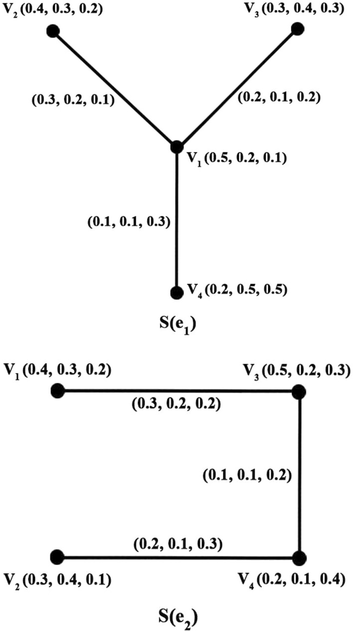
Picture fuzzy soft graph $G=\{S(e_1),S(e_2)\}$

Definition 17

A Picture fuzzy soft path P in PFSG $G=(G^{\ast },F,K,O)$ is a sequence of distinct vertices $x_o,x_1,\dots ,x_n$ $(except{x}_o$ & $x_1)$ such that $({\mu }_{k(o)}(x_{i-1},x_i),$ ${\gamma }_{k(o)}(x_{i-1},x_i),{\sigma }_{k(o)}(x_{i-1},x_i))>0$, $i=1,\dots n$ Here n denotes the length of the PFSP. The successive pairs are called the edges of PFSP. For example, in Fig. 1, consider $S(e_1)$ then $v_2,v_1$ is a PFSP.

Definition 18

The diameter of $a,b\in V,$ is the length of the longest PFSP joining a to b. The strength of P is defined as $\left({\displaystyle \underset{i=1}{\overset{n}{\bigwedge }}{\mu }_{k(o)}(x_{i-1},x_i),\underset{i=1}{\overset{n}{\bigwedge }}{\gamma }_{k(o)}(x_{i-1},x_i),\underset{i=1}{\overset{n}{\bigvee }}{\sigma }_{k(o)}(x_{i-1},x_i)}\right).$ The strength of the PFSP is the weight of the weakest edges and represented by d(P). The strength of connectedness between two vertices a & b is defined as the maximum of the strengths of all PFSP’s between a and b and represented by ${\mathrm{PFSCONN}}_G(a,b).$

Definition 19

The PFSG $G_1=(G^{\ast },F_1,K_1,T)$ is called a spanning PFSSG of $G=(G^{\ast },F,K,O)$ if

$(\mathrm{i})T\subseteq O$

$(\mathrm{ii})$$\begin{array}{cc}\hfill {\mu }_{F_1(z)}(q)=& {\mu }_{F_{(}z)}(q),\hfill \\ \hfill {\gamma }_{F_1(z)}(q)=& {\gamma }_{F_{(}z)}(q),\hfill \\ \hfill {\sigma }_{F_1(z)}(q)=& {\sigma }_{F_{(}z)}(q)\forall z\in O,q\in V.\hfill \end{array}$

Definition 20

The order of a picture fuzzy soft graph is

$$\begin{array}{cc}& {\displaystyle O(G)=(\sum _{e_i\in O}\left({\displaystyle \sum _{u\in V}{\mu }_{F(e_i)}(u)}\right),\sum _{e_i\in O}\left({\displaystyle \sum _{u\in V}{\gamma }_{F(e_i)}(u)}\right),}\hfill \\ \hfill & {\displaystyle \sum _{e_i\in O}\left({\displaystyle \sum _{u\in V}{\sigma }_{F(e_i)}(u)}\right).}\hfill \end{array}$$

The size of picture fuzzy soft graph is

$$\begin{array}{c}\hfill {\displaystyle S(G)=(\sum _{e_i\in O}\left({\displaystyle \sum _{uv\in E}{\mu }_{K(e_i)}(uv)}\right),\sum _{e_i\in O}\left({\displaystyle \sum _{uv\in E}{\gamma }_{K(e_i)}(uv)}\right),}\\ \hfill {\displaystyle \sum _{e_i\in O}\left({\displaystyle \sum _{uv\in E}{\sigma }_{K(e_i)}(uv)}\right).}\end{array}$$

Example 21

Consider a crisp graph $G^{\ast }=(V,E)$ such that $V=\{v_1,v_2,v_3,v_4,v_5\}$ and $E=\{v_1{v}_2,v_2{v}_3,v_2{v}_4,$ $v_4{v}_5,v_1{v}_5,v_3{v}_5\}.$ Let $O=\{e_1,e_2,e_3\}$ be a parameter set and let (F, O) be Picture fuzzy soft set over V with $F:O\to P(V)$ defined by

$$\begin{array}{cc}& F(e_1)=\{(v_1,0.4,0.3,0.3),(v_2,0.2,0.2,0.3),(v_3,0.2,0.1,0.1),\hfill \\ \hfill & (v_4,0.1,0.3,0.2),(v_5,0.3,0.4,0.1)\}\hfill \\ \hfill & F(e_2)=\{(v_1,0.4,0.3,0.2),(v_2,0.3,0.2,0.3),(v_3,0.4,0.1,0.2),\hfill \\ \hfill & (v_4,0.1,0.1,0.2),(v_5,0.2,0.4,0.1)\}\hfill \\ \hfill & F(e_3)=\{(v_1,0.3,0.4,0.2),(v_2,0.3,0.2,0.1),(v_3,0.3,0.4,0.1),\hfill \\ \hfill & (v_4,0.4,0.2,0.1),(v_5,0.3,0.2,0.4)\}.\hfill \end{array}$$

Let (K, O) be picture fuzzy soft set over E with $K:O\to P(E)$ defined by

$$\begin{array}{cc}& K(e_1)=\{(v_1{v}_2,0.1,0.2,0.3),(v_2{v}_3,0.2,0.1,0.2),(v_2{v}_4,0.1,0.2,0.2),\hfill \\ \hfill & (v_4{v}_5,0.1,0.3,0.2),(v_1{v}_5,0.3,0.3,0.2),(v_3{v}_5,0.2,0.1,0.1)\}\hfill \\ \hfill & K(e_2)=\{(v_1{v}_2,0.3,0.2,0.2),(v_2{v}_3,0.3,0.1,0.3),(v_2{v}_4,0.1,0.2,0.3),\hfill \\ \hfill & (v_4{v}_5,0.1,0.1,0.2),(v_1{v}_5,0.2,0.3,0.2),(v_3{v}_5,0.2,0.1,0.2)\}\hfill \\ \hfill & K(e_3)=\{(v_1{v}_2,0.3,0.2,0.2),(v_2{v}_3,0.3,0.2,0.1),(v_2{v}_4,0.2,0.2,0.1),\hfill \\ \hfill & (v_4{v}_5,0.3,0.2,0.3),(v_1{v}_5,0.2,0.2,0.3),(v_3{v}_5,0.3,0.2,0.3)\}0.\hfill \end{array}$$

The Picture fuzzy graphs of G are $S(e_1)=(F(e_1),K(e_1)),$ $S(e_2)=(F(e_2),K(e_2)),$ and $S(e_3)$ $=(F(e_3),K(e_3))$ according to the parameters $e_1,e_2$ and $e_3$, respectively. Thus, $G=S(e_1),S(e_2),S(e_3)$ is a picture fuzzy soft graph on O.

The order of Picture fuzzy soft graph is $O(G)=((0.4+0.2+0.2+0.1+0.3)+(0.4+0.3+0.4+0.1+0.2)+(0.3+0.3+0.3+0.4+0.3),(0.3+0.2+0.1+0.3+0.4)+(0.3+0.2+0.1+0.1+0.4)+(0.4+0.2+0.4+0.2+0.2),(0.3+0.3+0.1+0.2+0.1)+(0.2+0.3+0.2+0.2+0.1)+(0.2+0.1+0.1+0.1+0.4))=(4.2,3.8,2.9)$

The size of the Picture fuzzy soft graph S(G) is $((0.1+0.2+0.1+0.1+0.3+0.2)+(0.3+0.3+0.1+0.1+0.2+0.2)+(0.3+0.3+0.2+0.3+0.2+0.3),(0.2+0.1+0.2+0.3+0.3+0.1)+(0.2+0.1+0.1+0.1+0.3+0.1)+(0.2+0.2+0.2+0.2+0.2+0.2),(0.3+0.2+0.2+0.2+0.2+0.1)+(0.2+0.3+0.3+0.2+0.2+0.2)+(0.2+0.1+0.1+0.3+0.3+0.3))$ $=(3.8,3.3,3.9)$

Regularity of picture fuzzy soft graphs

Definition 22

Let G be a Picture fuzzy soft graph of $G^{\ast }.$ G is called a regular picture fuzzy soft graph if S(e) is a regular picture fuzzy graph. $\forall$ $e\in O.$

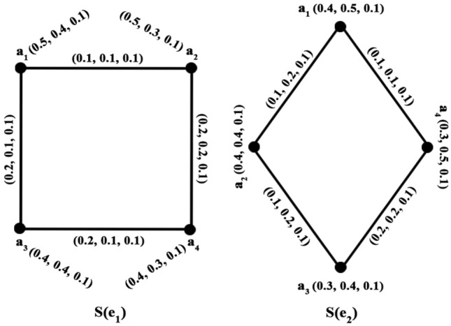
Example 23

Consider a simple graph $G^{\ast }=(V,E)$ where $V=\left\{v_1,,,v_2,,,v_3,,,v_4\right\}$ and $E=\{v_1{v}_2,v_2{v}_3,v_3{v}_4,v_4{v}_1\}.$ Let $O=\left\{e_1,,,e_2\right\}$ be a set of parameters. Let (S, O) be a picture fuzzy soft graph, where picture fuzzy graphs $S(e_1),S(e_2)$ corresponding to parameters $e_1,e_2,e_3$ & $e_4$, receptively, are

$$\begin{array}{cc}& S(e_1)=(\{(v_1,.5,.4,.1),(v_2,.4,.3,.2),\hfill \\ \hfill & (v_3,.4,.3,.2),(v_4,.3,.4,.1)\},\hfill \\ \hfill & \{(v_1{v}_2,.3,.3,.1),(v_2{v}_3,.3,.2,.1),\hfill \\ \hfill & (v_3{v}_4,.3,.3,.1),(v_4{v}_1,.3,.2,.1)\})\hfill \\ \hfill & S(e_2)=(\{(v_1,.5,.4,.2),(v_2,.4,.3,.3),\hfill \\ \hfill & (v_3,.4,.3,.2),(v_4,.3,.4,.1)\},\hfill \\ \hfill & \{(v_1{v}_2,.3,.2,.2),(v_2{v}_3,.2,.3,.1),\hfill \\ \hfill & (v_3{v}_4,.3,.2,.2),(v_4{v}_1,.2,.3,.1)\})\hfill \end{array}$$

The regular picture fuzzy graph is drawn in Fig. 2.

Fig. 2.

Regular Picture fuzzy soft graph $G=\{S(e_1),S(e_2)\}$

Definition 24

Let G be a picture fuzzy soft graph of $G^{\ast }$. G is said to be totally regular picture fuzzy soft graph if S(e) is a totally picture fuzzy graph for all $e\in O.$

Example 25

Consider a simple graph $G^{\ast }=(V,E),$ where $V=\{a_1,a_2,a_3,a_4\}$ and $E=\{a_1{a}_2,a_2{a}_3,$ $a_3{a}_4,a_1{a}_3\}$. Let $O=\left\{e_1,,,e_2\right\}$ be a set of parameters. Let $G=(S,O)$ be a picture fuzzy soft graphs, where $S(e_1)=(F(e_1),K(e_1))$ and $S(e_2)=(F(e_2),K(e_2))$ corresponding to the parameters $e_1$ and $e_2,$ respectively are defined as

$$\begin{array}{cc}& S(e_1)=(\{(a_1,.5,.4,.1),(a_2,.5,.3,.1),\hfill \\ \hfill & (a_3,.4,.4,.1),a_4,.4,.3,.1)\},\hfill \\ \hfill & \{(a_1{a}_2,.1,.1,.1),(a_2{a}_4,.2,.2,.1),\hfill \\ \hfill & (a_3{a}_4,.2,.1,.1),(a_3{a}_1,.2,.1,.1)\})\hfill \\ \hfill & S(e_2)=(\{(a_1,.4,.5,.1),(a_2,.3,.5,.1),\hfill \\ \hfill & (a_3,.4,.4,.1),a_4,.3,.4,.1)\},\hfill \\ \hfill & \{(a_1{a}_2,.1,.1,.1),(a_2{a}_4,.2,.2,.1),\hfill \\ \hfill & (a_3{a}_4,.1,.2,.1),(a_3{a}_1,.1,.2,.1)\})\hfill \end{array}$$

The totally regular picture fuzzy soft graph is drawn in Fig. 3.

Fig. 3.

Totally regular picture fuzzy soft graph $G=\{S(e_1),S(e_2)\}$

Definition 26

Let G be a Picture fuzzy soft graph on V. Then G is called as perfectly regular picture fuzzy soft graph if $S(e_i)$ is a regular and totally regular picture fuzzy graph for all $e_i\in O.$

Proposition 27

For a perfectly regular picture fuzzy soft graph $G=(F,K,O)$, F is a constant function.

Theorem 28

Let G be a picture fuzzy soft graph. Then G is perfectly regular if and only if

1. ${\displaystyle \sum _{a\ne b}{\mu }_{K(e_i)}(ab)=\sum _{c\ne b}{\mu }_{K(e_i)}(bc),}$

${\displaystyle \sum _{a\ne b}{\gamma }_{K(e_i)}(ab)=\sum _{c\ne b}{\gamma }_{K(e_i)}(bc),}$

${\displaystyle \sum _{a\ne b}{\sigma }_{K(e_i)}(ab)=\sum _{c\ne b}{\sigma }_{K(e_i)}(bc).}$

2. ${\mu }_{F(e_i)}(a)={\mu }_{K(e_i)}(b),$

${\gamma }_{F(e_i)}(a)={\gamma }_{K(e_i)}(b),$

${\sigma }_{F(e_i)}(a)={\sigma }_{K(e_i)}(b)$ $\forall$ $a,b\in V,$ $e_i\in O.$

Proof

Assume G is perfectly regular picture fuzzy soft graph. So G is regular picture fuzzy soft graph. Thus, from definition we have ${\mathrm{deg}}_{\mu }(a)={\mathrm{deg}}_{\mu }(c),$ ${\mathrm{deg}}_{\gamma }(a)=de{g}_{\gamma }(c),$ ${\mathrm{deg}}_{\sigma }(a)={\mathrm{deg}}_{\sigma }(c),$ $\forall$ $a,c\in V$ $e_i\in O.$ Then

$$\begin{array}{cc}\hfill {\displaystyle \sum _{a\ne b}{\mu }_{K(e_i)}(ab)=}& {\displaystyle \sum _{c\ne b}{\mu }_{K(e_i)}(bc),}\hfill \\ \hfill {\displaystyle \sum _{a\ne b}{\gamma }_{K(e_i)}(ab)=}& {\displaystyle \sum _{c\ne b}{\gamma }_{K(e_i)}(cb),}\hfill \\ \hfill {\displaystyle \sum _{a\ne b}{\sigma }_{K(e_i)}(ab)=}& {\displaystyle \sum _{c\ne b}{\sigma }_{K(e_i)}(bc)\forall a,b,C\in V,e_i\in O.}\hfill \end{array}$$

Thus (1) holds. By the proposition (3.14), (2) also holds.

Conversely, suppose that G is a picture fuzzy soft graph such that it satisfies the conditions. From (1), we have

$$\begin{array}{cc}\hfill {\displaystyle \sum _{a\ne b}{\mu }_{K(e_i)}(ab)=}& {\displaystyle \sum _{c\ne b}{\mu }_{K(e_i)}(bc),}\hfill \\ \hfill {\displaystyle \sum _{a\ne b}{\gamma }_{K(e_i)}(ab)=}& {\displaystyle \sum _{c\ne b}{\gamma }_{K(e_i)}(bc),}\hfill \\ \hfill {\displaystyle \sum _{a\ne b}{\sigma }_{K(e_i)}(ab)=}& {\displaystyle \sum _{c\ne b}{\sigma }_{K(e_i)}(bc)\forall a,b,c\in V,e_i\in O.}\hfill \end{array}$$

${\mathrm{deg}}_{\mu }(a)={\mathrm{deg}}_{\mu }(c)=r_i,$ ${\mathrm{deg}}_{\gamma }(a)={\mathrm{deg}}_{\gamma }(c)=r_i^{\prime },$ and ${\mathrm{deg}}_{\sigma }(a)={\mathrm{deg}}_{\sigma }(c)=r_i^{\prime \prime },$ $\forall$ $c,a\in V,$ $e_i\in O.$ This implies $S(e_i)$ is a regular picture fuzzy graph. Thus, G is a regular picture fuzzy soft graph.

From (2), ${\mu }_{F(e_i)}(a)={\mu }_{F(e_i)}(c)=x_i,$ ${\gamma }_{F(e_i)}(a)={\gamma }_{F(e_i)}$ $(c)=x_i^{\prime },$ and ${\sigma }_{F(e_i)}(a)={\sigma }_{F(e_i)}(c)=x_i^{\prime \prime },$ $\forall$ $c,a\in V,$ $e_i\in O.$

Thus, F is a constant function

$$\begin{array}{cc}& {\mathrm{deg}}_{\mu }[c]={\mathrm{deg}}_{\mu }(c)+{\mu }_{F(e_i)}(c)=r_i+x_i,\hfill \\ \hfill & {\mathrm{deg}}_{\mu }[d]={\mathrm{deg}}_{\mu }(d)+{\mu }_{F(e_i)}(d)=r_i+x_i.\hfill \\ \hfill & {\mathrm{deg}}_{\gamma }[c]={\mathrm{deg}}_{\gamma }(c)+{\gamma }_{F(e_i)}(c)=r_i^{\prime }+x_i^{\prime },\hfill \\ \hfill & {\mathrm{deg}}_{\gamma }[d]={\mathrm{deg}}_{\gamma }(c)+{\gamma }_{F(e_i)}(d)=r_i^{\prime }+x_i^{\prime }.\hfill \\ \hfill & {\mathrm{deg}}_{\sigma }[c]={\mathrm{deg}}_{\sigma }(c)+{\sigma }_{F(e_i)}(c)=r_i^{\prime \prime }+x_i^{\prime \prime },\hfill \\ \hfill & {\mathrm{deg}}_{\sigma }[d]={\mathrm{deg}}_{\sigma }(c)+{\sigma }_{F(e_i)}(d)=r_i^{\prime \prime }+x_i^{\prime \prime }.\hfill \\ \hfill & \forall c,d\in V,e_i\in O.\hfill \end{array}$$

${\mathrm{deg}}_{\mu }[c]={\mathrm{deg}}_{\mu }[d]=k_i,$ ${\mathrm{deg}}_{\gamma }[c]={\mathrm{deg}}_{\gamma }[d]=k_i^{\prime }$ and ${\mathrm{deg}}_{\sigma }[c]={\mathrm{deg}}_{\sigma }[d]=k_i^{\prime \prime }.$ (ie) $\mathrm{deg}[c]=\mathrm{deg}[d]=(k_i,k_i^{\prime },k_i^{\prime \prime })$ $\forall$ $c,d\in V,$ $e_i\in O.$ So $S(e_i)$ is a totally regular picture fuzzy graph.

Hence, G is totally regular picture fuzzy soft graph. This implies G is a perfect picture fuzzy soft graph. $\square$

Corollary 29

If G is a perfectly regular picture fuzzy soft graph and $F=\left({\mu }_{F(e_i)},(c),,,{\gamma }_{F(e_i)},(c),,,{\sigma }_{F(e_i)},(c)\right)=\left(r_i,,,r_i^{\prime },,,r_i^{\prime \prime }\right)$, $\forall$ $c\in V,$ $e_i\in O$ is a constant function in $S(e_i)$ then $O(S(e_i))=|V|\left(r_i,,,r_i^{\prime },,,r_i^{\prime \prime }\right).$

Theorem 30

Let $G=(F,K,O)$ be a perfectly regular picture fuzzy soft graph. Then size of $S(e_i)$ is $S(S(e_i))=\frac{|V|}{2}(x_i,x_i^{\prime },x_i^{\prime \prime }),$ where $(x_i,x_i^{\prime },x_i^{\prime \prime })$ is the degree of a vertex in $S(e_i)$ $\forall$ $e_i\in O.$

Operations of picture soft graphs

Definition 31

Let $G_1=(F_1,K_1,O)$ and $G_2=(F_2,K_2,T)$ be two PFSG of $G_1^{\ast }=(V_1,E_1)$, $G_2^{\ast }=(V_2,E_2)$. The Cartesian Product of $G_1$, $G_2$ is a PFSG $G:G_1\times G_2=(F,K,O\times T)$, where $(F=F_1\times F_2,O\times T)$ is a PFSS over $V=V_1\times V_2,$ $(K=K_1\times K_2,O\times T)$ is a PFSS over $E=\{((y,z_1),(y,z_2)):y\in V_1,(z_1,z_2)\in E_2\}\cup \{((y_1,z),(y_2,z)):z\in V_2,(y_1,y_2)\in E_1\}$ and $(F,K,O\times T)$ are PFSG such that

1. $\begin{array}{cc}& {\mu }_{F(d,k)}(y,z)={\mu }_{F_1(d)}(y)\wedge {\mu }_{F_2(k)}(z)\hfill \\ \hfill & {\gamma }_{F(d,k)}(y,z)={\gamma }_{F_1(d)}(y)\wedge {\gamma }_{F_2(k)}(z)\hfill \\ \hfill & {\sigma }_{F(d,k)}(y,z)={\sigma }_{F_1(d)}(y)\vee {\sigma }_{F_2(k)}(z)\hfill \\ \hfill & \forall (y,z)\in V,(d,k)\in O\times T\hfill \end{array}$

2. $\begin{array}{cc}& {\mu }_{K(d,k)}(({y,z}_1),({y,z}_2))={\mu }_{F_1(d)}(y)\wedge {\mu }_{K_2(k)}({z_1,z}_2)\hfill \\ \hfill & {\gamma }_{K(d,k)}(({y,z}_1),({y,z}_2))={\gamma }_{F_1(d)}(y)\wedge {\gamma }_{K_2(k)}({z_1,z}_2)\hfill \\ \hfill & {\sigma }_{K(d,k)}(({y,z}_1),({y,z}_2))={\sigma }_{F_1(d)}(y)\vee {\sigma }_{K_2(k)}({z_1,z}_2)\hfill \\ \hfill & \forall y\in V_1,{({z_1,z}_2)\in E}_2\hfill \end{array}$

3. $\begin{array}{cc}& {\mu }_{K(d,k)}((y_1,z),(y_2,z))={\mu }_{F_2(k)}(z)\wedge {\mu }_{K_1(d)}({y_1,y}_2)\hfill \\ \hfill & {\gamma }_{K(d,k)}((y_1,z),(y_2,z))={\gamma }_{F_2(k)}(z)\wedge {\gamma }_{K_1(d)}({y_1,y}_2)\hfill \\ \hfill & {\sigma }_{K(d,k)}((y_1,z),(y_2,z))={\sigma }_{F_2(k)}(z)\vee {\sigma }_{K_1(d)}({y_1,y}_2)\hfill \\ \hfill & \forall z\in V_2,{({y_1,y}_2)\in E}_2\hfill \end{array}$ $S(d,k)=S_1(d)\times S_2(k)$ $\forall$ $(d,k)\in O\times T$ are picture fuzzy graphs of G.

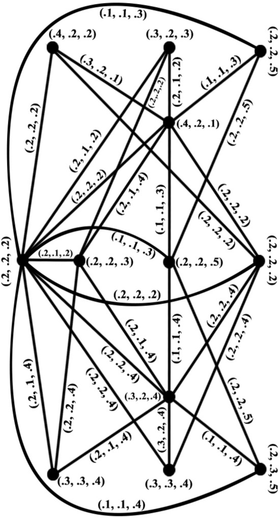
Example 32

Let $O=\{e_1,e_2\}$ and $T=\{e_3,e_4\}$ be the set of parameters. Consider two PFSG’s $G_1=\{S_1(e_1),$ $S_1(e_2)\}$ and $G_2=\{S_2(e_3),S_2(e_4)\}$ as in Figs. 4, 5, 6, 7.

Fig. 4.

Picture fuzzy soft graph $S_1(e_1)$

Fig. 5.

Picture fuzzy soft graph $S_1(e_2)$

Fig. 6.

Picture fuzzy soft graph $S_2(e_3)$

Fig. 7.

Picture fuzzy soft graph $S_2(e_4)$

The Cartesian product of $G_1$ and $G_2$ is $G_1\times G_2=S,O\times T$, where $O\times T=(e_1,e_3),(e_1,e_4),(e_2,e_3),(e_2,e_4),S(e_1,e_3)=S_1(e_1)\times S_2(e_3),S(e_1,e_4)=S_1(e_1)\times S_2(e_4),S(e_2,e_3)=S_1(e_2)\times S_2(e_3)$ and $S(e_2,e_4)=S_1(e_2)\times S_2(e_4)$ are picture fuzzy soft graphs of $G_1\times G_2$. $S(e_1,e_3)=S_1(e_1)\times S_2(e_3)$ is shown in Fig. 8. In the similar way, the Cartesian product of $S(e_1,e_4)$, $S(e_2,e_3)$, $S(e_2,e_4)$ can be drawn.

Fig. 8.

Cartesian Product $S(e_1,e_3)$

Theorem 33

The Cartesian product of two PFSG is a PFSG.

Proof

Let $G_1=(F_1,K_1,O)$, $G_2=(F_2,K_2,T)$ be two PFSG of $G_1^{\ast }=(V_1,E_1)$, $G_2^{\ast }=(V_2,E_2)$, respectively. Let $G=G_1\times G_2=(F,K,O\times T)$ be the Cartesian product of $G_1$ and $G_2$. We claim that $G=(F,K,O\times T)$ is a PFSG and $(S,O\times T)=\{F_1\times F_2(a_i,b_j),K_1\times K_2(a_i,b_j)\}\forall a_i\in O,b_j\in T$ for $i=1$ to m,  $j=1$ to n are PFSG of G.

Consider

$$\begin{array}{cc}& {\mu }_{K_{(a_i,b_j)}}((h,o_1),(h,o_2))\hfill \\ \hfill & =min\{{\mu }_{F_1(a_i)}(h),{\mu }_{K_2(b_j)}(o_1,o_2)\}\hfill \\ \hfill & \text{for}i=1\text{to}m,j=1\text{to}n\hfill \\ \hfill & \le min\{{\mu }_{F_1(a_i)}(h),min\{{\mu }_{F_2(b_j)}(o_1),{\mu }_{F_2(b_j)}(o_2)\}\}\hfill \\ \hfill & =min\{min\{{\mu }_{F_1(a_i)}(h),{\mu }_{F_2(b_j)}(o_1)\},\hfill \\ \hfill & min\{{\mu }_{F_1(a_i)}(h),{\mu }_{F_2(b_j)}(o_2)\}\}\hfill \\ \hfill & {\mu }_{K_{(a_i,b_j)}}((h,o_1),(h,o_2))\le min\{({\mu }_{F_1(a_i)}\times {\mu }_{F_2(b_j)})(h,o_1),\hfill \\ \hfill & ({\mu }_{F_1(a_i)}\times {\mu }_{F_2(b_j)})(h,o_2)\},\hfill \end{array}$$

$i=1$ to m, $j=1$ to n.

$$\begin{array}{cc}& {\gamma }_{K_{(a_i,b_j)}}((h,o_1),(h,o_2))\hfill \\ \hfill & =min\{{\gamma }_{F_1(a_i)}(h),min\{{\gamma }_{F_2(b_j)}(o_1),{\gamma }_{F_2(b_j)}(o_2)\}\}\hfill \\ \hfill & =min\{min\{{\gamma }_{F_1(a_i)}(h),{\gamma }_{F_2(b_j)}(o_1)\}\hfill \\ \hfill & min\{{\gamma }_{F_1(a_i)}(h),{\gamma }_{F_2(b_j)}(o_2)\}\}\hfill \\ \hfill & {\sigma }_{K_{(a_i,b_j)}}((h,o_1),(h,o_2))\hfill \\ \hfill & =max\{{\sigma }_{F_1(a_i)}(h),{\sigma }_{F_2(b_j)}(o_1,o_2)\}\hfill \\ \hfill & \text{for}i=1\text{to}m,j=1\text{to}n\hfill \\ \hfill & \le max\{{\sigma }_{F_1(a_i)}(h),max\{{\sigma }_{F_2(b_j)}(o_1),{\sigma }_{F_2(b_j)}(o_2)\}\}\hfill \\ \hfill & =max\{max\{{\sigma }_{F_1(a_i)}(h),{\sigma }_{F_2(b_j)}(o_1)\},\hfill \\ \hfill & max\{{\sigma }_{F_1(a_i)}(h),{\sigma }_{F_2(b_j)}(o_2)\}\}\hfill \\ \hfill & {\sigma }_{K_{(a_i,b_j)}}((h,o_1),(h,o_2))\le max\{({\sigma }_{F_1(a_i)}\times {\sigma }_{F_2(b_j)})(h,o_1),\hfill \\ \hfill & ({\sigma }_{F_1(a_i)}\times {\sigma }_{F_2(b_j)})(h,o_2)\},\hfill \end{array}$$

$i=1$ to m, $j=1$ to n.

Similarly,

$$\begin{array}{cc}& {\mu }_{K_{(a_i,b_j)}}((h_1,o),(h_2,o))\le min\{({\mu }_{F_1(a_i)}\times {\mu }_{F_2(b_j)})(h_1,o),\hfill \\ \hfill & ({\mu }_{F_1(a_i)}\times {\mu }_{F_2(b_j)})(h_2,o)\},\hfill \end{array}$$

$i=1$ to m, $j=1$ to n.

$$\begin{array}{cc}& {\gamma }_{K_{(a_i,b_j)}}((h_1,o),(h_2,o))\le min\{({\gamma }_{F_1(a_i)}\times {\gamma }_{F_2(b_j)})(h_1,o),\hfill \\ \hfill & ({\gamma }_{F_1(a_i)}\times {\gamma }_{F_2(b_j)})(h_2,o)\},\hfill \end{array}$$

$i=1$ to m, $j=1$ to n.

$$\begin{array}{cc}& {\sigma }_{K_{(a_i,b_j)}}((h_1,o),(h_2,o))\le max\{({\sigma }_{F_1(a_i)}\times {\sigma }_{F_2(b_j)})(h_1,o),\hfill \\ \hfill & ({\sigma }_{F_1(a_i)}\times {\sigma }_{F_2(b_j)})(h_2,o)\},\hfill \end{array}$$

$i=1$ to m, $j=1$ to n.

Therefore $G=(F,K,O\times T)$ is PFSG. $\square$

Definition 34

The cross product of $G_1$ & $G_2$ is $G=G_1\circ G_2=(F,K,O\times T)$, where $(F,O\times T)$ is a PFSS over $V=V_1\times V_2,$ $(K,O\times T)$ is a PFSS over $E=\{((y_1,z_1),((y_2,z_2)):(y_1,y_2)\in E_1,(z_1,z_2)\in E_2\}$ and $(F,K,O\times T)$ are PFSG such that

1. $$\begin{array}{cc}& {\mu }_{F(d,h)}(y,z)={\mu }_{F_1(d)}(y)\wedge {\mu }_{F_2(h)}(z)\hfill \\ \hfill & {\gamma }_{F(d,h)}(y,z)={\gamma }_{F_1(d)}(y)\wedge {\gamma }_{F_2(h)}(z)\hfill \\ \hfill & {\sigma }_{F(d,h)}(y,z)={\sigma }_{F_1(d)}(y)\vee {\sigma }_{F_2(h)}(z)\hfill \\ \hfill & \forall (y,z)\in V,(d,h)\in O\times T.\hfill \end{array}$$
2. $$\begin{array}{cc}& {\mu }_{K(d,h)}((y_1,z_1),(y_2,z_2))\hfill \\ \hfill & ={\mu }_{K_1(d)}(y_1,y_2)\wedge {\mu }_{K_2(h)}({z_1,z}_2)\hfill \\ \hfill & {\gamma }_{K(d,h)}((y_1,z_1),(y_2,z_2))\hfill \\ \hfill & ={\gamma }_{K_1(d)}(y_1,y_2)\wedge {\gamma }_{K_2(h)}({z_1,z}_2)\hfill \\ \hfill & {\sigma }_{K(d,h)}((y_1,z_1),(y_2,z_2))\hfill \\ \hfill & ={\sigma }_{K_1(d)}(y_1,y_2)\vee {\sigma }_{K_2(h)}({z_1,z}_2)\hfill \\ \hfill & \forall (y_1,y_2)\in V_1,{({z_1,z}_2)\in E}_2\hfill \end{array}$$

$S(d,h)=S_1(d)\circ S_2(h)$ $\forall$ $(d,h)\in O\times T$ are PFSG of G.

Example 35

Let $O=\{e_1,e_2\}$ and $T=\{e_3,e_4\}$ be the set of parameters. Consider two PFSG’s $G_1=\{S_1(e_1),$ $S_1(e_2)\}$ and $G_2=\{S_2(e_3),S_2(e_4)\}$ as in Figs. 4, 5, 6, 7.

The Cross product of $G_1$ and $G_2$ is $G_1\times G_2=S,O\times T$, where $O\times T=(e_1,e_3),(e_1,e_4),(e_2,e_3),(e_2,e_4),S(e_1,e_3)=S_1(e_1)\times S_2(e_3),S(e_1,e_4)=S_1(e_1)\times S_2(e_4),S(e_2,e_3)=S_1(e_2)\times S_2(e_3)$ and $S(e_2,e_4)=S_1(e_2)\times S_2(e_4)$ are picture fuzzy soft graphs of $G_1\times G_2$. $S(e_1,e_3)=S_1(e_1)\times S_2(e_3)$ is shown in Fig. 9. In the similar way the cross product of $S(e_1,e_4)$, $S(e_2,e_3)$, $S(e_2,e_4)$ can be drawn.

Fig. 9.

Cross product $S(e_1,e_3)$

Theorem 36

The cross product of two PFSG is also a PFSG.

Proof

Let $G_1=(F_1,K_1,O)$ & $G_2=(F_2,K_2,T)$ be PFSG of $G_1^{\ast }=(V_1,E_1)$ & $G_2^{\ast }=(V_2,E_2)$, respectively. Let the cross product be $G=G_1\circ G_2=(F,K,O\times T).$ We claim that $G=(F,K,O\times T)$ is a PFSG and $(S,O\times T)=\{F_1\circ F_2(a_i,b_j),K_1\circ K_2(a_i,b_j)\}$ $\forall$ $a_i$ in O, $b_j$ in T for $i=1$ to m,  $j=1$ to n are PFSG of G.

Consider

$$\begin{array}{cc}& {\mu }_{K_{(a_i,b_j)}}((c_1,t_1),(c_2,t_2))\hfill \\ \hfill & =min\{{\mu }_{K_1(a_i)}(c_1,c_2),{\mu }_{K_2(b_j)}(t_1,t_2)\}\hfill \end{array}$$

for $i=1$ to m,  $j=1$ to n

$$\begin{array}{cc}& \le min\{min\{{\mu }_{F_1(a_i)}(c_1),{\mu }_{F_1(a_i)}(c_2)\},\hfill \\ \hfill & min\{{\mu }_{F_2(b_j)}(t_1),{\mu }_{F_2(b_j)}(t_2)\}\}\hfill \\ \hfill & =min\{min\{{\mu }_{F_1(a_i)}(c_1),{\mu }_{F_2(b_j)}(t_1)\},\hfill \\ \hfill & min\{{\mu }_{F_1(a_i)}(c_2),{\mu }_{F_2(b_j)}(t_2)\}\}\hfill \\ \hfill & {\mu }_{K_{(a_i,b_j)}}((c_1,t_1),(c_2,t_2))\le min\{({\mu }_{F_1(a_i)}\circ {\mu }_{F_2(b_j)})(c_1,t_1),\hfill \\ \hfill & ({\mu }_{F_1(a_i)}\circ {\mu }_{F_2(b_j)})(c_2,t_2)\}\hfill \end{array}$$

for $i=1$ to m, $j=1$ to n.

$$\begin{array}{cc}& {\gamma }_{K_{(a_i,b_j)}}((c_1,t_1),(c_2,t_2))\hfill \\ \hfill & =min\{{\gamma }_{K_1(a_i)}(c_1,c_2),{\gamma }_{K_2(b_j)}(t_1,t_2)\}\hfill \end{array}$$

for $i=1$ to m, $j=1$ to n.

$$\begin{array}{cc}& \le min\{min\{{\gamma }_{F_1(a_i)}(c_1),{\gamma }_{F_1(a_i)}(c_2)\},\hfill \\ \hfill & min\{{\gamma }_{F_2(b_j)}(t_1),{\gamma }_{F_2(b_j)}(t_2)\}\}\hfill \\ \hfill & =min\{min\{{\gamma }_{F_1(a_i)}(c_1),{\gamma }_{F_2(b_j)}(t_1)\}\},\hfill \\ \hfill & \{min\{{\gamma }_{F_1(a_i)}(c_2),{\gamma }_{F_2(b_j)}(t_2)\}\}\hfill \\ \hfill & {\sigma }_{K_{(a_i,b_j)}}((c_1,t_1),(c_2,t_2))\le min\{({\gamma }_{F_1(a_i)}\circ {\gamma }_{F_2(b_j)})(c_1,t_1),\hfill \\ \hfill & {\gamma }_{F_2(a_i)}\circ {\gamma }_{F_2(b_j)}(c_2,t_2)\}\hfill \\ \hfill \end{array}$$

for $i=1$ to m, $j=1$ to n.

$$\begin{array}{cc}& {\sigma }_{K_{(a_i,b_j)}}((c_1,t_1),(c_2,t_2))\hfill \\ \hfill & =max\{{\sigma }_{K_1(a_i)}(c_1,c_2),{\sigma }_{K_2(b_j)}(t_1,t_2)\}\hfill \end{array}$$

for $i=1$ to m, $j=1$ to n.

$$\begin{array}{cc}& \le max\{max\{{\sigma }_{F_1(a_i)}(c_1),{\sigma }_{F_1(a_i)}(c_2)\},\hfill \\ \hfill & max\{{\sigma }_{F_2(b_j)}(t_1),{\sigma }_{F_2(b_j)}(t_2)\}\}\hfill \\ \hfill & =max\{max\{{\sigma }_{F_1(a_i)}(c_1),{\sigma }_{F_2(b_j)}(t_1)\},\hfill \\ \hfill & max\{{\sigma }_{F_1(a_i)}(c_2),{\sigma }_{F_2(b_j)}(t_2)\}\}\hfill \\ \hfill & {\sigma }_{K_{(a_i,b_j)}}((c_1,t_1),(c_2,t_2))\le max\{({\sigma }_{F_1(a_i)}\circ {\sigma }_{F_2(b_j)})(c_1,t_1),\hfill \\ \hfill & {\sigma }_{F_2(a_i)}\circ {\sigma }_{F_2(b_j)}(c_2,t_2)\}\hfill \end{array}$$

for $i=1$ to m, $j=1$ to n.

Hence, $G=(F,K,O\times T)$ is a PFSG. $\square$

Definition 37

The lexicographic product of $G_1$ & $G_2$ is $G=G_1⨀G_2=(F,K,O\times T),$ where $(F,O\times T)$ is PFSS over $V=V_1\times V_2,(K,O\times T)$ is a PFSS over $E=\{((c,h_1),((c,h_2)):c\in V_1,(h_1,h_2)\in E_2\}\cup \{((c_1,h_1),((c_2,h_2)):(c_1,h_1)\in E_1,(c_2,h_2)\in E_2\}$ and $(F,K,O\times T)$ are PFSG such that

1. $$\begin{array}{cc}& {\mu }_{F(p,q)}(c,h)={\mu }_{F_1(p)}(c)\wedge {\mu }_{F_2(q)}(h)\hfill \\ \hfill & {\gamma }_{F(p,q)}(c,h)={\gamma }_{F_1(p)}(c)\wedge {\gamma }_{F_2(q)}(h)\hfill \\ \hfill & {\sigma }_{F(p,q)}(c,h)={\sigma }_{F_1(p)}(c)\vee {\sigma }_{F_2(q)}(h)\hfill \\ \hfill & \forall (c,h)\in V,(p,q)\in O\times T.\hfill \end{array}$$
2. $$\begin{array}{cc}& {\mu }_{K(p,q)}((c,h_1),(c,h_2))={\mu }_{F_1(p)}(c)\wedge {\mu }_{K_2(q)}({h_1,h}_2)\hfill \\ \hfill & {\gamma }_{K(p,q)}((c,h_1),(c,h_2))={\gamma }_{F_1(p)}(c)\wedge {\gamma }_{K_2(q)}({h_1,h}_2)\hfill \\ \hfill & {\sigma }_{K(p,q)}((c,h_1),(c,h_2))={\sigma }_{F_1(p)}(c)\vee {\sigma }_{K_2(q)}({h_1,h}_2)\hfill \\ \hfill & \forall c\in V_1,{({h_1,h}_2)\in E}_2.\hfill \end{array}$$
3. $$\begin{array}{cc}& {\mu }_{K(p,q)}((c_1,h_1),(c_2,h_2))\hfill \\ \hfill & ={\mu }_{K_1(p)}(c_1,c_2)\wedge {\mu }_{K_2(q)}({h_1,h}_2)\hfill \\ \hfill & {\gamma }_{K(p,q)}((c_1,h_1),(c_2,h_2))\hfill \\ \hfill & ={\gamma }_{K_1(p)}(c_1,c_2)\wedge {\gamma }_{K_2(q)}({h_1,h}_2)\hfill \\ \hfill & {\sigma }_{K(p,q)}((c_1,h_1),(c_2,h_2))\hfill \\ \hfill & ={\sigma }_{K_1(p)}(c_1,c_2)\vee {\sigma }_{K_2(q)}({h_1,h}_2)\hfill \\ \hfill & \forall {({c_1,c}_2)\in E}_1,{({h_1,h}_2)\in E}_2.\hfill \end{array}$$

Example 38

Consider the graphs $G_1$ and $G_2$ from example 1. The lexico product of $S(e_1,e_3)$ is given in Fig. 10. In the similar way, the lexico product of $S(e_1,e_4)$, $S(e_2,e_3)$, $S(e_2,e_4)$ can be drawn.

Fig. 10.

Lexico product $S(e_1,e_3)$

Theorem 39

The lexicographic product of two PFSG is a PFSG.

Proof

$G_1=(F_1,K_1,O)$ and $G_2=(F_2,K_2,T)$ be PFSG of $G_1^{\ast }=(V_1,E_1)$ and $G_2^{\ast }=(V_2,E_2),$ respectively. Let $G_1⨀G_2=(F,K,O\times T),$ be composition of $G_1$ and $G_2.$ We claim that $G_1⨀G_2=G=(F,K,O\times T)$ is a PFSG and $(S,O\times T)=\{F_1(a_i)⨀F_2(b_j),K_1(a_i)⨀K_2(a_i)\}$ $\forall$ $a_i\in O,b_j\in T$ for $i=1$ to m,  $j=1$ to n are PFG of G. Let $q\in V_1$ and $(w_1,w_2)\in E_2,$ we have

$$\begin{array}{cc}& {\mu }_{K_{(a_i,b_j)}}((q,w_1),(q,w_2))\hfill \\ \hfill & =min\{{\mu }_{F_1(a_i)}(q),{\mu }_{F_2(b_j)}(w_1,w_2)\}\hfill \end{array}$$

for $i=1$ to m,  $j=1$ to n.

$$\begin{array}{cc}& {\mu }_{K_{(a_i,b_j)}}((q,w_1),(q,w_2))\hfill \\ \hfill & \le min\{{\mu }_{F_1(a_i)}(q),min\{{\mu }_{F_2(b_j)}(w_1,{\mu }_{F_2(b_j)}(w_2)\}\}\hfill \\ \hfill & =min\{min\{{\mu }_{F_1(a_i)}(q),{\mu }_{F_2(b_j)}(w_1)\},\hfill \\ \hfill & min\{{\mu }_{F_1(a_i)}(q),{\mu }_{F_2(b_j)}(w_2)\}\}\hfill \\ \hfill & =min\{({\mu }_{F_1(a_i)}\times {\mu }_{F_2(b_j)})(q,w_1),\hfill \\ \hfill & ({\mu }_{F_1(a_i)}\times {\mu }_{F_2(b_j)})(q,w_2)\}\hfill \\ \hfill & {\mu }_{K_{(a_i,b_j)}}((q,w_1),(q,w_2))\hfill \\ \hfill & \le min\{{\mu }_{F(a_i,b_j)}(q,w_1),{\mu }_{F(a_i,b_j)}(q,w_2)\}\hfill \\ \hfill & {\gamma }_{K_{(a_i,b_j)}}((q,w_1),(q,w_2))\hfill \\ \hfill & =min\{{\gamma }_{F_1(a_i)}(q),{\gamma }_{K_2(b_j)}(w_1,w_2)\}\hfill \end{array}$$

for $i=1$ to m,  $j=1$ to n.

$$\begin{array}{cc}& {\gamma }_{K_{(a_i,b_j)}}((q,w_1),(q,w_2))\le min\{min\{{\gamma }_{F_1(a_i)}(q),\hfill \\ \hfill & min\{{\gamma }_{F_2(b_j)}(w_1),{\gamma }_{F_2(b_j)}(w_2)\}\}\}\hfill \\ \hfill & =min\{min\{{\gamma }_{F_1(a_i)}(q),{\gamma }_{F_2(b_j)}(w_1)\},\hfill \\ \hfill & min\{{\gamma }_{F_1(a_i)}(q),{\gamma }_{F_2(b_j)}(w_2)\}\}\hfill \\ \hfill & =min\{({\gamma }_{F_1(a_i)}\times {\gamma }_{F_2(b_j)})(q,w_1),({\gamma }_{F_1(a_i)}\times {\gamma }_{F_2(b_j)})(q,w_2)\}\hfill \\ \hfill & {\mu }_{K_{(a_i,b_j)}}((q,w_1),(q,w_2))\hfill \\ \hfill & \le min\{{\mu }_{F(a_i,b_j)}(q,w_1),{\mu }_{F(a_i,b_j)}(q,w_2)\}\hfill \\ \hfill & {\sigma }_{K_{(a_i,b_j)}}((q,w_1),(q,w_2))\hfill \\ \hfill & =max\{{\sigma }_{F_1(a_i)}(q),{\sigma }_{K_2(b_j)}(w_1,w_2)\}\hfill \end{array}$$

for $i=1$ to m,  $j=1$ to n.

$$\begin{array}{cc}& {\sigma }_{K_{(a_i,b_j)}}((q,w_1),(q,w_2))\le max\{{\sigma }_{F_1(a_i)}(q),\hfill \\ \hfill & max\{{\sigma }_{F_2(b_j)}(w_1),{\sigma }_{F_2(b_j)}(w_2)\}\}\hfill \\ \hfill & =min\{max\{{\sigma }_{F_1(a_i)}(q),{\sigma }_{F_2(b_j)}(w_1)\},\hfill \\ \hfill & max\{{\sigma }_{F_1(a_i)}(q),{\sigma }_{F_2(b_j)}(w_2)\}\}\hfill \\ \hfill & =max\{({\sigma }_{F_1(a_i)}\times {\sigma }_{F_2(b_j)})(q,w_1),({\sigma }_{F_1(a_i)}\times {\sigma }_{F_2(b_j)})(q,w_2)\}\hfill \\ \hfill & {\sigma }_{K_{(a_i,b_j)}}((q,w_1),(q,w_2))\hfill \\ \hfill & \le max\{{\sigma }_{F(a_i,b_j)}(q,w_1),{\sigma }_{F(a_i,b_j)}(q,w_2)\}.\hfill \end{array}$$

Consider

$$\begin{array}{cc}& {\mu }_{K_{(a_i,b_j)}}((c_1,h_1),(c_2,h_2))\hfill \\ \hfill & =min\{{\mu }_{K_1(a_i)}(c_1,c_2),{\mu }_{K_2(b_j)}(h_1,h_2)\}\hfill \end{array}$$

for $i=1$ to m,  $j=1$ to n

$$\begin{array}{cc}& \le min\{min\{{\mu }_{F_1(a_i)}(c_1),{\mu }_{F_1(a_i)}(c_2)\},\hfill \\ \hfill & min\{{\mu }_{F_2(b_j)}(h_1),{\mu }_{F_2(b_j)}(h_2)\}\}\hfill \\ \hfill & =min\{min\{{\mu }_{F_1(a_i)}(c_1),{\mu }_{F_2(b_j)}(h_1)\},\hfill \\ \hfill & min\{{\mu }_{F_1(a_i)}(c_2),{\mu }_{F_2(b_j)}(h_2)\}\}\hfill \\ \hfill & {\mu }_{K_{(a_i,b_j)}}((c_1,h_1),(c_2,h_2))\hfill \\ \hfill & \le min\{{\mu }_{F(a_i,b_j)}(c_1,h_1),{\mu }_{F(a_i,b_j)}(c_2,h_2)\}\hfill \end{array}$$

for $i=1$ to m, $j=1$ to n.

$$\begin{array}{cc}& {\gamma }_{K_{(a_i,b_j)}}((c_1,h_1),(c_2,h_2))\hfill \\ \hfill & =min\{{\gamma }_{K_1(a_i)}(c_1,c_2),{\gamma }_{K_2(b_j)}(h_1,h_2)\}\hfill \end{array}$$

for $i=1$ to m, $j=1$ to n

$$\begin{array}{cc}& \le min\{min\{{\gamma }_{F_1(a_i)}(c_1),{\gamma }_{F_1(a_i)}(c_2)\},\hfill \\ \hfill & min\{{\gamma }_{F_2(b_j)}(h_1),{\gamma }_{F_2(b_j)}(h_2)\}\}\hfill \\ \hfill & =min\{min\{{\gamma }_{F_1(a_i)}(c_1),{\gamma }_{F_2(b_j)}(h_1)\}\},\hfill \\ \hfill & \{min\{{\gamma }_{F_1(a_i)}(c_2),{\gamma }_{F_2(b_j)}(h_2)\}\}\hfill \\ \hfill & {\gamma }_{K_{(a_i,b_j)}}((c_1,h_1),(c_2,h_2))\hfill \\ \hfill & \le min\{{\gamma }_{F(a_i,b_j)}(c_1,h_1),{\gamma }_{F(a_i,b_j)}(c_2,h_2)\}\hfill \end{array}$$

for $i=1$ to m, $j=1$ to n.

$$\begin{array}{cc}& {\sigma }_{K_{(a_i,b_j)}}((c_1,h_1),(c_2,h_2))\hfill \\ \hfill & \le min\{({\gamma }_{F_1(a_i)}\circ {\gamma }_{F_2(b_j)})(c_1,h_1),\hfill \\ \hfill & ({\gamma }_{F_2(a_i)}\circ {\gamma }_{F_2(b_j)})(c_2,h_2)\}\hfill \end{array}$$

for $i=1$ to m, $j=1$ to n

$$\begin{array}{cc}& {\sigma }_{K_{(a_i,b_j)}}((c_1,h_1),(c_2,h_2))\hfill \\ \hfill & =max\{{\sigma }_{K_1(a_i)}(c_1,c_2),{\sigma }_{K_2(b_j)}(h_1,h_2)\}\hfill \end{array}$$

for $i=1$ to m, $j=1$ to n

$$\begin{array}{cc}& \le max\{max\{{\sigma }_{F_1(a_i)}(c_1),{\sigma }_{F_1(a_i)}(c_2)\},\hfill \\ \hfill & max\{{\sigma }_{F_2(b_j)}(h_1),{\sigma }_{F_2(b_j)}(h_2)\}\}\hfill \\ \hfill & =max\{max\{{\sigma }_{F_1(a_i)}(c_1),{\sigma }_{F_2(b_j)}(h_1)\},\hfill \\ \hfill & max\{{\sigma }_{F_1(a_i)}(c_2),{\sigma }_{F_2(b_j)}(h_2)\}\}\hfill \\ \hfill & {\sigma }_{K_{(a_i,b_j)}}((c_1,h_1),(c_2,h_2))\hfill \\ \hfill & \le max\{{\sigma }_{F(a_i,b_j)}(c_1,h_1),{\mu }_{F(a_i,b_j)}(c_2,h_2)\}\hfill \end{array}$$

for $i=1$ to m, $j=1$ to n.

Hence, the claim. $\square$

Definition 40

The complement of PFSG $G=(F,K,O)$ is represented by $G^c=(F^c,K^c,O^c)$ and is defined as

1. $O^c=O$.

2. $F^c(e)=F(e)$.

3. ${\mu }_{K^c(e)}(u,v)={\mu }_{F(e)}(u)\wedge {\mu }_{F(e)}(v)-{\mu }_{K(e)}(u,v)$.

4. ${\gamma }_{K^c(e)}(u,v)={\gamma }_{F(e)}(u)\wedge {\gamma }_{F(e)}(v)-{\gamma }_{K(e)}(u,v)$.

5. ${\sigma }_{K^c(e)}(u,v)={\sigma }_{F(e)}(u)\vee {\sigma }_{F(e)}(v)-{\sigma }_{K(e)}(u,v)$.

Example 41

Consider a graph $G^{\ast }=(V,E),$ where $V=\{a_1,a_2,a_3,a_4\}$ and $E=\{a_1{a}_2,a_2{a}_3,a_3{a}_4\}$. Let $O=\{e_1\}$ and let (F, O), (K, O) be the picture fuzzy soft sets over V, E correspondingly and functions $F:O\to P(V),$ $K:O\to P(E)$ be given by

$$\begin{array}{cc}& F(e_1)=\{(a_1,.4,.3,.2),(a_2,.3,.4,.3),\hfill \\ \hfill & (a_3,.2,.3,.4),(a_4,.3,.2,.3)\}\hfill \\ \hfill & K(e_1)=\{(a_1{a}_2,.3,.2,.2),(a_3{a}_4,.1,.1,.3),\hfill \\ \hfill & (a_2{a}_3,.2,.2,.3)\}.\hfill \end{array}$$

The PFSG $G=\{S(e_1)\}$ is shown in Fig. 11. The complement of PFSG is in Fig. 12.

Fig. 11.

Picture fuzzy soft graph $G=\{S(e_1)\}$

Fig. 12.

Complement picture fuzzy soft graph $G^c=\{S^c(e_1)\}$

Definition 42

The strong product of $G_1,G_2$ is a PFSG $G=G_1⨂G_2=(F,K,O\times T)$, where $(F,O\times T)$ is a PFSS over $V=V_1\times V_2,(K,O\times T)$ is a PFSS over $E=\{((k,b_1),((k,b_2)):k\in V_1,(b_1,b_2)\in E_2\}\cup \{((k_1,b),(k_2,b)):b\in V_2,(k_1,k_2)\in E_1\}\cup \{((k_1,b_1),$

$(k_2,b_2)):(k_1,k_2)\in k_2,(b_1,b_2)\in E_2\}$ and $(F,K,O\times T)$ are PFSG such that

1. $$\begin{array}{cc}& {\mu }_{F(h,g)}(k,b)={\mu }_{F_1(h)}(k)\wedge {\mu }_{F_2(g)}(b)\hfill \\ \hfill & {\gamma }_{F(h,g)}(k,b)={\gamma }_{F_1(h)}(k)\wedge {\gamma }_{F_2(g)}(b)\hfill \\ \hfill & {\sigma }_{F(h,g)}(k,b)={\sigma }_{F_1(h)}(k)\vee {\sigma }_{F_2(g)}(b)\hfill \\ \hfill & \forall (k,b)\in V,(h,g)\in O\times T.\hfill \end{array}$$
2. $$\begin{array}{cc}& {\mu }_{K(h,g)}((k,b_1),(k,b_2))={\mu }_{F_1(h)}(k)\wedge {\mu }_{F_2(g)}({b_1,b}_2)\hfill \\ \hfill & {\gamma }_{K(h,g)}((k,b_1),(k,b_2))={\gamma }_{F_1(h)}(k)\wedge {\gamma }_{F_2(g)}({b_1,b}_2)\hfill \\ \hfill & {\sigma }_{K(h,g)}((k,b_1),(k,b_2))={\sigma }_{F_1(h)}(k)\vee {\sigma }_{F_2(g)}({b_1,b}_2)\hfill \\ \hfill & \forall k\in V_1,{({b_1,b}_2)\in E}_2.\hfill \end{array}$$
3. $$\begin{array}{cc}& {\mu }_{K(h,g)}((k_1,b),(k_2,b))={\mu }_{F_2(g)}(b)\wedge {\mu }_{F_1(h)}({k_1,k}_2)\hfill \\ \hfill & {\gamma }_{K(h,g)}((k_1,b),(k_2,b))={\gamma }_{F_2(g)}(b)\wedge {\gamma }_{F_1(h)}({k_1,k}_2)\hfill \\ \hfill & {\sigma }_{K(h,g)}((k_1,b),(k_2,b))={\sigma }_{F_2(g)}(b)\vee {\sigma }_{F_1(h)}({k_1,k}_2)\hfill \\ \hfill & \forall b_1\in V_2,{({k_1,k}_2)\in E}_1.\hfill \end{array}$$
4. $$\begin{array}{cc}& {\mu }_{K(h,g)}((k_1,b_1),(k_2,b_2))\hfill \\ \hfill & ={\mu }_{K_1(h)}(k_1,k_2)\wedge {\mu }_{K_2(g)}({b_1,b}_2)\hfill \\ \hfill & {\gamma }_{K(h,g)}((k_1,b_1),(k_2,b_2))\hfill \\ \hfill & ={\gamma }_{K_1(h)}(k_1,k_2)\wedge {\gamma }_{K_2(g)}({b_1,b}_2)\hfill \\ \hfill & {\sigma }_{K(h,g)}((k_1,b_1),(k_2,b_2))\hfill \\ \hfill & ={\sigma }_{K_1(h)}(k_1,k_2)\vee {\sigma }_{K_2(g)}({b_1,b}_2)\hfill \\ \hfill & \forall (k_1,k_2)\in E_1,{({b_1,b}_2)\in E}_2.\hfill \end{array}$$

$S(h,g)=S_1(h)⨂S_2(g)$ $\forall$ $(h,g)\in O\times T$ are PFSG of G.

Example 43

Consider the graphs $G_1$ and $G_2$ from example 1. The strong product of $S(e_1,e_3)$ is given in Fig. 13. In the similar way the strong product of $S(e_1,e_4)$, $S(e_2,e_3)$, $S(e_2,e_4)$ can be drawn.

Fig. 13.

Strong product $G=\{S(e_1,e_3)\}$

Theorem 44

The strong product of two PFSG is also a PFSG.

Proof

$G_1=(F_1,K_1,O)$ and $G_2=(F_2,K_2,T)$ be PFSG of $G_1^{\ast }=(V_1,E_1)$ and $G_2^{\ast }=(V_2,E_2),$ respectively. Let $G_1⨂G_2=(F,K,O\times T),$ be composition of $G_1$ and $G_2.$ We claim that $G_1⨂G_2=G=(F,K,O\times T)$ is a PFSG and $(S,O\times T)=\{F_1(a_i)⨂F_2(b_j),K_1(a_i)⨂K_2(a_i)\}$ $\forall$ $a_i\in O,b_j\in T$ for $i=1$ to m,  $j=1$ to n are PFG of G. Let $h\in V_1$ and $(g_1,g_2)\in E_2,$ we have

$$\begin{array}{cc}& {\mu }_{K_{(a_i,b_j)}}((h,g_1),(h,g_2))\hfill \\ \hfill & =min\{{\mu }_{F_1(a_i)}(h),{\mu }_{F_2(b_j)}(g_1,g_2)\}\hfill \end{array}$$

for $i=1$ to m,  $j=1$ to n.

$$\begin{array}{cc}& {\mu }_{K_{(a_i,b_j)}}((h,g_1),(h,g_2))\hfill \\ \hfill & \le min\{{\mu }_{F_1(a_i)}(h),min\{{\mu }_{F_2(b_j)}(g_1),{\mu }_{F_2(b_j)}(g_2)\}\}\hfill \\ \hfill & =min\{min\{{\mu }_{F_1(a_i)}(h),{\mu }_{F_2(b_j)}(g_1)\},\hfill \\ \hfill & min\{{\mu }_{F_1(a_i)}(h),{\mu }_{F_2(b_j)}(g_2)\}\}\hfill \\ \hfill & =min\{({\mu }_{F_1(a_i)}\times {\mu }_{F_2(b_j)})(h,g_1),\hfill \\ \hfill & ({\mu }_{F_1(a_i)}\times {\mu }_{F_2(b_j)})(h,g_2)\}{\mu }_{K_{(a_i,b_j)}}((h,g_1),(h,g_2))\hfill \\ \hfill & \le min\{{\mu }_{F(a_i,b_j)}(h,g_1),{\mu }_{F(a_i,b_j)}(h,g_2)\}\hfill \\ \hfill & {\gamma }_{K_{(a_i,b_j)}}((h,g_1),(h,g_2))\hfill \\ \hfill & =min\{{\gamma }_{F_1(a_i)}(h),{\gamma }_{K_2(b_j)}(g_1,g_2)\}\hfill \end{array}$$

for $i=1$ to m,  $j=1$ to n.

$$\begin{array}{cc}& {\gamma }_{K_{(a_i,b_j)}}((h,g_1),(h,g_2))\le min\{min\{{\gamma }_{F_1(a_i)}(h),\hfill \\ \hfill & min\{{\gamma }_{F_2(b_j)}(g_1),{\gamma }_{F_2(b_j)}(g_2)\}\}\}\hfill \\ \hfill & =min\{min\{{\gamma }_{F_1(a_i)}(h),{\gamma }_{F_2(b_j)}(g_1)\},\hfill \\ \hfill & min\{{\gamma }_{F_1(a_i)}(h),{\gamma }_{F_2(b_j)}(g_2)\}\}\hfill \\ \hfill & =min\{({\gamma }_{F_1(a_i)}\times {\gamma }_{F_2(b_j)})(h,g_1),\hfill \\ \hfill & ({\gamma }_{F_1(a_i)}\times {\gamma }_{F_2(b_j)})(h,g_2)\}{\mu }_{K_{(a_i,b_j)}}((h,g_1),(h,g_2))\hfill \\ \hfill & \le min\{{\mu }_{F(a_i,b_j)}(h,g_1),{\mu }_{F(a_i,b_j)}(h,g_2)\}\hfill \\ \hfill & {\sigma }_{K_{(a_i,b_j)}}((h,g_1),(h,g_2))\hfill \\ \hfill & =max\{{\sigma }_{F_1(a_i)}(h),{\sigma }_{K_2(b_j)}(g_1,g_2)\}\hfill \end{array}$$

for $i=1$ to m,  $j=1$ to n.

$$\begin{array}{cc}& {\sigma }_{K_{(a_i,b_j)}}((h,g_1),(h,g_2))\le max\{{\sigma }_{F_1(a_i)}(h),\hfill \\ \hfill & max\{{\sigma }_{F_2(b_j)}(g_1),{\sigma }_{F_2(b_j)}(g_2)\}\}\hfill \\ \hfill & =min\{max\{{\sigma }_{F_1(a_i)}(h),{\sigma }_{F_2(b_j)}(g_1)\},\hfill \\ \hfill & max\{{\sigma }_{F_1(a_i)}(h),{\sigma }_{F_2(b_j)}(g_2)\}\}\hfill \\ \hfill & =max\{({\sigma }_{F_1(a_i)}\times {\sigma }_{F_2(b_j)})(h,g_1),\hfill \\ \hfill & ({\sigma }_{F_1(a_i)}\times {\sigma }_{F_2(b_j)})(h,g_2)\}{\sigma }_{K_{(a_i,b_j)}}((h,g_1),(h,g_2))\hfill \\ \hfill & \le max\{{\sigma }_{F(a_i,b_j)}(h,g_1),{\sigma }_{F(a_i,b_j)}(h,g_2)\}.\hfill \end{array}$$

Similarly, for any $w\in V_2$ and $(q_1,q_2)\in E_1,$ we have

$$\begin{array}{cc}& {\mu }_{K_{(a_i,b_j)}}((q_1,w),(q_2,w))\hfill \\ \hfill & \le min\{{\mu }_{F(a_i,b_j)}(q_1,w),{\mu }_{F(a_i,b_j)}(q_2,w)\}\hfill \\ \hfill & {\gamma }_{K_{(a_i,b_j)}}((q_1,w),(q_2,w)\hfill \\ \hfill & \le min\{{\gamma }_{F(a_i,b_j)}(q_1,w),{\gamma }_{F(a_i,b_j)}(q_2,w)\}\hfill \\ \hfill & {\sigma }_{K_{(a_i,b_j)}}((q_1,w),(q_2,w))\hfill \\ \hfill & \le min\{{\sigma }_{F(a_i,b_j)}(q_1,w),{\sigma }_{F(a_i,b_j)}(q_2,w)\}.\hfill \end{array}$$

Consider

$$\begin{array}{cc}& {\mu }_{K_{(a_i,b_j)}}((c_1,h_1),(c_2,h_2))\hfill \\ \hfill & =min\{{\mu }_{K_1(a_i)}(c_1,c_2),{\mu }_{K_2(b_j)}(h_1,h_2)\}\hfill \end{array}$$

for $i=1$ to m,  $j=1$ to n.

$$\begin{array}{cc}& \le min\{min\{{\mu }_{F_1(a_i)}(c_1),{\mu }_{F_1(a_i)}(c_2)\},\hfill \\ \hfill & min\{{\mu }_{F_2(b_j)}(h_1),{\mu }_{F_2(b_j)}(h_2)\}\}\hfill \\ \hfill & =min\{min\{{\mu }_{F_1(a_i)}(c_1),{\mu }_{F_2(b_j)}(h_1)\},\hfill \\ \hfill & min\{{\mu }_{F_1(a_i)}(c_2),{\mu }_{F_2(b_j)}(h_2)\}\}\hfill \\ \hfill & {\mu }_{K_{(a_i,b_j)}}((c_1,h_1),(c_2,h_2))\hfill \\ \hfill & \le min\{{\mu }_{F(a_i,b_j)}(c_1,h_1),{\mu }_{F(a_i,b_j)}(c_2,h_2)\}\hfill \end{array}$$

for $i=1$ to m, $j=1$ to n.

$$\begin{array}{cc}& {\gamma }_{K_{(a_i,b_j)}}((c_1,h_1),(c_2,h_2))\hfill \\ \hfill & =min\{{\gamma }_{K_1(a_i)}(c_1,c_2),{\gamma }_{K_2(b_j)}(h_1,h_2)\}\hfill \end{array}$$

for $i=1$ to m, $j=1$ to n.

$$\begin{array}{cc}& \le min\{min\{{\gamma }_{F_1(a_i)}(c_1),{\gamma }_{F_1(a_i)}(c_2)\},\hfill \\ \hfill & min\{{\gamma }_{F_2(b_j)}(h_1),{\gamma }_{F_2(b_j)}(h_2)\}\}\hfill \\ \hfill & =min\{min\{{\gamma }_{F_1(a_i)}(c_1),{\gamma }_{F_2(b_j)}(h_1)\}\},\hfill \\ \hfill & \{min\{{\gamma }_{F_1(a_i)}(c_2),{\gamma }_{F_2(b_j)}(h_2)\}\}\hfill \\ \hfill & {\gamma }_{K_{(a_i,b_j)}}((c_1,h_1),(c_2,h_2))\hfill \\ \hfill & \le min\{{\gamma }_{F(a_i,b_j)}(c_1,h_1),{\gamma }_{F(a_i,b_j)}(c_2,h_2)\}\hfill \end{array}$$

for $i=1$ to m, $j=1$ to n.

$$\begin{array}{cc}& {\sigma }_{K_{(a_i,b_j)}}((c_1,h_1),(c_2,h_2))\hfill \\ \hfill & \le min\{({\gamma }_{F_1(a_i)}\circ {\gamma }_{F_2(b_j)})(c_1,h_1),{\gamma }_{F_2(a_i)}\circ {\gamma }_{F_2(b_j)}(c_2,h_2)\}\hfill \end{array}$$

for $i=1$ to m, $j=1$ to n.

$$\begin{array}{cc}& {\sigma }_{K_{(a_i,b_j)}}((c_1,h_1),(c_2,h_2))\hfill \\ \hfill & =max\{{\sigma }_{K_1(a_i)}(c_1,c_2),{\sigma }_{K_2(b_j)}(h_1,h_2)\}\hfill \end{array}$$

for $i=1$ to m, $j=1$ to n.

$$\begin{array}{cc}& \le max\{max\{{\sigma }_{F_1(a_i)}(c_1),{\sigma }_{F_1(a_i)}(c_2)\},\hfill \\ \hfill & max\{{\sigma }_{F_2(b_j)}(h_1),{\sigma }_{F_2(b_j)}(h_2)\}\}\hfill \\ \hfill & =max\{max\{{\sigma }_{F_1(a_i)}(c_1),{\sigma }_{F_2(b_j)}(h_1)\},\hfill \\ \hfill & max\{{\sigma }_{F_1(a_i)}(c_2),{\sigma }_{F_2(b_j)}(h_2)\}\}\hfill \\ \hfill & {\sigma }_{K_{(a_i,b_j)}}((c_1,h_1),(c_2,h_2))\hfill \\ \hfill & \le max\{{\sigma }_{F(a_i,b_j)}(c_1,h_1),{\mu }_{F(a_i,b_j)}(c_2,h_2)\}\hfill \end{array}$$

for $i=1$ to m, $j=1$ to n.

Hence, $G=(F,K,O\times T)$ is a PFSG. $\square$

Definition 45

The composition of $G_1,$ and $G_2$ is $G=G_1[G_2]=(F,K,O\times T)$, where $(F,O\times T)$ is a PFSS over $V=V_1\times V_2,$ $(K,O\times T)$ is a PFSS over $E=\{((w,d_1),((w,d_2)):w\in V_1,(d_1,d_2)\in E_2\}\cup$

$\{((w_1,d),(w_2,d)):d\in V_2,(w_1,w_2)\in E_1\}\cup$

$\{((w_1,d_1),(w_2,d_2)):(w_1,w_2)\in E_1,d_1\ne d_2\}$ and

$(F,K,O\times T)$ are PFSG such that

1. $$\begin{array}{cc}& {\mu }_{F(t,g)}(w,d)={\mu }_{F_1(t)}(w)\wedge {\mu }_{F_2(g)}(d)\hfill \\ \hfill & {\gamma }_{F(t,g)}(w,d)={\gamma }_{F_1(t)}(w)\wedge {\gamma }_{F_2(g)}(d)\hfill \\ \hfill & {\sigma }_{F(t,g)}(w,d)={\sigma }_{F_1(t)}(w)\vee {\sigma }_{F_2(g)}(d)\hfill \\ \hfill & \forall (w,d)\in V,(t,g)\in O\times T.\hfill \end{array}$$
2. $$\begin{array}{cc}& {\mu }_{K(t,g)}((w,d_1),(w,d_2))={\mu }_{F_1(t)}(w)\wedge {\mu }_{K_2(g)}({d_1,d}_2)\hfill \\ \hfill & {\gamma }_{K(t,g)}((w,d_1),(w,d_2))={\gamma }_{F_1(t)}(w)\wedge {\gamma }_{K_2(g)}({d_1,d}_2)\hfill \\ \hfill & {\sigma }_{K(t,g)}((w,d_1),(w,d_2))={\sigma }_{F_1(t)}(w)\vee {\sigma }_{K_2(g)}({d_1,d}_2)\hfill \\ \hfill & \forall w\in V_1,{({s_1,s}_2)\in E}_2.\hfill \end{array}$$
3. $$\begin{array}{cc}& {\mu }_{K(t,g)}((w_1,d),(w_2,d))={\mu }_{F_2(g)}(d)\wedge {\mu }_{F_1(t)}({w_1,w}_2)\hfill \\ \hfill & {\gamma }_{K(t,g)}((w_1,d),(w_2,d))={\gamma }_{F_2(g)}(d)\wedge {\gamma }_{F_1(t)}({w_1,w}_2)\hfill \\ \hfill & {\sigma }_{K(t,g)}((w_1,d),(w_2,d))={\sigma }_{F_2(g)}(d)\vee {\sigma }_{F_1(t)}({w_1,w}_2)\hfill \\ \hfill & \forall d\in V_2,{({w_1,w}_2)\in E}_1.\hfill \end{array}$$
4. $$\begin{array}{cc}& {\mu }_{K(t,g)}((u_1,d_1),(w_2,d_2))\hfill \\ \hfill & ={\mu }_{K_1(t)}(w_1,w_2)\wedge {\mu }_{F_2(g)}(d_1)\wedge {\mu }_{F_2(b)}(d_2)\hfill \\ \hfill & {\gamma }_{K(t,g)}((u_1,d_1),(w_2,d_2))\hfill \\ \hfill & ={\gamma }_{K_1(t)}(w_1,w_2)\wedge {\gamma }_{F_2(g)}(d_1)\wedge {\mu }_{F_2(b)}(d_2)\hfill \\ \hfill & {\sigma }_{K(t,g)}((w_1,d_1),(w_2,d_2))\hfill \\ \hfill & ={\sigma }_{K_1(t)}(w_1,w_2)\vee {\sigma }_{F_2(g)}(d_1)\vee {\mu }_{F_2(b)}(d_2)\hfill \\ \hfill & \forall (w_1,w_2)\in E_1,d_1\ne d_2.\hfill \end{array}$$

$S(t,g)=S_1(t)[S_2(g)]$ for all $(t,g)\in O\times T$ are PFSG of G.

Example 46

The PFSG $G_1$ and $G_2$ is given in Fig. 14. The composition of $G_1$ and $G_2$ is drawn in Fig. 15.

Fig. 14.

Picture fuzzy soft graph $G_1$ and $G_2$

Fig. 15.

Composition of $G_1$ and $G_2$

Theorem 47

If $G_1$ and $G_2$ are PFSG, then $G_1[G_2]$ is a PFSG.

Proof

Let $G_1=(F_1,K_1,O)$ and $G_2=(F_2,K_2,T)$ be PFSG of $G_1^{\ast }=(V_1,E_1)$ and $G_2^{\ast }=(V_2,E_2),$ respectively. Let $G_1[G_2]=(F,K,O\times T)$ be the composition of $G_1$ and $G_2.$ We claim that $G_1[G_2]=G=(F,K,O\times T)$ is a PFSG and $(S,O\times T)=\{F_1(a_i)[F_2(b_j)],K_1(a_i)[K_2(a_i)]\}$ $\forall$ $a_i\in O,b_j\in T$ for $i=1$ to m,  $j=1$ to n are PFG of G. Let $q\in V_1$ and $(w_1,w_2)\in E_2,$ we have

$$\begin{array}{cc}& {\mu }_{K_{(a_i,b_j)}}((q,w_1),(q,w_2))\hfill \\ \hfill & =min\{{\mu }_{F_1(a_i)}(q),{\mu }_{F_2(b_j)}(w_1,w_2)\}\hfill \\ \hfill & \text{for}i=1\text{to}m,j=1\text{to}n\hfill \\ \hfill & {\mu }_{K_{(a_i,b_j)}}((q,w_1),(q,w_2))\le min\{{\mu }_{F_1(a_i)}(q),\hfill \\ \hfill & min\{{\mu }_{F_2(b_j)}(w_1,{\mu }_{F_2(b_j)}(w_2)\}\}\hfill \\ \hfill & =min\{min\{{\mu }_{F_1(a_i)}(q),{\mu }_{F_2(b_j)}(w_1)\},\hfill \\ \hfill & min\{{\mu }_{F_1(a_i)}(q),{\mu }_{F_2(b_j)}(w_2)\}\}\hfill \\ \hfill & =min\{({\mu }_{F_1(a_i)}\times {\mu }_{F_2(b_j)})(q,w_1),\hfill \\ \hfill & ({\mu }_{F_1(a_i)}\times {\mu }_{F_2(b_j)})(q,w_2)\}{\mu }_{K_{(a_i,b_j)}}((q,w_1),(q,w_2))\hfill \\ \hfill & \le min\{{\mu }_{F(a_i,b_j)}(q,w_1),{\mu }_{F(a_i,b_j)}(q,w_2)\}\hfill \\ \hfill & {\gamma }_{K_{(a_i,b_j)}}((q,w_1),(q,w_2))\hfill \\ \hfill & =min\{{\gamma }_{F_1(a_i)}(q),{\gamma }_{K_2(b_j)}(w_1,w_2)\}\hfill \end{array}$$

for $i=1$ to m,  $j=1$ to n.

$$\begin{array}{cc}& {\gamma }_{K_{(a_i,b_j)}}((q,w_1),(q,w_2))\le min\{min\{{\gamma }_{F_1(a_i)}(q),\hfill \\ \hfill & min\{{\gamma }_{F_2(b_j)}(w_1),{\gamma }_{F_2(b_j)}(w_2)\}\}\}\hfill \\ \hfill & =min\{min\{{\gamma }_{F_1(a_i)}(q),{\gamma }_{F_2(b_j)}(w_1)\},\hfill \\ \hfill & min\{{\gamma }_{F_1(a_i)}(q),{\gamma }_{F_2(b_j)}(w_2)\}\}\hfill \\ \hfill & =min\{({\gamma }_{F_1(a_i)}\times {\gamma }_{F_2(b_j)})(q,w_1),\hfill \\ \hfill & ({\gamma }_{F_1(a_i)}\times {\gamma }_{F_2(b_j)})(q,w_2)\}{\mu }_{K_{(a_i,b_j)}}((q,w_1),(q,w_2))\hfill \\ \hfill & \le min\{{\mu }_{F(a_i,b_j)}(q,w_1),{\mu }_{F(a_i,b_j)}(q,w_2)\}\hfill \\ \hfill & {\sigma }_{K_{(a_i,b_j)}}((q,w_1),(q,w_2))=max\{{\sigma }_{F_1(a_i)}(q),{\sigma }_{K_2(b_j)}(w_1,w_2)\}\hfill \end{array}$$

for $i=1$ to m,  $j=1$ to n.

$$\begin{array}{cc}& {\sigma }_{K_{(a_i,b_j)}}((q,w_1),(q,w_2))\le max\{{\sigma }_{F_1(a_i)}(q),\hfill \\ \hfill & max\{{\sigma }_{F_2(b_j)}(w_1),{\sigma }_{F_2(b_j)}(w_2)\}\}\hfill \\ \hfill & =min\{max\{{\sigma }_{F_1(a_i)}(q),{\sigma }_{F_2(b_j)}(w_1)\},\hfill \\ \hfill & max\{{\sigma }_{F_1(a_i)}(q),{\sigma }_{F_2(b_j)}(w_2)\}\}\hfill \\ \hfill & =max\{({\sigma }_{F_1(a_i)}\times {\sigma }_{F_2(b_j)})(q,w_1),\hfill \\ \hfill & ({\sigma }_{F_1(a_i)}\times {\sigma }_{F_2(b_j)})(q,w_2)\}{\sigma }_{K_{(a_i,b_j)}}((q,w_1),(q,w_2))\hfill \\ \hfill & \le max\{{\sigma }_{F(a_i,b_j)}(q,w_1),{\sigma }_{F(a_i,b_j)}(q,w_2)\}.\hfill \end{array}$$

Similarly, for any $w\in V_2$ and $(q_1,q_2)\in E_1,$ we have

$$\begin{array}{cc}& {\mu }_{K_{(a_i,b_j)}}((q_1,w),(q_2,w))\hfill \\ \hfill & \le min\{{\mu }_{F(a_i,b_j)}(q_1,w),{\mu }_{F(a_i,b_j)}(q_2,w)\}\hfill \\ \hfill & {\gamma }_{K_{(a_i,b_j)}}((q_1,w),(q_2,w))\hfill \\ \hfill & \le min\{{\gamma }_{F(a_i,b_j)}(q_1,w),{\gamma }_{F(a_i,b_j)}(q_2,w)\}\hfill \\ \hfill & {\sigma }_{K_{(a_i,b_j)}}((q_1,w),(q_2,w))\hfill \\ \hfill & \le min\{{\sigma }_{F(a_i,b_j)}(q_1,w),{\sigma }_{F(a_i,b_j)}(q_2,w)\}.\hfill \end{array}$$

Let $(q_1,w),(q_2,w)\in E_1$, and $w_1\ne w_2$. Then we have

$$\begin{array}{cc}& {\mu }_{K_{(a_i,b_j)}}((q_1,w),(q_2,w))\hfill \\ \hfill & =min\{{\mu }_{K_1(a_i)}(q_1,q_2),{\mu }_{F_2(b_j)}(w_1),{\mu }_{F_2(b_j)}(w_2)\}\hfill \\ \hfill & \le \{min\{max\{{\mu }_{F_1(a_i)}(q_1),{\mu }_{F_1(a_i)}(q_2)\},\hfill \\ \hfill & \{{\mu }_{F_2(b_j)}(w_1),{\mu }_{F_2(b_j)}(w_2)\}\}\}\hfill \\ \hfill & =min\{min\{{\mu }_{F_1(a_i)}(q_1),{\mu }_{F_2(b_j)}(w_2)\},\hfill \\ \hfill & min\{{\mu }_{F_1(a_i)}(q_2),{\mu }_{F_2(b_j)}(w_2)\}\}\hfill \\ \hfill & {\mu }_{K_{(a_i,b_j)}}((q_1,w_1),(q_2,w_2))\hfill \\ \hfill & \le min\{{\mu }_{F(a_i,b_j)}(q_1,w_1),{\mu }_{F(a_i,b_j)}(q_2,w_2)\}\hfill \\ \hfill & {\gamma }_{K_{(a_i,b_j)}}((q_1,w_1),(q_2,w_2))\hfill \\ \hfill & =min\{{\gamma }_{K_1(a_i)}(q_1,w_1),{\gamma }_{F_2(b_j)}(w_1),{\gamma }_{F_2(b_j)}(w_2)\}\hfill \\ \hfill & \le min\{min\{{\gamma }_{F_1(a_i)}(q_1),{\mu }_{F_1(a_i)}(q_2)\},\hfill \\ \hfill & {\gamma }_{F_2(b_j)}(w_1),{\gamma }_{F_2(b_j)}(w_1),{\gamma }_{F_2(b_j)}(w_2)\}\hfill \\ \hfill & =min\{min\{{\gamma }_{F_1(a_i)}(q_1),{\gamma }_{F_2(b_j)}(w_1)\},\hfill \\ \hfill & min\{{\gamma }_{F_1(a_i)}(q_2),{\gamma }_{F_2(b_j)}(w_2)\}\}\hfill \\ \hfill & {\gamma }_{K_{(a_i,b_j)}}((q_1,w_1),(q_2,w_2))\hfill \\ \hfill & \le min\{{\gamma }_{F(a_i,b_j)}(q_1,w_1),{\gamma }_{F(a_i,b_j)}(q_2,w_2)\}\hfill \\ \hfill & {\sigma }_{K_{(a_i,b_j)}}((q_1,w_1),(q_2,w_2))\hfill \\ \hfill & =max\{{\sigma }_{K_1(a_i)}(q_1,q_2),{\sigma }_{F_2(b_j)}(w_1),{\sigma }_{F_2(b_j)}(w_2)\}\hfill \\ \hfill & \le max\{max\{{\sigma }_{F_1(a_i)}(q_1),{\sigma }_{F_1(a_i)}(q_2)\},\hfill \\ \hfill & {\sigma }_{F_2(b_j)}(w_1),{\sigma }_{F_2(b_j)}(w_1),{\gamma }_{F_2(b_j)}(w_2)\}\hfill \\ \hfill & =max\{max\{{\sigma }_{F_1(a_i)}(q_1),{\sigma }_{F_2(b_j)}(w_1)\},\hfill \\ \hfill & min\{{\sigma }_{F_1(a_i)}(q_2),{\sigma }_{F_2(b_j)}(w_2)\}\}\hfill \\ \hfill & {\sigma }_{K_{(a_i,b_j)}}((q_1,w_1),(q_2,w_2))\hfill \\ \hfill & \le max\{{\sigma }_{F(a_i,b_j)}(q_1,w_1),{\sigma }_{F(a_i,b_j)}(q_2,w_2)\}.\hfill \end{array}$$

Hence, the claim. $\square$

Definition 48

If $G_1=(F_1,K_1,O)$ and $G_2=(F_2,K_2,T)$ are two PFSG, the intersection of $G_1$ and $G_2$ is a PFSG $G=G_1\cap G_2=(F,K,O\cap T),$ where $(F,O\cap T)$ is a PFSS over $V=V_1\cap V_2,(K,O\cap T)$ is a PFSS over $E=E_1\cap E_2,$ and the PM, NM, NEM functions of G $\forall$ $r,t\in V$ are PFSG such that

$$\begin{array}{cc}& {\mu }_{F(d)}(t)=\left\{\begin{array}{c}{\mu }_{F_1(d)}(t)\mathrm{if}d\in O-T;\hfill \\ {\mu }_{F_2(d)}(t)\mathrm{if}d\in T-O;\hfill \\ {\mu }_{F_1(d)}(t)\wedge {\mu }_{F_2(d)}(t)\mathrm{if}d\in O\cap T\hfill \end{array}\right)\hfill \\ \hfill & {\gamma }_{F(d)}(t)=\left\{\begin{array}{c}{\gamma }_{F_1(d)}(t)\mathrm{if}d\in O-T;\hfill \\ {\gamma }_{F_2(d)}(t)\mathrm{if}d\in T-O;\hfill \\ {\gamma }_{F_1(d)}(t)\wedge {\gamma }_{F_2(d)}(t)\mathrm{if}d\in O\cap T\hfill \end{array}\right)\hfill \\ \hfill & {\sigma }_{F(d)}(t)=\left\{\begin{array}{c}{\sigma }_{F_1(d)}(t)\mathrm{if}d\in O-T;\hfill \\ {\sigma }_{F_2(d)}(t)\mathrm{if}d\in T-O;\hfill \\ {\sigma }_{F_1(d)}(t)\vee {\sigma }_{F_2(d)}(t)\mathrm{if}d\in O\cap T\hfill \end{array}\right)\hfill \\ \hfill & {\mu }_{K(d)}(rt)=\left\{\begin{array}{c}{\mu }_{K_1(d)}(rt)\mathrm{if}d\in O-T;\hfill \\ {\mu }_{K_2(d)}(rt)\mathrm{if}d\in T-O;\hfill \\ {\mu }_{K_1(d)}(rt)\wedge {\mu }_{k_2(d)}(rt)\mathrm{if}d\in O\cap T\hfill \end{array}\right)\hfill \\ \hfill & {\gamma }_{K(d)}(rt)=\left\{\begin{array}{c}{\gamma }_{K_1(d)}(rt)\mathrm{if}d\in O-T;\hfill \\ {\gamma }_{K_2(d)}(rt)\mathrm{if}d\in T-O;\hfill \\ {\gamma }_{K_1(d)}(rt)\wedge {\gamma }_{K_2(d)}(rt)\mathrm{if}d\in O\cap T\hfill \end{array}\right)\hfill \\ \hfill & {\sigma }_{K(d)}(rt)=\left\{\begin{array}{c}{\sigma }_{K_1(d)}(rt)\mathrm{if}d\in O-T;\hfill \\ {\sigma }_{K_2(d)}(rt)\mathrm{if}d\in T-O;\hfill \\ {\sigma }_{K_1(d)}(rt)\vee {\sigma }_{K_2(d)}(rt)\mathrm{if}d\in O\cap T\hfill \\ .\hfill \end{array}\right)\hfill \end{array}$$

Example 49

Let $G_1=(F_1,K_1,O)$ and $G_2=(F_2,K_2,T)$ are two PFSG as in Figs. 16 and 17. The intersection of $G_1$ and $G_2$ is $G=G_1\cap G_2=(F,K,O\cap T),$ where $(F,O\cap T)$ is a PFSS over $V=V_1\cap V_2,(K,O\cap T)$ is a PFSS over $E=E_1\cap E_2,$ which is given in Fig. 18.

Fig. 16.

$G_1$

Fig. 17.

$G_2$

Fig. 18.

Intersection of $G_1$ and $G_2$

Definition 50

A PFSG G is a complete PFSG if S(e) is a complete PFG of G for all $e\in O$,

$$\begin{array}{cc}& {\mu }_{K(e)}(uv)=min\{{\mu }_{F(e)}(u),{\mu }_{F(e)}(v)\}\hfill \\ \hfill & {\gamma }_{K(e)}(uv)=min\{{\gamma }_{F(e)}(u),{\gamma }_{F(e)}(v)\}\hfill \\ \hfill & {\sigma }_{K(e)}(uv)=max\{{\sigma }_{F(e)}(u),{\sigma }_{F(e)}(v)\}\hfill \\ \hfill & \forall u,v\in V,e\in O.\hfill \end{array}$$

Example 51

Consider the simple graph $G^{\ast }=(V,E)$, where $V=\{b_1,b_2,b_3,b_4\}$ and $E=\{b_1{b}_2,b_1{b}_3,b_1{b}_4,b_1{b}_5,$

$b_2{b}_5,b_2{b}_3,b_3{b}_5,b_4{b}_5,b_2{b}_4,b_3{b}_4\}$. Let $O=\{e_1,e_2,e_3\}$ and (F, O), (K, O) be the picture fuzzy soft set over V and E correspondingly with functions $F:O\to P(V),$ $K:O\to P(E)$ defined by

$$\begin{array}{cc}& F(e_1)=\{(b_1,.5,.2,.2),(b_2,.4,.3,.2),\hfill \\ \hfill & (b_3,.3,.3,.2),(b_4,.6,.2,.1)\}\hfill \\ \hfill & F(e_2)=\{(b_1,.6,.2,.2),(b_3,.5,.3,.1),\hfill \\ \hfill & (b_4,.4,.3,.2)\}\hfill \\ \hfill & F(e_3)=\{(b_1,.5,.2,.2),(b_2,.4,.3,.2),\hfill \\ \hfill & (b_3,.3,.3,.2),(b_4,.6,.2,.1),\hfill \\ \hfill & (b_5,.5,.3,.1)\}\hfill \\ \hfill & K(e_1)=\{(b_1{b}_2,.4,.2,.2),(b_1{b}_3,.3,.2,.2),\hfill \\ \hfill & (b_1{b}_4,.5,.2,.2),(b_2{b}_3,.3,.3,.2),\hfill \\ \hfill & (b_2{b}_4,.4,.2,.2),(b_3{b}_4,.3,.2,.2)\}\hfill \\ \hfill & K(e_2)=\{(b_1{b}_3,.5,.2,.2),(b_1{b}_4,.4,.2,.2),\hfill \\ \hfill & (b_3{b}_4,.4,.3,.2)\}\hfill \\ \hfill & K(e_3)=\{K(e_1),(b_1{b}_5,.5,.2,.2),(b_2{b}_5,.4,.3,.2),\hfill \\ \hfill & (b_3{b}_5,.3,.3,.2),(b_4{b}_5,.5,.2,.1)\}.\hfill \end{array}$$

The complete picture fuzzy soft graph is given in Fig. 19.

Fig. 19.

Complete picture fuzzy soft graph $G=\{S(e_1),S(e_2),S(e_3)\}$

Definition 52

If $G_1=(F_1,K_1,O)$ and $G_2=(F_2,K_2,T)$ are two PFSG, the union of $G=G_1\cup G_2=(F,K,O\cup T)$ is a PFSG, where $(F,O\cup T)$ is a PFSS over $V=V_1\cup V_2,(K,O\cup T)$ is a PFSS over $E=E_1\cup E_2,$ and the PM, NM, NEM functions of G $\forall$ $t,r\in V$ are defined by

$$\begin{array}{cc}& {\mu }_{F(w)}(r)=\left\{\begin{array}{c}{\mu }_{F_1(w)}(r)\mathrm{if}w\in O-T;\hfill \\ {\mu }_{F_2(w)}(r)\mathrm{if}w\in T-O;\hfill \\ {\mu }_{F_1(w)}(r)\vee {\mu }_{F_2(w)}(r)\mathrm{if}w\in O\cap T\hfill \end{array}\right)\hfill \\ \hfill & {\gamma }_{F(w)}(r)=\left\{\begin{array}{c}{\gamma }_{F_1(w)}(r)\mathrm{if}w\in O-T;\hfill \\ {\gamma }_{F_2(w)}(r)\mathrm{if}w\in T-O;\hfill \\ {\gamma }_{F_1(w)}(r)\vee {\gamma }_{F_2(w)}(r)\mathrm{if}w\in O\cap T\hfill \end{array}\right)\hfill \\ \hfill & {\sigma }_{F(w)}(r)=\left\{\begin{array}{c}{\sigma }_{F_1(w)}(r)\mathrm{if}w\in O-T;\hfill \\ {\sigma }_{F_2(w)}(r)\mathrm{if}w\in T-O;\hfill \\ {\sigma }_{F_1(w)}(r)\wedge {\sigma }_{F_2(w)}(r)\mathrm{if}w\in O\cap T\hfill \end{array}\right)\hfill \\ \hfill & {\mu }_{K(w)}(tr)=\left\{\begin{array}{c}{\mu }_{K_1(w)}(tr)\mathrm{if}w\in O-T;\hfill \\ {\mu }_{K_2(w)}(tr)\mathrm{if}w\in T-O;\hfill \\ {\mu }_{K_1(w)}(tr)\vee {\mu }_{K_2(w)}(tr)\mathrm{if}w\in O\cap T\hfill \end{array}\right)\hfill \\ \hfill & {\gamma }_{K(w)}(tr)=\left\{\begin{array}{c}{\gamma }_{K_1(w)}(tr)\mathrm{if}w\in O-T;\hfill \\ {\gamma }_{K_2(w)}(tr)\mathrm{if}w\in T-O;\hfill \\ {\gamma }_{K_1(w)}(tr)\vee {\gamma }_{K_2(w)}(tr)\mathrm{if}w\in O\cap T\hfill \end{array}\right)\hfill \\ \hfill & {\sigma }_{K(w)}(tr)=\left\{\begin{array}{c}{\sigma }_{K_1(w)}(tr)\mathrm{if}w\in O-T;\hfill \\ {\sigma }_{K_2(w)}(tr)\mathrm{if}w\in T-O;\hfill \\ {\sigma }_{K_1(w)}(tr)\wedge {\sigma }_{K_2(w)}(tr)\mathrm{if}w\in O\cap T\hfill \end{array}\right)\hfill \end{array}$$

Example 53

Let $G_1=(F_1,K_1,O)$ and $G_2=(F_2,K_2,T)$ are two PFSG as in Figs. 16 and 17. The union of $G_1$ and $G_2$ is drawn in Fig. 20.

Fig. 20.

Union of $G_1$ and $G_2$

Definition 54

A PFSG G is a strong PFSG if S(e) is a strong PFG for all $e\in O$.

Example 55

Let $G^{\ast }$ be a graph with $V=\{c_1,c_2,c_3,c_4\}$ and $E=\{c_1{c}_2,c_1{c}_3,c_1{c}_4,c_2{c}_3,c_2{c}_4,c_3{c}_4\}$ and $O=\{e_1,e_2,e_3\}$ let (F, O), (K, O) be picture fuzzy soft set over V, E with functions $F:O\to P(V),$ $K:O\to P(E)$ correspondingly and defined by,

$$\begin{array}{cc}& F(e_1)=\{(c_1,.2,.2,.2),(c_2,.3,.3,.4),\hfill \\ \hfill & (c_3,.4,.2,.1)\}\hfill \\ \hfill & F(e_2)=\{(c_1,.4,.2,.3),(c_2,.5,.3,.2),\hfill \\ \hfill & (c_3,.4,.1,.1),(c_4,.3,.3,.2)\}\hfill \\ \hfill & F(e_3)=\{(c_1,.5,.3,.2),(c_2,.4,.1,.1),\hfill \\ \hfill & (c_3,.3,.4,.2),(c_4,.4,.2,.4)\}\hfill \\ \hfill & K(e_1)=\{(c_1{c}_2,.2,.2,.4),(c_1{c}_3,.2,.2,.2)\}\hfill \\ \hfill & K(e_2)=\{(c_1{c}_3,.4,.1,.3),(c_1{c}_4,.3,.2,.3),\hfill \\ \hfill & (c_1{c}_2,.4,.2,.3),(c_2{c}_4,.3,.3,.3)\}\hfill \\ \hfill & K(e_3)=\{(c_1{c}_4,.4,.2,.4),(c_1{c}_3,.3,.3,.2),\hfill \\ \hfill & (c_2{c}_4,.4,.1,.4)\}\hfill \end{array}$$

The strong picture fuzzy soft graph is given in Fig. 21.

Fig. 21.

Strong picture fuzzy soft graph $G=\{S(e_1),S(e_2),S(e_3)\}$

Application

Algorithm

An algorithm for decision making using the proposed Picture fuzzy soft graphs. The notation A denote the attributes, F and K are the mapping from A to P(V) and P(E) and $S_e$ denote the Picture fuzzy soft graph. The algorithm proposed for this PFSG is as follows:

Step 1: Consider the picture fuzzy soft sets (F, A) and (K, A) according to the attributes in A.

Step 2: Draw the PFSG $S_e$ corresponding to each attribute $(e\in A)$ for the considered problem.

Step 3: Calculate the resultant PFSG (S(e)) by taking intersection of the PFSG’s $S_e$ for each attribute and the adjacency matrix of the resultant matrix S(e).

Step 4: Calculate the score values for the S(e) using the score function

$$\begin{array}{c}\hfill \frac{1+\mathrm{positive}-2(\mathrm{neutral})-\mathrm{negative}}{2}\end{array}$$

and choice value by adding the score values of a particular element of the universal set.

Step 5: Obtain the optimal decision by choosing the maximum of the calculated choice values.

Illustration

The coronavirus family causes illnesses ranging from the common cold to more severe diseases such as severe acute respiratory syndrome (SARS) and the Middle East respiratory syndrome (MERS), according to the WHO. The pandemic is affecting different people in different ways. While some try to adapt to working online, homeschooling their children and ordering food via Instacart, others have no choice but to be exposed to the virus while keeping society functioning. We all have been affected by the current COVID-19 pandemic. However, the impact of the pandemic and its consequences are felt differently depending on our status as individuals and as members of society. Common signs of infection include fever, coughing and breathing difficulties. In severe cases, it can cause pneumonia, multiple organ failure and death. The incubation period of COVID-19 is thought to be between one and 14 days. It is contagious before symptoms appear, which is why so many people get infected. For almost a year, the pandemic has locked us all up, and we are still suffering and afraid of COVID-19. For the medical team, treating all the patients is a difficult task. An important decision-making process in the medical team is the selection of the sickest individual to give treatment. It may even be fatal if something is delayed in selecting the treatment for the patients. The main objective is to select and treat patients who are at high risk of COVID to prevent them from becoming more affected. For the treatment of a patient with a high risk of a virus, we propose a decision-making algorithm. To test the possibility of COVID-19, let us consider a set of six patients. Since it is a difficult process and consumes time to choose the most affected individual. Let $V=\{P_1,P_2,P_3,P_4,P_5,P_6\}$ the set of six-person be considered as the Universal set and $A=\{e_1,e_2\}$ be the set of parameters that characterize the risk for patients, the attributes $e_1$ and $e_2$ stands for the symptoms and the illness they already have in their system. Consider the picture fuzzy soft set (F, A) over V which describes the “impact of the virus on patients” corresponding to the given parameters. (K, A) is a picture soft set over $E=\{P_1{P}_2,P_1{P}_3,P_1{P}_4,P_1{P}_5,P_1{P}_6,P_2{P}_3,P_2{P}_4,P_2{P}_5,$ $P_2{P}_6,P_3{P}_4,P_3{P}_5,P_3{P}_6,P_4{P}_5,P_4{P}_6,P_5{P}_6\}$ describe the degree of positive, neutral & negative of the relation between patients corresponding to parameters $e_1$ & $e_2.$ The PFSG’s $S_{e_1}$ & $S_{e_2}$ corresponding to attributes ‘symptoms’ & ‘illness’, respectively, in Figs. 22 and  23, respectively.

$$\begin{array}{cc}& F(e_1)=\{P_1(0.6,0.2,0.1),P_2(0.5,0.2,0.3),\hfill \\ \hfill & P_3(0.3,0.4,0.3),P_4(0.4,0.3,0.2),\hfill \\ \hfill & P_5(0.7,0.1,0.1),P_6(0.8,0.1,0.1)\}.\hfill \\ \hfill & K(e_1)=\{P_1{P}_3(.3,.2,.2),P_1{P}_4(.4,.2,.2),\hfill \\ \hfill & P_1{P}_5(.6,.1,.1),P_3{P}_6(.3,.1,.2),\hfill \\ \hfill & P_4{P}_2(.4,.2,.3),P_4{P}_6(.4,.1,.2),\hfill \\ \hfill & P_2{P}_6(.5,.1,.2),P_2{P}_5(.5,.1,.3),\hfill \\ \hfill & P_5{P}_6(.7,.1,.1)\}.\hfill \end{array}$$

Fig. 22.

Picture fuzzy soft graph $S(e_1)$

Fig. 23.

Picture fuzzy soft graph $S(e_2)$

$$\begin{array}{cc}& F(e_2)=\{P_1(0.8,0.1,0.1),P_2(0.7,0.2,0.1),\hfill \\ \hfill & P_3(0.5,0.3,0.2),P_4(0.4,0.2,0.4),\hfill \\ \hfill & P_5(0.3,0.3,0.3),P_6(0.6,0.2,0.2)\}.\hfill \\ \hfill & K(e_2)=\{P_1{P}_2(0.7,0.1,0.1),P_1{P}_5(0.3,0.1,0.3),\hfill \\ \hfill & P_1{P}_4(0.4,0.1,0.4),P_1{P}_6(0.6,0.1,0.2),\hfill \\ \hfill & P_2{P}_3(0.5,0.2,0.2),P_2{P}_4(0.4,0.2,0.3),\hfill \\ \hfill & P_3{P}_4(0.4,0.2,0.4),P_3{P}_5(0.3,0.2,0.3),\hfill \\ \hfill & P_4{P}_6(0.4,0.1,0.3),P_6{P}_5(0.3,0.1,0.3),\hfill \\ \hfill & P_5{P}_4(0.3,0.2,0.4)\}.\hfill \end{array}$$

By taking the intersection of PFSG’s, $S_{e_1}$ & $S_{e_2}$ we have a resultant PFSG S(e). The adjacency matrix of resultant PFSG is

$$\begin{array}{c}\hfill \left[\begin{array}{cccccc}(0,0,0)& (0,0,.1)& (0,0,.2)& (.4,.1,.4)& (.3,.1,.3)& (0,0,.2)\\ (0,0,.1)& (0,0,0)& (0,0,.2)& (.4,.2,.3)& (0,0,.3)& (0,0,.2)\\ (0,0,.2)& (0,0,.2)& (0,0,0)& (0,0,.4)& (0,0,.3)& (0,0,.3)\\ (.4,.1,.4)& (.4,.2,.3)& (0,0,.4)& (0,0,0)& (0,0,.4)& (.4,.1,.3)\\ (.3,.1,.3)& (0,0,.3)& (0,0,.3)& (0,0,.4)& (0,0,0)& (.3,.1,.3)\\ (0,0,.2)& (0,0,.2)& (0,0,.3)& (.4,.1,.3)& (.3,.1,.3)& (0,0,0)\\ .\end{array}\right]\end{array}$$

The score values of the resultant PFSG S(e) is computed with score function

$$\begin{array}{c}\hfill \frac{1+\mathrm{positive}-2(\mathrm{neutral})-\mathrm{negative}}{2}\end{array}$$

and choice values is given in Table 1.

Table 1.

The score values of S(e) with choice values

	$P_1$	$P_2$	$P_3$	$P_4$	$P_5$	$P_6$	Choice value
$P_1$	0.5	0.45	0.4	0.4	0.4	0.4	2.55
$P_2$	0.45	0.5	0.4	0.35	0.35	0.4	2.45
$P_3$	0.4	0.4	0.5	0.3	0.35	0.35	2.3
$P_4$	0.4	0.35	0.3	0.5	0.3	0.45	2.3
$P_5$	0.4	0.35	0.35	0.3	0.5	0.4	2.3
$P_6$	0.4	0.4	0.35	0.45	0.4	0.5	2.45

$P_1$ has highest risk, first treatment is given for $P_1.$ From Table 1, it follows that the maximum choice value is $P_1=2.55$ and so the optimal decision is to select patient 1 that he/she has a high risk of COVID-19.

Comparison analysis

The proposed model is better than intuitionistic fuzzy models because of the relaxed fuzziness but not more than neutrosophic models and the intuitionistic values can be deduced from picture fuzzy models by just considering the positive and negative membership values. The limitation would be it is an advanced level but little strict criteria in fuzziness compared to neutrosophic fuzzy soft models because of the difference in the sum of the membership values. The proposed method is compared to the standard model in Akram and Shahzadi (2017) and the results are the same though they differ in the models proposed.

Conclusion

Picture fuzzy set is a new concept that is a fusion of fuzzy and intuitionistic sets symbolized by positive, negative and neutral degrees. The introduction of this new picture fuzzy soft graphs is an emerging new concept that can be rather developed into various graph theoretical concepts. Our goal was to contribute to the theoretical aspect of fuzzy graph theory we have introduced this Picture fuzzy soft graph and explored its properties and established related theorems. The picture fuzzy soft graphs have been introduced by applying the picture fuzzy soft sets to fuzzy graphs. The PFSG have been defined along with a few of its basic properties and some operations as strong product, lexicographic, cross-product and composition of PFSG have been defined with good examples. The order, size of PFSG, regular, totally regular and perfectly regular picture fuzzy soft graphs have been defined with suitable examples. Since soft sets are most usable in real-life applications, the newly combined concepts of the picture and fuzzy soft sets will lead to many possible applications in the fuzzy set theoretical area by adding extra fuzziness in analyzing. As a practical application, we have developed a model using this defined graph and applied it in decision making. We have also briefly discussed the application of picture soft fuzzy graphs in decision making for medical diagnosis in the current COVID scenario. In future this work may be extended to the concepts as picture fuzzy irregular graphs and planarity ideas can be explored. Furthermore, many real-life applications can be explored by extending this work to studies on the labelling and energy of PFSG.

Data availability

No data were used to support this study.

Declarations

Conflict of interest

The authors declare that they have no conflict of interest regarding the publication of the research article.

References

- Akram M (2011) Bipolar fuzzy graphs. Inf Sci 181(24):5548–5564 [Google Scholar]
- Akram M (2013) Bipolar fuzzy graphs with applications. Knowl-Based Syst 39:1–8 [Google Scholar]
- Akram M, Bashir A, Garg H (2020) Decision-making model under complex picture fuzzy Hamacher aggregation operators. Comput Appl Math 39(3):1–38. 10.1007/s40314-020-01251-2 [Google Scholar]
- Akram M, Dudek WA (2013) Intuitionistic fuzzy hypergraphs with applications. Inf Sci 218:182–193 [Google Scholar]
- Akram M, Habib A (2019) q-Rung picture fuzzy graphs: a creative view on regularity with applications. J Appl Math Comput 61(1):235–280. 10.1007/s12190-019-01249-y [Google Scholar]
- Akram M, Habib A, Alcantud JC (2021) An optimization study based on Dijkstra algorithm for a network with trapezoidal picture fuzzy numbers. Neural Comput Appl 33:1329–1342. 10.1007/s00521-020-05034-y [Google Scholar]
- Akram M, Nawaz S (2015a) On fuzzy soft graphs. Italian J Pure Appl Math 34:497–514 [Google Scholar]
- Akram M, Nawaz S (2015b) Operations on soft graphs. Fuzzy Inf Eng 7(4):423–449 [Google Scholar]
- Akram M, Shahzadi S (2017) Neutrosophic soft graphs with application. J Intell Fuzzy Syst 32(1):841–858 [Google Scholar]
- Ali MI (2011) A note on soft sets, rough soft sets and fuzzy soft sets. Appl Soft Comput 11(4):3329–3332 [Google Scholar]
- Ali MI, Feng F, Liu X, Min WK, Shabir M (2009) On some new operations in soft set theory. Comput Math Appl 57(9):1547–1553 [Google Scholar]
- Alshammari I, Mani P, Ozel C, Garg H (2021) Multiple attribute decision making algorithm via picture fuzzy nano topological spaces. Symmetry 13(1):69. 10.3390/sym13010069 [Google Scholar]
- Atanassov K, Gargov G (1989) Interval valued intuitionistic fuzzy sets. Fuzzy Sets Syst 31:343–349 [Google Scholar]
- Atanassov KT (1983) Intuitionistic fuzzy sets. In: VII ITKR’s Session, Deposed in Central for Science-Technical Library of Bulgarian Academy of Sciences
- Babitha KV, Sunil J (2010) Soft set relations and functions. Comput Math Appl 60(7):1840–1849 [Google Scholar]
- Bibin M, Jacob JS, Harish G (2020) Vertex rough graphs. Compl Intell Syst 6(2):347–353. 10.1007/s40747-020-00133-8 [Google Scholar]
- Broumi S, Talea M, Bakali A, Smarandache F (2016) Single valued neutrosophic graphs. J New Theory 10:86–101 [Google Scholar]
- Cuong B (2014) Picture Fuzzy Sets. J Comput Sci Cybern 30(16):409–420 [Google Scholar]
- Cuong BC, Kreinovich V (2013) Picture Fuzzy Sets-a new concept for computational intelligence problems. In: 2013 third world congress on information and communication technologies (WICT 2013), pp 1–6
- Das S, Ghorai G (2020) Analysis of the effect of medicines over bacteria based on competition graphs with picture fuzzy environment. Comput Appl Math 39(3):1–21. 10.1007/s40314-020-01196-6 [Google Scholar]
- Das S, Ghorai G, Pal M (2021) Genus of graphs under picture fuzzy environment with applications. J Ambient Intell Human Comput 2021:1–16. 10.1007/s12652-020-02887-y
- Dizman TS, Ozturk TY (2021) Fuzzy bipolar soft topological spaces. TWMS J Appl Eng Math 11(1):151 [Google Scholar]
- Ganie AH, Singh S (2021) An innovative picture fuzzy distance measure and novel multi-attribute decision-making method. Compl Intell Syst 7(2):781–805. 10.1007/s40747-020-00235-3 [Google Scholar]
- Garg H, Kaur G (2021) Algorithms for screening travelers during Covid-19 outbreak using probabilistic dual hesitant values based on bipartite graph theory. Appl Comput Math 2021:22–48
- Garg H, Sujatha R, Nagarajan D, Kavikumar J, Gwak J (2021) Evidence theory in picture fuzzy set environment. J Math 2021:1–8. 10.1155/2021/9996281
- Gong K, Xiao Z, Zhang X (2010) Exclusive disjunctive soft sets. Comput Math Appl 60:2270–2278 [Google Scholar]
- Jiang Y, Tang Y, Chen Q, Wang J, Tang S (2010) Extending soft sets with description logics. Comput Math Appl 59(6):2087–2096 [Google Scholar]
- Kauffman A (1973) Introduction a la Theorie des Sous-emsembles Flous. Masson et Cie
- Khalil AM, Li SG, Garg H, Li H, Ma S (2019) New operations on interval-valued picture fuzzy set, interval-valued picture fuzzy soft set and their applications. IEEE Access 7:51236–51253. 10.1109/ACCESS.2019.2910844 [Google Scholar]
- Khan MJ, Kumam P, Ashraf S, Kumam W (2019) Generalized picture fuzzy soft sets and their application in decision support systems. Symmetry 11(3):415. 10.3390/sym11030415 [Google Scholar]
- Khan MJ, Phiangsungnoen S, Kumam W (2020) Applications of generalized picture fuzzy soft set in concept selection. Thai J Math 18(1):296–314 [Google Scholar]
- Liu P, Chen SM, Wang Y (2020) Multiattribute group decision making based on intuitionistic fuzzy partitioned Maclaurin symmetric mean operators. Inf Sci 512:830–854. 10.1016/j.ins.2019.10.013 [Google Scholar]
- Maji PK (2013) Neutrosophic soft set. Ann Fuzzy Math Inform 5(13):157–168 [Google Scholar]
- Maji PK, Biswas R, Roy AR (2001a) Fuzzy soft sets. J Fuzzy Math 9(15):589–602 [Google Scholar]
- Maji PK, Biswas R, Roy AR (2001b) Intuitionistic fuzzy soft sets. J Fuzzy Math 9(3):677–692 [Google Scholar]
- Mani P, Vasudevan B, Sivaraman M (2021) Shortest path algorithm of a network via picture fuzzy digraphs and its application. Mater Today Proc 45:3014–3018. 10.1016/j.matpr.2020.12.006 [Google Scholar]
- Meng F, Chen SM, Yuan R (2020) Group decision making with heterogeneous intuitionistic fuzzy preference relations. Inf Sci 523:197–219. 10.1016/j.ins.2020.03.010 [Google Scholar]
- MohamedIsmayil A, AshaBosley N (2019) Domination in picture fuzzy graphs. In: American international journal of research in science, technology, engineering and mathematics. 5th international conference on mathematical methods and computation (ICOMAC-2019), pp 20–21
- Mohanty RK, Tripathy BK (2021) An improved approach to group decision-making using intuitionistic fuzzy soft set. In: Advances in distributed computing and machine learning. Springer, Singapore, pp 283–296. 10.1007/978-981-15-4218-328
- Molodtsov D (1999) Soft set theory-first results. Comput Math Appl 37(4–5):19–31 [Google Scholar]
- Mordeson JN, Nair PS (2012) Fuzzy graphs and fuzzy hypergraphs, 2nd edn. Physica, Heidelberg, p 46 [Google Scholar]
- Naz S, Akram M, Smarandache F (2018) Certain notions of energy in single-valued neutrosophic graphs. Axioms 7(3):50 [Google Scholar]
- Naz S, Rashmanlou H, Malik MA (2017) Operations on single valued neutrosophic graphs with application. J Intell Fuzzy Syst 32(3):2137–2151 [Google Scholar]
- Paik B, Mondal SK (2021) Representation and application of Fuzzy soft sets in type-2 environment. Compl Intell Syst 7(3):1597–1617. 10.1007/s40747-021-00286-0 [Google Scholar]
- Parvathi R, Karunambigai MG (2006) Intuitionistic fuzzy graphs. Computational intelligence, theory and applications. Springer, Berlin, Heidelberg, pp 139–150 [Google Scholar]
- Riaz M, Garg H, Farid HM, Chinram R (2021) Multi-criteria decision making based on bipolar picture fuzzy operators and new distance measures. Comput Model Eng Sci 127(2):771–800. 10.32604/cmes.2021.014174 [DOI]
- Rosenfeld A (1975) Fuzzy graphs. In Fuzzy sets and their applications to cognitive and decision processes. Academic Press, Cambridge, pp 77–95 [Google Scholar]
- Roy AR, Maji PK (2007) A fuzzy soft set theoretic approach to decision making problems. J Comput Appl Math 203(2):412–418 [Google Scholar]
- Shahzadi S, Akram M (2017) Intuitionistic fuzzy soft graphs with applications. J Appl Math Comput 55(1):369–392 [Google Scholar]
- Singh S, Ganie AH (2021) Applications of picture fuzzy similarity measures in pattern recognition, clustering, and MADM. Expert Syst Appl 168:114264. 10.1016/j.eswa.2020.114264
- Smarandache F (2018) Extension of soft set to hypersoft set, and then to plithogenic hypersoft set. Neutrosophic Sets Syst 22:168–170 [Google Scholar]
- Smarandache F (1998) Neutrosophy/neutrosophic probability, set, and logic. American Research Press, Rehoboth, p 105 [Google Scholar]
- Som T (2006) On the theory of soft sets, soft relation and fuzzy soft relation, pp 1–9
- Son LH (2016) Generalized picture distance measure and applications to picture fuzzy clustering. Appl Soft Comput 46(C):284–295
- Suo C, Li Y, Li Z (2021) A series of information measures of hesitant fuzzy soft sets and their application in decision making. Soft Comput 25(6):4771–4784. 10.1007/s00500-020-05485-4 [Google Scholar]
- Wang H, Smarandache F, Sunderraman R, Zhang YQ (2010) Single valued neutrosophic sets. Multi-space Multi-structure 4:410–413 [Google Scholar]
- Wei G (2018) Some similarity measures for picture fuzzy sets and their applications. Iran J Fuzzy Syst 15(1):77–89 [Google Scholar]
- Yang Y, Liang C, Ji S, Liu T (2015) Adjustable soft discernibility matrix based on picture fuzzy soft sets and its applications in decision making. J Intell Fuzzy Syst 29(4):1711–1722. 10.3233/IFS-151648 [Google Scholar]
- Yolcu A, Ozturk TY (2021) Fuzzy hypersoft sets and it’s application to decision-making. In: Puns Publishing House, theory and application of hypersoft set, p 50
- Zadeh LA (1965) Fuzzy sets. Inf Control 8(3):338–353 [Google Scholar]
- Zeng S, Chen SM, Kuo LW (2019) Multiattribute decision making based on novel score function of intuitionistic fuzzy values and modified VIKOR method. Inf Sci 488:76–92. 10.1016/j.ins.2019.03.018 [Google Scholar]
- Zhang Z, Chen SM, Wang C (2020) Group decision making with incomplete intuitionistic multiplicative preference relations. Inf Sci 516:560–571. 10.1016/j.ins.2019.12.042 [Google Scholar]
- Zou XY, Chen SM, Fan KY (2020) Multiple attribute decision making using improved intuitionistic fuzzy weighted geometric operators of intuitionistic fuzzy values. Inf Sci 535:242–253. 10.1016/j.ins.2020.05.011 [Google Scholar]
- Zuo C, Pal A, Dey A (2019) New concepts of picture fuzzy graphs with application. Mathematics 7(5):470. 10.3390/math7050470 [Google Scholar]
Associated Data
This section collects any data citations, data availability statements, or supplementary materials included in this article.
Data Availability Statement