Imperfect spoiling in variable flip angle T₁ mapping at 7T: Quantifying and minimizing impact

Abstract

Purpose

The variable flip angle (VFA) approach to T₁ mapping assumes perfectly spoiled transverse magnetisation at the end of each repetition time (TR). Despite radiofrequency (RF) and gradient spoiling, this condition is rarely met, leading to erroneous T₁ estimates (${\mathrm{T}}_1^{\text{app}}$). Theoretical corrections can be applied but make assumptions about tissue properties, for example, a global T₂ time. Here, we investigate the effect of imperfect spoiling at 7T and the interaction between the RF and gradient spoiling conditions, additionally accounting for diffusion. We provide guidance on the optimal approach to maximise the accuracy of the T₁ estimate in the context of 3D multi‐echo acquisitions.

Methods

The impact of the spoiling regime was investigated through numerical simulations, phantom and in vivo experiments.

Results

The predicted dependence of ${\mathrm{T}}_1^{\text{app}}$ on tissue properties, system settings, and spoiling conditions was observed in both phantom and in vivo experiments. Diffusion effects modulated the dependence of ${\mathrm{T}}_1^{\text{app}}$ on both ${\mathrm{B}}_1^{+}$ efficiency and T₂ times.

Conclusion

Error in ${\mathrm{T}}_1^{\text{app}}$ can be minimized by using an RF spoiling increment and gradient spoiler moment combination that minimizes T₂‐dependence and safeguards image quality. Although the diffusion effect was comparatively small at 7T, correction factors accounting for this effect are recommended.

Short abstract

Click here for author‐reader discussions

1. INTRODUCTION

Quantitative MRI (qMRI) is a powerful tool for investigating human brain microstructure in vivo. Key physical properties of the tissue can be quantified by combining weighted images with an appropriate physical model of the MRI signal.¹ This approach has been used to generate in vivo markers of myelin and iron distributions in the brain, see Edwards et al for a review,² and the sensitivity of the longitudinal relaxation time, T₁, to myelin content³ has enabled the in vivo investigation of structure‐function relationships.⁴, ⁵, ⁶, ⁷

The variable flip angle (VFA) approach is a time‐efficient method that combines a minimum of two spoiled gradient echo (SPGR) sequences, with different nominal flip angles, to estimate T₁. Several variants, based on regression (DESPOT₁ ⁸, ⁹, ¹⁰, ¹¹), numerical minimization,¹² or using a closed form solution,¹³, ¹⁴ exist to combine these data. While the approach of Heule et al¹² provides an analytical solution for the steady‐state SPGR signal that accounts for RF spoiling,¹⁵ all others assume perfect spoiling, that is, that no transverse magnetisation persists across repetition times (TRs). In practice, gradient and radiofrequency (RF) spoiling are used to improve the validity of this assumption. Nonetheless, it is rarely met, leading to erroneous apparent T₁ estimates (${\mathrm{T}}_1^{\text{app}}$).

The most commonly used RF spoiling scheme relies on quadratically incrementing the RF pulse phase according to ${\varphi }_n=\frac{{\varphi }_0}{2}\left(n+1\right)n$ where n is the repetition number and ϕ ₀ is the RF spoiling increment,¹⁶ which has been shown to influence the error in ${\mathrm{T}}_1^{\text{app}}$.¹⁷ In gradient spoiling, voxels are assumed to consist of uniformly distributed isochromats, such that the MR signal sums to zero when the phase distribution imparted across the voxel is an integer multiple of 2π. This spoiling mechanism, and its impact on ${\mathrm{T}}_1^{\text{app}}$, is amplified by diffusion effects as previously demonstrated in phantoms using large gradient moments.¹⁸ However, achieving large moments is demanding on gradient performance and greatly extends the minimum achievable TR, running the risk of negating the benefit of these rapid imaging sequences.

Correction schemes have been proposed to recover the true T₁ from ${\mathrm{T}}_1^{\text{app}}$ at 3T.¹⁷, ¹⁹ These use Bloch simulations to model the impact of imperfect spoiling and derive correction factors that depend on the transmit field efficiency $f_{B_1^{+}}$. They assume an expected T₂ and the likely range of T₁ times and transmit field efficiencies, but to date have neglected diffusion effects.

It is unclear how imperfect spoiling will impact T₁ estimation at 7T, given T₂ shortens but T₁ and $f_{B_1^{+}}$ inhomogeneity increase. The sensitivity of 7T is often used to increase resolution. Imparting large spoiler moments across small voxel dimensions is increasingly demanding in terms of time and gradient performance. Considering these points, this study aimed to combine simulations and experiments to answer the following questions at 7T:

1. How do RF and gradient spoiling interact and which combination maximises the accuracy and precision of VFA‐based T₁ mapping?

2. What impact does the diffusion effect have when considering clinically feasible gradient moments and the impact of the full readout?

3. What are the limitations of applying simulation‐derived correction factors to recover the true T₁ from ${\mathrm{T}}_1^{\text{app}}$?

We address these questions in the context of the multi‐parameter mapping (MPM) protocol, which uses a 3D multi‐echo VFA technique to quantify ${\mathrm{T}}_1^{\text{app}}$ and subsequently correct for imperfect spoiling.¹⁷, ²⁰, ²¹ The multi‐echo readout allows the flip angle‐dependent signal intensity at echo time (TE) = 0 ms to be estimated together with ${\mathrm{T}}_2^{\ast }$. The impact of different RF and gradient spoiling combinations on ${\mathrm{T}}_1^{\text{app}}$ are investigated as is the robustness of correcting for imperfect spoiling in post‐processing when tissue and sequence parameters vary.

2. METHODS

2.1. Simulating the sensitivity of ${\mathrm{T}}_1^{\text{app}}$ to imperfect spoiling

The SPGR signal was simulated using the EPG formalism (https://sycomore.readthedocs.io/)²² incorporating the diffusion‐driven spoiling effect²³ imparted by the readout and spoiler gradients, applied on the same axis. A net dephasing of nPi was simulated per TR and varied from 2π to 10π with an increment of 2π. RF spoiling was simulated with increments ϕ ₀ varying from 0° to 179° with an increment of 1°. A wide range of $f_{B_1^{+}}$, 40% to 160% with an increment of 30%, was simulated to capture increased transmit field inhomogeneity at 7T. Magnetization transfer (MT) effects were not included in the simulations.

Two SPGR signals, S ₁ and S ₂, were simulated with a TR of 19.50 ms and flip angles α ₁ = 6° and α ₂ = 26°, respectively. ${\mathrm{T}}_1^{\text{app}}$ was estimated using the exact analytical expression¹⁴:

$$T_1^{\mathit{app}}=‐\frac{\mathit{TR}}{\ln \left(E_1\right)}\text{with}{E}_1=\frac{S_2‐\frac{S_1\text{sin}{\alpha }_2^c}{\text{sin}{\alpha }_1^c}}{S_2·\text{cos}{\alpha }_2^c‐S_1·\frac{\text{cos}{\alpha }_1^c·\text{sin}{\alpha }_2^c}{\text{sin}{\alpha }_1^c}}\text{and}\left\{\begin{array}{c}{\alpha }_1^c={\alpha }_1.\frac{f_{B_1^{+}}}{100}\\ {\alpha }_2^c={\alpha }_2.\frac{f_{B_1^{+}}}{100}\end{array}\right)$$ (1)

This protocol was simulated for the range of T₁ and T₂ times reported for gray matter (GM) and white matter (WM) at 7T: T₁ varying from 1000 ms to 2000 ms with a step of 250 ms²⁴, ²⁵, ²⁶, ²⁷ and T₂ varying from 35 to 55 ms with an increment of 5 ms.²⁸ The diffusion coefficient, D, was varied between 0.6 μm²/ms and 1 μm²/ms with an interval of 0.1 μm²/ms.²⁹, ³⁰ This protocol was also simulated for the phantom used in this study: T₁ = 950 ms, T₂ = 60 and 80 ms, D = 1.7 μm²/ms.

The error in ${\mathrm{T}}_1^{\text{app}}$ relative to the true T₁ was computed as: $\epsilon \left(p\right)=100\ast \frac{T_1^{\text{app}}\left(p\right)‐T_1^{\text{true}}}{T_1^{\text{true}}}$ with p a vector of simulation parameters, that is, $p=\left[T_1^{\mathit{true}},T_2,D,nPi,\varphi ,f_{B_1^{+}}\right]$.

The SD of the error with all but one parameter fixed is used as a proxy to evaluate the sensitivity of ${\mathrm{T}}_1^{\text{app}}$ to that parameter. For example, the sensitivity to T₂ was computed as follows:

$$Sensitivit{y}_{T_2}\left(T_1^{\mathit{true}},D,nPi,\varphi ,f_{B_1^{+}}\right)=\sqrt{\frac{1}{N_{T2}}\sum _{\text{All}{T}_2}{\left(\epsilon \left(p\right)‐\overline{\epsilon }\left(p\right)\right)}^2}$$ (2)

Where $\overline{\epsilon }\left(p\right)=\frac{1}{N_{T2}}{\sum }_{\text{All}{T}_2}\epsilon \left(p\right)$ and N_{T 2} the number of T₂ times simulated.

2.2. Estimating correction parameters for imperfect spoiling

For a given set of parameters (T₂, D, ϕ ₀ and $\mathit{nPi}$), correction factors were estimated as described in Ref. 17:

• 1For every $f_{B_1^{+}}$, coefficients $A\left(f_{B_1^{+}}\right)$ and $B\left(f_{B_1^{+}}\right)$ were estimated by linear regression:

$$T_1=A\left(f_{B_1^{+}}\right)+B\left(f_{B_1^{+}}\right).T_1^{\mathit{app}}$$ (3)

• 2A second degree polynomial was fitted to the coefficients A and B:

$$\left\{\begin{array}{c}A=a_2{f}_{B_1^{+}}^2+a_1{f}_{B_1^{+}}+a_0\\ B=b_2{f}_{B_1^{+}}^2+b_1{f}_{B_1^{+}}+b_0\end{array}\right)$$

A set of coefficients $\left(a_i,b_i,i\in \left[0,1,2\right]\right)$ was computed for every pair $\left({\varphi }_0,nPi\right)$ based on simulations with different T₂ and D combinations applicable to both in vivo and phantom experiments (Table 1A).

TABLE 1.

A, Parameters used to determine the correction factors for phantom and in vivo acquisitions. B, Data acquired in each of the 7T imaging sessions

A. Correction factors
Set	${\mathrm{f}}_{{\mathrm{B}}_1^{+}}$ [%]	In vivo			Phantom
		T1 [ms]	T2 [ms]	D [µm2/ms]	T1 [ms]	T2 [ms]	D [µm2/ms]
1	40:30:160	1000:150:2000	35	0.8	650:150:1250	60	1.7
2	40:30:160	1000:150:2000	45	0.8	650:150:1250	80	1.7
3	40:30:160	1000:150:2000	55	0.8	650:150:1250	60	0
4	40:30:160	1000:150:2000	35	0
5	40:30:160	1000:150:2000	55	0	(min:step:max)

B. Acquisitions
In vivo	Sequence	FA [°]	Φ0 [°]	nPi [π]	Voltage	Sampling	Acquisition time [min]	Phantom
Session 1,2,3,4	SPGR	6	50,117,120, 144	2	×1	elliptical	5.01	✓
	SPGR	26	50,117,120, 144	2	×1	elliptical	5.01	✓
	SPGR	6	50,117,120, 144	6	×1	elliptical	5.01	✓
	SPGR	26	50,117,120, 144	6	×1	elliptical	5.01	✓
	BSS				×1	elliptical	3.52	✓
	SPGR	6	50,117,120, 144	2	×1.6	elliptical	5.01	✘
	SPGR	26	50,117,120, 144	2	×1.6	elliptical	5.01	✘
	SPGR	6	50,117,120, 144	6	×1.6	elliptical	5.01	✘
	SPGR	26	50,117,120, 144	6	×1.6	elliptical	5.01	✘
	BSS		50,117,120, 144		×1.6	elliptical	3.52	✘
Session 5	SPGR	26	117	6	×1	elliptical	5.01	✘
Session 6	SPGR	26	50	2	×1	full	5.42	✘
	SPGR	26	50	6	×1	full	5.42	✘
	SPGR	26	117	2	×1	full	5.42	✘
	SPGR	26	117	6	×1	full	5.42	✘
Session 7	SE‐EPI	1 slice, 13 TEs, variable ${\mathrm{B}}_1^{+}$ region					13	✓
	SE‐EPI	1 slice, 13 TEs, homogeneous ${\mathrm{B}}_1^{+}$ region					13	✘
	IR‐SE‐EPI	1 slice, 10 TIs, variable ${\mathrm{B}}_1^{+}$ region					10	✓
	IR‐SE‐EPI	1 slice, 10 TIs, homogeneous ${\mathrm{B}}_1^{+}$ region					10	✘
	DW‐SE‐EPI	32 slices , 3 b‐values					0.5	✓

BSS = Bloch‐Siegert Shift based ${\mathrm{B}}_1^{+}$ mapping.

2.3. Image artifact due to imperfect spoiling

Gradient spoiling assumes uniformly distributed isochromats within a voxel, which is violated by partial voluming with different (or no) isochromats.³¹ Bloch simulations, neglecting diffusion, were used to simulate a 1D grid of 100 isochromats with T₁ = 1500 ms and T₂ = 45 ms. Sequence parameters matching the in vivo acquisitions, described later, were adopted with ϕ ₀ = 50° or 117°. An off‐resonance frequency of 1 kHz was attributed to one quarter of the spins, mimicking partial voluming of fat and water at 7T. The simulated signal was computed, for each TR, as the integral of the transverse magnetisation. The signal phase was plotted as a function of both phase‐encoding directions, labeled partitions (inner loop, 120 acquired) and lines (outer loop, 192 acquired).

2.4. Acquisitions

All data were acquired on a Siemens 7T Terra using a head coil with 8 transmit and 32 receive channels (Nova Medical).

2.4.1. Reference measurements

Reference T₁ and T₂ maps were obtained from single‐slice spin‐echo echo‐planar‐imaging (EPI) acquisitions with (IR‐SE‐EPI) and without (SE‐EPI) inversion preparation, respectively. Key parameters were: TR = 10 s, in‐plane field of view (FOV) of 192 × 192 mm² with 1.2 × 1.2 mm² in‐plane resolution, slice thickness of 3.5 mm, acceleration factor of 3 and partial Fourier (6/8). To estimate T₂, 13 acquisitions were obtained with variable TE (29, 34, 39, 44, 49, 59, 69, 79, 89, 99, 109, 119, or 129 ms). To estimate T₁, data were acquired with 10 inversion times (100, 170, 200, 280, 470, 780, 1300, 2100, 3600, or 5000 ms) with a fixed TE of 29 ms.

The apparent diffusion coefficient (ADC) was measured with diffusion‐weighted spin‐echo EPI acquisitions. Key parameters were: 34 axial slices, 1.4 mm isotropic resolution, TE/TR = 63/3700 ms, multiband factor 2, in‐plane acceleration factor 2, fat saturation preparation. Three acquisitions with diffusion encoding along x, y or z, were obtained with b‐values of 1000 s/mm², 700 s/mm² or 0 s/mm². T₂ and ADC were estimated with a mono‐exponentional decay using a log‐linear fit and T₁ was estimated with a nonlinear least‐squares fit to the inversion recovery signal equation.

2.4.2. MPM protocols

The SPGR data were acquired with an in‐house sequence at 1 mm isotropic resolution over a FOV of 192 × 192 × 160 mm³ using settings that matched the simulations. Flip angles of ${\alpha }_1=6^{\circ }$ (referred to as “PDw”) and ${\alpha }_2={26}^{\circ }$ (“T₁w”) were achieved with rectangular excitation pulses of duration 80 µs and 1500 µs, respectively, to match the pulse power $\left(B_1^2\times \text{pulse}\text{duration}\right)$. Six echoes were acquired with TE ranging from 2.56 ms to 11.66 ms in steps of 1.82 ms using a TR of 19.5 ms. The spoiler gradient moment was varied across protocols by changing its duration. Elliptical sampling and partial Fourier (6/8) in both phase‐encoding directions were used to achieve tolerable session durations. Elliptical sampling was only turned off for Session 6 (c.f. Table 1B).

$f_{B_1^{+}}$ was mapped using an in‐house sequence exploiting the Bloch‐Siegert shift³² and reconstructed in real‐time with in‐house code implemented in Gadgetron.³³ Relevant parameters were: single echo, TE/TR = 6.77/40 ms, 14° flip angle, FOV of 256 × 256 × 192 mm³ with 4 mm isotropic resolution. The ${\mathrm{B}}_1^{+}$‐encoding was achieved with a Fermi pulse of duration 2 ms, 2 kHz off‐resonance frequency and 190° flip angle. An RF spoiling increment of 90° was used as required for the interleaved acquisition scheme with short TR adopted here.³⁴

2.4.3. Imaging sessions

To evaluate the effects in a simplified scenario, a phantom was constructed of 1.5% (w/v) agarose in a 1 mM copper sulphate solution. Reference T₁, T₂, and ADC measurements were acquired, along with T₁ mapping data using the eight MPM protocols (4${\mathrm{\Phi }}_0$ × 2 nPi).

To evaluate the effects in vivo, reference and MPM data were acquired in a healthy volunteer (female, 40 y), with approval from the local ethics committee. Each MPM protocol was repeated with the transmitter’s reference voltage increased by 60% to test the simulation‐based hypothesis that the impact of the T₂ used in the imperfect spoiling correction would increase at higher $f_{B_1^{+}}$. Additional scanning sessions were performed to facilitate co‐registration to an independent data set and to explore the impact of k‐space sampling on image artifacts. The acquisitions are summarised in Table 1B.

2.4.4. T₁ estimation

A modified version of the hMRI toolbox (hMRI.info)²⁰ was used to process each PDw/T₁w pair acquired under the same conditions, that is, consistent nPi, ϕ ₀ and reference voltage. The PDw and T₁w signals at TE = 0 were estimated from the log‐linear fit of the echoes from both contrasts³⁵ and used to estimate ${\mathrm{T}}_1^{\text{app}}$, using Equation (1) and correcting for $f_{B_1^{+}}$ with the corresponding ${\mathrm{B}}_1^{+}$ map. A total of 8 ${\mathrm{T}}_1^{\text{app}}$ maps were computed for the phantom (2 nPi × 4ϕ ₀) and 16 for the in vivo case (2 nPi × 2 transmitter voltages × 4ϕ ₀).

Corrected phantom T₁ maps were constructed for each of the eight acquisition conditions by applying three sets (two T₂ values with diffusion, and one without) of simulation‐based imperfect spoiling correction parameters calculated for the corresponding combination of ϕ ₀ and nPi resulting in 24 corrected T₁ maps. Corrected in vivo T₁ maps were also constructed for each condition by applying five sets of correction factors (three T₂ values with diffusion, and two without) resulting in 80 corrected T₁ maps.

2.5. Analysis

In vivo, one acquisition per session (T₁w, echo 1, nPi = 6π, nominal voltage) was segmented using SPM12.4.³⁶ GM and WM masks were defined by those voxels for which the probability of belonging to the given tissue class exceeded 0.9. Global GM and WM masks were computed from the intersection of these session‐specific masks.

To ensure equivalent processing, particularly spatial interpolation, each T₁ and ${\mathrm{B}}_1^{+}$ map was co‐registered to the T₁‐weighted image acquired independently in Session 5. Separately, the 3D T₁ maps were co‐registered to the single‐slice reference maps with SPM12.6, which supports 2D input as reference for 3D volumes.

2.5.1. Phantom

To investigate the dependence of ${\mathrm{T}}_1^{\text{app}}$ on $f_{B_1^{+}}$, voxels were partitioned into 5% $f_{B_1^{+}}$ intervals. The median ${\mathrm{T}}_1^{\text{app}}$ was computed per bin, plotted against $f_{B_1^{+}}$ and compared to simulations using T₂ = 80 ms, D = 1.7 µm²/ms and T₁ = 950 ms. The same analysis was performed on the corrected T₁ maps.

2.5.2. In vivo

The dependence of ${\mathrm{T}}_1^{\text{app}}$ on $f_{B_1^{+}}$ was investigated for each MPM protocol, with the nominal transmitter reference voltage. To minimize confounding anatomical variability, the analysis was restricted to voxels for which the reference T₁ time was between 1100 ms and 1350 ms in the slice with greatest transmit field inhomogeneity (Supporting Information Figure S1, which is available online). Voxels were partitioned into 2% $f_{B_1^{+}}$ intervals. The results were compared to simulations using the mean reference values (ie, T₂ = 45 ms, D = 0.8 µm²/ms and T₁ = 1250 ms).

To investigate the dependence of ${\mathrm{T}}_1^{\text{app}}$ on T_2, the reference T₂ map was used to partition voxels into 2 ms intervals across the T₂ range. To minimize uncontrolled $f_{B_1^{+}}$ variance, the reference slice with least transmit field inhomogeneity was used (Supporting Information Figure S1). $f_{B_1^{+}}$ dependence was investigated by analysing both the nominal and high (x1.6) transmitter voltage ${\mathrm{T}}_1^{\text{app}}$ maps. The analysis was again restricted to voxels with reference T₁ between 1100 and 1350 ms to minimize anatomical variability. Median ${\mathrm{T}}_1^{\text{app}}$ per bin was computed for each imaging scenario (nPi, ϕ ₀ and transmitter voltage), plotted against T₂ and compared to simulations with D = 0.8 µm²/ms, T₁ = 1250 ms and $f_{B_1^{+}}$ = 70 and 130%.

For each in vivo T₁ map, from each of the MPM sessions, the distribution of ${\mathrm{T}}_1^{\text{app}}$ and corrected T₁ times within GM and WM were plotted for voxels with $f_{B_1^{+}}$ between 95% and 105% according to the nominal voltage $f_{B_1^{+}}$ map.

3. RESULTS

3.1. Simulated error in ${\mathrm{T}}_1^{\text{app}}$: dependence on ${\mathrm{B}}_1^{+}$ efficiency and tissue properties

With parameters in the middle of their simulated ranges (Figure 1A), ${\mathrm{T}}_1^{\text{app}}$ matched the true T₁ when ϕ ₀ was approximately 15°, 89°, 91°, 117°, 123°, and 174° when nPi = 2π. Slightly different ϕ ₀ were required if nPi differed. Over‐estimation of T₁ peaked at 6% with ϕ ₀ = 30° and nPi = 2π.

FIGURE 1.

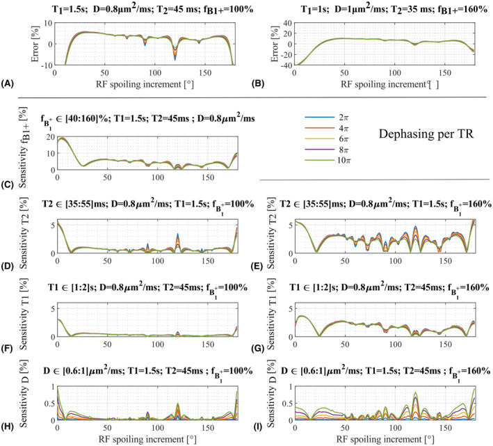
Numerical simulations, for each spoiling condition, of ${\mathrm{T}}_1^{\text{app}}$ error (ε) in two specific cases: T₁ = 1.5 s, D = 0.8 µm²/ms, T₂ = 45 ms, and ${\mathrm{f}}_{{\mathrm{B}}_1^{+}}$ = 100% (A); T₁ = 1 s, D = 1 µm²/ms, T₂ = 35 ms, and ${\mathrm{f}}_{{\mathrm{B}}_1^{+}}$ = 160% (B). Sensitivity of ${\mathrm{T}}_1^{\text{app}}$ to ${\mathrm{B}}_1^{+}$ efficiency (C), the true T₂ time (D‐E), the true T₁ time (F‐G), and the diffusion coefficient (H‐I). The sensitivity to T₁, T₂, and D are computed in two conditions: ${\mathrm{B}}_1^{+}$ efficiency of 100% (D‐F‐H) or 160% (E‐G‐I)

Higher $f_{B_1^{+}}$ and D, coupled with shorter T₂ and T₁, required markedly different ϕ ₀ (26°, 118°, 123°, and 171°) for ${\mathrm{T}}_1^{\text{app}}$ to match the true T₁ (Figure 1B), although dependence on nPi was reduced. However, the error was larger with over‐estimation peaking at 10% with ϕ ₀ = 48°.

Overall, no ϕ ₀ and nPi combination provided accurate T₁ estimates for all tissue properties and ${\mathrm{B}}_1^{+}$ efficiencies. The impact of gradient spoiling on the error was variable across the different conditions simulated.

${\mathrm{T}}_1^{\text{app}}$ was most sensitive to $f_{B_1^{+}}$ (Figure 1C). The degree of sensitivity was highly dependent on ϕ ₀. It reached 6% for the commonly used value of 50°, but fell below 2% for 117° when T₂, T₁, and D were fixed to 45 ms, 1500 ms, and 0.8 µm²/ms, respectively.

Sensitivity to T₂ (and T₁) was markedly lower falling below 2% (and 1%) for most ϕ ₀ when $f_{B_1^{+}}$ was optimal (ie, 100%, Figure 1D,F) but increased to 4% (and 3%) when $f_{B_1^{+}}$ was 160% (Figure 1E,G).

${\mathrm{T}}_1^{\text{app}}$ was least sensitive to D over the range of values tested. With T₁ and T₂ of 1500 ms and 45 ms, respectively, the maximum sensitivity did not exceed 1%, even for high $f_{B_1^{+}}$ (Figure 1H,I). Higher nPi increased sensitivity to D.

For some ϕ ₀, the sensitivity to T₂, T₁ and $f_{B_1^{+}}$ decreased as nPi increased (eg, 110° and 85°), whereas for others the opposite was true (eg, 60° and 72°).

3.2. Simulated error in T₁: impact of correction parameters

Correction factors derived from numerical simulations with T₂ = 45 ms and D = 0.8 µm²/ms dramatically decreased the error in ${\mathrm{T}}_1^{\text{app}}$ (c.f. Figures 1A and 2 middle row). However, the amplitude of the residual error was amplified by high $f_{B_1^{+}}$ and depended on whether the T₂ used to derive the correction factors (45 ms) matched that of the simulation (Figure 2). For the commonly used ϕ ₀ of 50°, a discrepancy in T₂ of 10 ms coupled with $f_{B_1^{+}}$ = 160% had a residual error of 2.7%.

FIGURE 2.

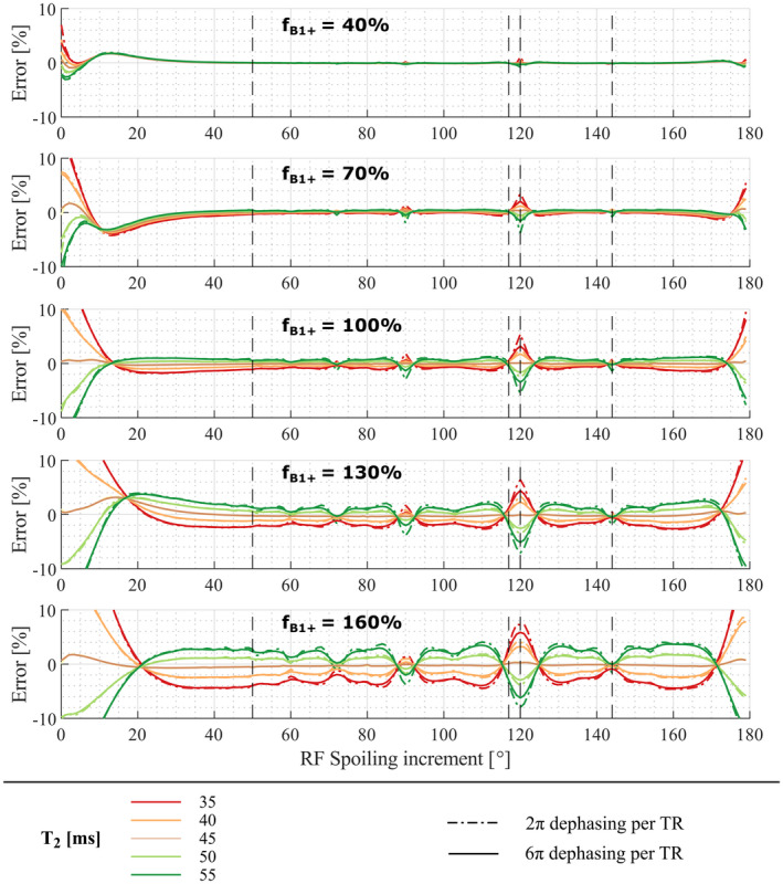
Residual errors after applying imperfect spoiling correction parameters derived with T₂ = 45 ms and D = 0.8 µm²/ms to ${\mathrm{T}}_1^{\text{app}}$. ${\mathrm{T}}_1^{\text{app}}$ was estimated from data simulated with a true T₁ time of 1.5 s, and a true T₂ time ranging from 35 to 55 ms for nPi = 2π (dashed lines) or 6π (solid lines). Each row corresponds to a different ${\mathrm{B}}_1^{+}$ efficiency, ${\mathrm{f}}_{{\mathrm{B}}_1^{+}}$, ranging from 40 to 160%. The error is minimized when the T₂ used to estimate the correction parameters matches the true T₂ (ie, 45 ms). Dashed vertical lines indicate the RF spoiling increments used in the in vivo acquisitions (ie, 50°, 117°, 120°,and 144°)

Some RF spoiling increments were more robust to the choice of T₂ and had lower residual error that further decreased by increasing the spoiler gradient moment. For the optimal combination of ϕ ₀ = 144° and nPi = 6π the correction parameters reduced the error to less than 0.8% for the full range of parameters investigated (Figure 2).

The particularly low T₂ sensitivity of 144° motivated its use in subsequent experiments. 120° was additionally investigated because of its comparatively high sensitivity to all parameters. 50° and 117° were selected because they are the most commonly encountered increments.

3.3. Comparison between simulation and phantom experiment

Reference T₂, T₁ and ADC values in the phantom were estimated to be 78 ± 2 ms, 952 ± 14 ms and 1.71 ± 0.04 μm²/ms, respectively.

The $f_{B_1^{+}}$ dependence of ${\mathrm{T}}_1^{\text{app}}$ (Figure 3A,B,F,G) matched the numerical simulations. ${\mathrm{T}}_1^{\text{app}}$ increased with $f_{B_1^{+}}$ for 50° (+ 50 ms) but decreased for 120° (−96 ms), and 117° (−77 ms), while 144° showed least sensitivity (−30 ms). The $f_{B_1^{+}}$ dependence of the increments of 120° and 144° was impacted by the increase of the spoiler gradient moment, whereas it had no observable impact for 117° and 50°.

FIGURE 3.

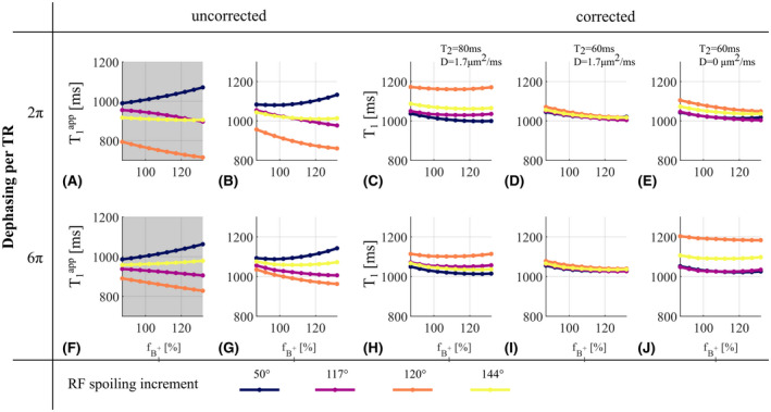
${\mathrm{T}}_1^{\text{app}}$ (A,B,F,G) and corrected T₁ (C,D,E,H,I,J) in the phantom with ${\varphi }_0\in {\left[50,117,120,144\right]}^{\circ }$, as a function of the ${\mathrm{B}}_1^{+}$ efficiency, ${\mathrm{f}}_{{\mathrm{B}}_1^{+}}$. Dephasing across a voxel of 2π (A‐E) and 6π (F‐J) per TR are shown. A,F, Numerical simulations. Fixed parameters are: T₁ = 950 ms, T₂ = 80 ms, D = 1.7 µm²/ms. B‐E,G‐J, Acquisitions. Corrected T₁ with correction factors from set 1 (C,H), set 2 (D,I), and set 3 (E,J) from Table 1A

${\mathrm{T}}_1^{\text{app}}$ maps were corrected with three sets of correction factors. The maps corrected with a T₂ of 80 ms showed almost no $f_{B_1^{+}}$ dependence but had a ϕ ₀‐dependent offset (Figure 3C,H)_, which was removed when T₂ was reduced to 60 ms (Figure 3D,I). However, when the correction factors were computed without accounting for diffusion, the corrected T₁ again showed ϕ ₀‐dependent offsets_, particularly with a large spoiler gradient moment (Figure 3E,J).

3.4. Comparison between simulation and in vivo experiment

Reference T₂, T₁ and ADC value in the WM region used for subsequent analyses were estimated to be 47 ± 6 ms, 1260 ± 50 ms and 0.7 ± 0.1 µm²/ms, respectively.

The dependence of ${\mathrm{T}}_1^{\text{app}}$ on $f_{B_1^{+}}$ (Figure 4A,C) predicted by simulation was observed in vivo (Figure 4B,D). ϕ ₀ of 50° and 120° were most sensitive to $f_{B_1^{+}}$ with ${\mathrm{T}}_1^{\text{app}}$ varying by +41 ms or −40 ms, respectively, between 65 and 110% efficiency. The variation was 24 ms for 117° and 5 ms for 144°. As predicted, increasing the gradient spoiler moment had the biggest impact on 120°, for which the ${\mathrm{T}}_1^{\text{app}}$ variation decreased to −15 ms over the range of $f_{B_1^{+}}$.

FIGURE 4.

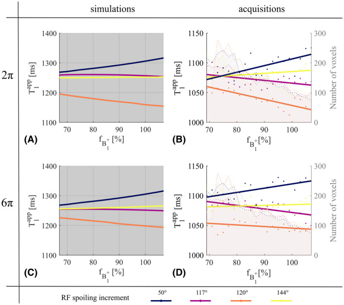
In vivo${\mathrm{T}}_1^{\text{app}}$, obtained with ${\varphi }_0\in {\left[50,117,120,144\right]}^{\circ }$, as a function of the ${\mathrm{B}}_1^{+}$ efficiency, ${\mathrm{f}}_{{\mathrm{B}}_1^{+}}$. Dephasing across a voxel of 2π (A,B) and 6π (C,D) per TR are shown. A,C, Numerical simulations. Fixed parameters are: T₁ = 1250 ms, T₂ = 45 ms, D = 0.8 µm²/ms. B,D, Acquisitions, and linear fitting for illustration purposes. The number of voxels included in each bin is depicted by the shaded background of each graph for each ϕ₀

Simulations predicted that, as T₂ increased, ${\mathrm{T}}_1^{\text{app}}$ would be under‐estimated for ϕ ₀ = 120° or slightly over‐estimated for ϕ ₀ = 50° (Figure 5). A small T₂‐dependence was predicted for 117° and even less so for 144°. These dependencies were predicted to be accentuated when $f_{B_1^{+}}$ increased to 130% and to be reduced when nPi was increased from 2π to 6π. Most of those predictions were observed in vivo: over the T₂ range, with 2π gradient spoiling, ${\mathrm{T}}_1^{\text{app}}$ decreased by 51 ms for 120° and increased by 30 ms for 50°. This reduced to 12 and 25 ms, respectively, for 6π. The variation of ${\mathrm{T}}_1^{\text{app}}$ for 117° and 144° did not exceed 20 ms. Discrepancies between simulations and acquisitions occurred in the case of high $f_{B_1^{+}}$ and gradient spoiling (Figure 5H). ${\mathrm{T}}_1^{\text{app}}$ showed the predicted reduction with increasing T₂ for 120°, but an unpredicted offset. An unpredicted increase was also observed for 144° while the increased T₂‐dependence predicted for 50° was not observed (Figure 5D,H).

FIGURE 5.

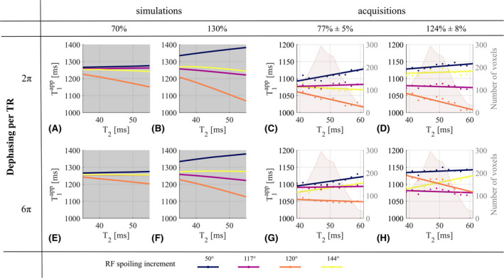
In vivo${\mathrm{T}}_1^{\text{app}}$, obtained with ${\varphi }_0\in {\left[50,117,120,144\right]}^{\circ }$, as a function of T₂. Dephasing across a voxel of 2π (A‐D) and 6π (E‐H) per TR are shown. Original (×1) (A,C,E,G) and high (×1.6) (B,D,F,H) transmitter reference voltage are shown. A,B,E,F, Numerical simulations. Fixed parameters are: T₁ = 1250 ms, D = 0.8 µm²/ms, ${\mathrm{f}}_{{\mathrm{B}}_1^{+}}=70\text{\%}$, and 130% as measured in the transmit field map in the slice of interest. C,D,G,H, Acquisitions, and linear fitting for illustration purposes. The number of voxels included in each bin is depicted by the shaded background of each graph for each ϕ₀

3.5. Impact of correction parameters in vivo

Although the T₁ maps with different spoiling conditions, with and without correction for imperfect spoiling, were qualitatively similar (Figure 6), some distinct contrast differences were observed, for example, between GM and cerebrospinal fluid (green box) and within the basal ganglia (black box). The within‐increment SD (σ_row ) across T₁ maps revealed particularly high sensitivity to spoiling condition and the T₂ used to derive the correction parameters (c.f. Figure 6B ϕ ₀ of 50° or 120° versus 117° or 144°). The T₁ maps converged (low σ_col , Figure 6C) when sufficient gradient spoiling (nPi = 6π) was combined with a T₂ of 35 ms to derive the correction parameters, but diverged (high σ_col , Figure 6C) when low spoiling (nPi = 2π) was combined with no correction for imperfect spoiling or one based on a T₂ of 55 ms.

FIGURE 6.

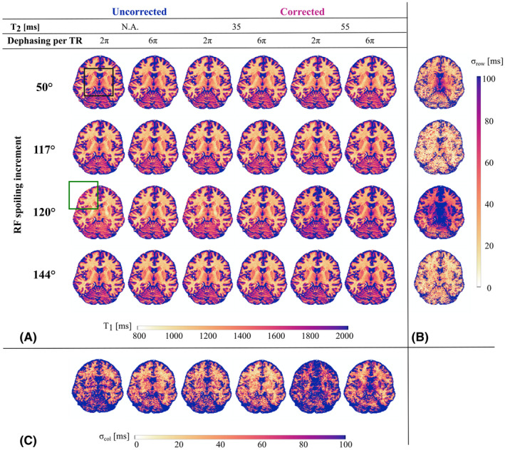
A, Axial view from T₁ maps obtained with nominal ${\mathrm{f}}_{{\mathrm{B}}_1^{+}}$ (ie, no reference voltage manipulation) and nPi = 2π (columns 1, 3, and 5) or 6π (columns 2, 4, and 6) for each RF spoiling increment (rows). These are presented before (ie, ${\mathrm{T}}_1^{\text{app}}$, columns 1 and 2) and after correction for imperfect spoiling using a fixed D of 0.8 µm²/ms and a T₂ of either 35 ms (columns 3 and 4) or 55 ms (columns 5 and 6). Black and green boxes highlight areas particularly affected by changing nPi or applying correction factors. B, Maps of σ _row, the voxel‐wise SD of T₁ across conditions for a given RF spoiling increment (ie, along rows in (A)). C, Maps of σ_col, the voxel‐wise SD of T₁ across RF spoiling increments for a given condition (ie, along columns in (A))

The impact of correcting for imperfect spoiling increased with $f_{B_1^{+}}$ (Figure 7). The correction induced the largest shifts in T₁ for ϕ ₀ of 50° (Figure 7), especially when $f_{B_1^{+}}$ = 160%. The higher variance observed across conditions for this increment (Figure 6B) also exhibits a pattern consistent with the $f_{B_1^{+}}$ profile. ϕ ₀ = 117° only benefited from correction at high $f_{B_1^{+}}$.

FIGURE 7.

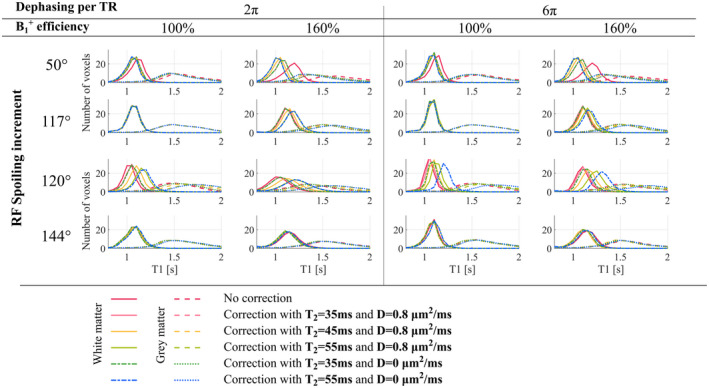
Histograms of the estimated T₁ times for WM and GM without (ie, ${\mathrm{T}}_1^{\text{app}}$) and with correction for imperfect spoiling. Five sets of correction factors were computed based on different T₂ times and diffusion coefficients and applied separately. Only those voxels with ${\mathrm{f}}_{{\mathrm{B}}_1^{+}}$ between 95% and 105% (measured with no reference voltage manipulation) were included in the analysis

Corrected T₁ times were highly dependent on the T₂ used for the correction, especially when $f_{B_1^{+}}$ was 160%. A global T₂ time of 35 ms minimized dependence on ϕ ₀ (Figure 6C). ϕ ₀ = 120° was additionally dependent on D regardless of experimental conditions. ϕ ₀ = 144° was exceptional in that the corrected T₁ times were effectively independent of the tissue properties (T₂ and D) used to determine the correction parameters.

3.6. Artifact dependence on spoiling conditions

The weighted images used to calculate T₁ were affected by background artifacts when nPi = 2π (Figure 8A). With rectangular k‐space sampling, the artifact manifested as a coherent alias of brain edges. Its location depended on ϕ ₀: the replica was shifted in the partition direction for 117°, but in both the partition and line directions for 50°. While still visible, the artifact was more diffuse with elliptical sampling (Figure 8A). Numerical simulations with rectangular k‐space sampling based on a mixed population of isochromats (different resonance frequencies) showed phase variation across TR (Figure 8C). ϕ ₀ = 117° produced a periodic phase variation across partitions consistent with the observed position of the ghost artifact in the field‐of‐view along this direction. ϕ ₀ = 50° resulted in phase variation in both the lines and partitions directions, again consistent with the empirical data.

FIGURE 8.

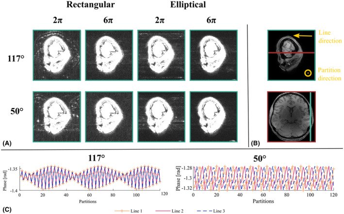
A, Sagittal view of T₁‐weighted images acquired with rectangular or elliptical k‐space sampling using different spoiling conditions. The images have been windowed to highlight background signal. B, The same sagittal slice and an axial slice are shown windowed to visualize the brain. The turquoise line in the axial view indicates the sagittal position while the red line on the sagittal view indicates the axial position. The two phase‐encoding directions (lines and partitions) are indicated in the sagittal view. C, Numerical simulations of the impact of partial voluming on the phase of the signal across lines and partitions (rectangular sampling case, all partitions are acquired before incrementing the line) for each RF spoiling increment

4. DISCUSSION

We have demonstrated a complex relationship between the estimated T₁ and the spoiling regime within the context of the 3D VFA approach. Our simulations (Figure 1) indicate that no RF spoiling increment would lead to ${\mathrm{T}}_1^{\text{app}}$ matching the true T₁ across all conditions (ie, sequence choices, T₂ times, and diffusion coefficients). Furthermore, the simulations show that even the fullest effects of diffusion achieved in a multi‐echo acquisition are insufficient to achieve perfect spoiling of the transverse magnetisation.

The sensitivity to imperfect spoiling effects will depend on the specifics of the protocol used. It has recently been suggested that the maximum flip angle should be minimized to mitigate spoiling‐induced errors.³⁷ However, for the TR and target T₁ range considered here, this would compromise the precision of the T₁ estimates by as much as 50%.³⁸ An alternative would be to reduce both flip angles and TR, which could be achieved by adopting a single echo protocol. However, simulations suggest that the sensitivity of such an approach would be on a par with that observed in the protocol used here (c.f. Figure 1 and Supporting Information Figure S2). Combining a single echo approach with a long TR and using the time to impart extensive gradient spoiling is predicted to reduce the sensitivity of T₁ estimates to imperfect spoiling, even in the case of high flip angles (Supporting Information Figure S2). However, unlike the multi‐echo MPM protocol adopted here, single echo protocols prevent ${\mathrm{T}}_2^{\ast }$ from being concurrently estimated, and prevent extrapolation to TE = 0 ms, which aims to remove bias introduced by flip angle‐dependent ${\mathrm{T}}_2^{\ast }$ decay³⁵, ³⁹ from the T₁ estimates. Slice‐selective 2D acquisitions would naturally achieve a long TR and improved spoiling behaviour, but suffer limitations such as MT effects and imperfect slice profiles that lead to flip angle‐dependent⁴⁰ bias in the T₁ estimates.

In the context of the MPM protocol investigated here ${\mathrm{T}}_1^{\text{app}}$ was most sensitive to $f_{B_1^{+}}$, which could lead to over‐estimation of the true T₁ by as much as 30%. Despite accounting for $f_{B_1^{+}}$ inhomogeneity in both simulations and acquisitions (Equation 1), ${\mathrm{T}}_1^{\text{app}}$ continued to depend on $f_{B_1^{+}}$ in an increment‐specific manner. Some ϕ ₀, such as the commonly used 50°, were particularly sensitive (Figures 1,3 and 4), although the error can be markedly reduced by post‐hoc correction for imperfect spoiling (Figures 2,3 and 6). Since the correction factors are a function of both ${\mathrm{T}}_1^{\text{app}}$ and $f_{B_1^{+}}$ (Equation 3), they rely on accurate estimation of the true $f_{B_1^{+}}$. Any error will propagate through to the corrected T₁ time. It may then be appealing to select a ϕ ₀ that exhibits lower sensitivity to $f_{B_1^{+}}$, for example, 117° or 144° (Figures 1 and 3). However, the sensitivity of ${\mathrm{T}}_1^{\text{app}}$ to inaccurate or imprecise definition of the flip angles ($f_{B_1^{+}}$ in Equation 1) would remain.⁴¹

Other sources of $f_{B_1^{+}}$ dependence may affect the accuracy of the T₁ estimate, and were reduced as much as possible in this work:

1. MT effects, proportional to the square of the amplitude of the transmit field, have been shown to bias ${\mathrm{T}}_1^{\text{app}}$ ³⁷, ⁴², ⁴³ and can be expected to be a more significant problem at 7T. Experimentally, the MT effect was limited by the use of rectangular pulses with matched power for the PD‐ and T₁‐weighted acquisitions. Nonetheless, residual dependence may remain and may underlie the offset between the T₁ measured in WM with the IR‐SE‐EPI (1260 ms) and VFA (~1100 ms) approaches. MT effects were not included in any of our simulations of the steady‐state signal since it depends on a number of unknown, spatially varying tissue properties. However, we can estimate the impact of MT effects in the present context for WM using the EPG‐X framework (https://github.com/mriphysics/EPG‐X).⁴⁴, ⁴⁵ Assuming a bound pool fraction (BPF) of 0.117,⁴⁴ thermal equilibrium with an exchange rate from free to bound pool of 4.3 s⁻¹,⁴⁴ and a T₁ time of 1.25 s for each pool, the MT effect caused ${\mathrm{T}}_1^{\text{app}}$ to decrease as $f_{B_1^{+}}$ increased. Depending on the RF spoiling increment used, this bias could either counteract (eg, ϕ ₀ = 50°) or accentuate (eg, ϕ ₀ = 120°) the $f_{B_1^{+}}$ sensitivity induced by imperfect spoiling (Figure 9B). However, the MT effect was largely independent of the RF spoiling increment (Figure 9A). A method has recently been proposed to counteract MT effects at the time of acquisition.⁴³

2. ${\mathrm{T}}_2^{\ast }$ has previously been shown to depend on the excitation flip angle.³⁵ If differential ${\mathrm{T}}_2^{\ast }$ weighting exists in the SPGR signals Equation (1) will lead to biased T₁ estimates. Unlike single echo approaches, the multi‐echo approach adopted here allows extrapolation to TE = 0 ms to limit this source of $f_{B_1^{+}}$‐dependent bias.

3. The approximations implemented by default in the hMRI toolbox offer flexibility but introduce $f_{B_1^{+}}$‐dependent bias when the assumptions are violated at higher flip angle.¹³ Matched TR across the SPGR acquisitions permitted ${\mathrm{T}}_1^{\text{app}}$ to be estimated without approximation¹⁴ circumventing this potential source of bias.

FIGURE 9.

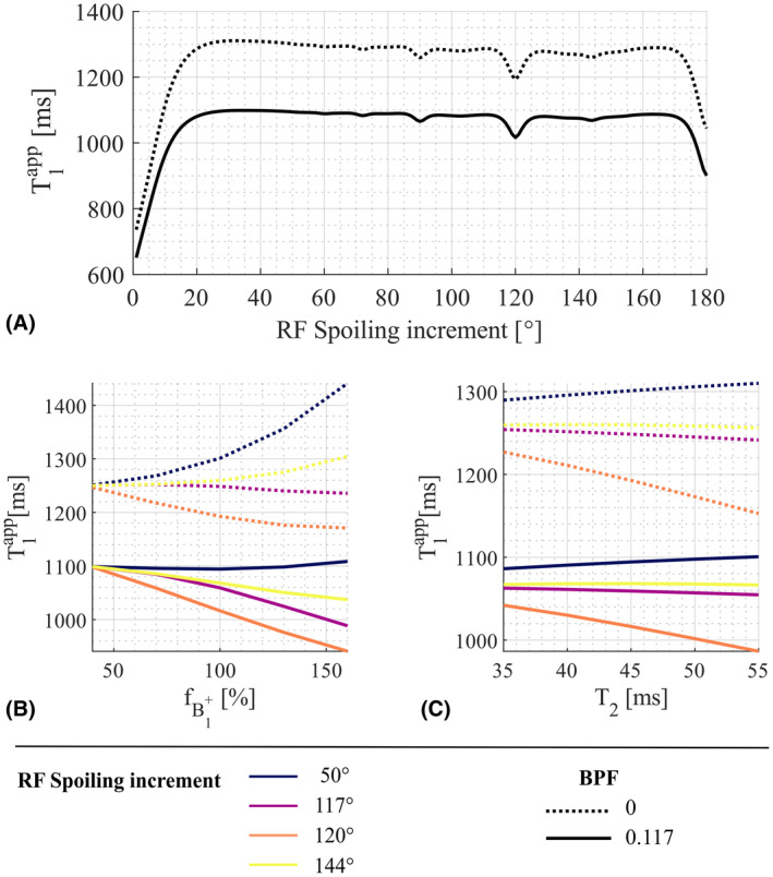
Numerical simulations without (BPF = 0, dashed line) and with (BPF = 0.117, solid line) a bound pool fraction leading to MT. The exchange rate from the free to the bound pool was 4.3 s⁻¹,⁴⁴ and thermal equilibrium was assumed. The BPF was 0.117⁴⁴ and the diffusion coefficient was 0.8 µm²/ms. A, ${\mathrm{T}}_1^{\text{app}}$ for ϕ ₀ from 1 to 180°, T₂ = 45 ms, T₁ = 1.25 s (for both pools), and ${\mathrm{f}}_{{\mathrm{B}}_1^{+}}$ of 100%. The total dephasing per TR was set to 6π. B‐C, ${\mathrm{T}}_1^{\text{app}}$ as a function of ${\mathrm{f}}_{{\mathrm{B}}_1^{+}}$ and T₂ time, respectively, for ϕ ₀ = 50°, 117°, 120°, and 144°

At 7T, T₂ shortens increasing the feasibility of fully spoiling the transverse magnetisation. Any T₂‐dependence is an important consideration since it can lead to spatially varying, microstructurally driven error in T₁ estimation. Both simulation and experiment showed that some RF spoiling increments are particularly sensitive to T₂ (Figure 5) and that the error increases in regions of high $f_{B_1^{+}}$. Analysis of the EPGs can provide some insights into these observations (Supporting Information S4, Supporting Information Figures S5 and S6). However, incorporating knowledge of T₂ to correct this error is difficult since accurate quantification is challenging and time‐consuming, particularly at high resolution, and can also depend on factors like $f_{B_1^{+}}$ and slice profiles.⁴⁶, ⁴⁷ Here, we have observed the T₂‐dependence of ${\mathrm{T}}_1^{\text{app}}$ by measuring T₂ with a single‐echo spin‐echo EPI technique to maximise accuracy and minimize confounding factors. The choice of T₂ used to derive the correction factors is particularly important for the commonly used ϕ ₀ = 50°, which exhibits higher T₂ sensitivity (Figures 3, 6, and 7). Although the post‐hoc correction for imperfect spoiling is not voxel‐specific, global T₂ times of 35 ms in vivo and 60 ms in phantom, resulted in the convergence of the corrected T₁ distributions regardless of their acquisition conditions (Figures 3, 6, and 7). However, these T₂ times were smaller than literature values for in vivo WM at 7T²⁸ and those estimated with the reference protocol (T₂ of 48 ± 6 ms and 78 ± 2 ms in vivo and in phantom, respectively). Note that using an array of T₂ times to match those expected in vivo will have the same compromise effect whereby error may increase or decrease depending on the true T₂.

The issue of T₂‐dependence in the estimated T₁, including after correction, has been highlighted previously at 3T.¹², ¹⁹ The manifestation of imperfect spoiling at 3T differs to 7T most notably by a greater dependence on the gradient spoiling and diffusional effects at 3T (see Supporting Information Figures S3 and S4 for a 3T analysis). Baudrexel et al¹⁹ proposed an alternative correction method to the one used here, which adjusts the flip angle to account for imperfect spoiling before estimating T₁. The T₂‐dependence of that technique was not compared to the method used here, but in phantoms with variable T₂, showed a residual deviation of 1 to 3%. As an alternative to estimating T₁ using an analytical solution of the Ernst equation, Heule et al¹² proposed a numerical minimization approach that does not rely on perfect spoiling. The approach performed well in comparison to the correction technique adopted here, particularly in terms of reducing theoretical sensitivity to T₂. However, the residual error increased with the diffusion coefficient and the moment of the spoiler gradient. Here, we have shown that a large spoiler moment is beneficial not only to reduce ${\mathrm{T}}_1^{\text{app}}$ sensitivities, but also to minimize artifacts due to partial voluming (Figure 8). The ghost artifacts we observed, and explained by numerical simulation, are another consequence of imperfect spoiling previously highlighted by Nielsen and Noll³¹ and an important consideration when designing a protocol.

At 7T, simulations incorporating the diffusion effect, due to both the multi‐echo readout and the spoiler gradient, demonstrated a detectable effect on ${\mathrm{T}}_1^{\text{app}}$ when using in vivo T₂ times and clinically feasible spoiler moments. In phantom, where the ADC was estimated to be 1.71 µm²/ms, the sensitivity to $f_{B_1^{+}}$ depended on the spoiler gradient moment, and it was necessary to include the diffusion effect when determining the correction factors to obtain consistent ${\mathrm{T}}_1^{\text{app}}$ across φ₀, especially for the large spoiler gradient condition. In healthy in vivo tissue, the estimated ADC was lower (0.7 µm²/ms) in line with literature.²⁹, ³⁰ The sensitivity to this parameter over the range of likely values was generally small (<1%), even for nPi = 6π, which required a net moment of 70.5 mT/m.ms at 1 mm resolution. Nonetheless, the effect of diffusion was observed in vivo and the T₂‐dependence was reduced for ϕ ₀ of 50° and 120°, when nPi was increased to 6π, in line with the simulations. Including the diffusion effect in the correction factors only had an appreciable impact with φ₀ = 120°. However, the higher the spoiler gradient moment, the higher the expected sensitivity to the diffusion coefficient (Figures 1I, Supporting Information Figures S2 and S3I).

RF spoiling increments of 50° and 117° are commonly used. 50° has the advantage of being located in a stable region¹⁷ but, as shown here, may not be the most suitable because of its high sensitivity to $f_{B_1^{+}}$ and T₂. 117° is known for being close to perfect spoiling conditions. However, it is shown here that despite reducing ${\mathrm{T}}_1^{\text{app}}$ error, residual T₂‐dependence remains, especially at high $f_{B_1^{+}}$. ϕ ₀ = 144° shows appealing robustness to T₂ with clinically feasible spoiler moments, making it a good candidate for VFA‐based T₁ measurements. However, a broader histogram (Figure 7) and larger than predicted T₂‐dependence (Figure 5E‐H) were measured in vivo for this increment, meaning that we cannot exclude the possibility that it may be a less stable choice.¹⁷

4.1. Limitations

Although efforts were made to remove confounding effects, such as anatomical variability, some discrepancies were observed between simulations and experiments (Figure 5). In addition to the issue of MT effects discussed earlier, the observed discrepancies may come from residual variance in T₁ or diffusion properties, or other microstructural features not well modeled by single pool simulations, for example, myelin water.

Some further limitations warrant discussion. This work has been performed at 7T using only a small number of protocols with many fixed parameters, for example, resolution, TR and number of echoes. Nonetheless, good agreement was observed between simulations and acquisitions indicating that the same framework could be used to investigate other protocols.

The resolution used is relatively low for 7T imaging (1 mm isotropic) but was required to maintain a tolerable scan time per session given the number of factors probed ($f_{B_1^{+}}$, nPi, ϕ ₀). With high resolution, the diffusion effect can be expected to increase due to the larger moment of the readout gradients, while the risk of partial voluming will concurrently reduce.

The sensitivity of ${\mathrm{T}}_1^{\text{app}}$ to each of the sequence parameters and tissue properties was investigated for a limited range of values. However, these were selected to encompass the range expected in the context of neuroimaging at 7T. The sensitivity may increase in pathology, but again the validated framework presented here could be used to determine optimal protocol strategies.

5. CONCLUSIONS

We conclude by returning to the questions posed in the introduction:

• 1How do RF and gradient spoiling interact and which combination maximizes the accuracy and precision of T₁ mapping with the VFA approach?

The interaction between RF and gradient spoiling is complex. The error in ${\mathrm{T}}_1^{\text{app}}$ depends not only on ϕ ₀, but also on $f_{B_1^{+}}$ and T₂ times, as does its sensitivity. The impact that gradient spoiling has on the error and sensitivity also depends on ϕ ₀. Increasing the net gradient‐induced dephasing per TR reduces the dependence on ϕ ₀, except in terms of sensitivity to the diffusion coefficient (Figure 1). Since no combination achieves perfect spoiling, the preferred approach may be to maximise the robustness of ${\mathrm{T}}_1^{\text{app}}$ to other parameters that are fixed in post‐hoc correction, principally T₂. Larger spoiler gradient moment has the additional benefit of improving image quality.

• 2What impact does the diffusion effect have when considering clinically feasible gradient moments and the impact of the full readout?

Including the full diffusion effect of a multi‐echo readout has a comparatively small impact at 7T relative to 3T for healthy tissues (Supporting Information Figures S3 and S4). Correction factors accounting for diffusion are especially important at lower field strengths due to longer T₂ or in pathology for higher diffusion coefficient, and can now be estimated via the hMRI toolbox (hmri.info²⁰).

• 3What are the limitations of applying simulation‐derived correction factors to recover the true T₁ from ${\mathrm{T}}_1^{\text{app}}$?

The main limitation of post‐hoc correction is the need to specify a single T₂ time, leading to residual T₂‐dependence. Combining ϕ ₀ = 144° with moderate gradient spoiling minimizes the sensitivity of ${\mathrm{T}}_1^{\text{app}}$ to T₂.

Supporting information

FIGURE S1 (A) Positioning of the slices used to obtain reference T₁ (B,E) and T₂ (C,F) times using single slice, single echo, spin echo EPI acquisitions. Reference ADC estimates (D,G) from the same slices are also shown. The more superior slice (yellow) had lower $f_{B_1^{+}}$ variance and was therefore used to investigate the T₂ dependence. The more inferior slice (red) had greater $f_{B_1^{+}}$ variance and was therefore used to investigate the $f_{B_1^{+}}$ dependence

FIGURE S2 Sensitivity of ${\mathrm{T}}_1^{\text{app}}$ to ${\mathrm{B}}_1^{+}$ efficiency (A), the true T₂ time (B,C), the true T₁ time (D,E) and the diffusion coefficient (F‐G) of three single‐echo protocols: Protocol 1 (blue), 2 (red) and 3 (yellow). The sensitivity to T₁, T₂ and D are computed in two conditions: ${\mathrm{B}}_1^{+}$ efficiency of 100% or 160%

FIGURE S3 Numerical simulations, for each spoiling condition, of ${\mathrm{T}}_1^{\text{app}}$ error in two specific cases: (A) T₁ = 1250 ms, D = 0.8 µm²/ms, T₂ = 65 ms and $f_{B_1^{+}}$ = 100%, (B) T₁ = 0.75 s, D = 1.0 µm²/ms, T₂ = 55 ms and $f_{B_1^{+}}$ = 130%. Sensitivity of ${\mathrm{T}}_1^{\text{app}}$ to $f_{B_1^{+}}$ (C), the true T₂ time (D‐E), the true T₁ time (F‐G) and the true diffusion coefficient (H‐I). The sensitivity to T₁, T₂ and D are computed in two conditions: ${\mathrm{B}}_1^{+}$ efficiency of 100 % (D‐F‐H) or 130 % (E‐G‐I)

FIGURE S4 Acquisitions and numerical simulations at 3T for RF spoiling increments of 30°, 72°, 117°, 120° and 137°. T₁ before (ie, ${\mathrm{T}}_1^{\text{app}}$) and after correction for imperfect spoiling with correction factors determined assuming T₂ = 65 ms and D = 0.8 µm²/ms or ignoring diffusion. Simulations (left): true T₁ times are indicated by a solid black line at 1 s and 1.5 s. In vivo acquisitions (right): distribution of T₁ times in GM and WM where ${\mathrm{B}}_1^{+}$ efficiency was between 90% and 110%

FIGURE S5 EPG diagrams, before (A, C) and after (B, D) incorporating diffusion. The diagrams depict the population amplitude of transverse, $\left|F_n\right|$ and longitudinal, $\left|Z_n\right|$, configuration states with n the degree of dephasing $\varphi =2\pi$. The simulations used a T₁ of 1000 ms, T₂ of 80 ms and a diffusion coefficient of 1.7 μm²/s with a flip angle of 6° and a TR of 19.5 ms. Note that for visualisation purposes only a subset of the EPG diagrams are shown: 0 < n ≤ 20 for the dephasing transverse configuration states, 0 > n ≥ −20 for the rephasing transverse magnetization and 0 ≤ n ≤ 40 for the longitudinal states. Higher order longitudinal and rephasing states are more populated for the RF spoiling increments of 120° and 144°. Since higher order states are especially attenuated by diffusion, incorporating this effect has the most appreciable impact on these increments. It can also be seen that sufficient pulses are incorporated to reach a steady state, which is arrived at comparatively quickly for all increments

FIGURE S6 Intra‐voxel magnetisation distribution derived from the steady‐state EPG coefficients for each increment (A), and the population amplitudes of the first six rephasing transverse configuration states (B). Four cases are shown: two nominal flip angles (6° and 26° corresponding to the PDw and T1w acquisitions of this study) and two T₂ times (60 ms and 80 ms). All other simulation settings are as in Supporting Information Figure S5. The net SPGR echo‐forming signal (ie, $F_0$ state) is projected onto the transverse plane in (A) with an artificial phase dispersion added to aid visualisation

Corbin N, Callaghan MF. Imperfect spoiling in variable flip angle T₁ mapping at 7T: Quantifying and minimizing impact. Magn Reson Med. 2021;86:693–708. 10.1002/mrm.28720

REFERENCES

- 1.Weiskopf N, Mohammadi S, Lutti A, Callaghan M. Advances in MRI‐based computational neuroanatomy: from morphometry to in‐vivo histology. Curr Opin Neurol. 2015;28:313‐322. [DOI] [PubMed] [Google Scholar]
- 2.Edwards LJ, Kirilina E, Mohammadi S, Weiskopf N. Microstructural imaging of human neocortex in vivo. Neuroimage. 2018;182:184‐206. [DOI] [PubMed] [Google Scholar]
- 3.Lutti A, Dick F, Sereno MI, Weiskopf N. Using high‐resolution quantitative mapping of R1 as an index of cortical myelination. Neuroimage. 2014;93:176‐188. [DOI] [PubMed] [Google Scholar]
- 4.Sereno MI, Lutti A, Weiskopf N, Dick F. Mapping the human cortical surface by combining quantitative T1 with retinotopy. Cereb Cortex. 2013;23:2261‐2268. [DOI] [PMC free article] [PubMed] [Google Scholar]
- 5.Carey D, Krishnan S, Callaghan MF, Sereno MI, Dick F. Functional and quantitative MRI mapping of somatomotor representations of human supralaryngeal vocal tract. Cereb Cortex. 2017;27:265‐278. [DOI] [PMC free article] [PubMed] [Google Scholar]
- 6.Dick FK, Lehet MI, Callaghan MF, Keller TA, Sereno MI, Holt LL. Extensive tonotopic mapping across auditory cortex is recapitulated by spectrally directed attention and systematically related to cortical myeloarchitecture. J Neurosci. 2017;37:12187‐12201. [DOI] [PMC free article] [PubMed] [Google Scholar]
- 7.Dick F, Tierney AT, Lutti A, Josephs O, Sereno MI, Weiskopf N. In vivo functional and myeloarchitectonic mapping of human primary auditory areas. J Neurosci. 2012;32:16095‐16105. [DOI] [PMC free article] [PubMed] [Google Scholar]
- 8.Christensen K, Grant D, Schulman E, Walling C. Optimal determination of relaxation‐times of Fourier‐transform nuclear magnetic‐resonance ‐ determination of spin‐lattice relaxation‐times in chemically polarized species. J Phys Chem. 1974;78:1971‐1977. [Google Scholar]
- 9.Wang H, Riederer S, Lee J. Optimizing the precision in T1 relaxation estimation using limited flip angles. Magn Reson Med. 1987;5:399‐416. [DOI] [PubMed] [Google Scholar]
- 10.Homer J, Beevers MS. Driven‐equilibrium single‐pulse observation of T1 relaxation. A reevaluation of a rapid “new” method for determining NMR spin‐lattice relaxation times. J Magn Reson (1969). 1985;63:287‐297. [Google Scholar]
- 11.Deoni SCL, Rutt BK, Peters TM. Rapid combined T‐1 and T‐2 mapping using gradient recalled acquisition in the steady state. Magn Reson Med. 2003;49:515‐526. [DOI] [PubMed] [Google Scholar]
- 12.Heule R, Ganter C, Bieri O. Variable flip angle T1 mapping in the human brain with reduced t2 sensitivity using fast radiofrequency‐spoiled gradient echo imaging. Magn Reson Med. 2016;75:1413‐1422. [DOI] [PubMed] [Google Scholar]
- 13.Helms G, Dathe H, Dechent P. Quantitative FLASH MRI at 3T using a rational approximation of the Ernst equation. Magn Reson Med. 2008;59:667‐672. [DOI] [PubMed] [Google Scholar]
- 14.Mohammadi S, D’Alonzo C, Ruthotto L, et al. Simultaneous adaptive smoothing of relaxometry and quantitative magnetization transfer mapping. 2017. 10.20347/WIAS.PREPRINT.2432 [DOI]
- 15.Ganter C. Steady state of gradient echo sequences with radiofrequency phase cycling: analytical solution, contrast enhancement with partial spoiling. Magn Reson Med. 2006;55:98‐107. [DOI] [PubMed] [Google Scholar]
- 16.Zur Y, Wood ML, Neuringer LJ. Spoiling of transverse magnetization in steady‐state sequences. Magn Reson Med. 1991;21:251‐263. [DOI] [PubMed] [Google Scholar]
- 17.Preibisch C, Deichmann R. Influence of RF spoiling on the stability and accuracy of T1 mapping based on spoiled FLASH with varying flip angles. Magn Reson Med. 2009;61:125‐135. [DOI] [PubMed] [Google Scholar]
- 18.Yarnykh VL. Optimal radiofrequency and gradient spoiling for improved accuracy of T1 and B1 measurements using fast steady‐state techniques. Magn Reson Med. 2010;63:1610‐1626. [DOI] [PubMed] [Google Scholar]
- 19.Baudrexel S, Nöth U, Schüre J‐R, Deichmann R. T1 mapping with the variable flip angle technique: a simple correction for insufficient spoiling of transverse magnetization. Magn Reson Med. 2018;79:3082‐3092. [DOI] [PubMed] [Google Scholar]
- 20.Tabelow K, Balteau E, Ashburner J, et al. hMRI—a toolbox for quantitative MRI in neuroscience and clinical research. Neuroimage. 2019;194:191‐210. [DOI] [PMC free article] [PubMed] [Google Scholar]
- 21.Callaghan MF, Lutti A, Ashburner J, et al. Example dataset for the hMRI toolbox. Data Brief. 2019;25:104132. [DOI] [PMC free article] [PubMed] [Google Scholar]
- 22.Lamy J, Loureiro de Sousa P. Sycomore: an MRI simulation toolkit. In: ISMRM. Virtual; 2020. p 2072.
- 23.Weigel M, Schwenk S, Kiselev VG, Scheffler K, Hennig J. Extended phase graphs with anisotropic diffusion. J Magn Reson. 2010;205:276‐285. [DOI] [PubMed] [Google Scholar]
- 24.Wright PJ, Mougin OE, Totman JJ, et al. Water proton T1 measurements in brain tissue at 7, 3, and 1.5T using IR‐EPI, IR‐TSE, and MPRAGE: results and optimization. Magn Reson Mater Phy. 2008;21:121‐130. [DOI] [PubMed] [Google Scholar]
- 25.Rooney WD, Johnson G, Li X, et al. Magnetic field and tissue dependencies of human brain longitudinal 1H2O relaxation in vivo. Magn Reson Med. 2007;57:308‐318. [DOI] [PubMed] [Google Scholar]
- 26.Metere R, Kober T, Möller HE, Schäfer A. Simultaneous Quantitative MRI mapping of T1, T2* and magnetic susceptibility with multi‐echo MP2RAGE. PLoS One. 2017;12:e0169265. [DOI] [PMC free article] [PubMed] [Google Scholar]
- 27.Marques JP, Kober T, Krueger G, van der Zwaag W, Van de Moortele P‐F, Gruetter R. MP2RAGE, a self bias‐field corrected sequence for improved segmentation and T1‐mapping at high field. Neuroimage. 2010;49:1271‐1281. [DOI] [PubMed] [Google Scholar]
- 28.Cox EF, Gowland PA. Simultaneous quantification of T2 and T′2 using a combined gradient echo‐spin echo sequence at ultrahigh field. Magn Reson Med. 2010;64:1440‐1445. [DOI] [PubMed] [Google Scholar]
- 29.Helenius J, Soinne L, Perkiö J, et al. Diffusion‐weighted MR imaging in normal human brains in various age groups. Am J Neuroradiol. 2002;23:194‐199. [PMC free article] [PubMed] [Google Scholar]
- 30.Sener RN. Diffusion MRI: apparent diffusion coefficient (ADC) values in the normal brain and a classification of brain disorders based on ADC values. Comput Med Imaging Graph. 2001;25:299‐326. [DOI] [PubMed] [Google Scholar]
- 31.Nielsen J‐F, Noll DC. Improved spoiling efficiency in dynamic RF‐spoiled imaging by ghost phase modulation and temporal filtering. Magn Reson Med. 2016;75:2388‐2393. [DOI] [PMC free article] [PubMed] [Google Scholar]
- 32.Sacolick LI, Wiesinger F, Hancu I, Vogel MW. B1 Mapping by Bloch‐Siegert shift. Magn Reson Med. 2010;63:1315‐1322. [DOI] [PMC free article] [PubMed] [Google Scholar]
- 33.Hansen MS, Sørensen TS. Gadgetron: an open source framework for medical image reconstruction. Magn Reson Med. 2013;69:1768‐1776. [DOI] [PubMed] [Google Scholar]
- 34.Corbin N, Acosta‐Cabronero J, Malik SJ, Callaghan MF. Robust 3D Bloch‐Siegert based mapping using multi‐echo general linear modeling. Magn Reson Med. 2019;82:2003‐2015. [DOI] [PMC free article] [PubMed] [Google Scholar]
- 35.Weiskopf N, Callaghan MF, Josephs O, Lutti A, Mohammadi S. Estimating the apparent transverse relaxation time (R2*) from images with different contrasts (ESTATICS) reduces motion artifacts. Front Neurosci. 2014;8:278. [DOI] [PMC free article] [PubMed] [Google Scholar]
- 36.Ashburner J, Friston KJ. Unified segmentation. Neuroimage. 2005;26:839‐851. [DOI] [PubMed] [Google Scholar]
- 37.Olsson H, Andersen M, Lätt J, Wirestam R, Helms G. Reducing bias in dual flip angle T1‐mapping in human brain at 7T. Magn Reson Med. 2020;84:1347‐1358. [DOI] [PubMed] [Google Scholar]
- 38.Dathe H, Helms G. Exact algebraization of the signal equation of spoiled gradient echo MRI. Phys Med Biol. 2010;55:4231‐4245. [DOI] [PubMed] [Google Scholar]
- 39.Chan K‐S, Marques JP. Multi‐compartment relaxometry and diffusion informed myelin water imaging – Promises and challenges of new gradient echo myelin water imaging methods. Neuroimage. 2020;221:117159. [DOI] [PubMed] [Google Scholar]
- 40.Gras V, Abbas Z, Shah NJ. Spoiled FLASH MRI with slice selective excitation: signal equation with a correction term. Concepts Magn Reson Part A. 2013;42:89‐100. [Google Scholar]
- 41.Lee Y, Callaghan MF, Nagy Z. Analysis of the precision of variable flip angle T1 mapping with emphasis on the noise propagated from RF transmit field maps. Front Neurosci. 2017;11:106. [DOI] [PMC free article] [PubMed] [Google Scholar]
- 42.Ou X, Gochberg DF. MT effects and T1 quantification in single‐slice spoiled gradient echo imaging. Magn Reson Med. 2008;59:835‐845. [DOI] [PMC free article] [PubMed] [Google Scholar]
- 43.Teixeira RPAG, Malik SJ, Hajnal JV. Fast quantitative MRI using controlled saturation magnetization transfer. Magn Reson Med. 2019;81:907‐920. [DOI] [PMC free article] [PubMed] [Google Scholar]
- 44.Malik SJ, Teixeira RPAG, Hajnal JV. Extended phase graph formalism for systems with magnetization transfer and exchange. Magn Reson Med. 2018;80:767‐779. [DOI] [PMC free article] [PubMed] [Google Scholar]
- 45.Malik S. mriphysics/EPG‐X: First public version (Version v1.0). Zenodo. 2017. 10.5281/zenodo.840023 [DOI] [Google Scholar]
- 46.Noth UN, Shrestha M, Schüre SJ‐R, Deichmann R. Quantitative in vivo T2 mapping using fast spin echo techniques—a linear correction procedure. Neuroimage; Amsterdam. 2017;157:476‐485. [DOI] [PubMed] [Google Scholar]
- 47.Lebel RM, Wilman AH. Transverse relaxometry with stimulated echo compensation. Magn Reson Med. 2010;64:1005‐1014. [DOI] [PubMed] [Google Scholar]
Associated Data
This section collects any data citations, data availability statements, or supplementary materials included in this article.
Supplementary Materials