Utilizing the Wavelet Transform’s Structure in Compressed Sensing

Abstract

Compressed sensing has empowered quality image reconstruction with fewer data samples than previously thought possible. These techniques rely on a sparsifying linear transformation. The Daubechies wavelet transform is commonly used for this purpose. In this work, we take advantage of the structure of this wavelet transform and identify an affine transformation that increases the sparsity of the result. After inclusion of this affine transformation, we modify the resulting optimization problem to comply with the form of the Basis Pursuit Denoising problem. Finally, we show theoretically that this yields a lower bound on the error of the reconstruction and present results where solving this modified problem yields images of higher quality for the same sampling patterns using both magnetic resonance and optical images.

1. Introduction

Reducing the number of data samples required to generate a quality image is often beneficial. Compressed sensing [14] has been a remarkable advancement to this end for several imaging systems including Magnetic Resonance Imaging (MRI) [19, 35], computed tomography (CT) [20], radio astronomy (RA) [34, 53], and optical imaging [39]. Many imaging applications (e.g. MRI, CT, RA) collect samples in the Fourier domain. Conventionally, the high quality of compressed sensing relied on a sparsifying transform such as the wavelet transform [13] or the gradient operator [42]. More recently, learning techniques that use a training set of data to (either explicitly or implicitly) determine a basis for signal reconstruction have been created [55, 57, 43]. However, learning methods can suffer from over-fitting to the training data, which may take the form of extreme sensitivity to small noise, hallucinations, or an inability to accurately represent the image [3, 36]. Wavelets provide an orthogonal computationally efficient transform [26] that, when combined with Fourier sensing, satisfy asymptotic incoherence and multi-level sparsity required for accurate reconstruction [2]. Due to these advantages, the wavelet transform continues to be used in compressed sensing applications [11, 24, 27, 5, 22, 54, 56].

The vast majority of compressed sensing research has considered a general linear transformation as the sparsifying transform. The Discrete Daubechies wavelet transform (DDWT) is an effective choice for compressed sensing [37]. One might hope that when this specific transform is used, the reconstruction algorithm could take advantage of its properties to improve the quality of compressed sensing results. That is the subject of this work. We identify an affine transformation, based on the DDWT, that increases sparsity. And we present a method to adapt this transformation into the existing compressed sensing framework.

2. Theory

With compressed sensing of noisy imaging systems, one solves the following Basis Pursuit Denoising (BPD) problem:

$$\underset{x\in {ℂ}^N}{\text{minimize}}{\Vert x\Vert }_1\text{\hspace{0.17em}subject\hspace{0.17em}to}\left(1/2\right){\Vert Ax-b\Vert }_2^2\le ϵ,$$ (1)

where A is the system matrix, b is the data vector, 2ϵ ≤ 0 is a bound on the noise power [10], and ∥·∥_p is the L_p norm. This problem can be solved efficiently with standard algorithms (e.g. the Fast Iterative Shrinkage Threshold Algorithm - FISTA [9, 45]).

For many imaging systems, including those discussed in the introduction, A = MFW⁻¹, where M is a sampling mask, F is the discrete Fourier transform, W is the DDWT, and x is the vector of wavelet coefficients. Once (1) is solved, the image can be recovered with y = W^T x. This system matrix A satisfies RIPL [8] which guarantees that x can be recovered robustly [6] and that it solves the corresponding sparse signal recovery problem [18, 17].

The DDWT consists of two perfect reconstruction finite impulse response (FIR) filters: a low pass and a high pass filter. There are different types of DDWT, which correspond to different orders of the filters (different numbers of filter coefficients). The coefficients of the DDWT-4 and their spectrums are shown in Fig. 1. The process of applying a wavelet transform is to apply each filter and downsample by 2 (and then concatenate the results). We label the response of each filter/downsample as a bin. This process may be applied recursively to each resulting bin. In the images of Fig. 2, the recursion was applied four times only to the lowest frequency bin. After transforming, the lowest frequency bin is downsampled by 16.

Fig. 1.

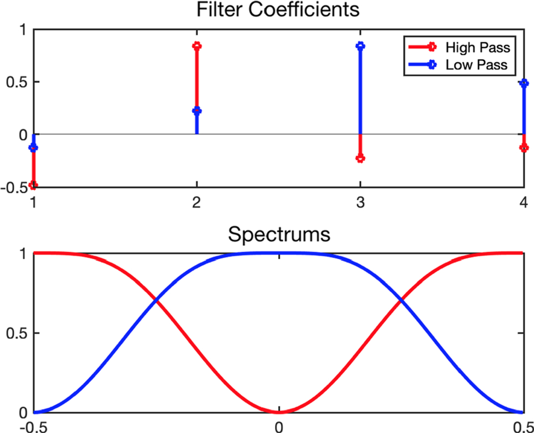
Discrete Daubechies-4 Wavelet Transform. (Top) The coefficients of the FIR filters. (Bottom) The spectrum of the same filters (sinc interpolated to 512 elements).

Fig. 2.

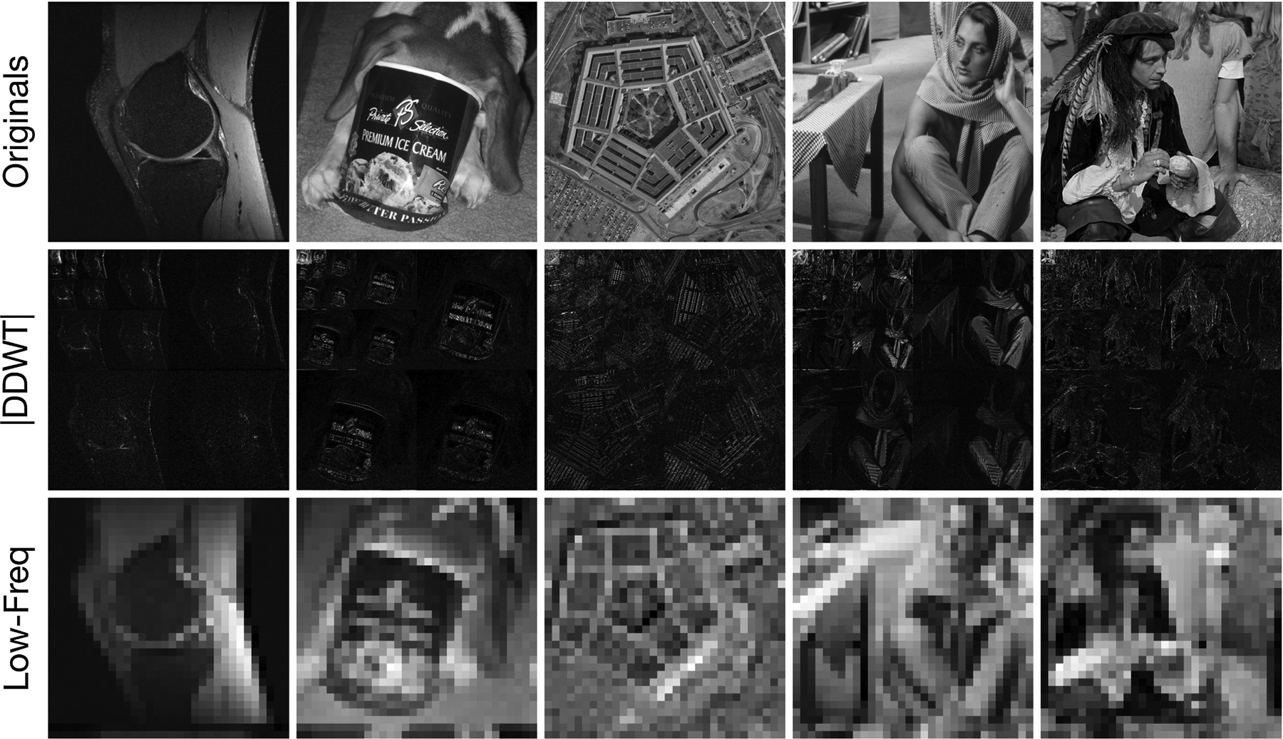
Wavelet Transforms of several different images. (Top) the original images, (Center) The magnitude of the Daubechies-4 wavelet transforms, (Bottom) the lowest-frequency bin of the wavelet transforms. Notably, the low frequency bin of the transform is not sparse (almost all values are non-zero).

Since the composition of FIR low-pass filters is an FIR low-pass filter, the lowest frequency bin in the transform domain is a low-pass filtered (and downsampled) image. The DDWT low-pass filters are not ideal filters (meaning that they have a non-zero transition region and that their support extends beyond the cutoff frequency); therefore, the lowest frequency bin of the transform also includes aliasing. Since the other bins of the Wavelet transform of natural images are sparse, by the sifting property of convolution, the aliasing artifacts present in the lowest frequency bin must also be sparse.

To estimate the lowest frequency bin, since it is not typically sparse for natural images, there is no advantage to utilizing the theory of compressed sensing. Instead, we can rely on the Nyquist-Shannon sampling theorem [12] and collect evenly spaced samples at twice the cutoff frequency. This technique, fully sampling a region centered on the 0 frequency in the Fourier domain, was developed as a heuristic and has been used extensively in compressed sensing [50, 51, 44, 32]. The size and shape of the fully sampled region, though, had not been theoretically justified in these techniques. For example, the SAKE method synthesizes a fully sampled square region of size 80 × 80 to reconstruct an image of size 200 × 200 [48]. The DISCO method uses a fully sampled spherical region [44, 32]. By only collecting the number of samples required to satisfy the Nyquist-Shannon theorem, the total number of samples is reduced over these heuristic techniques.

Let r denote the number of recursion levels of the DDWT. Then the size of the lowest frequency bin, after downsampling, would be (M/2^r)×(N/2^r) pixels², where the image is size M × N. Thus, its resolution would be (2^r/M) × (2^r/N). According to the Nyquist-Shannon theorem, this image can be reconstructed accurately if a rectangular region of size (2^r/M)×(2^r/N) with evenly spaced samples centered on the 0 frequency is collected; we denote this subset of samples as the Fully Sampled Region (FSR).

3. Methods

Our approach will be to first reconstruct a low-frequency image and then correct this estimate with high frequency information. One could reconstruct a low frequency image simply by performing an Inverse DFT on the data collected in the FSR. However, doing so leads to ringing (Gibbs phenomenon), which increases the energy in the high frequency bins of the wavelet transform of the image. Instead, we apply a separable Kaiser-Bessel window [28, 40] with a parameter of 4.

Let ${\widehat{y}}_L=F^{*}{K}_B{M}_{L}b$, where F* is the adjoint of the unitary F, and M_L and K_B are diagonal matrices representing the mask of the fully sampled region and the Kaiser-Bessel kernel, respectively. Then we wish to estimate y by solving the following problem:

$$\underset{y\in {ℂ}^N}{\text{minimize}}{\Vert W\left(y-{\widehat{y}}_L\right)\Vert }_1\text{\hspace{0.17em}subject\hspace{0.17em}to}\left(1/2\right){\Vert MFy-b\Vert }_2^2<ϵ.$$ (2)

The key insight is that $z=W\left(y-{\widehat{y}}_L\right)$ will be more sparse (have more values approximately equal to 0) than x for the reasons presented in section 2. Figure 3 shows z for the images of Fig. 2. Indeed, they are now better approximated by a sparse representation. With this definition of z, (2) is equivalent to

$$\underset{z\in {ℂ}^N}{\text{minimize}}{\Vert z\Vert }_1\text{\hspace{0.17em}subject\hspace{0.17em}to}\left(1/2\right){\Vert Az-\beta \Vert }_2^2<ϵ,$$ (3)

where $\beta =b-MF{\widehat{y}}_L$. After solving (3) for z^★, the image can be reconstructed with $y^{\star }=W^{-1}{z}^{\star }+{\widehat{y}}_L$. We call this the More Sparse Basis Pursuit Denoising (MSBPD) solution. Problem (3) is also a basis pursuit denoising problem; the difference between it and (1) is the data vector is replaced with β. Since A satisfies RIPL [33], the bound on the error provided in [7] applies. Since the vector z has more elements with value closer to 0, the error that results from solving (3) has a smaller bound than that of solving (1).

Fig. 3.

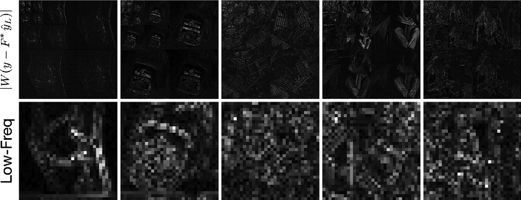
Wavelet transforms of images after subtracting the low-frequency reconstruction from the image. (Top) Wavelet transform with r = 4. (Bottom) lowest-frequency bin of the Wavelet transform. The lowest-frequency bin has many more values approximately equal to 0 than those of Fig. 2.

4. Results

All experiments in this study were performed with images of size 512 × 512. All optimization problems were solved using FISTA with line search [45, 9] run for 100 iterations. The wavelet transform applied was the DDWT-4, recursively applied to only the lowest-frequency bin r = 4 times. Figure 4 shows the sampling patterns used in the experiments with various sampling percentages with and without the fully sampled center region. The sampling patterns are realizations of a random separable Laplacian distribution [25] with a standard deviation of approximately 20%. This pattern has a higher probability of sampling higher frequencies than a Gaussian distribution with the same standard deviation. This likely better matches the actual power spectral density of natural images and is, therefore, a more optimal sampling pattern for a compressed sensing reconstruction [1]. For the sampling patterns with the fully sampled region, fewer samples from the distribution were included in order to retain approximately the same number of total samples. The value of was chosen independently for each reconstruction by conducting an exhaustive search to find the value that minimized the relative error $e={\Vert y^{\star }-y\Vert }_2/{\Vert y\Vert }_2$.

Fig. 4.

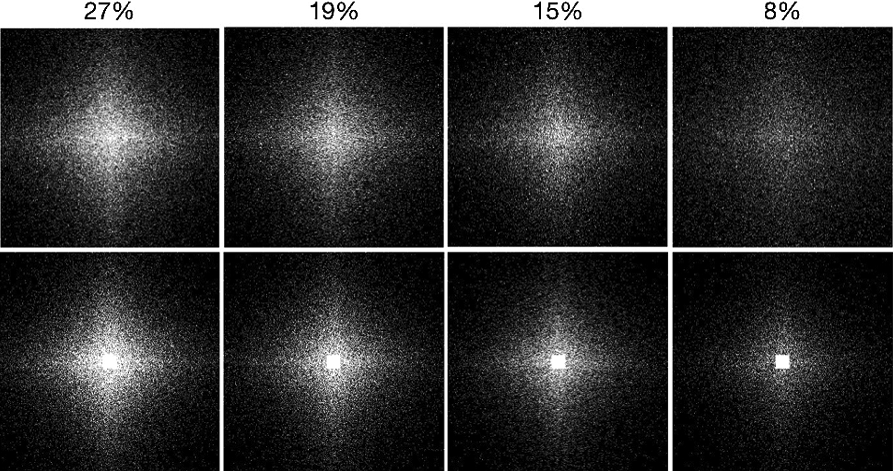
Variable density Fourier sampling patterns generated according to a separable Laplacian distribution. The top / bottom rows show the sampling patterns without / with the Fully sampled Region (FSR), respectively. The number of variable density samples is reduced when the FSR is included to maintain the sampling percentage.

Figure 5 shows reconstructions using BPD and MSBPD. As can be observed in Fig. 5, MSBPD offers the highest quality reconstruction for all sampling percentages. The improvements become more noticeable as the sampling percentage is reduced.

Fig. 5.

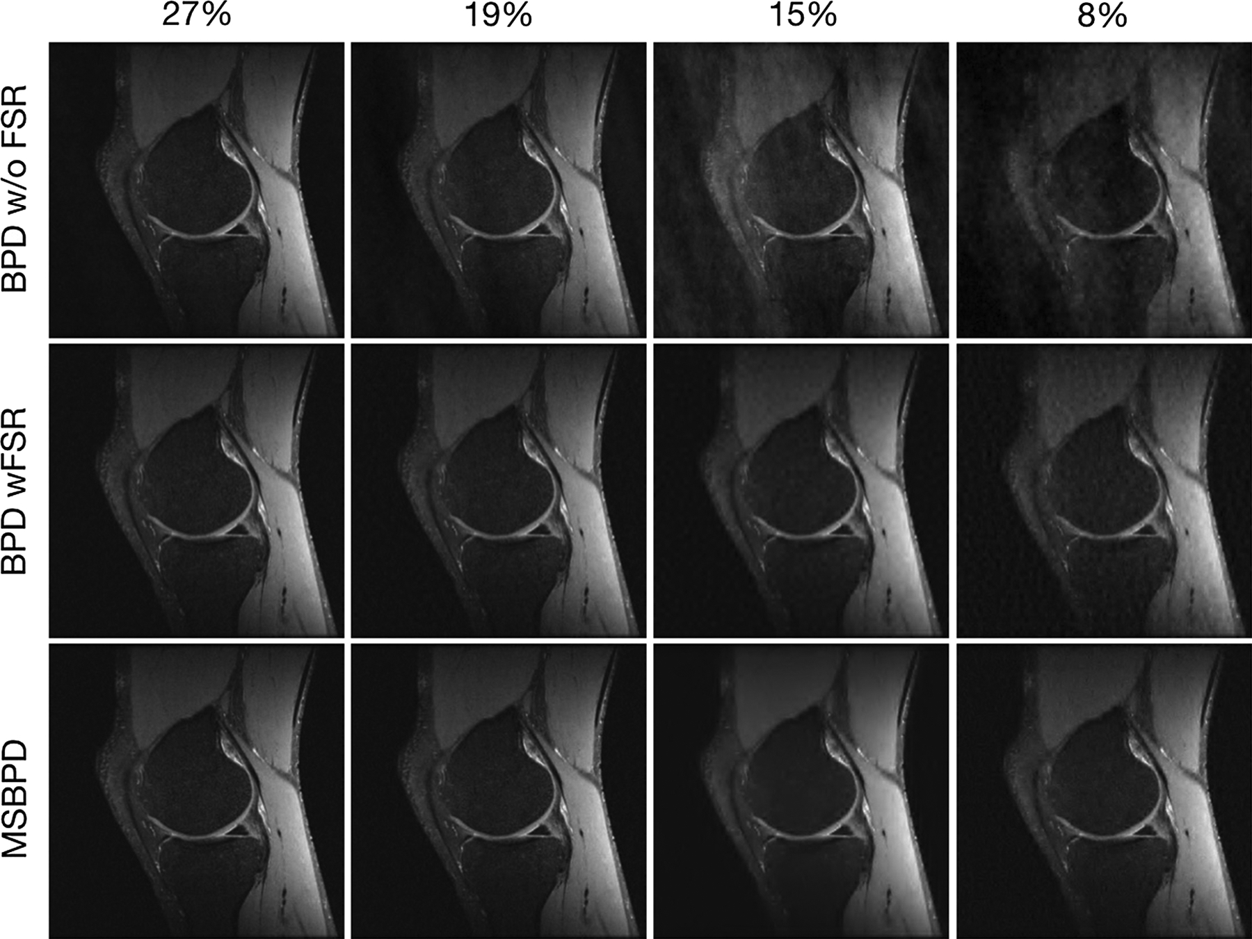
Reconstructions of MR images of the the knee with different sampling percentages without and with the Fully Sampled Region (FSR).

Table 1 shows the relative errors for the reconstructions in Fig. 5. In all cases, MSBPD yields the lowest relative error. The most significant improvement comes by including the FSR in the samples; a minor gain is attained by using MSBPD over BPD on this sampling pattern. The improvement is more pronounced as the sampling percentage decreases.

Table 1.

Relative errors for reconstructions of knee image from Fig. 2 with different sampling percentages.

Sampling Percentage	27%	19%	15%	8%
BPD	0.059	0.070	0.084	0.143
BPD w/FSR	0.058	0.068	0.076	0.113
MSBPD	0.056	0.065	0.071	0.093

Table 2 shows the Structural Similarity metric (SSIM) comparing the reconstructed images to the originals. This quantification shows the same trends as the relative errors.

Table 2.

SSIM values for reconstructions of knee image from Fig. 2 with different sampling percentages.

Sampling Percentage	27%	19%	15%	8%
BPD	0.996	0.995	0.992	0.977
BPD w/FSR	0.996	0.995	0.994	0.986
MSBPD	0.997	0.995	0.995	0.990

In Fig. 6, we zoom into the reconstruction of the knee from 8% of data. This figure shows fewer wavelet artifacts in the result of MSBPD than exist in the result of BPD with either sampling pattern.

Fig. 6.

Zoom in to reconstructions of MRI data of knee from 8% of the data. (a) shows the original image; (b) shows the reconstruction using BPD with variable density data; (c) shows the reconstruction using BPD with a fully sampled center region; and (d) shows reconstruction with MSBPD. The red arrows point to regions in the image where the improvement in quality of MSBPD over the other algorithms is very apparent.

Figure 7 shows the reconstructions with 8% of the data for BPD and MSBPD on all images of Fig. 2. Figure 8 shows the magnitudes of the differences between the reconstructions with 8% of the data shown in Fig. 7 and the original images. The errors are significantly reduced by including the FSR. There is an additional improvement to the reconstruction when using MSBPD.

Fig. 7.

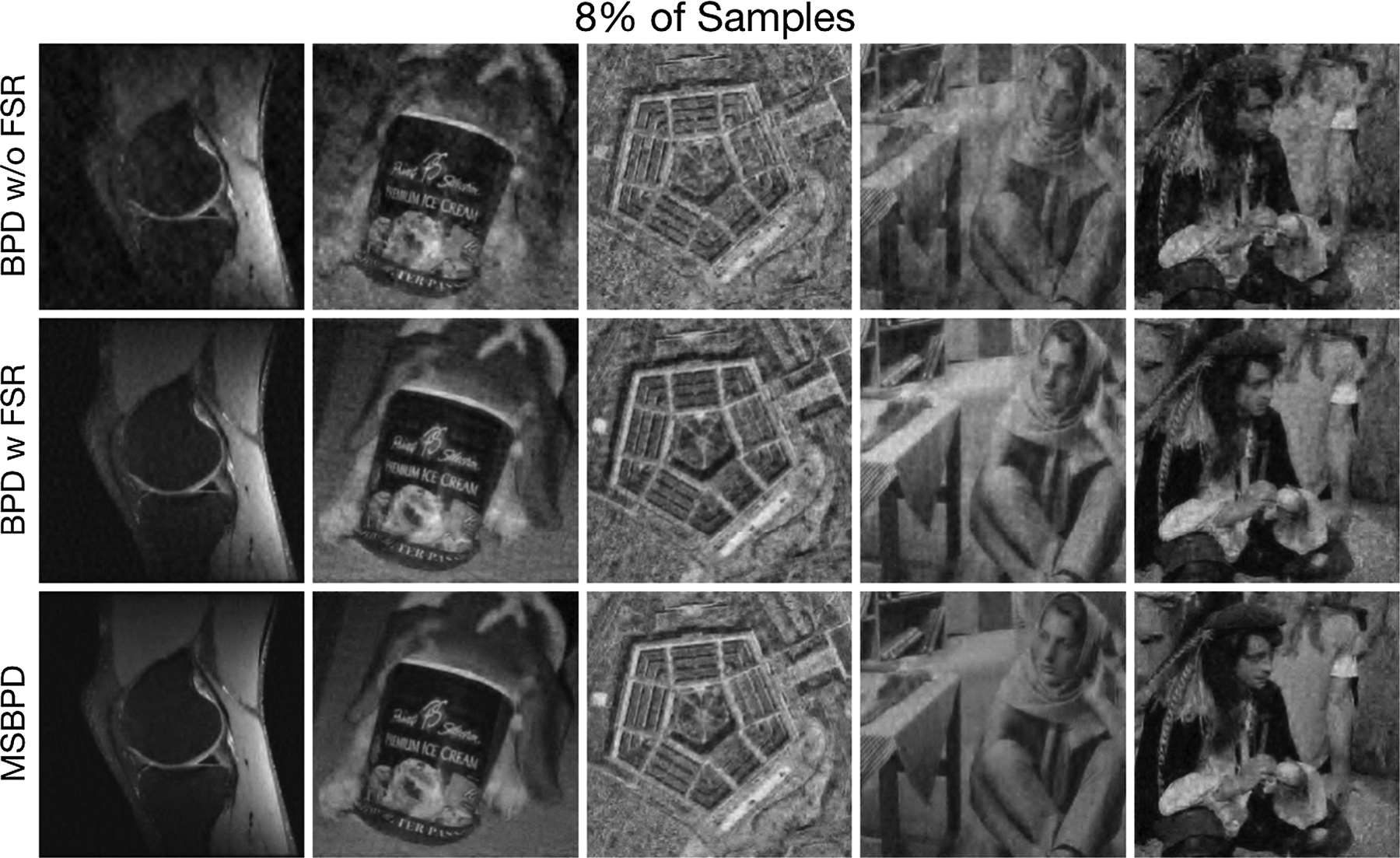
A comparison of BPD (without and with the FSR) to MSBPD with 8% of the sampling data for all images of Fig. 2. The quality of reconstruction with MSBPD is improved over the quality of BPD.

Fig. 8.

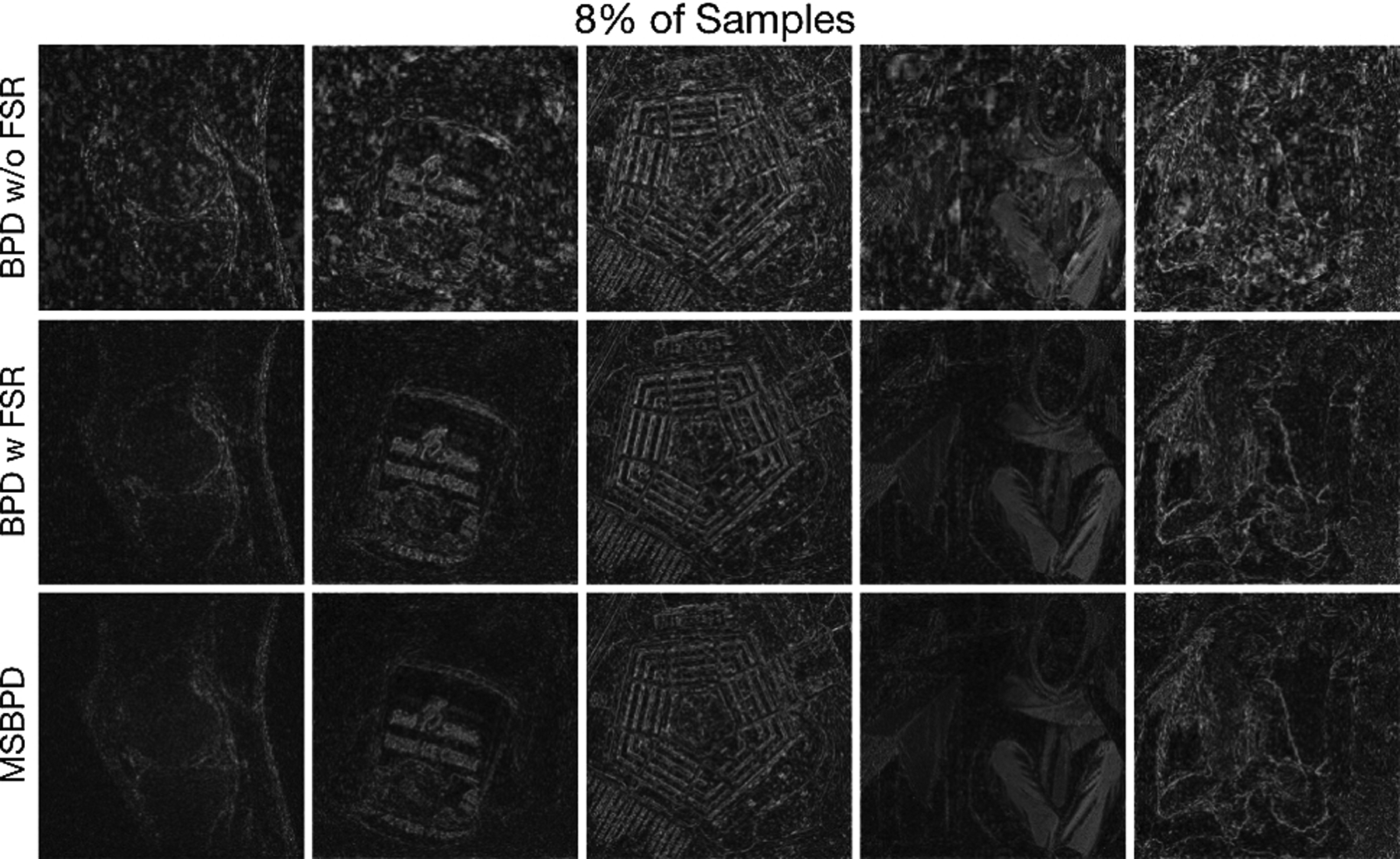
Magnitudes of the differences between the reconstructions of Fig. 7 and the original images shown in Fig. 2. There is a significant reduction in the error by including the FSR in the sampling pattern. An additional reduction in error is realized by using MSBPD.

Table 3 shows the relative error for each algorithm on each of the five reconstructions of Fig. 7. As observed previously, the most significant gain is attained by including the FSR. A minor additional gain is attained with MSBPD.

Table 3.

Relative error for reconstructions of all images from Fig. 2 with 8% of data.

Image Index	1	2	3	4	5
BPD	0.143	0.183	0.118	0.201	0.256
BPD w/FSR	0.093	0.131	0.104	0.147	0.169
MSBPD	0.093	0.113	0.103	0.143	0.159

Table 4 shows the Structural Similarity metric (SSIM) comparing the reconstructed images to the originals. Once again, this metric shows the same trends as the relative errors.

Table 4.

SSIM values for reconstructions of all images from Fig. 2 with 8% of data.

Image Index	1	2	3	4	5
BPD	0.977	0.921	0.699	0.866	0.878
BPD w/FSR	0.986	0.959	0.797	0.935	0.948
MSBPD	0.990	0.970	0.806	0.939	0.954

5. Discussion

In this work, we have utilized the structure of the Discrete Daubechies Wavelet Transform to improve image reconstruction results based on compressed sensing. It takes advantage of the prior knowledge that a great deal of images are not sparse in the lowest-frequency bin of the image’s wavelet transform.

Note that some images, those that are natively sparse, are indeed sparse in the lowest frequency bin of the DDWT; e.g. images of angiography and some astronomy. There would be no advantage to using MSBPD over BPD for images of that type, and other types of compressed sensing reconstruction algorithms may be more appropriate [21]. When it is the case, however, that the image is not sparse in the lowest frequency bin then MSBPD offers reconstruction with improved quality over BPD even when the sampling pattern includes the FSR.

Due to the increased sparsity, an accurate reconstruction may be possible using the greedy Orthogonal Matching Pursuit [41, 49] algorithm to solve the corresponding sparse signal recovery problem:

$$\underset{z\in {ℂ}^N}{\text{minimize}}(1/2)\Vert Az-\beta {\Vert }_2^2\text{subject\hspace{0.17em}to}{\Vert z\Vert }_0\le \mathcal{S},$$

where ∥·∥₀ is the L₀ penalty and $\mathcal{S}$ limits the number of non-zero elements in the vector z. This could make image reconstruction more computationally efficient.

The DDWT and the DFT are both radially asymmetric transforms; i.e., a rotation operator and the transform operator do not generally commute. However, in many imaging systems, there is not anything inherently special about the horizontal and vertical directions (e.g. MRI, CT, radio interferometry). Therefore, it may be possible to reconstruct images of higher quality by collecting a circle of data in the low-frequency region (rather than a square) and use a sparsifying transform that is radially symmetric. Symmetric wavelets on the sphere [31] may be such a sparsifying transform. Though this may yield improved quality, the computations required may increase. This side-effect of this possible improvement should be considered for any given application.

With each recursive application of the Wavelet transform, the average sparsity is reduced [2]. Thus, the value of r can be chosen based on the sparsity achievable for the imaging system and subjects of interest. Additionally, the higher the value of r, the more computations are required to implement the wavelet transform. Both aspects should be considered when determining a value of r for a given application.

In this work, we determined the regularization parameter with an exhaustive search. This is only appropriate when ground truth is known and not a practical solution. For some applications, the bound on the noise can be determined with an image of noise; this can be accomplished in MRI, for example, by imaging with an excitation of 0. When a calibration image is unavailable, reconstruction may be accomplished by adapting the MSBPD algorithm to an iterative re-weighting algorithm [15, 16, 4, 52]. Alternatively, an automatic parameter tuning algorithm can be used based on existing training data [30] or with properties of the resulting pareto-optimal set [47]. Some of these methods have the consequence of implicitly altering the objective function [15], which means that the theorems of compressed sensing no longer hold. However, they have been shown heuristically to improve image quality in some cases.

Finally, the method presented in this work can be adapted to situations where information is shared amongst several acquisitions. This can happen with multiple-acquisition MRI [46], parallel MRI [38], or synthetic-aperture radar imaging [58] and may involve joint-sparsity regularization [29]. Moreover, the method can be adapted to deep-learning methods that are regularized with wavelet sparsity or joint sparsity [23].

We leave the investigations of these possible extensions as future work.

6. Conclusion

In this work, we have presented the MSBPD algorithm. This algorithm utilizes the structure and behavior of the DDWT to justify a sampling pattern and to identify a new sparsifying transform that increases sparsity of most natural images. Since the system matrix satisfies RIPL, this leads to improved results over solving the standard BPD problem of (1). In experiments, we compared image quality of reconstructions made with BPD, BPD with the FSR, and MSBPD. In all cases, the most significant gain was attained by including the FSR in the sampling pattern and MSBPD yielded the lowest relative error.

References

- 1.Adcock B, Hansen A, Roman B: The quest for optimal sampling: Computationally efficient, structure-exploiting measurements for compressed sensing. math. FA 1403 (2014) [Google Scholar]
- 2.Adcock B, Hansen AC, Poon C, Roman B: Breaking the coherence barrier: A new theory for compressed sensing. In: Forum of Mathematics, Sigma, vol. 5. Cambridge University Press; (2017) [Google Scholar]
- 3.Antun V, Renna F, Poon C, Adcock B, Hansen AC: On instabilities of deep learning in image reconstruction-does AI come at a cost? arXiv preprint arXiv:1902.05300 (2019) [DOI] [PMC free article] [PubMed] [Google Scholar]
- 4.Asif MS, Romberg J: Fast and accurate algorithms for re-weighted ℓ1-norm minimization. IEEE Transactions on Signal Processing 61(23), 5905–5916 (2013) [Google Scholar]
- 5.Baron CA, Dwork N, Pauly JM, Nishimura DG: Rapid compressed sensing reconstruction of 3d non-cartesian MRI. Magnetic resonance in medicine 79(5), 2685–2692 (2018) [DOI] [PMC free article] [PubMed] [Google Scholar]
- 6.Bastounis A, Adcock B, Hansen A: From global to local: Getting more from compressed sensing. SIAM News (2017) [Google Scholar]
- 7.Bastounis A, Hansen AC: On the absence of the RIP in real-world applications of compressed sensing and the RIP in levels. arXiv preprint arXiv:1411.4449 (2014) [Google Scholar]
- 8.Bastounis A, Hansen AC: On the absence of uniform recovery in many real-world applications of compressed sensing and the restricted isometry property and nullspace property in levels. SIAM Journal on Imaging Sciences 10(1), 335–371 (2017) [Google Scholar]
- 9.Beck A, Teboulle M: A fast iterative shrinkage-thresholding algorithm for linear inverse problems. SIAM journal on imaging sciences 2(1), 183–202 (2009) [Google Scholar]
- 10.Becker S, Bobin J, Candès EJ: NESTA: A fast and accurate first-order method for sparse recovery. SIAM Journal on Imaging Sciences 4(1), 1–39 (2011) [Google Scholar]
- 11.Blunck Y, Kolbe SC, Moffat BA, Ordidge RJ, Cleary JO, Johnston LA: Compressed sensing effects on quantitative analysis of undersampled human brain sodium MRI. Magnetic Resonance in Medicine 83(3), 1025–1033 (2020) [DOI] [PubMed] [Google Scholar]
- 12.Bracewell RN: Two-dimensional imaging. Prentice-Hall, Inc. (1995) [Google Scholar]
- 13.Candès EJ, Romberg J, Tao T: Robust uncertainty principles: Exact signal reconstruction from highly incomplete frequency information. IEEE Transactions on information theory 52(2), 489–509 (2006) [Google Scholar]
- 14.Candès EJ, Wakin MB: An introduction to compressive sampling [a sensing/sampling paradigm that goes against the common knowledge in data acquisition]. IEEE signal processing magazine 25(2), 21–30 (2008) [Google Scholar]
- 15.Candès EJ, Wakin MB, Boyd SP: Enhancing sparsity by reweighted ℓ1 minimization. Journal of Fourier analysis and applications 14(5–6), 877–905 (2008) [Google Scholar]
- 16.Chartrand R, Yin W: Iteratively reweighted algorithms for compressive sensing. In: IEEE International Conference on Acoustics, Speech and Signal Processing, pp. 3869–3872. IEEE; (2008) [Google Scholar]
- 17.Chen S, Donoho D: Basis pursuit. In: Proceedings of 1994 28th Asilomar Conference on Signals, Systems and Computers, vol. 1, pp. 41–44. IEEE; (1994) [Google Scholar]
- 18.Chen SS, Donoho DL, Saunders MA: Atomic decomposition by basis pursuit. SIAM review 43(1), 129–159 (2001) [Google Scholar]
- 19.Cheng JY, Zhang T, Ruangwattanapaisarn N, Alley MT, Uecker M, Pauly JM, Lustig M, Vasanawala SS: Free-breathing pediatric MRI with nonrigid motion correction and acceleration. Journal of Magnetic Resonance Imaging 42(2), 407–420 (2015) [DOI] [PMC free article] [PubMed] [Google Scholar]
- 20.Choi K, Wang J, Zhu L, Suh TS, Boyd S, Xing L: Compressed sensing based cone-beam computed tomography reconstruction with a first-order method a. Medical physics 37(9), 5113–5125 (2010) [DOI] [PMC free article] [PubMed] [Google Scholar]
- 21.Cukur T, Lustig M, Saritas EU, Nishimura DG: Signal compensation and compressed sensing for magnetization-prepared MR angiography. IEEE transactions on medical imaging 30(5), 1017–1027 (2011) [DOI] [PMC free article] [PubMed] [Google Scholar]
- 22.Dai G, He Z, Sun H: Ultrasonic block compressed sensing imaging reconstruction algorithm based on wavelet sparse representation. Current Medical Imaging 16(3), 262–272 (2020) [DOI] [PubMed] [Google Scholar]
- 23.Dar SU, Yurt M, Shahdloo M, Ildız ME, Tınaz B, Çukur T: Prior-guided image reconstruction for accelerated multi-contrast MRI via generative adversarial networks. IEEE Journal of Selected Topics in Signal Processing 14(6), 1072–1087 (2020) [Google Scholar]
- 24.Datta S, Deka B: Group-sparsity based compressed sensing reconstruction for fast parallel MRI. In: International Conference on Pattern Recognition and Machine Intelligence, pp. 70–77. Springer; (2019) [Google Scholar]
- 25.Fang Z, Van Le N, Choy M, Lee JH: High spatial resolution compressed sensing (HSPARSE) functional MRI. Magnetic resonance in medicine 76(2), 440–455 (2016) [DOI] [PMC free article] [PubMed] [Google Scholar]
- 26.Folberth J, Becker S: Efficient adjoint computation for wavelet and convolution operators. IEEE Signal Processing Magazine 33(6), 135–147 (2016) [Google Scholar]
- 27.Huang YC, Chang SC: Error resilient techniques for wavelet based compressed sensing. In: 2020 IEEE 2nd Global Conference on Life Sciences and Technologies (LifeTech), pp. 39–41. IEEE; (2020) [Google Scholar]
- 28.Kaiser JF: Nonrecursive digital filter design using the i_0-sinh window function. In: Proc. 1974 IEEE International Symposium on Circuits & Systems, San Francisco DA, April, pp. 20–23 (1974) [Google Scholar]
- 29.Kopanoglu E, Güngör A, Kilic T, Saritas EU, Oguz KK, Çukur T, Güven HE: Simultaneous use of individual and joint regularization terms in compressive sensing: Joint reconstruction of multi-channel multi-contrast MRI acquisitions. NMR in Biomedicine 33(4), e4247 (2020) [DOI] [PubMed] [Google Scholar]
- 30.Kunisch K, Pock T: A bilevel optimization approach for parameter learning in variational models. SIAM Journal on Imaging Sciences 6(2), 938–983 (2013) [Google Scholar]
- 31.Lessig C, Fiume E: SOHO: Orthogonal and symmetric haar wavelets on the sphere. ACM Transactions on Graphics (TOG) 27(1), 4 (2008) [Google Scholar]
- 32.Levine E, Daniel B, Vasanawala S, Hargreaves B, Saranathan M: 3D cartesian MRI with compressed sensing and variable view sharing using complementary poisson-disc sampling. Magnetic resonance in medicine 77(5), 1774–1785 (2017) [DOI] [PMC free article] [PubMed] [Google Scholar]
- 33.Li C, Adcock B: Compressed sensing with local structure: uniform recovery guarantees for the sparsity in levels class. Applied and Computational Harmonic Analysis 46(3), 453–477 (2019) [Google Scholar]
- 34.Li F, Cornwell TJ, de Hoog F: The application of compressive sampling to radio astronomy - i. deconvolution. Astronomy & Astrophysics 528, A31 (2011) [Google Scholar]
- 35.Lustig M, Donoho D, Pauly JM: Sparse MRI: The application of compressed sensing for rapid MR imaging. Magnetic Resonance in Medicine: An Official Journal of the International Society for Magnetic Resonance in Medicine 58(6), 1182–1195 (2007) [DOI] [PubMed] [Google Scholar]
- 36.Maier A, Syben C, Lasser T, Riess C: A gentle introduction to deep learning in medical image processing. Zeitschrift für Medizinische Physik 29(2), 86–101 (2019) [DOI] [PubMed] [Google Scholar]
- 37.Majumdar A, Ward RK: On the choice of compressed sensing priors and sparsifying transforms for MR image reconstruction: An experimental study. Signal Processing: Image Communication 27(9), 1035–1048 (2012) [Google Scholar]
- 38.Murphy M, Alley M, Demmel J, Keutzer K, Vasanawala S, Lustig M: Fast ℓ1-spirit compressed sensing parallel imaging MRI: Scalable parallel implementation and clinically feasible runtime. IEEE transactions on medical imaging 31(6), 1250–1262 (2012) [DOI] [PMC free article] [PubMed] [Google Scholar]
- 39.Oike Y, El Gamal A: CMOS image sensor with percolumn σδ ADC and programmable compressed sensing. IEEE Journal of Solid-State Circuits 48(1), 318–328 (2012) [Google Scholar]
- 40.Oppenheim AV, Schafer RW: Discrete-time signal processing. Pearson Education; (2014) [Google Scholar]
- 41.Pati YC, Rezaiifar R, Krishnaprasad PS: Orthogonal matching pursuit: Recursive function approximation with applications to wavelet decomposition. In: Proceedings of 27th Asilomar conference on signals, systems and computers, pp. 40–44. IEEE; (1993) [Google Scholar]
- 42.Poon C: On the role of total variation in compressed sensing. SIAM Journal on Imaging Sciences 8(1), 682–720 (2015) [Google Scholar]
- 43.Sandino CM, Cheng JY, Chen F, Mardani M, Pauly JM, Vasanawala SS: Compressed sensing: From research to clinical practice with deep neural networks: Shortening scan times for magnetic resonance imaging. IEEE Signal Processing Magazine 37(1), 117–127 (2020) [DOI] [PMC free article] [PubMed] [Google Scholar]
- 44.Saranathan M, Rettmann DW, Hargreaves BA, Clarke SE, Vasanawala SS: Differential subsampling with cartesian ordering (DISCO): A high spatio-temporal resolution dixon imaging sequence for multiphasic contrast enhanced abdominal imaging. Journal of Magnetic Resonance Imaging 35(6), 1484–1492 (2012) [DOI] [PMC free article] [PubMed] [Google Scholar]
- 45.Scheinberg K, Goldfarb D, Bai X: Fast first-order methods for composite convex optimization with backtracking. Foundations of Computational Mathematics 14(3), 389–417 (2014) [Google Scholar]
- 46.Senel LK, Kilic T, Gungor A, Kopanoglu E, Guven HE, Saritas EU, Koc A, Cukur T: Statistically segregated k-space sampling for accelerating multiple-acquisition MRI. IEEE transactions on medical imaging 38(7), 1701–1714 (2019) [DOI] [PubMed] [Google Scholar]
- 47.Shahdloo M, Ilicak E, Tofighi M, Saritas EU, Çetin AE, Çukur T: Projection onto epigraph sets for rapid self-tuning compressed sensing MRI. IEEE transactions on medical imaging 38(7), 1677–1689 (2018) [DOI] [PubMed] [Google Scholar]
- 48.Shin PJ, Larson PE, Ohliger MA, Elad M, Pauly JM, Vigneron DB, Lustig M: Calibrationless parallel imaging reconstruction based on structured low-rank matrix completion. Magnetic resonance in medicine 72(4), 959–970 (2014) [DOI] [PMC free article] [PubMed] [Google Scholar]
- 49.Tropp JA, Gilbert AC: Signal recovery from random measurements via orthogonal matching pursuit. IEEE Transactions on information theory 53(12), 4655–4666 (2007) [Google Scholar]
- 50.Uecker M, Lai P, Murphy MJ, Virtue P, Elad M, Pauly JM, Vasanawala SS, Lustig M: ESPIRiT—an eigenvalue approach to autocalibrating parallel mri: where SENSE meets GRAPPA. Magnetic resonance in medicine 71(3), 990–1001 (2014) [DOI] [PMC free article] [PubMed] [Google Scholar]
- 51.Vasanawala S, Murphy M, Alley MT, Lai P, Keutzer K, Pauly JM, Lustig M: Practical parallel imaging compressed sensing MRI: Summary of two years of experience in accelerating body MRI of pediatric patients. In: 2011 IEEE international symposium on biomedical imaging: From nano to macro, pp. 1039–1043. IEEE; (2011) [DOI] [PMC free article] [PubMed] [Google Scholar]
- 52.Voronin S, Daubechies I: An iteratively reweighted least squares algorithm for sparse regularization. arXiv preprint arXiv:1511.08970 (2015) [Google Scholar]
- 53.Wiaux Y, Jacques L, Puy G, Scaife AM, Van-dergheynst P: Compressed sensing imaging techniques for radio interferometry. Monthly Notices of the Royal Astronomical Society 395(3), 1733–1742 (2009) [Google Scholar]
- 54.Xu X, Zhang M, Luo M, Yang J, Qu Q, Tan Z, Yang H: Echo signal extraction based on improved singular spectrum analysis and compressed sensing in wavelet domain. IEEE Access; 7, 67402–67412 (2019) [Google Scholar]
- 55.Zhang J, Ghanem B: ISTA-Net: Interpretable optimization-inspired deep network for image compressive sensing. In: Proceedings of the IEEE conference on computer vision and pattern recognition, pp. 1828–1837 (2018) [Google Scholar]
- 56.Zhang J, Teng J, Bai Y: Improving sparse compressed sensing medical CT image reconstruction. Automatic Control and Computer Sciences 53(3), 281–289 (2019) [Google Scholar]
- 57.Zhu B, Liu JZ, Cauley SF, Rosen BR, Rosen MS: Image reconstruction by domain-transform manifold learning. Nature 555(7697), 487–492 (2018) [DOI] [PubMed] [Google Scholar]
- 58.Zhu XX, Ge N, Shahzad M: Joint sparsity in SAR tomography for urban mapping. IEEE Journal of Selected Topics in Signal Processing 9(8), 1498–1509 (2015) [Google Scholar]