Renal Cortex, Medulla and Pelvicaliceal System Segmentation on Arterial Phase CT Images with Random Patch-based Networks

Abstract

Renal segmentation on contrast-enhanced computed tomography (CT) provides distinct spatial context and morphology. Current studies for renal segmentations are highly dependent on manual efforts, which are time-consuming and tedious. Hence, developing an automatic framework for the segmentation of renal cortex, medulla and pelvicalyceal system is an important quantitative assessment of renal morphometry. Recent innovations in deep methods have driven performance toward levels for which clinical translation is appealing. However, the segmentation of renal structures can be challenging due to the limited field-of-view (FOV) and variability among patients. In this paper, we propose a method to automatically label the renal cortex, the medulla and pelvicalyceal system. First, we retrieved 45 clinically-acquired deidentified arterial phase CT scans (45 patients, 90 kidneys) without diagnosis codes (ICD-9) involving kidney abnormalities. Second, an interpreter performed manual segmentation to pelvis, medulla and cortex slice-by-slice on all retrieved subjects under expert supervision. Finally, we proposed a patch-based deep neural networks to automatically segment renal structures. Compared to the automatic baseline algorithm (3D U-Net) and conventional hierarchical method (3D U-Net Hierarchy), our proposed method achieves improvement of 0.7968 to 0.6749 (3D U-Net), 0.7482 (3D U-Net Hierarchy) in terms of mean Dice scores across three classes (p-value < 0.001, paired t-tests between our method and 3D U-Net Hierarchy). In summary, the proposed algorithm provides a precise and efficient method for labeling renal structures.

1. INTRODUCTION

Imaging of renal structures using computed tomography (CT) aids in various clinical indications, including diagnosis, evaluation, and treatment delivery for renal abnormalities such as artery stenosis, renal fusion, and nephroblastoma [1, 2]. As shown in Figure 1, kidney substructures consist of 1) the renal cortex; 2) the medulla; and 3) the renal pelvicalyceal system. The cortex forms the outer kidney layer and is contiguous with renal columns that descend between the renal pyramids. Both contain glomeruli and tubules, which form the functioning units of the kidney, the nephrons [3]. The medulla is organized into multiple cone-shaped pyramids, which include collecting ducts that drain into the renal calyces. Minor renal calyces coalesce into major calyces, which drain into the renal pelvis that drains into the ureter and ultimately into the bladder for voiding of urine to the exterior [4]. Anatomical differences between individuals give rise to differences in numbers and positioning on renal pyramids, minor and major calyces, and differences in the size and divisions of the renal pelvises [5]. Herein, accurate evaluation of renal structures offers clinicians better understanding of the kidney morphology and therefore improves treatment procedures. Contrast-enhanced CT is used as an important means of providing imaging contrast and characterizing kidney function and physiology [6, 7]. For acquiring visible enhancement of renal structures, the arterial phase is selected, which is a short phase that is collected about 15–25 seconds after contrast medium injection as shown in Figure 2 [8].

Figure 1.

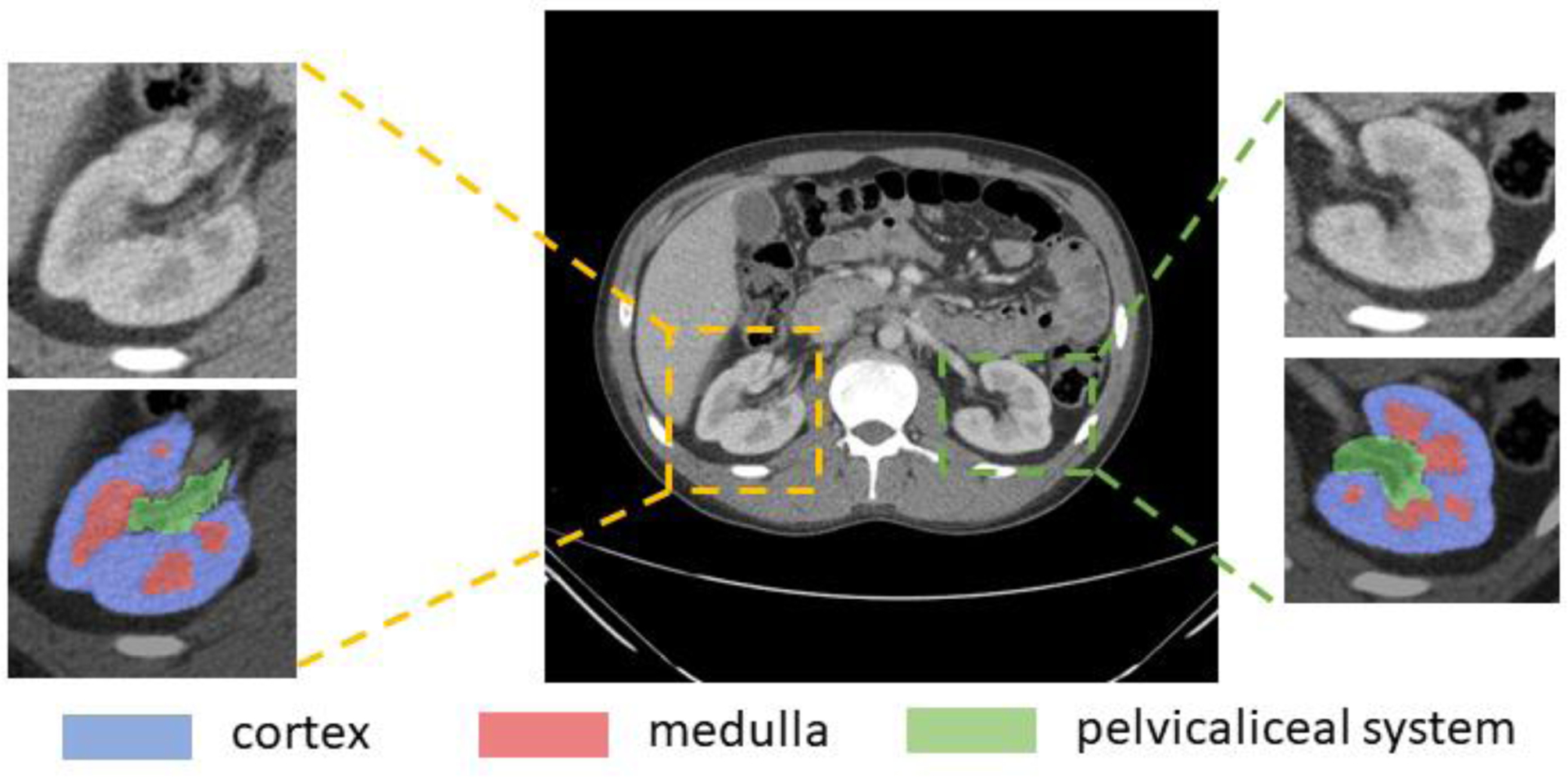
Renal structures segmentation of clinically acquired CT image. Yellow box shows a representative right kidney, green box shows the left kidney. The zoom-in patches show the CT kidney field-of-view (FOV) and labels. The label patches display the renal cortex (blue), the medulla (red) and the pelvicalyceal system (green). Those small structures make automatic renal segmentation challenging.

Figure 2.

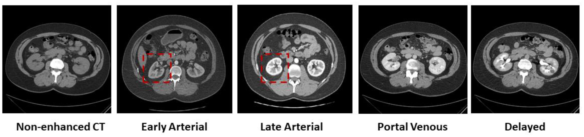
Five representative contrast enhancement phases in CT images, including non-enhanced CT, early arterial phase, late arterial phase, portal venous phase and delayed phase CT. Among these commonly used CT imaging phases, arterial scans (both early and late arterial phases) show clearer contrast of renal structures (the cortex, the medulla and the pelvicalyceal system) as shown in red boxes.

The considerable interest in and study of renal substructures are highly dependent on manual annotations, which is time consuming and tedious. In the past years, there have been pioneer investigations [9, 10] in renal cortex segmentation on MRI and CT images. Several algorithms have been designed to perform semi-automatic renal cortex segmentation [11, 12]. Many attempts at fully automatic segmentation have also spurred movement toward efficient cortex labeling of MRI images [13]. Historically, these studies provided compelling investigations on specific kidney donors but have not yet looked at multiple renal substructures in healthy kidneys. In recent studies, several kidney segmentation methods have been proposed and have achieved promising performance boosted by deep neural networks [14–17]. 3D methods were also explored for medical image segmentations [18–20]. However, most automatic algorithms focused on whole kidneys (right and left) or single tissue type (i.e. cortex segmentation) [8, 10, 21].

In this paper, we explore an automatic algorithm to segment three renal structures including the cortex, the medulla and the pelvicaliceal system. We propose a coarse-to-fine framework based on deep neural networks, a regime of increasing resolution at successive stages called random patch network fusion (RPFN). This technique includes a kidney detector and a patch-wise segmentor. In RPFN, we utilized both advantages of the full context in entire CT volumes (low resolution) and smoother boundary in patch-wise volumes (high resolution). We performed multiple random sampled patches and fuse the second segmentation model with the low resolution contexts.

We retrieved 45 deidentified CT images under IRB approval, and manually assessed ICD-9 codes for identifying normal kidneys in adults (age 18–50 years). Then, a trained interpreter manually traced right and left renal structures on these subjects under expert supervision. To evaluate our method, we compared methods of 3D U-Net [14] and hierarchical architectures [22] for 3D medical image segmentation. To the best of our knowledge, this is the first work that investigates an automatic method for renal multi-structure segmentation.

In summary, our contribution in this study are as follows:

• We retrieved 45 arterial CT scans and performed electronic health record data-based filtering mainly focused on demographics and ICD-9 codes.

• We manually labeled 45 subjects, with structures from 90 kidneys, including the renal cortex, the medulla and the pelvicalyceal system.

• We proposed a coarse-to-fine method called random patch network fusion, which learns renal segmentation both in low resolution and high resolution perspective.

• We evaluated the performance of the proposed algorithm as compared to the baseline that defines the state-of-the-art performance on multi-structure renal segmentation.

2. METHOD

We present an algorithm for renal segmentation on clinically acquired arterial phase CT scans. Images from 45 patients were manually labelled and introduced into the training dataset under the RPFN architecture and evaluated under a “leave-out” testing cohort, as seen in Figure 3. The RPFN is motivated by the coarse-to-fine framework and random patch-based methods, and employed to adapt renal segmentation tasks.

Figure 3.

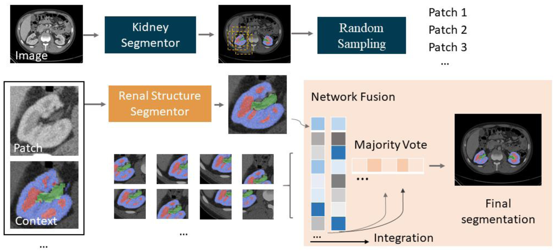
Method framework. The top pipeline shows the low resolution model, which aims to detect location of kidneys. After acquiring the coarse segmentation mask, random sampling is performed and cropped to presented CT and context patches. The bottom pipeline shows the patch-based renal structures segmentor followed by the network fusion step.

2.1. CT Imaging

Abdominal images were acquired from scans performed at Vanderbilt University Medical Center (VUMC). We performed de-identified data retrieval from the ImageVU project. This retrospective study was approved by the Institutional Review Board (IRB). Initially, data from 2000 patients were retrieved. In order to obtain comprehensive evaluation, we used exclusion criteria for identifying normal kidneys from the cohort. Out of 2000, 720 potential subjects were selected after assessment by excluding 992 ICD-9 codes related to kidney dysfunction and including age 18–50. For example, subjects with ICD-9 CM code 585.9 group (kidney disease) were excluded. Filtering and exclusion criteria were supervised by kidney disease experts and radiologists. A subset of subjects was categorized by ICD-10 codes; these ICD-10 codes were converted to ICD-9 standard. Out of 720 potential subjects, we limited our study to those who had arterial abdominal CT scans, which yielded 101 subjects. Among the 101 patients, we selected 23 female subjects and 22 male subjects, with a median age of 35.

All CT examinations were performed with Philips or Siemens CT scanners. Before image acquisition, patients were injected with 120–140 ml of contrast agent. CT scans were acquired at 25–35 seconds during imaging cycles. The in-plane pixel dimension ranged from 0.78–0.86 mm. Slice thickness ranged from 1.2–3.5 mm. The number of slices ranged from 80–120. Electronic health records (EHR), including demographics, ICD codes were retrieved for all subjects.

2.2. Manual Segmentation

With the 45 arterial CT scans from ImageVU, we manually annotated the renal cortex, the medulla and pelvicalyceal system for both right and left kidneys. A window level of −30 and 200 Hounsfield units (HU) was used, respectively. One trained interpreter performed manual labeling for each patient under expert supervision. Annotations were made on the axial slices of the scans while also consulting the sagittal and coronal views. The medulla and the pelvicaliceal system in many scans are very small structures, displaying a weak boundary between them. The pelvicaliceal system is the initial section of the ureter, connected from numerous ducts. The calyces and pelvis are included in the kidney as the main contours of the pelvicalyceal system, and the ureter was excluded. These tracing guidelines were followed consistently for all slices. The interpreters are supervised by experienced radiologists (> 10 years of experience in kidney radiology). When labeling cortex and medulla, the manual labels were checked against each other to ensure no overlap between the manual segmentations of the two anatomies. We manually traced the contour of the cortex and medulla boundaries to define the outer zone and inner layer slice by slice. The outer cortical tissues and renal columns are classified as the cortex label, the inner cone-shaped lobes are identified as the medulla.

2.3. Automatic Segmentation: Random Patch Network Fusion

As shown in Figure 3, the proposed algorithm for renal segmentation consists of two sections: 1) a 3D kidney detector that produce coarse segmentations, and 2) a renal structures segmentor which trained on imposed field of view (FOV) constraints. The final segmentation is formed by statistical fusion. Between two sections, the imposed FOV is sampled randomly.

1). Kidney Detector:

Using the manually labeled image as the ground truth. Consider the segmentor network parameterized by θ. The model aims to:

$$\underset{{\theta }_l,Y_l}{\text{argmin}}{L}_{D_l}\left({\theta }_l\right)$$ (1)

where $L_{D_l}\left({\theta }_l\right)$ is the Multi-Sourced Dice Loss (MSDL) [23]. MSDL was proposed as a way of evaluating datasets with multiple labels with a score by extending the Dice loss to adapt renal segmentation,

$$L_{D_l}=-\frac{2}{A}\frac{{\sum }_{a=0}^{A}w{\sum }_{i=1}^M{\sum }_{j=1}^N{Y}_{ij}{P}_{ij}+ϵ}{{\sum }_{a=0}^{A}w{\sum }_{i=1}^M{\sum }_{j=1}^N{Y}_{ij}^2+{\sum }_{a=0}^{A}w{\sum }_{i=1}^M{\sum }_{j=1}^N{P}_{ij}^2+ϵ}$$ (2)

where A denotes the number of anatomies and w represents the variance to different label set properties in given image dimension of M and N. Y is the voxel value and P are the predicted probability maps. A small number, ∈, was used in computing the prediction and voxel value correlation to prevent discontinuities. MSDL was iteratively optimized, and P_ij was computed by the softmax of the probability of voxel j in image i to anatomy a.

After acquiring the coarse segmentation masks, we randomly picked predicted pixels in the coarse segmentation. Using the selected pixel as indices’ center, we used a bounding box as the local FOV. In order to perform randomness, a random shift was added. The distance of shifting was derived by a random number generator with mean and variance among bounding boxes centers.

2). Renal Structure Segmentor:

In the second segmentation model, we built the hierarchy of non-linear features from random patches regardless of the anatomical context. It utilized detailed smoothness at original resolution and incorporated advantages of data augmentation with random shifting. Random patches have overlapped regions that provide multiple labels for single voxel. Herein, each voxel label was given by a vector of class values from n candidates. In RPFN, the majority vote was used as the label fusion algorithm, which fused n candidates from predictions to a single voxel. The final mask for voxel j in image i was acquired by:

$$S_{ij}=\mathit{\text{argmax}}\frac{1}{n}\sum _{m=1}^{n}p\left(a\mid s^{\prime },j\right)$$ (3)

where p(a|s′, j) = 1 if s′equals to anatomy class a and 0 otherwise. Voters outside the image space are ignored, whose related values are excluded in the label fusion.

2.4. Preprocessing

The manual annotations and corresponding arterial CT images were preprocessed in three steps. First, original CT scans were clipped by soft tissue window with range of [−175, 250] HU. Second, soft-tissue windowed images and labels were normalized and re-sampled using spline interpolation. In the kidney detector, the input volume is processed to 168×168×64 with intensity range from 0 to 1.

2.5. Experiment Design

We implemented experiments with maximum number (50) of patches for evaluating performance of baselines and RPNF. We implemented experiments with 5 fold cross validation. To perform standard five-fold cross validation, we split 25 scans into five complementary folds, each of which contains 5 cases. For each fold evaluation, we use 20 folds as training and validation on the remaining 5 cases.

We compared RPNF with three baseline architectures (low-resolution and hierarchy) with the same dataset and parameters. Briefly, we first trained the low-resolution approach, which has shown its capability on 3D renal segmentation with full spatial contexts.

2.6. Implementation details

We adopted 3D U-Net [14] as the segmentation model backbone, which contains encoder and decoder paths with four levels resolution. It employs deconvolution to up-sample the lower level feature maps to the higher space of images. This process enables the efficient denser pixel-to-pixel mappings. Each level in the encoder consists two 3×3×3 convolutional layers, followed by rectified linear units (ReLU) and a max pooling of 2×2×2 and strides of 2. In the decoder, the transpose convolutions of 2×2×2 and strides of 2 are used. The last layer is a 1×1×1 convolution that set the number of output channels to the number of class labels. We used Multi-sourced Dice Loss and Dice Loss for multi-organ segmentation and single class segmentation, respectively. The baseline low-resolution segmentation uses the largest volume size of 168 × 168 × 64 in order to fit maximum memory of a normal 12GB GPU under architecture of 3D U-Net. The volume size is also employed in baseline hierarchical method for training the first level model. We used batch size of 1 for all implementations. We used instance normalization, which is agnostic to batch size. We adapted ADAM algorithm with SGD, momentum=0.9. The initial learning rate was set to 0.001, and it was reduced by a factor of 10 every 10 epochs after 50 epochs. Implementations were performed using NVIDIA Titan X GPU 12G memory and CUDA 9.0.

3. RESULTS

Figure 4 and Table 1 compares the Dice scores of the renal cortex, the medulla and the pelvicalyceal system between the baseline and our proposed algorithm. The box plots presented were evaluated across 20 external testing subjects. The Dice values shown in Figure 4 are average performances across 5-fold cross-validation. Figure 4 indicates our algorithm achieved significant improvement compared with performance of segmentation baselines. The Dice scores of the RPFN are significantly superior to the Hierarchy algorithm across all three renal structures marked with ‘*’ (paired t-test p-value < 0.001). The mean and variance DSC for the cortex are 0.7637 ± 0.0516 (3D U-Net), 0.8146 ± 0.0504 (3D U-Net Hierarchy) and 0.8475± 0.0487 (RPFN), the mean DSC and variance DSC for the medulla are 0.6639 ± 0.0467 (3D U-Net), 0.7349 ± 0.0452 (3D U-Net Hierarchy) and 0.7895± 0.0429 (RPFN), the mean and variance DSC for the pelvicalyceal system are 0.5972 ± 0.0482 (3D U-Net), 0.6951 ± 0.0471 (3D U-Net Hierarchy) and 0.7533± 0.0453 (RPFN), respectively. Overall, the RPFN achieves improvement of 0.7968 to 0.6749(3D U-Net), 0.7482 (3D U-Net Hierarchy) in terms of mean Dice scores across three classes (p-value < 0.001, paired t-test). Figure 5 compares the qualitative result of 3D U-Net, Hierarchy and our method. The 3D U-Net Hierarchy method and RPNF achieve smoother boundaries among the medullas and cortex. RPFN shows more detailed structures than the result from 3D U-Net Hierarchical approach. Figure 6 shows the training and validation loss values to show the sensitivity of our method. The curve was evaluated by averaging five-fold cross validation and the shadow shows the variance of these five folds experiments. The 3D U-Net Hierarchical approach increases training resolution in the second step and achieved higher DSC than low resolution 3D U-Net. However, the hierarchical method’s performance is limited due to inaccurate localization from previous segmentation.

Figure 4.

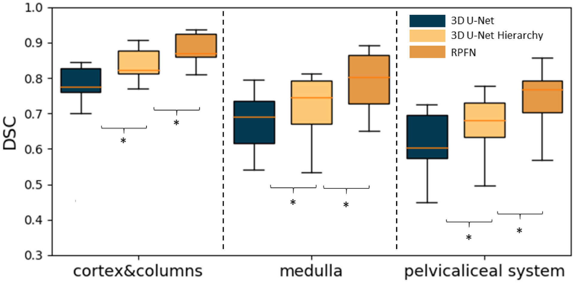
Boxplot of Dice similarity coefficient (DSC) on 20 external testing images. The result is the average across five-fold cross-validation. “*” indicates statistically significant differences (p<0.001 from paired t-test on mean DSC). We compared our method with two baseline approaches including 3D U-Net and 3D U-Net Hierarchy.

Table 1.

Summarized statistics for the final automatic system compared to manual segmentation

	Cortex	Medulla	Pelvicalyceal System
Hausdorff Distance	22.2424±19.9501	23.5101±14.1528	36.6512±12.1899
R Squared	0.8392	0.6319	0.3412
Pearson R	0.9681	0.7395	0.6029
Absolute deviation of volume (cm3)	5.5010±2.9511	4.6129±1.6511	1.3512±0.9158
Percent difference (%)	8.5159±3.5912	21.6193±10.6509	26.4501±19.9912

Figure 5.

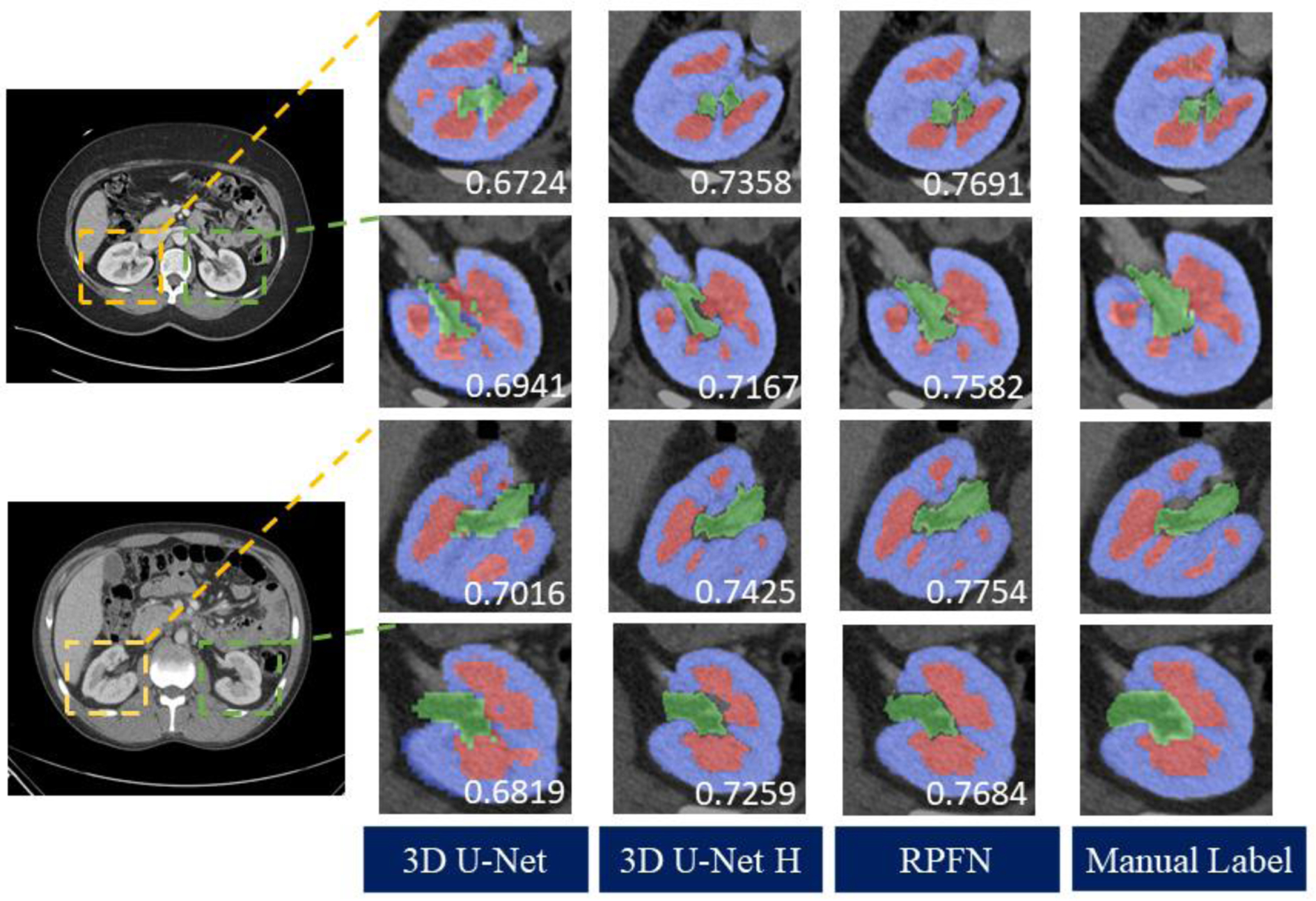
Qualitative result of two representative subjects. We compared the RPFN with two baseline methods as well as the ground truth. Yellow boxes show the right kidneys, green boxes display the left kidney structures.

Figure 6.

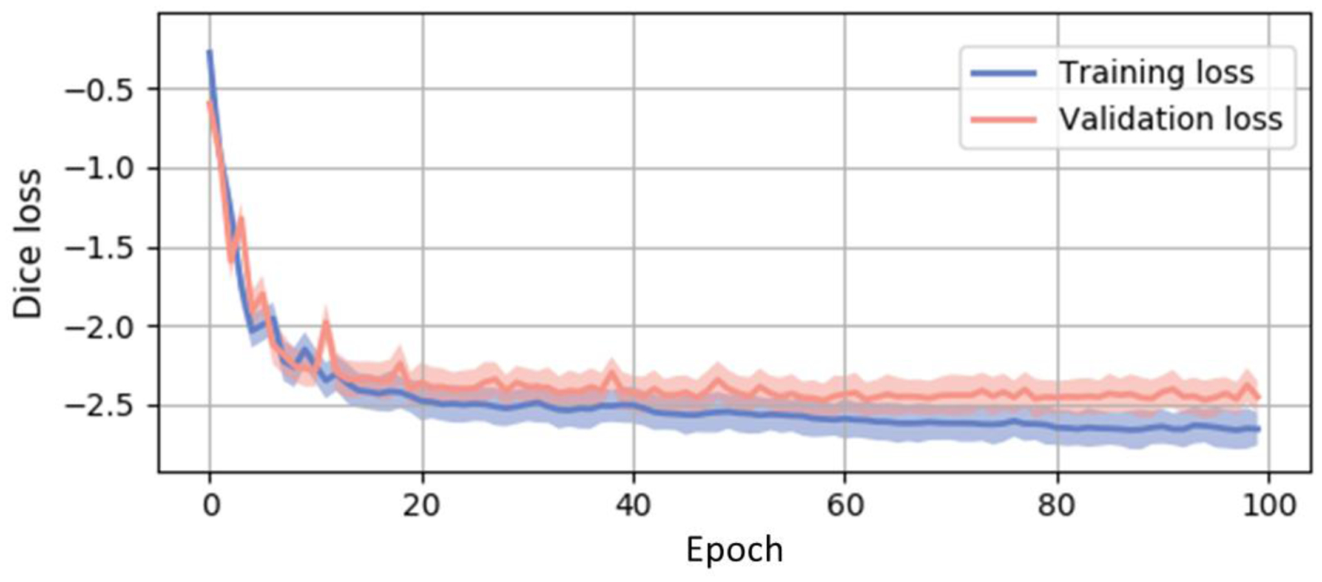
Training and validation curves acquired from averaging lossed from five-fold experiments. The shadows show the variance of these trainings and validations. The Dice loss is summarized from all three classes. The curve shows consistent sensitivity across data folds and our multi-categorical segmentation model.

4. CONCLUSION

In this paper, we study a challenging problem of multi-label renal segmentation, including the cortex, the medulla and the pelvicalyceal system. This task is crucial in identifying renal structures and functions with clinically acquired CT images. Our main contribution in this work is that 1) we retrieved and identified data from 45 patients, manually annotated right and left kidney structures and 2) employed a patch-based method for automatically segmenting renal structures. Shown in Figures 4 and 5, both the mean and the median Dice scores of the 20 external testing scans increased from the baseline segmentation model to the proposed algorithm on the cortex, the medulla and pelvicalyceal system. While the proposed algorithm yields substantive improvement of performance over the baseline under prospective evaluation, further exploration could be undertaken to further refine segmentation especially regarding small tissues of the calyx and pelvis. In the future, we would like to test our method on the subjects with pathological conditions. The investigation of clinically acquired pathology subjects will be worthy of interests

REFERENCES

- [1].Lee VS, Rusinek H, Noz ME, Lee P, Raghavan M, and Kramer EL, “Dynamic three-dimensional MR renography for the measurement of single kidney function: initial experience,” Radiology, vol. 227, pp. 289, 2003. [DOI] [PubMed] [Google Scholar]
- [2].Halpern EJ et al. , “Preoperative evaluation of living renal donors: comparison of CT angiography and MR angiography,” Radiology, vol. 216, pp. 434, 2000. [DOI] [PubMed] [Google Scholar]
- [3].Sahani DV et al. , “Multi–detector row CT in evaluation of 94 living renal donors by readers with varied experience,” Radiology, vol. 235, no. 3, pp. 905–910, 2005. [DOI] [PubMed] [Google Scholar]
- [4].Abrams P, Urodynamics. Springer, 2006. [Google Scholar]
- [5].Takazawa R, Kitayama S, Uchida Y, Yoshida S, Kohno Y, and Tsujii T, “Proposal for a simple anatomical classification of the pelvicaliceal system for endoscopic surgery,” Journal of Endourology, vol. 32, pp. 753,2018. [DOI] [PubMed] [Google Scholar]
- [6].Bae KT, “Intravenous contrast medium administration and scan timing at CT: considerations and approaches,” Radiology, vol. 256, no. 1, pp. 32–61, 2010. [DOI] [PubMed] [Google Scholar]
- [7].Tang Y et al. , “Contrast Phase Classification with a Generative Adversarial Network,” arXiv preprint arXiv:1911.06395, 2019. [DOI] [PMC free article] [PubMed] [Google Scholar]
- [8].Chen X, Summers RM, Cho M, Bagci U, and Yao J, “An automatic method for renal cortex segmentation on CT images: evaluation on kidney donors,” Academic radiology, vol. 19, no. 5, pp. 562–570, 2012. [DOI] [PMC free article] [PubMed] [Google Scholar]
- [9].Shen W, Kassim AA, Koh H, and Shuter B, “Segmentation of kidney cortex in MRI studies: a constrained morphological 3D h-maxima transform approach,” International Journal of Medical Engineering and Informatics, vol. 1, no. 3, pp. 330–341, 2009. [Google Scholar]
- [10].Li X et al. , “Renal cortex segmentation using optimal surface search with novel graph construction,” in International Conference on Medical Image Computing and Computer-Assisted Intervention, 2011: Springer. [DOI] [PMC free article] [PubMed] [Google Scholar]
- [11].Chevaillier B, Ponvianne Y, Collette J-L, Mandry D, Claudon M, and Pietquin O, “Functional semi-automated segmentation of renal DCE-MRI sequences,” in 2008 IEEE International Conference on Acoustics, Speech and Signal Processing, 2008: IEEE, pp. 525–528. [Google Scholar]
- [12].Shim H, Chang S, Tao C, Wang JH, Kaya D, and Bae KT, “Semiautomated segmentation of kidney from high-resolution multidetector computed tomography images using a graph-cuts technique,” Journal of computer assisted tomography, vol. 33, no. 6, pp. 893–901, 2009. [DOI] [PubMed] [Google Scholar]
- [13].Tang Y, Jackson HA, De Filippo RE, Nelson MD Jr, and Moats RA, “Automatic renal segmentation applied in pediatric MR Urography,” Int. J. Intell. Inf. Process, vol. 1, no. 1, pp. 12–19, 2010. [Google Scholar]
- [14].Çiçek Ö, Abdulkadir A, Lienkamp SS, Brox T, and Ronneberger O, “3D U-Net: learning dense volumetric segmentation from sparse annotation,” in International conference on medical image computing and computer-assisted intervention, 2016: Springer, pp. 424–432. [Google Scholar]
- [15].Thong W, Kadoury S, Piché N, and Pal CJ, “Convolutional networks for kidney segmentation in contrast-enhanced CT scans,” Computer Methods in Biomechanics and Biomedical Engineering: Imaging & Visualization, vol. 6, no. 3, pp. 277–282, 2018. [Google Scholar]
- [16].Xu Y et al. , “Outlier Guided Optimization of Abdominal Segmentation,” arXiv preprint arXiv:2002.04098, 2020. [DOI] [PMC free article] [PubMed] [Google Scholar]
- [17].Zhou Y et al. , “Semi-Supervised Multi-Organ Segmentation via Deep Multi-Planar Co-Training,” arXiv preprint arXiv:1804.02586, 2018. [Google Scholar]
- [18].Chu C et al. , “Multi-organ segmentation based on spatially-divided probabilistic atlas from 3D abdominal CT images,” in International Conference on Medical Image Computing and Computer-Assisted Intervention, 2013: Springer, pp. 165–172. [DOI] [PubMed] [Google Scholar]
- [19].Roth HR et al. , “Hierarchical 3D fully convolutional networks for multi-organ segmentation ,” arXiv preprint arXiv:1704.06382, 2017. [Google Scholar]
- [20].Xu X, Zhou F, Liu B, Fu D, and Bai X, “Efficient Multiple Organ Localization in CT Image using 3D Region Proposal Network,” IEEE transactions on medical imaging, 2019. [DOI] [PubMed] [Google Scholar]
- [21].Lin D-T, Lei C-C, and Hung S-W, “Computer-aided kidney segmentation on abdominal CT images,” IEEE transactions on information technology in biomedicine, vol. 10, no. 1, pp. 59–65, 2006. [DOI] [PubMed] [Google Scholar]
- [22].Roth HR et al. , “A multi-scale pyramid of 3d fully convolutional networks for abdominal multi-organ segmentation,” in International Conference on Medical Image Computing and Computer-Assisted Intervention, 2018: Springer, pp. 417–425. [Google Scholar]
- [23].Tang Y et al. , “Improving splenomegaly segmentation by learning from heterogeneous multi-source labels,” in Medical Imaging 2019, vol. 10949: International Society for Optics and Photonics, p. 1094908. [DOI] [PMC free article] [PubMed] [Google Scholar]