Clusters of ultrasound scattering parameters for the classification of steatotic and normal livers

Abstract

The study of ultrasound tissue interactions in fatty livers has a long history with strong clinical potential for assessing steatosis. Recently we proposed alternative measures of first and second order statistics of echoes from soft tissues, namely the H-scan that is based on a matched filter approach to quantify scattering transfer functions and the Burr distribution for modeling speckle patterns. Taken together, these approaches produce a multi-parameter set that is directly related to the fundamentals of ultrasound propagation in tissue. To apply this approach to the problem of assessing steatotic livers, these analyses were applied to in vivo rat livers (N = 21) under normal feeding conditions or after receiving a methionine and choline deficient (MCD) diet that produces steatosis within a few weeks. Ultrasound data was acquired at baseline and again at weeks 2 and 6 before applying the H-scan and Burr analysis. Furthermore, a classification technique known as the support vector machine (SVM) was then utilized to find clusters of the five parameters that are characteristic of the different steatotic liver conditions as confirmed by histologic processing of excised liver tissue samples. With the in vivo multiparametric ultrasound measurement approach and determination of clusters, steatotic vs. normal livers can be discriminated with 100% accuracy in a rat animal model.

INTRODUCTION

The non-invasive quantification of liver fat is an emerging imperative as fatty liver diseases continue to increase around the world (Jennings et al. 2018). Measures of steatosis that can be incorporated into imaging platforms are desirable and have received extensive attention (Goceri et al. 2016; Ozturk et al. 2018). Ultrasound techniques are attractive because they could provide a relatively inexpensive, rapid, and widely available means for assessing liver steatosis. There is not yet a consensus agreement on the change in ultrasound propagation and scattering from normal to steatotic livers, even as more parameters can now be measured in clinical settings. In parallel, there remains some uncertainty as to the most appropriate physical and mathematical models of scattering from the normal and diseased tissues. Nonetheless, earlier pioneering work on the use of multiparametric clusters of ultrasound-related measurements have shown promise (Momenan et al. 1987; Momenan et al. 1994).

Recent published results are reasonably aligned with a longstanding hypothesis that the accumulation of fat in liver will increase the viscous (lossy) attenuation, and decrease the speed of both ultrasound (longitudinal) and shear waves (Freese and Lyons 1977; Narayana and Ophir 1983; Maklad et al. 1984; Lin et al. 1987; Parker et al. 1988; Lu et al. 1999; Ghoshal et al. 2012; Barry et al. 2014; Barry et al. 2015; Parker et al. 2018; Sharma et al. 2019; Wernberg et al. 2020; Jeon et al. 2021). Related to this, the accumulation of fat-filled vesicles increases the scattering. Thus, as fat increases within an otherwise normal liver, we would expect to see attenuation increase, along with some measures of ultrasound scattering (Maklad et al. 1984; Taylor et al. 1986; Parker et al. 1988). An overview of different strategies for characterizing steatosis with ultrasound systems is found in Pirmoazen et al. (2020).

Traditional measures of scattering include the frequency dependence of scattering and the first order statistics of speckle formed by the returning ultrasound echoes. There are a variety of approaches to these, but recently a re-examination of the physics of pulse-echo ultrasound scattering from tissues has resulted in the emergence of H-scan (Parker 2016; Parker and Baek 2020) and the Burr speckle analysis (Parker 2019a; Parker 2019b; Parker and Poul 2020a; Parker and Poul 2020b). These approaches extract key metrics from the returning ultrasound echoes and are tied directly to models of scattering dominated by the fractal branching vasculature in normal tissues. In a recent study of H-scan and Burr analyses applied to animal models of primarily fibrosis and inflammation, the multiparametric clusters representing normal and pathological states were found to be well separated with a resulting 94% classification accuracy (Baek et al. 2020b). The potential usefulness of the multiparametric clusters for steatosis as a distinct clinical problem motivates this study.

In parallel with the growth of ultrasound metrics, there have been recent machine learning results classifying liver states. These focus more on utilizing learning tools with log-compressed B-scan ultrasound images and employ image processing measures as the input to the classifiers, which are not specific to ultrasound signals. A support vector machine (SVM) classifier for liver (Virmani et al. 2013) used a two-dimensional (2D) wavelet packet transform for the log-compressed data to generate the inputs that were standard deviation, mean, and energy. A liver classifier using texture analysis (Singh et al. 2014) used the gray scale images to extract features based on contrast, roughness, and homogeneity, etc. A steatosis classifier (Byra et al. 2018) used SVM for classification, but to extract features for the classifier’s input, a deep convolutional neural network was employed with log-compressed B-scan ultrasound images. A steatosis classification study (Andrade et al. 2012) compared the performance of three different classifiers: artificial neural network (ANN), SVM, and k-nearest neighbors (kNN). The study concluded that SVM had the best performance in terms of accuracy. However, the study also used B-scan ultrasound images to extract input features, which can characterize the echogenicity, including a gray level run length matrix, co-occurrence, texture energy, and other measures of image statistics. Therefore, liver classification research often relies on B-scan ultrasound images to extract different features and then employs the more recently developed machine learning techniques for decision making. However, B-scan ultrasound images are easily changed by users due to their preference of scan settings; the textures of these images also vary depending on post-processing methods and the envelope contains much less information than the raw radiofrequency (RF) ultrasound signals.

Our study employs principal component analysis (PCA) and SVM as a state-of-art machine learning approach. PCA provides a well-established framework for linear combinations of multiple parameters (Pearson 1901) and is useful for clustering and reducing the dimensionality of the data set. The SVM is a robust supervised learning classification technique that has the ability to define nonlinear classification boundaries on multidimensional measurements (Vapnik 1999). In our case, measurements are based on features from RF signals derived from recent models that are intimately related to physics of ultrasound.

To apply these to the detection of liver steatosis, we first examine relevant theoretical models of scattering that are likely to be dominant in cases of normal and steatotic liver tissues. Secondly, the effect of these scattering models on the returning ultrasound echoes are examined in terms of their first order statistics (i.e., histogram of echo amplitudes) and second order statistics (i.e., backscatter vs. frequency). Using animals fed a normal or special diet that results in a progressive accumulation of liver fat, we thirdly examine echoes from rat livers using a high-frequency ultrasound scanner. Finally, a SVM is implemented on principal components of the ultrasound scattering measurements to classify clusters in multiparametric space.

Together, these elements work towards a mathematical framework for determining multiparametric signatures of ultrasound echoes from the normal liver as compared with those from increasingly steatotic liver conditions.

THEORY

Scattering models for normal and steatotic livers

Early studies on ultrasound scattering from normal livers established some consistent results (Chivers and Hill 1975; Gramiak et al. 1976; Bamber 1979; Zagzebski et al. 1993). Backscatter was found to increase with frequency, an f^1.4 power law behavior (Campbell and Waag 1984) over the low MHz imaging band. The first-order statistics of liver echo amplitudes were found to resemble optical speckle patterns (Burckhardt 1978). Some established theories postulated scattering from spheres or spherical correlation functions, usually correlated to cell size and shapes (Lizzi et al. 1983; Insana et al. 1990). As a recent alternative we postulated that normal tissue scattering is influenced by the impedance mismatch between the fractal branching vascular tree, and the parenchyma comprised of mostly close-packed hepatocytes in the case of the liver. Within this model the mathematics of speckle and scattering are not attributed to random points or spheres, but rather the scattering from cylinders and fractal branching structures (Parker 2019a; Parker 2019b; Parker et al. 2019) as depicted in Figure 1. Importantly the frequency dependence of ultrasound backscatter and the probability distribution function for speckle amplitudes from the fractal branching vasculature are dominated by a power law relationship related to the fractal dimension D.

Figure 1.

Schematic of a first order approximation for superposition of scattering sites in simple steatosis. At the right side are shown the dominant scattering structures from the normal liver rendered from a micro-CT contrast-enhanced 3D rendering of the vasculature within a mouse liver. In normal liver, the weak ultrasound scattering from the fluid-filled vasculature is a major source of returning echoes. Accumulating fat vesicles add to the scattering and produce a change in received echoes as compared with the normal liver.

In early stages of fat accumulation in the liver, microvesicles and macrovesicles appear as small randomly positioned spheres (many are below 40 microns), and since these have a different acoustic impedance compared to the surrounding hepatocytes, are a source of scattering. Traditional long-wavelength (Rayleigh scattering) models would predict ultrasound backscatter intensity increasing as f⁴ power from random small spheres, which in the simplest model would be additive to the baseline scattering found in the normal liver. However, this simplified model shown in Figure 1 may not apply to advanced stages where the distribution of fat can become zonal, concentrating in periportal patterns (Schwen et al. 2016). Also, the chemical composition of fat in later stages can be altered (Peng et al. 2015; Chiappini et al. 2017), so both the size distribution and the scattering strength may vary with advanced stages beyond simple steatosis. In these cases pronounced clustering across different length scales from the smallest microvesicles to the larger portal structures could then resemble a fractal clustering structure (Javanaud 1989; Shapiro 1992), which then would approach a lower power law compared to a Rayleigh scattering model.

Assessment with H-scan and Burr parameters

In this study, we explore ultrasound scattering metrics derived from the H-scan (a matched filter approach) images along with histograms of speckle amplitude. Further details of these approaches are described in the Methods section, and the combined analyses produce five measured parameters related to ultrasound scattering structures. Under our hypothesis of additive scattering (Figure 1), most parameters are expected to increase as a consequence of the addition of Rayleigh scattering sites, producing multiparametric clusters that are separated from normal values. The degree of separation can be visualized and quantified using PCA and the SVM. These steps are detailed in later sections.

METHODS

Study design and animals

This protocol was approved by the Institutional Animal Care and Use Committee (IACUC) at the University of Texas at Dallas. As shown in Figure 2, an in vivo study with 21 Sprague-Dawley rats (Charles River Laboratories, Wilmington, MA) was designed to investigate fat accumulation in the liver. The methionine and choline deficient (MCD) diet, which is a common dietary model for nonalcoholic fatty liver disease (NAFLD), induced steatosis. The enrolled animals were randomly divided into two groups, namely, control (N = 9) or diet (N = 12). The diet group was fed the MCD diet (MP Biomedicals, Solon, OH); it is high in sucrose and fat (40% sucrose and 10% fat), but deficient in methionine and choline. All animals had free access to water and food under a 12-hour day-night cycle and were tracked for 6 weeks.

Figure 2.

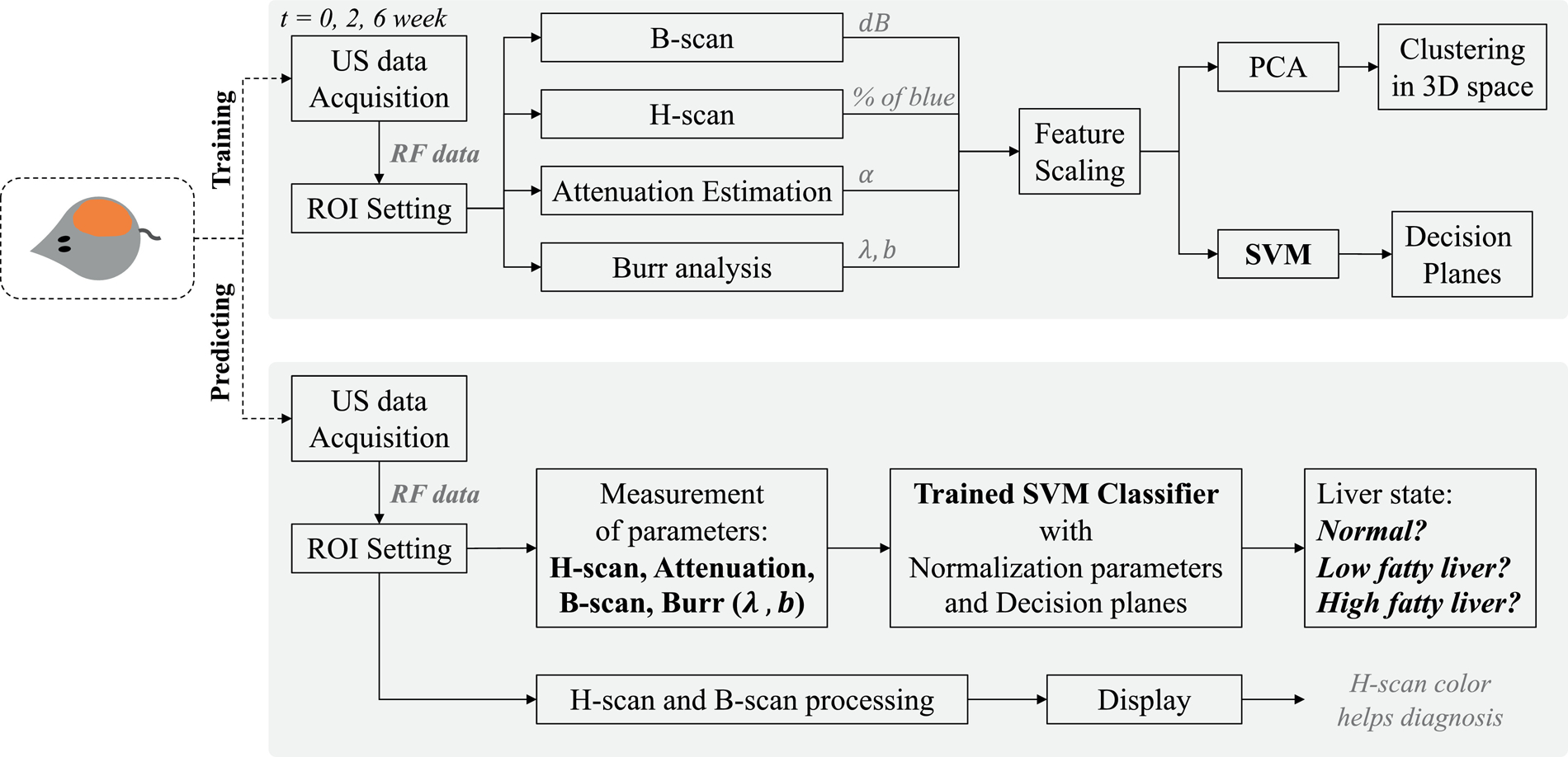
Study design: a liver steatosis diagnosing tool with SVM and H-scan imaging. The SVM was trained by using the 5 measured parameters from B-scan, H-scan, attenuation estimation, and Burr analysis, resulting in the SVM classifier for liver diagnosis. PCA using the parameters provided a reduced dimensionality view of clusters of normal, low fat, and high fat livers. H-scan imaging provides colors representing liver states, and the SVM provides the category of the input liver data. We note that SVM could also be performed on the reduced parameter space defined by PCA, with lower dimensionality.

Although the MCD diet is known to cause steatosis within weeks, three different types of histological stains were performed at the end of this study to detect the presence of steatosis and fibrosis, which can be induced during the various stages of NAFLD. The staining methods were Picro-Sirius red and hematoxylin and eosin (H&E).

All rats were scanned by using a high-frequency ultrasound scanner, (Vevo 3100, FUJIFILM VisualSonics, Toronto, Canada), equipped with a 15 MHz center frequency linear array transducer (MX 201). Liver scans were performed at weeks 0, 2, and 6, and RF data was acquired at a 240 MHz sampling rate from conventional line-by-line single focus scanning at 53 frames per second. All ultrasound scanning parameters and conditions were kept consistent, including the gain, focal depth, and transmit power throughout the study. Furthermore, all ultrasound RF data used for the H-scan and Burr analysis were acquired after time gain compensation (TGC) which was also held consistent throughout the study.

A square region-of-interest (ROI) was consistently set over time within the depth between 6 to 12 mm (size of ROI). We tried to include a lateral width with more scanlines, however areas with artifacts, vessels, or cysts were excluded. Within the ROIs, ultrasound measurements for B-scan, H-scan, attenuation estimation, and histogram Burr analysis were performed. The signal processing resulted in 5 parameters that were used to characterize liver states. After data normalization (feature scaling), parameters were assigned as inputs of a SVM classifier and were also used to visualize clusters representing 3 liver classes. Liver states were divided into the 3 classes of normal (baseline), low fatty, or high fatty livers. The normal group includes all control cases at all 3 study time points, and the diet group at week 0. This normal groups is hereafter referred to as “baseline”. The low and high classes are defined as MCD diet rats at 2 and 6 weeks, respectively.

H-scan ultrasound analysis

H-scan ultrasound has been designed to classify scattering transfer functions of tissues. (Parker and Baek 2020) and is based on the different power law transfer functions that influence frequency components in ultrasound echoes. In this H-scan implementation the received signals, r(t), are processed through a bank of matched filters by using a 256 Gaussian bandpass filter set for convolution with r(t):

$$\underset{n}{\text{max}}\left({\Im }^{-1}\left\{\Im (r(t))\cdot G_n(f)\right\}\right),$$ (1)

where G_n(f) is each Gaussian bandpass filter in the frequency domain, equally spaced over the bandwidth of the imaging system. By choosing the matched filter indexed by n that maximizes equation (1), the peak frequency of G_n(f) becomes the estimated frequency at time t of r(t) and is mapped into specific colors, meaning that H-scan is displayed as a pseudo-color mapping. However, ultrasound propagation accumulates frequency-dependent attenuation over depth, biasing the H-scan colors from more blue at near depth to more red at far depth. To avoid this bias, the attenuation-dependent color shift needs to be compensated.

Attenuation estimation and correction within the H-scan analysis

An ultrasound transmission pulse can be modeled by a bandpass Gaussian function of $e^{-{\left(f-f_0\right)}^2/2{\sigma }^2}$ with a center frequency of f₀ and bandwidth σ. A frequency- and depth-dependent attenuation term e^{−α fz} is then included to account for losses, whereby the frequency spectrum S(f) of the pulse can be written as:

$$S(f)=e^{-\frac{{\left(f-f_0\right)}^2}{2{\sigma }^2}}\cdot e^{-\alpha \mathit{\text{ fz}}},$$ (2)

where f is the frequency in MHz, α is the attenuation coefficient in Np/cm/MHz, and z is depth in cm. The attenuation of an ultrasound signal causes a decrease in the peak frequency, which can be estimated by taking the first partial derivative with respect to f and finding its zero at peak frequency f_p resulting in:

$$\widehat{\alpha }(z)=-\frac{f_p(z)-f_0}{z\cdot {\sigma }^2},$$ (3)

where f_p(z) is the peak frequency measured using H-scan ultrasound and is averaged over all scan lines within the ROI, as shown in Figure 3.

Figure 3.

Schematic for H-scan. For each frame, the attenuation coefficient is estimated, and using this coefficient attenuation correction was performed. The corrected RF data without frequency shift caused by attenuation was assigned as an input of H-scan.

The TGC applies a broadband gain (pre-set by an experienced operator for the animal livers) that increases with depth, but this is not sufficient to compensate for the frequency dependence of attenuation, which is most pronounced at the higher frequencies within the transmit pulse’s spectrum. The estimated $\widehat{\alpha }$ from equation (3) was input to a digital inverse filter which is applied for frequency-dependent attenuation correction at increasing depths. The inverse filter simply boosts the higher frequencies relative to the lower (less attenuated) frequencies over varying depths, and more details for the correction can be found in (Baek et al. 2020a; Baek et al. 2020b; Parker and Baek 2020). Consequently, corrected RF signals compensated for attenuation effects were used to produce the H-scan ultrasound images.

The final parameters that were evaluated within each liver ROI included echogenicity or brightness (dB) for B-scan, α reported herein with a conversion to the more commonly used units of dB/cm/MHz for attenuation, and percent of blue for H-scan. B-scan ultrasound echogenicity was calculated from log-compressed data where 0 dB is set to the same brightness level for all scans. The attenuation was measured by averaging eqn (3) over depth. 256 color levels were used for the H-scan image format, which changes from red to black to blue in sequence, represented by a color bar in Figure 5. Red and blue pixels are equally divided into the pixels with color levels C_i of [1, 128] and [129, 256], respectively, which can be converted into normalized color intensity I_i:

$$I_i=\frac{|C_i-128.5|}{127.5}\text{ ,}$$ (4)

where i is the index of each pixel. The number of red and blue pixels are written as n_R and n_B, respectively, and then the percent of blue (% of blue) is defined by:

$$\text{\% of blue }=\frac{n_B}{n_R+n_B}\times 100\text{\%}$$ (5)

Figure 5.

Scans of one rat in the MCD diet group. Top row: B-scan; second row: H-scan images; third row: % of blue or red profile. The bottom row shows Burr-fitting to histogram at weeks (a) 0, (b) 2, and (c) 6, with vertical axis representing the probability P of amplitude A (horizontal axis A in arbitrary units). The images and histograms are all from the same rat in the diet group. With the accumulation of fat, the H-scan blue channel (high frequency, corresponding to small scatterers) output increases, as does the Burr b and λ parameters.

First-order statistics of speckle and the Burr distribution

The histogram of ultrasound echo amplitude A for the normal liver speckle pattern is governed by a two parameter probability density function (PDF), N_n(A) according to a novel framework proposed by Parker (2019a; 2019b) and employed in (Baek et al. 2020b; Parker and Poul 2020a; Parker and Poul 2020b). Based on this new framework, speckle patterns of the normal liver stems from the fractal network of fluid-filled vessels with a size distribution following a power law function as N(a) = N₀/a^b, where N₀ is the number density of vessels within the organ, a is vessel radius, and b is the key fractal power law parameter. Within reasonable approximations concerning pulse echo imaging of the vascular beds, the probability density function for echo amplitudes A is given by:

$$N_n[A]=\frac{2A(b-1)}{{\lambda }^2{\left[{\left(\frac{A}{\lambda }\right)}^2+1\right]}^b},$$ (6)

where λ is related to system factors like amplifier gain and a minimum vessel size of the fractal network, and b to the fractal vessel network. Equation (6) is derived by using a 3D convolution model and happens to be a Burr type XII distribution proposed for general applications unrelated to medical imaging in the 1940s (Burr 1942). More detail on the derivation is found in (Parker 2019a).

Variation in scattering structures and spacing within soft tissues produce changes in the value of Burr parameters b and λ, which are estimated by fitting a Burr distribution to the normalized histogram of tissue speckle amplitude. Thus, the two Burr parameters are estimated for liver tissues of control and diet groups of rats in the present study at three different weeks. The ROI for obtaining the speckle amplitude distribution in each rat liver is selected in a uniform region devoid of large anechoic vessel areas.

Histogram fitting is done in MATLAB (MathWorks, Inc., Natick, MA) using a nonlinear least squares minimization of error. By using additional estimates of the two parameters from the mode and median equations, some bounds are placed on the Burr fitting parameters. The results give the smallest set of b and λ as estimated parameters, consistent with eqn (6) and with an R² value of higher than 99.8% for each frame of each liver scan.

The SVM classifier

The SVM is one of the supervised learning approaches to construct hyperplanes that classify multidimensional data into several classes (Cortes and Vapnik 1995; Vapnik 1999; Bishop 2006), which is a convex optimization problem given by:

$$\text{minimize}\left(\frac{1}{2}{\Vert \overrightarrow{w}\Vert }^2+C\sum _{n=1}^N{\xi }_n\right)$$ (7)

where $\overrightarrow{w}$ is the vector describing the hyperplane of data points x_n represented as $\overrightarrow{w}\cdot x_n+b$, and ξ_n is the penalty for misclassified points. To construct a SVM, the box constraint C and σ of a Gaussian kernel were optimized. The first term of eqn (7) denotes maximizing the margins between the classes during training, subsets of data near the class boundaries are used as support vectors whose index are n in eqn (7). The training allows misclassified points with the penalty of ξ_n, and therefore more robust classification with smooth hyperplanes can be performed preventing overfitting. As this formulation is a convex optimization problem with an optimal solution, the SVM can avoid local minima. Moreover, Gaussian kernels enable SVM to set non-linear hyperplanes, with the shape of the hyperplane dependent on the setting parameter of σ. Due to the advantages, a SVM with Gaussian kernels was used to classify liver states based on the ultrasound scattering signatures characterized by H-scan, B-scan, attenuation and the Burr analysis. The study design shown in Figure 2 illustrates the proposed SVM training and prediction procedures which were implemented in MATLAB. The SVM classifier was trained first with parameters from a total of 1,877 data sets, including 1,175 normal, 342 low fat, and 360 high fatty liver cases. These parameters were estimated from the raw ultrasound RF echoes acquired from the 21 rats and with approximately 30 frames for each liver scan.

Every case has the five parameters of % of blue from H-scan, α from attenuation, dB scale intensity from B-scan, b, and dB scale λ from the Burr analysis. However, these parameters have different data ranges and scales, which could have a different impact on processing; the larger the scale of a feature, the more weight it can carry compared to other smaller scale features. Thus, data normalization was performed before the features were put into the SVM training. Z-score normalization (Jayalakshmi and Santhakumaran 2011) was used as the most commonly used data normalization technique, of which normalized data z is given by:

$$z=\frac{x-{\mu }_{\text{baseline}}}{{\sigma }_{\text{baseline}}},$$ (8)

where x is raw data from the measurements, and μ_baseline and σ_baseline are the average and standard deviation of base line data for each input feature, respectively. In other words, this study used only baseline cases to set zero mean and unit variance, whereby the data distribution can show how the data of disease cases differ from those of normal.

The 5 normalized features were set to the inputs for the SVM training and each dataset has its tag among the three classes: normal, low fatty, and high fatty liver. Then, SVM training can construct hyperplanes, which can be used as decision planes for any other input with the 5 features. Thus, the trained SVM can classify liver states for unknown new inputs. Further details for implementation of the SVM classifier can be found in Baek et al. (2020b). In addition to SVM, PCA was performed to investigate the relative importance of the contribution from each parameter for classification. Furthermore, PCA is a useful tool to reduce the dimensionality of parameter space (from 5D in our case) in order to visualize the clusters and hyperplanes in 2D or three-dimensional (3D) space. In order to examine the hyperplanes in 2D and 3D space, the first 2 and 3 PCs were used as inputs to construct SVM classifiers exclusively for visualization, respectively. Note that the liver classification of this study in Figure 2 used the 5 features without first applying PCA since we only have 5 parameters and those are treated as essentially independent parameters. Generally, PCA as a pre-processing of machine learning is useful when the number of inputs is large and there is dependency between the input data; more than 20 parameters is reported as a large set that benefits from PCA (Howley et al. 2006). Otherwise, PCA can cause information loss with a drop in classification performance.

RESULTS

Histological sections confirmed that high grade steatosis was induced only in the MCD diet group. These livers displayed significant amounts of accumulated fats, with minimal inflammation and no evidence of other diseases. Examples of histology are shown in Figure 4. We scored the percentage of fat area to the entire tissue area in selected histology images; 3 control and 6 diet cases were enrolled. The histology images were binarized, and then the bright areas were counted as fat. The detected fat areas are illustrated in green color in Figure 4(g) and (f). The percentages of fat area were measured as 0.06 ± 0.07% (mean ± standard deviation) and 29.93 ± 8.82% for the control and diet groups (p-value of 0.008). A steatosis quantifying study (Munsterman et al. 2019) demonstrated the positive correlation between steatosis grade and the percentage, reporting that grade 3 steatosis corresponds to 16% fat in human liver, which is lower than this study. Therefore, we confirmed that week 6 rats have severe steatosis.

Figure 4.

Histology images of liver sections stained with Picro-Sirius red for steatosis. Object scale (a–c) and 10× object virtual magnification (d–f) are shown. (a) and (d) represent a control case, (b) and (e) represent a 6 week diet case; (c) and (f) show another 6 week diet liver. Fat accumulation can be seen in MCD diet cases. An analysis of fat is shown in the bottom row. For the case in (e), a box ROI was selected as shown in (g), showing the detected fat vesicles with green color. The ROI of (g) is magnified into (h) and (i); (h) only shows the histology image before fat detection, and (i) shows detected fat with green color.

The enrolled 21 rats were scanned by ultrasound at 0, 2, and 6 weeks. Figure 5 shows examples of B-scan, H-scan % of blue profile, and Burr-fitting results from one rat in the diet group, highlighting the progression of fat accumulation. ROIs for processing are indicated by the red boxes on top of the B-scan ultrasound images, of which depth ranges from 6 to 12 mm. Additionally, Figure 6 shows the progression of the measurements over time and statistical plots between the three groups: normal, low (week 2 diet), and high (week 6 diet) fatty liver. The following statistical notations were employed: ns (no significance) p > 0.05; * p < 0.05; ** p < 0.01; *** p < 0.001; and **** p < 0.0001.

Figure 6.

The progression of fat accumulation over time (left column) and statistics (right column) of the five measurements: B-scan intensity, H-scan percent blue (indicating a shift to smaller scatterers), attenuation, Burr λ, and Burr b.

B-scan, H-scan, and Burr parameters

As fat accumulated in the animal livers over time, B-scan and H-scan ultrasound images in Figure 5 show the changes in brightness and color, respectively. The B-scans at 6 weeks are brighter than those at 0 and 2 weeks; otherwise, the early stage fatty case at 2 weeks has comparable brightness with normal. However, H-scan ultrasound imaging results indicate that the blue colors increase more steadily over time compared with color changes for early stage liver steatosis at 2 weeks. These trends are consistently shown for the quantitative measurements in Figures 6 (a) and (c). The third row in Figure 5 represents the % of blue profiles, which were acquired after attenuation correction. The attenuation estimates used were 0.55, 0.61, and 0.70 dB/MHz/cm for the representative cases at weeks 0, 2, and 6, respectively.

The measurements obtained from the control group remained essentially unchanged, but those from the diet group increased over time, indicating fat accumulation in the liver. Moreover, the estimates of the attenuation coefficient in Figure 6(e) have similar progression to the H-scan; the estimated attenuation coefficient of the control group remains constant (approximately 0.5 dB/MH/cm), while that of the diet group continues increasing over time without any delay within the early stage growth of fat. Accordingly, H-scan ultrasound and attenuation estimation as frequency-dependent analyses monitor the progression of fat accumulation in liver over time and appear to be more sensitive than the echo intensity-dependent analyses, including B-scan ultrasound and the Burr analysis.

Figures 6 (b), (d), and (f) show the statistical results for B-scan intensity, H-scan, and attenuation estimation, respectively. The three groups were included: normal, low fatty liver, and high fatty livers. There is statistical difference between the three groups (p < 0.0001), meaning that three different liver states’ distributions can be discriminated by these measurements. Considering the data distribution based on the half-violin and box plots, the H-scan ultrasound has the least overlap area between the liver states among the 5 measurements. Quantitatively, the H-scan percentage of blue for the diet group at 6 weeks is 79.2% within the range of 100%, and the control group has a value of 50.6%, whereby this measurement can also explain the fat accumulation clearly. Similarly, the attenuation coefficient for the diet group at 6 weeks is 0.74 dB/MHz/cm, and the average for the control group is 0.50 dB/MHz/cm. Moreover, to evaluate the data distribution, the coefficient of variation (σ/|μ| where σ and μ are standard deviation and mean, respectively) was calculated: 0.024 and 0.050 for H-scan and attenuation for the diet group at 6 weeks, respectively. Larger values of 0.894, 0.725, and 0.138 were obtained for the other 3 measurements of B-scan, Burr λ, and b, respectively.

Finally, the Burr parameters are shown in Figures 6 (g–j), demonstrating a trending increase in both the b and λ parameters with time in the MCD diet group, whereas the control group remains relatively unchanged.

Multidimensional clusters and the SVM-based classifier

The SVM-based liver state classifier was implemented, and consequently the decision planes for predicting liver states were produced with 100% of classification accuracy as shown in Figure 7. The two optimized parameters of the classifier are 1 and 10 for the box constraint C and σ, respectively. The parameters were decided according to their accuracy and the shape of hyperplanes. Although any SVMs can allow misclassified data points near the boundaries of classes to set more robust hyperplanes, the proposed SVM of this study does not need to include wrong-placed data since this study’s features provide well-separated clusters in Figures 7(c) and (d). Therefore, C was minimized within the C range in MATLAB options, meaning that the training almost only maximizes the margin between the classes while SVMs are designed to maximize the margin and minimize the penalty of wrong-placed data. With a C of 1, σ of the Gaussian kernel was optimized within the range of 1 to 50 by investigating hyperplanes and accuracy. The smaller values of σ near 1 caused overfitting with 100% accuracy, but the larger values near 50 resulted in inaccurate hyperplanes that were close to linear shaped surfaces with 95% accuracy, indicating underfitting. Thus, 10 of σ was selected to provide smooth hyperplanes and 100% accuracy as shown in Figure 7(e). Additional details of the SVM optimization procedure are found in Baek et al. (2020b).

Figure 7.

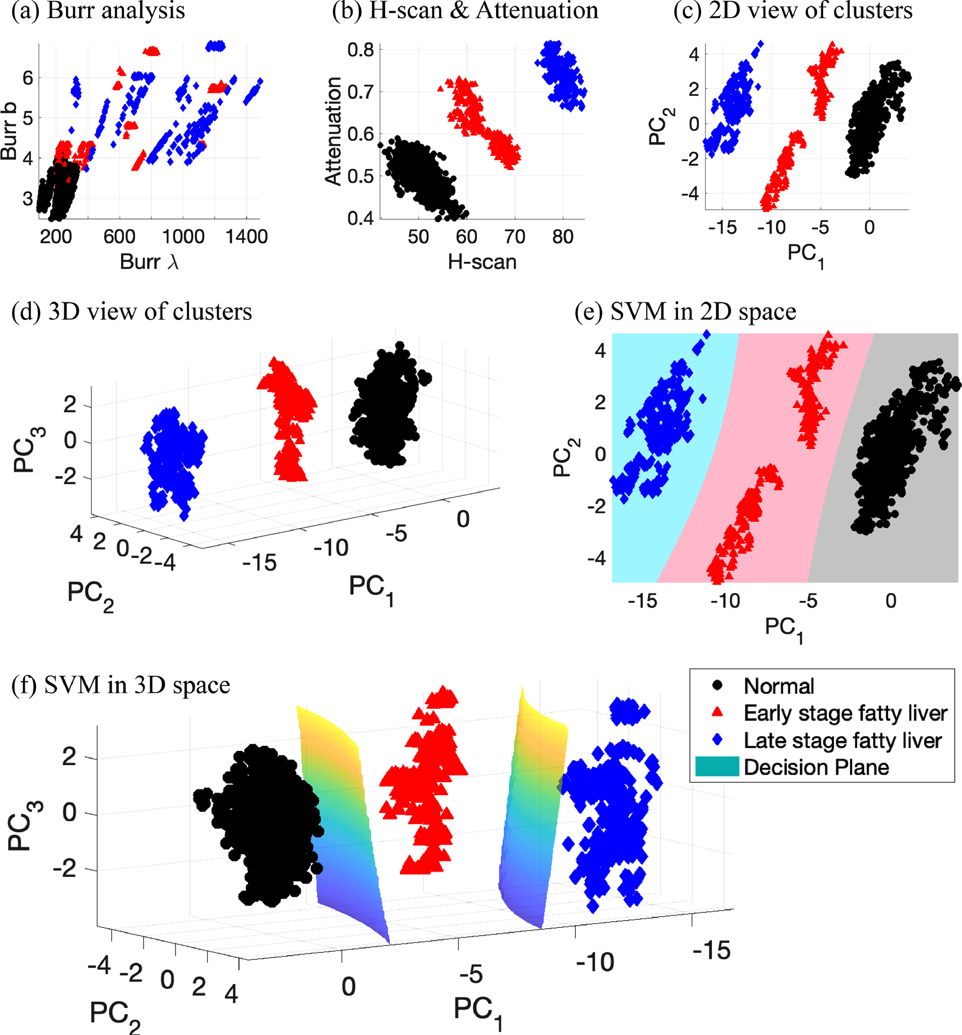
View of clusters and classification. (a) and (b) show clusters in 2D space from selected parameters from Burr and H-scan analyses. (c) 2D view of clusters by using the first and second principal components obtained from the 5 measurements: Burr λ and Burr b, H-scan, attenuation, and B-scan. (d) 3D view of clusters from the first three principal components. (e) and (f) SVM classification results in 2D and 3D space, respectively. (e) and (f) add the decision hyperplanes generated by SVM. The SVM results with 2D and 3D input have 100% of classification accuracy, which demonstrates this study’s measurements can provide clear discrimination between normal, low fatty, and high fatty liver.

To visually examine the hyperplane shapes or clusters of data set, reduced dimensions were considered since the employed features have five dimensions that cannot be visualized in 3D space. The five dimensions were reduced into two or three dimensions using PCA, as depicted in Figures 7(c) and (d). Data normalization steps for PCA from the raw data are given in Figure 8. Figure 8(a) presents raw data of the 5 features in this study with different scales, and the feature scaling step of Z-score resulted in the normalized data in Figure 8(b). The consistent distributions for normal data over the 5 features were obtained, and relative data positions of fatty cases can be compared between the features, demonstrating an increase in the measurements. H-scan ultrasound provided the highest measurement values for the 6-week diet group and the lowest overlaps between the three classes. The estimated attenuation coefficients demonstrate a steady increase along with fat accumulation, although there are more overlaps than H-scan, but less than the other three features. Regarding the other three features from echo intensity, the measurements cannot sensitively track the fat accumulation, showing severely overlapped distributions. Finally, as shown in Figure 8(c), PCA was performed to access the combination of the 5 features, whereby the first PC results in the best separation of the classes compared with any other measured features. The individual contributions for each PC are shown in Figure 8(d), and the total contributions for all PCs are provided in Figure 8(e). H-scan ultrasound contributed the most with 28.2%, which is approximately 10% higher than any other features.

Figure 8.

Feature scaling and PCA results. (a) Raw data from the 5 measurement. (b) Normalized data after Z-score feature scaling. (c) Principal components (PC) after PCA. (d) Contribution for each PC from the 5 measurements. (e) Contribution for all PCs: H-scan contributes the most as 28.2% compared to the other 4 methods.

DISCUSSION

This study implemented the two different approaches to characterize and quantify the liver conditions, which were the Burr and H-scan analyses corresponding to ultrasound echo- and frequency-dependent investigations, respectively. The analyses derived the 5 parameters, whereby the proposed SVM liver classifier reached 100% of accuracy without any misclassified cases and overfitting, meaning that the clusters from the three groups are well separated. As shown in Figures 7(c) and (d), the view of clusters in 2D and 3D space already provided three clearly distinguished clusters.

To visualize the clusters and hyperplanes, only 2 and 3 PCs were used, of which PCA caused some loss of information when comparing the reduced parameters to five-dimensional input parameters; the 2D and 3D clusters solely contain 93.8% and 97.0% of variance retained, respectively, as described in Figure 8(c). Despite the loss of information, the classification accuracies of SVM are still 100% since the combined measurements are sensitive to the accumulation of fat. However, the extension of these techniques to human clinical liver studies will encounter additional challenges including varying abdominal wall thicknesses, deeper tissue ROIs, and lower frequencies. The attenuation correction at greater depths may suffer from poor signal-to-noise conditions. Furthermore, diseases can simultaneously exhibit more complicated conditions, including inflammation, fibrosis, and lesions, likely resulting in less perfect classification results. In these cases, the higher dimensional parameter spaces should be useful for identifying combinations of these pathologies. We expect that this study’s clear description for simple steatosis will help in discriminating the presence or absence of fat within complex liver pathology.

Figures 7(a) and (b) show clusters produced by scattering models from analysis of echo amplitudes and frequency, respectively: (a) Burr analysis; (b) H-scan and attenuation. Figure 7(a) from the Burr analysis shows that the clusters gradually moved from bottom left to top right due to fat accumulation. Therefore, normal and high fat cases are separable, and normal and low fat has mild overlaps, but almost all regions for low and high fat are overlapped. However, the analysis from H-scan and attenuation in Figure 7(b) obviously differentiates all clusters with adequate separation, using only two parameters to differentiate the three groups of livers. Extending the analysis further, Figures 7(c) and (d) provide clearly separable clusters, although the Burr analysis by itself contains overlap between the three groups. Including more information from independent approaches helps to track the changes in ultrasound signal.

When considering all of the assessment metrics in this study, including statistics, time progression, PCA, and machine learning, the H-scan parameters resulted in the best performance compared to the other features. However, the fusion of the 5 particular methods enhances the performance, whereby the margins between classes increased and clusters in multidimensional space shows better separation than those of only H-scan. In this sense, all the parameters contribute globally to the staging of steatosis, as presented in Figure 8(d). Furthermore, this approach using PCA and SVM can be extended to additional diagnostic measures as these become available.

The contributions for all PCs in Figure 8(e) from attenuation and Burr analysis are comparable near approximately 19% of contributions, but according to data distribution in Figures 8(a) and (b), attenuation has better discrimination with less overlap. Hence, the contribution percentages did not fully explain the results since the Z-score normalization only considers data distribution from all the given inputs without including class information. For instance, when a given data set has two input features with the same data distribution, but different overlaps between their classes, PCA considers them as the same input. Accordingly, as a future study, employing weights for better classified input features before PCA would help to discriminate the given classes with higher accuracies.

In summary, this study applies a unique combination of parameters related to scattering, attenuation, and first order statistics with the framework of the H-scan analysis, applied to steatosis using multiparametric clustering analyses. This extends the assessment of steatosis beyond emerging clinical ultrasound measures recently reviewed by Pirmoazen et al. (2020). We find that combinations of parameters enable better characterization and separation of normal livers from those with two progressive levels of fat accumulation, although any one measurement by itself is not sufficient. This multiparametric framework including H-scan, PCA, and SVM analyses creates an effective means to combine the different metrics for assessment of liver steatosis.

CONCLUSION

We applied the multiparametric H-scan and the Burr distribution analyses to study the steatosis in an animal model of NAFLD. These analyses derived five measured parameters that are directly linked to recent models of ultrasound–tissue interaction in normal and steatotic livers. We found that the H-scan ultrasound images and Burr parameters are individually sensitive to the accumulation of fat within the liver, with some degree of overlap found between different groups. However, when taken jointly the measured parameters formed well-separated clusters in five dimensional spaces and make possible a robust discrimination between controls, steatotic livers at 2 weeks, and those at 6 weeks. A PC and SVM classification approach was capable of discriminating between groups with a 100% accuracy. These strong results indicate potential use of this multiparametric approach in clinical studies of steatosis and its progression in humans.

References

- Andrade A, Silva JS, Santos J, Belo-Soares P. Classifier approaches for liver steatosis using ultrasound images. Proc Technol 2012;5:763–70. [Google Scholar]
- Baek J, Ahmed R, Ye J, Gerber SA, Parker KJ, Doyley MM. H-scan, shear wave and bioluminescent assessment of the progression of pancreatic cancer metastases in the liver. Ultrasound Med Biol 2020a;46:3369–78. [DOI] [PMC free article] [PubMed] [Google Scholar]
- Baek J, Poul SS, Swanson TA, Tuthill T, Parker KJ. Scattering signatures of normal versus abnormal livers with support vector machine classification. Ultrasound Med Biol 2020b;46:3379–92. [DOI] [PMC free article] [PubMed] [Google Scholar]
- Bamber JC. Theoretical modelling of the acoustic scattering structure of human liver. Acoust Lett 1979;3:114–9. [Google Scholar]
- Barry CT, Hazard C, Cheng G, Hah Z, Partin A, Chuang K, Mooney RA, Cao W, Rubens DJ, Parker KJ. Detection of steatosis through shear speed dispersion: a rat study. American Institute of Ultrasound in Medicine Annual Convention, 2014; [Google Scholar]
- Barry CT, Hazard C, Hah Z, Cheng G, Partin A, Mooney RA, Chuang KH, Cao W, Rubens DJ, Parker KJ. Shear wave dispersion in lean versus steatotic rat livers. J Ultrasound Med 2015;34:1123–9. [DOI] [PubMed] [Google Scholar]
- Bishop CM. Pattern recognition and machine learning, Chapter 7. New York: Springer, pp. 325–358, 2006. [Google Scholar]
- Burckhardt CB. Speckle in ultrasound b-mode scans. IEEE Trans Sonics Ultrason 1978;25:1–6. [Google Scholar]
- Burr IW. Cumulative frequency functions. The Annals of mathematical statistics 1942;13:215–32. [Google Scholar]
- Byra M, Styczynski G, Szmigielski C, Kalinowski P, Michałowski Ł, Paluszkiewicz R, Ziarkiewicz-Wróblewska B, Zieniewicz K, Sobieraj P, Nowicki A. Transfer learning with deep convolutional neural network for liver steatosis assessment in ultrasound images. Int J Comput Assist Radiol Surg 2018;13:1895–903. [DOI] [PMC free article] [PubMed] [Google Scholar]
- Campbell JA, Waag RC. Measurements of calf liver ultrasonic differential and total scattering cross sections. J Acoust Soc Am 1984;75:603–11. [DOI] [PubMed] [Google Scholar]
- Chiappini F, Coilly A, Kadar H, Gual P, Tran A, Desterke C, Samuel D, Duclos-Vallee JC, Touboul D, Bertrand-Michel J, Brunelle A, Guettier C, Le Naour F. Metabolism dysregulation induces a specific lipid signature of nonalcoholic steatohepatitis in patients. Sci Rep 2017;7:46658. [DOI] [PMC free article] [PubMed] [Google Scholar]
- Chivers RC, Hill CR. A spectral approach to ultrasonic scattering from human tissue: methods, objectives and backscattering measurements. Phys Med Biol 1975;20:799–815. [DOI] [PubMed] [Google Scholar]
- Cortes C, Vapnik V. Support-vector networks. Mach Learn 1995;20:273–97. [Google Scholar]
- Freese M, Lyons EA. Ultrasonic backscatter from human liver tissue: Its dependence on frequency and protein/lipid composition. J Clin Ultrasound 1977;5:307–12. [DOI] [PubMed] [Google Scholar]
- Ghoshal G, Lavarello RJ, Kemmerer JP, Miller RJ, Oelze ML. Ex vivo study of quantitative ultrasound parameters in fatty rabbit livers. Ultrasound Med Biol 2012;38:2238–48. [DOI] [PMC free article] [PubMed] [Google Scholar]
- Goceri E, Shah ZK, Layman R, Jiang X, Gurcan MN. Quantification of liver fat: A comprehensive review. Computers in biology and medicine 2016;71:174–89. [DOI] [PubMed] [Google Scholar]
- Gramiak R, Hunter LP, Lee PPK, Lerner RM, Schenk E, Waag RC. Diffraction characterization of tissue using ultrasound. IEEE International Ultrasonics Symposium, 1976;60–3. [Google Scholar]
- Howley T, Madden MG, O’Connell ML, Ryder AG. The effect of principal component analysis on machine learning accuracy with high-dimensional spectral data. Knowl-Based Syst 2006;19:363–70. [Google Scholar]
- Insana MF, Wagner RF, Brown DG, Hall TJ. Describing small-scale structure in random media using pulse-echo ultrasound. J Acoust Soc Am 1990;87:179–92. [DOI] [PMC free article] [PubMed] [Google Scholar]
- Javanaud C The application of a fractal model to the scattering of ultrasound in biological media. J Acoust Soc Am 1989;86:493–6. [DOI] [PubMed] [Google Scholar]
- Jayalakshmi T, Santhakumaran A. Statistical normalization and back propagation for classification. Int J Comput Theory Eng 2011;3:1793–8201. [Google Scholar]
- Jennings J, Faselis C, Yao MD. NAFLD-NASH: An Under-Recognized Epidemic. Curr Vasc Pharmacol 2018;16:209–13. [DOI] [PubMed] [Google Scholar]
- Jeon SK, Lee JM, Joo I. Clinical feasibility of quantitative ultrasound imaging for suspected hepatic steatosis: intra- and inter-examiner reliability and correlation with controlled attenuation parameter. Ultrasound Med Biol 2021;47:438–45. [DOI] [PubMed] [Google Scholar]
- Lin T, Ophir J, Potter G. Correlations of sound speed with tissue constituents in normal and diffuse liver disease. Ultrason Imaging 1987;9:29–40. [DOI] [PubMed] [Google Scholar]
- Lizzi FL, Greenebaum M, Feleppa EJ, Elbaum M, Coleman DJ. Theoretical framework for spectrum analysis in ultrasonic tissue characterization. J Acoust Soc Am 1983;73:1366–73. [DOI] [PubMed] [Google Scholar]
- Lu ZF, Zagzebski JA, Lee FT. Ultrasound backscatter and attenuation in human liver with diffuse disease. Ultrasound Med Biol 1999;25:1047–54. [DOI] [PubMed] [Google Scholar]
- Maklad NF, Ophir J, Balsara V. Attenuation of ultrasound in normal liver and diffuse liver disease in vivo. Ultrason Imaging 1984;6:117–25. [DOI] [PubMed] [Google Scholar]
- Momenan R, Insana M, Wagner R, Garra B, Loew M. Application of cluster analysis and unsupervised learning to Multivariate tissue characterization. SPIE, pp. 0768, 1987. [Google Scholar]
- Momenan R, Wagner RF, Garra BS, Loew MH, Insana MF. Image staining and differential diagnosis of ultrasound scans based on the Mahalanobis distance. IEEE Trans Med Imaging 1994;13:37–47. [DOI] [PubMed] [Google Scholar]
- Munsterman ID, van Erp M, Weijers G, Bronkhorst C, de Korte CL, Drenth JPH, van der Laak J, Tjwa E. A novel automatic digital algorithm that accurately quantifies steatosis in NAFLD on histopathological whole-slide images. Cytometry B Clin Cytom 2019;96:521–8. [DOI] [PMC free article] [PubMed] [Google Scholar]
- Narayana PA, Ophir J. On the frequency dependence of attenuation in normal and fatty liver. IEEE Trans Son Ultrason 1983;30:379–82. [Google Scholar]
- Ozturk A, Grajo JR, Gee MS, Benjamin A, Zubajlo RE, Thomenius KE, Anthony BW, Samir AE, Dhyani M. Quantitative hepatic fat quantification in non-alcoholic fatty liver disease using ultrasound-based techniques: a review of literature and their diagnostic performance. Ultrasound Med Biol 2018;44:2461–75. [DOI] [PMC free article] [PubMed] [Google Scholar]
- Parker KJ. The H-scan format for classification of ultrasound scattering. J OMICS Radiol 2016;5:1000236. [Google Scholar]
- Parker KJ. The first order statistics of backscatter from the fractal branching vasculature. J Acoust Soc Am 2019a;146:3318–26. [DOI] [PMC free article] [PubMed] [Google Scholar]
- Parker KJ. Shapes and distributions of soft tissue scatterers. Phys Med Biol 2019b;64:175022. [DOI] [PMC free article] [PubMed] [Google Scholar]
- Parker KJ, Asztely MS, Lerner RM, Schenk EA, Waag RC. In-vivo measurements of ultrasound attenuation in normal or diseased liver. Ultrasound Med Biol 1988;14:127–36. [DOI] [PubMed] [Google Scholar]
- Parker KJ, Baek J. Fine-tuning the H-scan for discriminating changes in tissue scatterers. Biomed Phys Eng Express 2020;6:045012. [DOI] [PMC free article] [PubMed] [Google Scholar]
- Parker KJ, Carroll-Nellenback JJ, Wood RW. The 3D spatial autocorrelation of the branching fractal vasculature. Acoustics 2019;1:369–81. [DOI] [PMC free article] [PubMed] [Google Scholar]
- Parker KJ, Ormachea J, Drage MG, Kim H, Hah Z. The biomechanics of simple steatosis and steatohepatitis. Phys Med Biol 2018;63:105013. [DOI] [PubMed] [Google Scholar]
- Parker KJ, Poul SS. Burr, Lomax, Pareto, and Logistic Distributions from Ultrasound Speckle. Ultrasonic Imaging 2020a;0161734620930621. [DOI] [PMC free article] [PubMed] [Google Scholar]
- Parker KJ, Poul SS. Speckle from branching vasculature: dependence on number density. J Med Imaging 2020b;7:027001. [DOI] [PMC free article] [PubMed] [Google Scholar]
- Pearson K On lines of closes fit to system of points in space, London, E dinb. Dublin Philos Mag J Sci 1901;2:559–72. [Google Scholar]
- Peng C, Chiappini F, Kascakova S, Danulot M, Sandt C, Samuel D, Dumas P, Guettier C, Le Naour F. Vibrational signatures to discriminate liver steatosis grades. Analyst 2015;140:1107–18. [DOI] [PubMed] [Google Scholar]
- Pirmoazen AM, Khurana A, El Kaffas A, Kamaya A. Quantitative ultrasound approaches for diagnosis and monitoring hepatic steatosis in nonalcoholic fatty liver disease. Theranostics 2020;10:4277–89. [DOI] [PMC free article] [PubMed] [Google Scholar]
- Schwen LO, Homeyer A, Schwier M, Dahmen U, Dirsch O, Schenk A, Kuepfer L, Preusser T, Schenk A. Zonated quantification of steatosis in an entire mouse liver. Computers in biology and medicine 2016;73:108–18. [DOI] [PubMed] [Google Scholar]
- Shapiro SA. Elastic waves scattering and radiation by fractal inhomogeneity of a medium. Geophys J Int 1992;110:591–600. [Google Scholar]
- Sharma AK, Reis J, Oppenheimer DC, Rubens DJ, Ormachea J, Hah Z, Parker KJ. Attenuation of shear waves in normal and steatotic livers. Ultrasound Med Biol 2019;45:895–901. [DOI] [PubMed] [Google Scholar]
- Singh M, Singh S, Gupta S. An information fusion based method for liver classification using texture analysis of ultrasound images. Inform Fusion 2014;19:91–6. [Google Scholar]
- Taylor KJ, Riely CA, Hammers L, Flax S, Weltin G, Garcia-Tsao G, Conn HO, Kuc R, Barwick KW. Quantitative US attenuation in normal liver and in patients with diffuse liver disease: importance of fat. Radiology 1986;160:65–71. [DOI] [PubMed] [Google Scholar]
- Vapnik VN. An overview of statistical learning theory. IEEE Trans Neural Networks 1999;10:988–99. [DOI] [PubMed] [Google Scholar]
- Virmani J, Kumar V, Kalra N, Khandelwal N. SVM-based characterization of liver ultrasound images using wavelet packet texture descriptors. J Digit Imaging 2013;26:530–43. [DOI] [PMC free article] [PubMed] [Google Scholar]
- Wernberg C, Hugger MB, Thiele M. Steatosis assessment with controlled attenuation parameter (CAP) in various diseases. In: Mueller S, ed. Liver Elastography. Cham: Springer, 2020. pp. 441–57. [Google Scholar]
- Zagzebski JA, Lu ZF, Yao LX. Quantitative ultrasound imaging: in vivo results in normal liver. Ultrason Imaging 1993;15:335–51. [DOI] [PubMed] [Google Scholar]