Environmental impacts of Hurricane Florence flooding in Eastern North Carolina: Temporal analysis of contaminant distribution and potential human health risks

Abstract

Background:

Hurricane Florence made landfall in North Carolina in September 2018 causing extensive flooding. Several potential point sources of hazardous substances and Superfund sites sustained water damage and contaminants may have been released into the environment.

Objective:

This study conducted temporal analysis of contaminant distribution and potential human health risks from Hurricane Florence-associated flooding.

Methods:

Soil samples were collected from 12 sites across four counties in North Carolina in September 2018, January and May 2019. Chemical analyses were performed for organics by gas chromatography mass spectrometry. Metals were analyzed using inductively-coupled plasma mass spectrometry. Hazard index and cancer risk were calculated using EPA Regional Screening Level Soil Screening Levels for residential soils.

Results:

PAH and metals detected downstream from the coal ash storage pond that leaked were detected and were indicative of a pyrogenic source of contamination. PAH at these sites were of human health concern because cancer risk values exceeded 1×10⁻⁶ threshold. Other contaminants measured across sampling sites, or corresponding hazard index and cancer risk, did not exhibit spatial or temporal differences or were of concern.

Significance:

This work shows the importance of rapid exposure assessment following natural disasters. It also establishes baseline levels of contaminants for future comparisons.

Introduction

Hurricanes and tropical storms are associated with inland flooding that has the ability to redistribute hazardous substances from manufacturing or storage facilities (1, 2). Health impacts of floods have been widely studied (3, 4); however, the consequences of flooding depend on the geographic location and proximity to areas with high concentrations of chemicals. For example, in agricultural areas, flooding was associated with nutrient or pesticide runoff (5, 6); in urban areas, with bacterial or chemical contamination from water treatment and transportation facilities; and in industrial areas, with spills, emissions, or secondary accidents (7, 8). Recent example of a hurricane-associated flood that was accompanied by the spread of contamination in water and soil is Hurricane Sandy in 2012. Arsenic, lead, polychlorinated biphenyls (PCB), and polycyclic aromatic hydrocarbons (PAH) were detected in similar elevated concentrations in multiple locations following this hurricane, suggesting a common source (9). The frequency and intensity of storms is increasing globally and it is expected that future events will be up to 20% wetter, further increasing the risks from flooding (10–12). Therefore, additional research is needed to improve our understanding of the connections between disaster-associated shifts in exposure to hazardous substances and health outcomes (13).

Another recent example of a natural disaster that was associated with major flooding is Hurricane Florence that made landfall on September 13^th, 2018. Hurricane Florence stalled upon landfall near Wilmington, North Carolina; it moved northward and dissipated only after about 5 days. This storm caused record flooding in eastern North Carolina, with some areas receiving over 100 cm (40 in) of precipitation. The high winds also caused significant damage to trees and power lines, leading to wide-spread and protracted power outages that may have prevented protective measures against spillage of hazardous substances (14). The physical damage caused by Hurricane Florence was compounded by the concerns of the possible risk for long-term health effects from chemical contaminants that may have been released from industrial and agricultural facilities. One known area affected by Hurricane Florence included Sutton coal ash storage facility, which is located near the Cape Fear river in New Hanover County, North Carolina (15). Coal-fired power plants generate large quantities of coal ash, residual material from burning coal rich in pyrogenic PAH and enriched in some metals (16). Typically, coal ash is mixed with water and placed in unlined retaining ponds for storage (17). When the Cape Fear river flooded during Hurricane Florence, a leak occurred in one of Sutton coal ash ponds, spilling the contaminants into the Cape Fear river.

To address community concerns about potential chemical contamination as the result of Florence-associated flooding in eastern North Carolina (18–20), this study conducted analysis of contaminant distribution, potential point sources, and associated human health risks. We hypothesized that leakage from the coal ash pond in New Hanover county could result in observable increased levels of hazardous PAH and heavy metals. Because of the lack of historical data on the contaminants of concern in these areas, we conducted temporal analysis by sampling immediately after the storm (in September 2018) and at two 4-month intervals thereafter (January and May 2019). The sampling strategy included collection of soil specimens downstream of two coal ash storage sites, as well as in other areas of agricultural use or where small-scale manufacturing sites were located. In total, soil samples were collected from 12 sites across four counties in eastern North Carolina. A broad spectrum of chemical contaminants of concern was evaluated and hazard index and cancer risk for residential soil exposure were calculated for each site/time.

Materials and Methods

Chemical and Reagents

All chemicals and reagents were ACS reagent grade or equivalent unless otherwise specified. The following chemicals were used as general analytical materials. Deionized (DI) water, nitric acid (HNO₃, Baker Analyzed, #02–003-469, ThermoFisher, Waltham, MA), hydrochloric acid (HCl, Baker Analyzed, #02–003-046, ThermoFisher), hydrogen peroxide (H₂O₂ 30%, #H1009, Sigma-Aldrich, St. Louis, MO), potassium persulfate (K₂S₂O₈, #379824, Sigma-Aldrich), sodium chloride (NaCl, #S9888, Sigma-Aldrich), hydroxylamine sulfate (H₈N₂O₆S, #379913 Sigma-Aldrich), potassium permanganate (KMnO₄, #223468, Sigma-Aldrich), hydroxylamine hydrochloride (HONH₂·HCl, #431362 Sigma-Aldrich), Hydromatrix™ (#198003, Varian, Palo Alto, CA), methylene chloride (CH₂Cl₂, #300–4, Burdick and Jackson, Muskegon, MI), hexane (#GC60394–4, Burdick and Jackson), acetone (#010–4, Burdick and Jackson), methanol (#230–4, Burdick and Jackson), pentane (#158941, Sigma-Aldrich), hexane (#32293, Sigma-Aldrich), nitrogen gas, anhydrous sodium sulfate (Na₂SO₄, #3375–07, J.T. Baker, Phillipsburg, NJ), glass microfibre filters (#1821–021, Whatman, Maidstone, UK), alumina oxide (#21,447–6, Sigma-Aldrich), copper (#1720–05, J.T. Baker), white quartz sand (#S-9887, Sigma-Aldrich), and silica gel (#3401–05, J.T. Baker).

The following chemicals were used as internal standards: 2,4,5,6-tetrachloro-m-xylene (TCMX, US-RCB-031, ThermoFisher), fluorene-d₁₀ (#442848, Sigma-Aldrich), pyrene-d₁₀ (#490695, Sigma-Aldrich), benzo(a)pyrene-d₁₂ (#451797, Sigma-Aldrich), PCB Standard Mix (#48246, Sigma-Aldrich), Trace Metals Standard I (#C809J26, Thomas Scientific, Swedesboro, NJ). The following chemicals were used as quantitation standards and/or surrogate standards: 4,4-dibromooctafluorobiphenyl (#101990, Sigma-Aldrich), TCMX, phenanthrene-d₁₀ (#364622, Sigma-Aldrich), chrysene-d₁₂ (#364614, Sigma-Aldrich), naphthalene-d₈ (#176044, Sigma-Aldrich), acenaphthene-d₁₀ (#442432, Sigma-Aldrich), perylene-d₁₂ (#48081, Sigma-Aldrich), PCB 103 (C-103N, AccuStandard, New Haven, CT), and PCB 198 (C-198N, AccuStandard).

Study Area and Sampling Strategy

The tropical storm that was eventually named Hurricane Florence formed on August 31, 2018 in the Atlantic Ocean near west coast of Africa, travelled Westward to the East coast of the United States, and dissipated over West Virginia on September 18, 2018. Florence reached the category 4 major hurricane status on September 4, 2018 and its peak intensity was on September 11, 2018 with the maximal sustained winds of 150 mph (240 km/h). It made a landfall in the United States just south of Wrightsville Beach, North Carolina on September 14, 2018 as a category 1 hurricane, and weakened further as it slowly moved inland. Due to the slow motion of the storm, heavy rain fell throughout South and North Carolinas for 5 days; coupled with a storm surge, the rainfall caused widespread flooding from New Bern to Wilmington. Inland flooding inundated a large number of cities and most major roads and highways in eastern North Carolina experienced flooding and remained impassable for days. Record-breaking rainfall, with a maximum total of 35.93 inches (913 mm) of rain in Elizabethtown, North Carolina, made Florence the wettest North Carolina hurricane on record (21).

A total of 55 soil samples were collected across four separate locations (Figure 1, and Supplemental Table 1) in eastern North Carolina in September 2018, January 2019, and May 2019. Sampling dates, times and exact locations are detailed in Supplemental Table 2. The contour maps (Supplemental Figure 1) shown the elevations for the terrain at sampling locations and surrounding areas. Sampling locations included New Hanover County, an industrial area which received high flooding (n=16 samples); Robeson and Bladen Counties, rural areas which received low to moderate flooding (n=30); and Wayne County, an industrial area which received low flooding (n=9). The exact sampling sites at each location were chosen based on the best judgement of the researchers and the ability to access each site. Prior information on the potential point sources of the contaminants (e.g., coal ash facilities, Superfund sites, and other facilities on the toxic release inventory list) and visual inspection of the areas that were flooded were used as guides for site selection. Because of the limited access to some of the sampling sites on subsequent visits, replicate samples were not available at every location for January and May 2019 (Supplemental Tables 1–2). Surface-level soil samples were collected using plastic and metal shovels into 8-ounce amber sampling jars (#05–719-69, Thermo Scientific) as detailed in (22). To prevent sample cross-contamination, clean nitrile gloves were used at every site. Samples were stored on ice following their collection and during shipping. Upon receipt at the laboratory, samples were stored at −80°C.

Figure 1. Sampling locations and timeline.

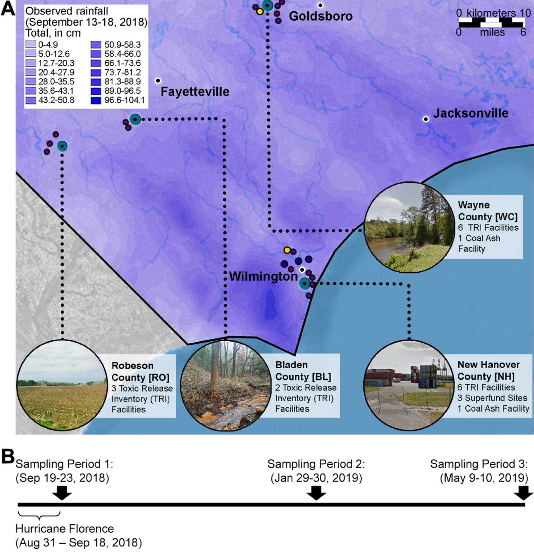
(A) Map of south-eastern North Carolina depicting sampling locations (dark blue dots) and precipitation amounts (blue shading as indicated in the color map inset) caused by Hurricane Florence in September 2018. Toxic Release Inventory facilities (purple dots), Superfund sites (dark blue dots) and coal ash facilities (yellow dots) are also indicated. Background map was from ESRI/OpenStreetMap. (B) A timeline of the Hurricane Florence and soil sample collection periods between September 2018 and May 2019. See Supplemental Table 2 for dates, locations and the number of samples collected. The GPS coordinates for sampling locations, Toxics Release Inventory and Superfund sites, and coal ash facilities are listed in Supplemental Table 14.

Sample Processing

Prior to digestion (metal analysis) or extraction (organic chemical analysis), samples were freeze-dried using model 75040 Freeze Drier 8 (Labconco, Kansas City, MO). All sample analysis results are reported based on the sample dry weight recorded after this procedure. Quality assurance procedures from NOAA National Status and Trends Program (23), US EPA Environmental Monitoring and Assessment Program-Near Coastal (24), and U.S. Fish and Wildlife Service for trace contaminant analysis (25) were followed.

Organic Compound Analysis

Freeze-dried soil samples were weighed and placed in an Accelerated Solvent Extractor (ASE, Dionex™ Model 200, Sunnyvale, CA) together with Hydromatrix™ to remove any residual water. Analyses for pesticides, PCB and PAH followed methods detailed elsewhere (26). Before extraction, experimental samples and associated quality control samples (i.e., blank, matrix spike, laboratory duplicate and standard reference material) were spiked with the appropriate surrogate standards [d₁₀-naphthalene, d₁₀-acenaphthene, d₁₀-phenanthrene, and d₁₂-chrysene, d₂₆-nC₁₂, d₄₂-nC₂₀, d₅₀-nC₂₄, d₆₂-nC₃₀, PCB 103 and 198 and 4,4-dibromooctafluorobiphenyl (DBOFB)] (27). Following extraction, samples were purified using partially deactivated silica/alumina column chromatography to eliminate interfering materials and treated with acid-washed granulated copper to eliminate potential interference from elemental sulfur.

PAH, PCB and pesticide analyses were performed by gas chromatography-mass spectrometry (GC-MS) using 6890N GC System/5975C inert Mass Selective Detector (Agilent Technologies) in selective ion mode after the addition of the appropriate internal standards (d₁₀-fluorene, d₁₂-benzo(a)pyrene, d₁₀-pyrene, and TCMX) to evaluate the efficiency of the analytical methods (27). The sample extracts were injected in the splitless mode into a 30 m×0.25 mm i.d. (0.25 μm film thickness) DB-5MS fused silica capillary column (J&W Scientific, Folsom, CA) at an initial temperature of 60°C, held for 3 min, and temperature was then programmed at 12°C min⁻¹ to 300°C with a hold of 6 min at the final temperature for PAH analytes. For PCB, the initial temperature was set at 75°C, held for 3 min, and then ramped to 150, 260, and 300°C at 0, 0, and 20°C/min, respectively, with a final hold of 1 min and a total run time of 66 min. Aliphatic hydrocarbons were analyzed by GC-flame ionization detection (FID), after the addition of d₃₈-nC₁₆ as internal standard, using a DB-5MS fused silica capillary column and an oven-temperature program starting at 40°C, held for 2 min and ramped up to 320°C at a rate of 6°C per min and a final hold of 15 min. The GC-MS and GC-FID were calibrated by injections of PCB standard mix (#48246, Sigma-Aldrich) at five concentrations (1, 10, 50, 100 and 200 ng/mL). Identification of target analytes was based on the retention time of their respective peaks (aliphatic hydrocarbons) or the respective quantitation ions and a series of confirmation ions (PAH, PCB and pesticides). Lower limit of quantitation (LLOQ, see Supplemental Tables 3 and 4 for information) was established using the lowest calibration level adjusted for the sample weight and final sample extract volume.

Metal Analysis

Freeze-dried soil samples (1g) were digested with 10 ml of a 1:1 HNO₃:DI water by heating at 95°C for 10 min. After cooling the sample to ambient temperature, 5 ml of concentrated HNO₃ was added and the sample was heated at 95°C for an additional 30 min. After cooling to ambient temperature, 3 ml of 30% H₂O₂ was added and the sample was returned to the 95°C. Additional H₂O₂ was added in 1 mL increments until effervescence is completed; the sample was then heated until the volume reached ~5 ml. The sample was filtered and brought up to a final volume of 100 ml with DI water. Instrumental analysis was performed using a NexION 300D inductively coupled plasma mass spectrometer (ICP-MS, PerkinElmer, Waltham, MA). The LLOQ was established by the measured concentration signal being 10× the standard deviation of the blank, for the analyses of trace metals the LLOQ was in the range of 0.002–50 μg/g (see Supplemental Table 5 for LLOQs for each analyte). The ICP-MS was optimized and calibrated each day of operation using one analytical blank (methylene chloride) and trace metals standard I (#C809J26, Thomas Scientific, Swedesboro, NJ) using the average of three replicate integrations. The linearity of the initial calibration was deemed sufficiently linear if r²≥0.995. The ongoing validity of the calibration was determined by the subsequent verifications performed every ten samples.

Mercury (Hg) determinations in soil samples were made after an acid-permanganate digestion of the dry-powdered samples followed by stannous chloride reduction to Hg metal and detection by cold vapor atomic absorption spectroscopy using a flow injection mercury system (Model FIMS-400, PerkinElmer). Specifically, 200 mg of each freeze-dried soil sample was digested with 4 ml of a concentrated H₂SO₄/HNO₃ (2.5:1.5 v/v) mixture by heating at 95°C for 30 min. After cooling the mixture to ambient temperature, 10 ml of DI water, 10 ml of KMnO₄ (5 g in 100 mL of DI water) solution, and 5 ml of K₂S₂O₈ (5 g in 100 mL of DI water) solution was added and the sample was heated at 95°C for 30 min. Sample was chilled to ambient temperature and 5 ml of a NaCl/H₈N₂O₆S (12 g of each in 100 mL of DI water) solution was added to reduce excess permanganate and the sample was diluted to 40 ml with DI water. The instrument was calibrated by injections of a mercury standard (#C809J26, Thomas Scientific) at five different concentrations (1, 10, 50, 100 and 200 ng/mL). The calibration was deemed sufficiently linear if r²≥0.995. Calibration verification standard and analytical blank samples were analyzed at the start and after every 10 samples and at the end of each analytical run.

Analytical Quality Control (QC)

For every batch of 20 samples or less, a procedure blank (prepared using all reagents and procedures for digestion but not containing the sample matrix), and standard reference materials (for organic compounds we used SRM 1944 - New York/New Jersey Waterway Sediment and SRM 2779 - Gulf of Mexico Crude Oil, National Institute of Standards and Technology, Gaithersburg, MD; for metals we used SRM-SAND-B, High Purity Standards, North Charleston, SC) were run to evaluate the overall accuracy and precision of the procedures used for sample preparation and analysis. Laboratory duplicates were included to estimate sample homogeneity and analytical variability. A laboratory blank spike (procedure blank fortified with appropriate trace elements and carried through digestion procedure) and a matrix spiked (fortified sample that is carried through digestion procedure and analyzed to identify any matrix dependent interferences) samples were run with each batch to identify potential digestion interferences and to evaluate the accuracy and performance of analysis. See Supplemental Tables 6–7 for QC data.

Cook’s Distance Outlier Test

Cook’s distance measure (28) was computed to determine the locations that had outlier concentrations for the individual metals. Cook’s distance D is a measure of an observations’ influence on a linear regression. Instances with a large influence may be outliers, and the measure is often computed for data sets to identify influential points that may not be good predictors for a fit of a linear model. D is calculated by removing the i_th data point from the model, recalculating the regression, and summing a scaled version of the squared estimated responses before and after the observation has been removed using formula [1]:

$${\mathit{D}}_{\mathit{i}}=\frac{{\sum }_{j=1}^n{\left({\widehat{y}}_j-{\widehat{y}}_{j\left(i\right)}\right)}^2}{p{\widehat{\sigma }}^2}$$ [1]

The ${\widehat{y}}_j$ denotes the predicted response for observation j when using the full dataset, and ${\widehat{y}}_{j\left(i\right)}$ the same fitted value when observation i has been removed, p the total number of predictors in the regression model (p=2 for our setting, including intercept), sample size n, and ${\widehat{\sigma }}^2$ the estimated error variance from the model. We deemed observation/outliers as influential with D_i>1.0. See Supplemental Table 8 for the results of this analysis.

Determining Pyrogenic Index and PAH Source Apportionment

A pyrogenic index (PI) was calculated for all samples from concentrations of the 16 EPA priority PAHs and a series of alkylated PAHs in order to determine the likely source of the PAH in each sample (29). A PI is calculated by taking the sum of concentrations of three- to six-ring PAHs and dividing it by the sum of concentrations of a series of alkylated PAHs using formula [2]:

$$\mathit{P}\mathit{I}=\frac{\sum \left(3-6\hspace{0.33em}\text{ring}\hspace{0.33em}\text{priority}\hspace{0.33em}\text{PAHs}\right)}{\sum \left(Alkylated\hspace{0.33em}PAHs\right)}$$ [2]

A value greater than one suggests that PAHs are more likely to be from a combustion source while values lower than one suggests that PAHs are more likely to be from a petroleum source. Ratios of certain PAH in environmental samples are used as indicators to determine potential sources of PAHs (30). In this study, we calculated the ratios using data on fluoranthene, pyrene, benzo(a)anthracene, chrysene, anthracene, phenanthrene, indeno(1,2,3-cd)pyrene, and benzo(g,h,i)perylene. The values for PI and selected ratios used for PAH source apportionment are listed in Supplemental Table 9.

Hazard Index and Cancer Risk Calculations

We characterized non-cancer and cancer risk values (see Supplemental Tables 10–11 for the calculated values) for each sample using U.S. EPA Regional Screening Level Soil Screening Levels (SSL) for soils (31). Non-cancer risk at each location was expressed as a hazard index (HI) and was calculated by summing the individual Hazard Quotients (HQ) for each chemical, ratios between the measured soil concentration C_k for compound k (converted to mg/kg) and the corresponding non-cancer SSL_nc,k to determine HI [3]:

$$\mathbf{HI}=\sum _{k=1}^n\frac{{\mathbf{C}}_k}{{\mathbf{SSL}}_{\text{nc},k}}$$ [3]

The calculation of HI was based on the individual PAH non-cancer SSL_nc,k corresponding to a hazard quotient of 1. Several chemicals did not have SSLs, so they were not included in the calculation.

Cancer risk for exposure to pesticides, polychlorinated biphenyls and other industrial chemicals at all locations except were calculated similarly [4], using cancer SSL_c,k corresponding to a 10⁻⁶ risk instead.

$$\mathrm{Cancer}\hspace{0.33em}\mathrm{Risk}={10}^{-6}\sum _{k=1}^n\frac{{\mathbf{C}}_k}{{\mathbf{SSL}}_{\text{c},k}}$$ [4]

For PAH cancer risks, we converted each PAH concentration to benzo[a]pyrene (BaP)-equivalents using the Toxic Equivalency Factors (TEFs) from (32), C_BaPeq,k = C_k × TEF_k, and then calculated the cancer risk [5] with the cancer SSL_c,BaP for BaP (Supplemental Table 11) (33, 34):

$$\text{PAH}\hspace{0.33em}\text{Cancer}\hspace{0.33em}\text{Risk}={10}^{-6}\sum _{k=1}^n\frac{{\mathbf{C}}_{\text{BaPeq},k}}{{\mathbf{SSL}}_{\text{c},\text{BaP}}}$$ [5]

Enrichment Factor Calculation for Metals

In order to perform a comparative analysis of presence of coal combustion-enriched metals among soil samples in this study and to the data from a previous publication (35), we calculated an enrichment factor (EF). An enrichment factor is the ratio of the concentration of each metal between a test location and a reference location and was calculated using formula [6]:

$$EFm=\frac{Ci}{Average\left(C_{BL}\right)}$$ [6]

Where EF_m is the enrichment factor for m^th metal, C_i is concentration of that metal in sample i, and C_BL is concentration of that metal in samples from Bladen county. In this study we preformed these calculations using concentrations of metals in samples downstream from the reported leaked coal ash facility (New Hanover 1 and 4). As a reference, we used an average of concentrations of each test metal from all locations in Bladen County. See Supplemental Table 12 for the product of these calculations.

Results

Soil samples were collected from a total of 28 locations in four counties in eastern North Carolina (Figure 1) in the days and months following Hurricane Florence. We note that sampling sites selected in this study were level with, or at a lower elevation than, the potential point sources of pollutants (Supplemental Figure 1); therefore, it was expected that they will be suitable for detecting pollutants that may have been re-distributed by the flooding because of Hurricane Florence. A total of 55 samples (Supplemental Tables 1–2) were collected for either organic compounds or metals. Three separate sampling campaigns were conducted over the course of 9 months (September 2018-May 2019) to establish a post-disaster “baseline” condition for comparison with contaminant levels immediately after the flooding event. Analyses were performed for a total of 92 PAH, 23 metals, 28 pesticides, 5 industrial chemicals, and 157 PCB (see raw data in Supplemental Tables 3–5).

Many of the examined substances were present in detectable levels (>LLOQ) across most samples (Figure 2). Among 16 PAH which are designated as high-priority pollutants by the EPA (36), each was found in at least 50% of the samples (Figure 2A). Fluoranthene, pyrene, benz(a)anthracene, and anthracene were found in all samples. The concentrations of PAH detected varied greatly, over several orders of magnitude. For example, concentrations of fluoranthene in soils varied from 1,487 ng/g in New Hanover county to 0.37 ng/g in Bladen county. Dibenzo(a,h)anthracene, which had the lowest detectable concentration of these PAH at 0.12 ng/g in Robeson county, was detected at 125 ng/g in New Hanover county.

Figure 2. Summary of the hazardous contaminants from various chemical classes evaluated in this study.

Left panels show percentage of soil samples which contained quantifiable amounts of (A) 16 EPA priority PAHs, (B) metals, or (C) pesticides, industrial chemicals and PCBs. Right panels show their respective ranges of concentrations as box (inter-quartile range) and whiskers (10 to 90^th percentile) plots with outliers shown as dots and median values as a vertical line. Please note that the ranges and units of measure vary between panels A-C. All raw data are available in Supplemental Tables 3-5.

Among 23 metals which were analyzed, iron, aluminum and magnesium, all naturally abundant in the Earth’s crust (37), were detected in 100% of samples (Figure 2B). Concentrations of metals also ranged widely, those naturally abundant in the Earth’s crust, such as iron (3,014–14,070 μg/g), were detected in higher concentrations. Metals which have much lower natural abundances, such as arsenic, were detected in concentrations between 1.04–4.05 μg/g. Other metals, including selenium, antimony, and barium, which are known to be found in coal ash ponds and may have potential adverse human health effects (16, 35), were found in at least 50% of samples.

Among other organic pollutants that were detected, there were 33 pesticides, industrial chemicals and PCB (Figure 2C). For example, a degradation product of the organochlorine pesticide DDT, 4,4’-DDE was detected in at least 80% of analyzed samples. The concentrations of pesticides ranged from below limits of quantitation to a maximum of 61 ng/g for endosulfan II. The median concentration of pesticides was 0.6 ng/g. Industrial chemicals were detected in 15–20% of samples and had concentrations up to a maximum of 2.9 ng/g for hexachlorobenzene. Industrial chemicals had a median concentration of 0.6 ng/g. PCB were detected in 5–35% of samples and had concentrations ranged up to a maximum of 8.7 ng/g for PCB 138/164/163.

Both spatial and temporal trends in PAH levels in soil samples are shown in Figure 3A. The heatmap shows that the distribution of PAH among locations and dates varied widely, the highest concentrations were detected in New Hanover county, mainly in location NH1 that was closest to Sutton lake. The lowest concentrations of PAH were detected in Robeson county. Next, we characterized PAH ratios in all samples to determine possible sources of contamination (Figure 3B). Based on three characteristic ratios, most of the samples contained PAH derived from coal and/or biomass combustion except for two samples, one in Wayne and one in Robeson counties, which were likely containing PAH from a petrogenic source. In addition, a pyrogenic index (PI) was calculated (38) (Figure 3C). Presence of petroleum products and/or crudes is indicated by the PI in the range of 0.01−0.05, but all of the samples in this study had PI>0.05. Petroleum product burn residue and soot samples have PI in the range of 1.5 to 2.0, while even higher PI indicate the likely pyrogenic source. We found that most samples had PI>1. In addition, we calculated PAH-based non-cancer hazard index (HI, Figure 3D) and cancer risk (Figure 3E) from exposure to residential soils. All locations had HI<<1 indicating no potential non-cancer human health risk from PAH levels detected in these samples. However, most samples in New Hanover county, and one sample each from Bladen and Wayne counties, had a PAH-based cancer risk >1×10⁻⁶ for at least one time point. Most of these samples were from the period immediately following Hurricane Florence, and NH1 location had elevated cancer risk over one order of magnitude of the regional screening level. All samples from Robeson county were <1×10⁻⁶ cancer risk threshold.

Figure 3. Data on PAH in soil samples from this study.

(A) A heatmap displays a range of concentrations of the 16 EPA priority PAH and a series of alkylated PAH used to calculate pyrogenic index at each soil sample. (B) Scatter plots showing the ratios (as depicted in the axis legends) for select PAH across all tested samples. Symbol shapes are representative of the sampling locations (see legend); symbol shading is indicative of the time when each sample was collected (black is for samples collected in September 2018, gray is for samples collected in January 2019 and white is for samples collected in May 2019). (C) The pyrogenic index (PI) was calculated for each sample as indicated in methods. The vertical dotted line indicates an upper value for PI from petroleum products or crude oil (38). Also shown are screening-level risk characterization values for non-cancer (D) and cancer (E) risks, based on EPA Soil Screening Levels. Vertical dashed lines denote screening levels of potential concern, based on a non-cancer Hazard Index=1 and a cancer risk of 10^-6. All raw data for PAH is available in Supplemental Table 11.

Regarding the analysis of metals, we first calculated distributions of each analyte in relationship to the abundance of the aluminum and iron to examine geochemical correlations used to identify metal contamination in soils (37). Then, we used Cook’s distance outlier test on the correlation analyses of each metal with aluminum (Supplemental Figure 2) or iron (Supplemental Figure 3) to determine which metals and samples may exhibit elevated concentrations. We found that the samples with outlier metal concentrations were almost exclusively from New Hanover county. Next, to determine the potential for the metal contaminants in these samples to be from the coal ash, we calculated the enrichment of metals in these New Hanover county samples as compared to Bladen county, a rural area with no known coal ash contamination (Figure 4A). As a reference of a coal ash-contaminated sediment, we also show the enrichment factors for the same metals from the recent study of Sutton coal ash pond (35), location that is upstream from the sampling sites examined herein. We found that strontium, barium, manganese, cobalt and nickel in New Hanover county samples 1 and 4 had enrichment factors similar to those in samples from Sutton coal ash pond sediment (35). Figure 4B shows a distribution of concentrations, normalized to aluminum (see Supplemental Table 13), for several metals in the samples collected in this study or those for soils from East or West North Carolina and the US (39). In the NH1 sample collected in September 2018 (marked in red on Figure 4B), concentrations of antimony, barium and strontium, metals known to be found in coal ash and ash-contaminated soil/sediments, were detected in highest amounts, as compared to other samples in this study. These concentrations were also on the high end as compared to the data for soils from North Carolina and the US (39).

Figure 4. Data on metal in soil samples from this study.

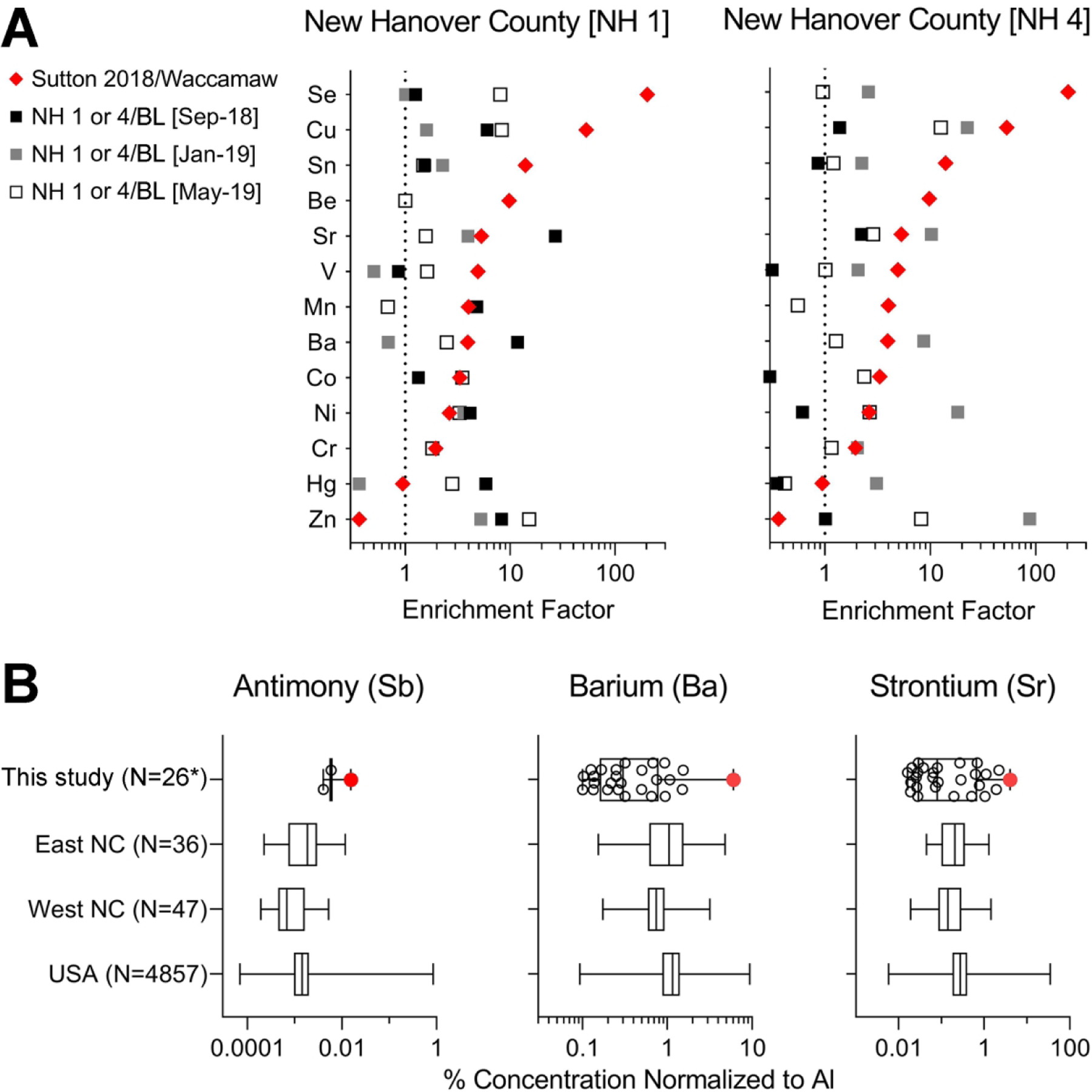
(A) Distribution and enrichment of trace metals in sediment of Sutton coal ash pond (red diamonds, from (35)) and soils (squares) from New Hanover county sites 1 and 4. Square symbol shading is indicative of the time when each sample was collected (black is for samples collected in September 2018, gray is for samples collected in January 2019 and white is for samples collected in May 2019). Sutton 2018 data was normalized to lake Waccamaw data and NH1 or 4 sample data were normalized to the average of the values for all samples from Bladen (BL) county for the corresponding time period. (B) Box and whiskers plots show the range of concentrations for antimony (Sb), barium (Ba) and strontium (Sr), normalized to aluminum, for samples from this study, or data from USGS (39) for North Carolina and the entire United States. Box is interquartile range, vertical line is the median, whiskers are min-max values. Dots in the plots for this study show individual sampling locations, the red dot indicates location NH1-September 2018. The numbers in parenthesis indicate the number of samples included into each box and whiskers plot. The asterisk indicates that one of the samples from this study (NH4-January 2019) was excluded from the metal analyses because the concentration of iron in this sample was an outlier (based on Cook’s distance) as compared to aluminum and other metals. All raw and normalized data for metals is available in Supplemental Tables 5 and 13.

We also analyzed samples from September 2018 and January 2019 for other organic compounds such as pesticides, industrial chemicals and PCB (Supplemental Table 4). We found that most of these compounds were below the limit of quantitation. Among the analytes that were quantifiable (Figure 5A), we found a number of chlorinated pesticides and PCB; most of these were found in samples from Robeson and New Hanover counties. No discernable temporal trends or spatial patterns were observed. Hazard quotients were calculated for each individual chemical and Figure 5B shows the cumulative hazard index for each sample. Even though pesticides contributed the most to hazard index in all samples, the most significant being 4,4’-DDD, all HI were <<1. Similarly, cumulative cancer risk for these chemicals (Figure 5C) was unremarkable with pesticides contributing the most to the overall cancer risk (aldrin and dieldrin with the greatest contribution).

Figure 5. Data on pesticides, industrial chemicals and PCB in soil samples from this study.

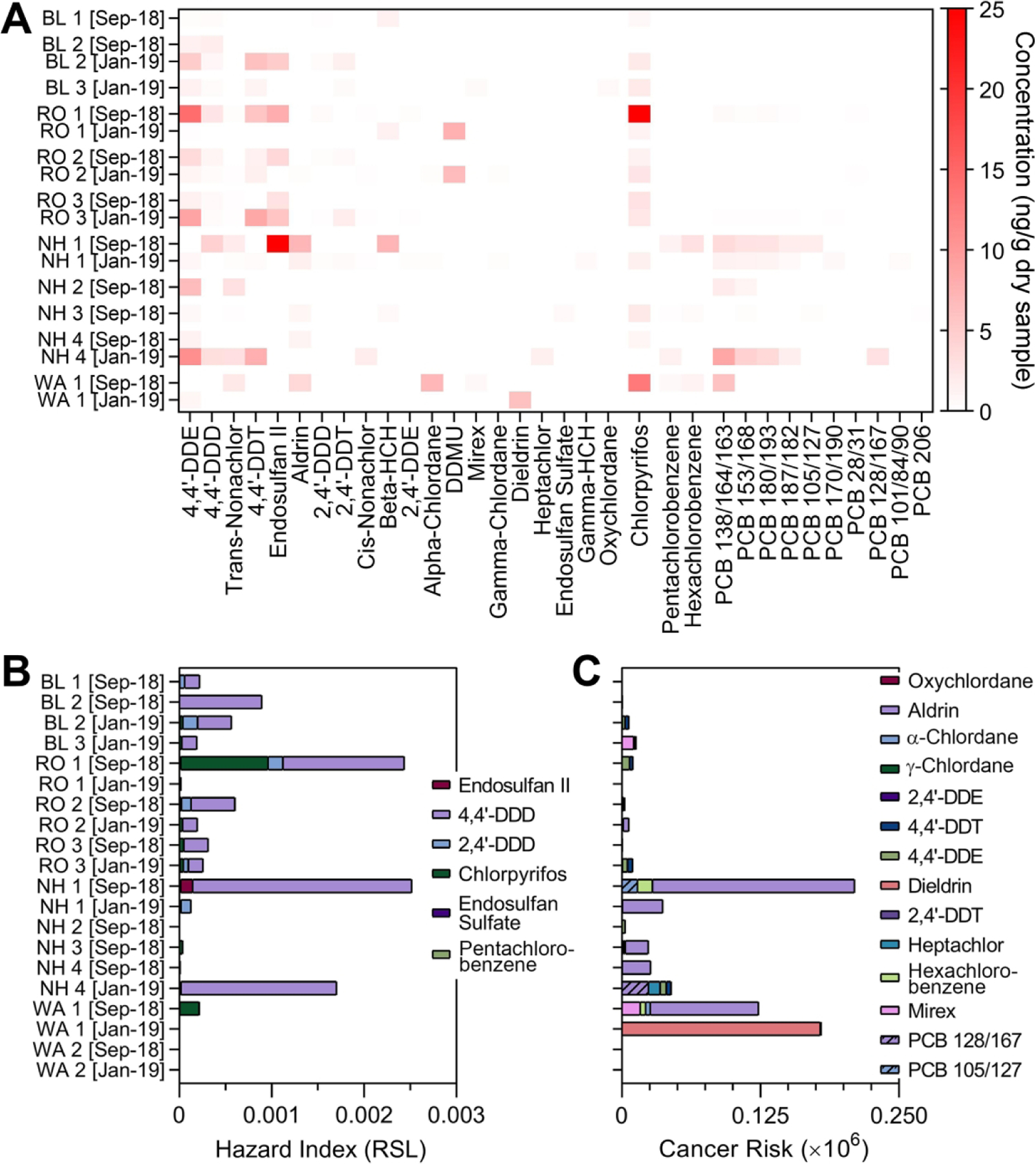
(A) A heatmap displays a range of concentrations of the detectable chemicals in each soil sample. Also shown are screening-level risk characterization values for non-cancer (B) and cancer (C) risks, based on EPA Soil Screening Levels. Stacked bar graphs contain individual compound-derived hazard quotients as indicated in the color legend next to each graph. All raw data for the chemicals displayed in this figure are available in Supplemental Table 4. Data for May 2019 were not collected because the levels of these chemicals in previous two sampling periods were unremarkable.

Discussion

Hurricane Florence was the top-10 wettest tropical cyclone on record in the United States and produced record-setting rainfall amounts for the Carolinas (40). Natural disasters in general, and flood events in particular, are known to involve mobilization of contaminants in the environment and may lead to human exposure (13). Still, the major challenges in disaster research response (DR2) and studies of the potential human exposure pathways from events like Hurricane Florence are (i) state of preparedness and ability to rapidly deploy for sample collection, (ii) informed selection of the sampling locations, and (iii) ability to make comparative analyses to the pre-disaster conditions to judge the effect of the disaster.

With respect to the degree of the overall preparedness of environmental scientists to participate in DR2, a number of scientific questions about the environmental health impacts of disasters and the effectiveness of response and recovery strategies are now considered through major government-academia coordination efforts (41, 42). Both national, regional and local capacity in DR2 is now established for researchers through training in field study design, environmental sample collection, and safety procedures associated with deployments into the areas where restrictions on public access are just being removed and dangers may still exist (43). Indeed, such prior training and availability of sampling supplies to rapidly deploy to North Carolina allowed our research group to conduct environmental sampling immediately after the rain subsided. These samples represent the most direct evidence of the environmental conditions in the areas impacted by flooding.

Selection of sampling locations in a large area effected by the Hurricane Florence-associated flooding was based on input from local non-governmental organizations and media reports (18–20). Specifically, it was determined that coal ash was one of the concerns from the Hurricane Florence floodwaters, because it is a hazardous waste by-product of coal-fired electric power plants. Coal ash contains high levels of metals, PAH and other hazardous substances (17, 44, 45). Indeed, concerns over the release of these hazardous substances with coal ash from a number of storage sites flooded by the Hurricane Florence-associated precipitation were documented in North Carolina (46). Other potential environmental chemical exposure vectors included flooding of the farms, transportation infrastructure, and municipal water treatment facilities. To account for the vast area impacted by the flooding and to select representative locations for various types of contaminants (Figure 1), we chose areas with a known coal ash spill (New Hanover county), with a coal ash facility that did not leak or flood (Wayne county), as well as agricultural use areas with some small-scale manufacturing facilities and previous reports to the toxic release inventory (Robeson and Bladen counties). Overall, none of these areas had information on the broad range of environmental contaminants; therefore, sampling after the disaster was deemed to be the most sensible strategy to determine whether the event resulted in toxic releases of concern to human health.

The most notable finding of our study is the observation that except for the areas impacted by the known coal ash spill from Sutton lake in New Hanover county, few other sampled locations demonstrated evidence for re-distribution of the hazardous contaminants in the environment because of Hurricane Florence. These data are important for two reasons. First, because they provide actionable information to alleviate community concerns about flood waters potentially carrying hazardous substances from the sites of storage to the areas where exposures to the general population may occur. Indeed, not only we reported the levels of PAH, metals and other chemicals, we also showed that based on these data, both non-cancer hazard and cancer risks from exposures through residential soils in most of the areas tested were negligible. Second, these data provide important reference information for comparison in future studies. Eastern North Carolina is prone to flooding associated with tropical cyclones (e.g., hurricanes Fran in 1996 and Matthew in 2016) and it is likely that an event similar to the Hurricane Florence may occur soon. Comparative analysis of pre- and post-disaster exposure pathways is among the biggest challenges in DR2 (26, 47).

A number of previous reports examined spatial and temporal trends in trace metal redistribution in the environment following major flooding events of coal ash contaminated areas. For example, an 18-month investigation of the Tennessee Valley Authority (TVA) coal ash spill found that concentrations of arsenic, a leachable coal ash contaminant, increased over time at sites downstream from the spill (16). A study monitoring unlined coal ash ponds in Southeastern United States has found coal ash residuals in nearby water sources even in absence of any major flooding events (48). However, studies following Hurricane Katrina (49, 50) found insignificant spatial and temporal changes for both PAH and trace metal concentrations in sediments from the Mississippi Gulf Coast over a year-long study period. In our study, evidence of metal and PAH contaminant re-distribution associated with Hurricane Florence flooding was found at the location that was closest to a documented coal ash spill (35). Together, these studies suggest site-specific spatial and temporal trends and difficulty of extrapolating without detailed sampling and exposure assessment.

In addition, the “positive” findings of our study also constitute a number of public health-informative outcomes. Specifically, we showed that the coal ash-associated PAH and metals were found downstream from the pond breach site for the Sutton lake facility. One previous study showed that levels of coal ash-associated metals in the Cape Fear river close to Sutton lake were lower than those in the coal ash pond sediment, but still elevated (35). Indeed, we provide evidence that coal ash spill may have reached further downstream (Figure 6A) because we observed temporal and spatial trends in strontium, barium and antimony, strongest at NH1 site closest to Sutton lake, indicative of the higher concentrations in September 2018, immediately after the spill. The PAH data at this location, however, showed elevated levels at all three sampling time periods and it is difficult to conclude that at this sampling site, which is in the industrial area, that the levels of PAH are from the coal ash spill as opposed to representative of the historical contamination because of other pyrogenic sources. Still, lack of finding of the elevated levels of both metals and PAH at the areas around several capped coal ash ponds in Wayne county (Figure 6B) indicate that that area did not suffer from an unmonitored coal ash spill and that the primary areas of concern, as indicated by the high cancer risk from PAH, was in New Hanover county. Overall, because only a total of three time points was sampled in our study, it is challenging to draw strong conclusions regarding temporal trends or determine whether there may be a causal relationship between flooding and the presence of contaminants. Thus, the need for more comprehensive baseline monitoring remains key to understanding the impact of natural disasters on release and/or redistribution of contaminants.

Figure 6. Map of two sampled coal ash pond locations and surrounding areas in south-eastern North Carolina.

Sampling locations (blue inverted water drops) are indicated with the location ID (see Supplemental Table 2 for detailed sample location information). (A) Locations in New Hanover county are shown. Sutton lake coal ash pond is outlined in red. (B) Locations in Wayne county are shown. Retired coal ash ponds near Quaker Neck lake are outlined in red. Background maps were from ESRI/OpenStreetMap.

Overall, this study presents a comprehensive new dataset that includes both temporal and spatial data on a broad range of hazardous substances of human health relevance. We present evidence for the lack of human health concern in most of the studies areas in eastern North Carolina that were impacted by extensive flooding during Hurricane Florence. At the same time, we show that the reported coal ash spill in New Hanover county was likely associated with release of a number of hazardous contaminants that were detected at elevated levels >10 kilometers downstream. This and previous coal ash spills that were largely unmonitored have resulted in mobilization of a number of soluble hazardous substances through the floodwaters. Because of the possible widespread transport of contaminated waters and elevated levels of hazardous substances in the soils, additional detailed and longitudinal exposure assessment studies are needed in the areas closest to the sites of unmonitored coal ash spills, especially those that may be affected by natural disasters.

References

- 1.Plumlee GS, Morman GP, Meeker TM, Hoefen PL, Hageman RE, Wolf RE. 11.7 - The Environmental and Medical Geochemistry of Potentially Hazardous Materials Produced by Disasters. Treatise on Geochemistry 2014;11:257–304. [Google Scholar]
- 2.Rieble DD, Hass CN, Pardue J, Walsh W. Toxic and contaminant concerns generated by hurricane Katrina. J Environ Engin 2006;36(1):5–13. [Google Scholar]
- 3.Diaz JH. The public health impact of hurricanes and major flooding. J La State Med Soc 2004;156(3):145–50. [PubMed] [Google Scholar]
- 4.Ahern M, Kovats RS, Wilkinson P, Few R, Matthies F. Global health impacts of floods: epidemiologic evidence. Epidemiol Rev 2005;27:36–46. [DOI] [PubMed] [Google Scholar]
- 5.Joyce S. The dead zones: oxygen-starved coastal waters. Environ Health Perspect 2000;108(3):A120–5. [DOI] [PMC free article] [PubMed] [Google Scholar]
- 6.Euripidou E, Murray V. Public health impacts of floods and chemical contamination. J Public Health (Oxf) 2004;26(4):376–83. [DOI] [PubMed] [Google Scholar]
- 7.Cruz AM, Steinberg LJ, Luna R. Identifying hurricane-induced hazardous material release scenarios in a petroleum refinery. Nat Hazards Rev 2001;2(4):203–10. [Google Scholar]
- 8.Krausmann E, Mushtaq F. A qualitative Natech damage scale for the impact of floods on selected industrial facilities. Nat Hazards 2008;46(2):179–97. [Google Scholar]
- 9.Mandigo AC, DiScenza DJ, Keimowitz AR, Fitzgerald N. Chemical contamination of soils in the New York City area following Hurricane Sandy. Environ Geochem Health 2016;38(5):1115–24. [DOI] [PubMed] [Google Scholar]
- 10.Woodruff JD, Irish JL, Camargo SJ. Coastal flooding by tropical cyclones and sea-level rise. Nature 2013;504(7478):44–52. [DOI] [PubMed] [Google Scholar]
- 11.Peduzzi P, Chatenoux B, Dao H, De Bono A, Herold C, Kossin J, et al. Global trends in tropical cyclone risk. Nature Climate Change 2012;2:289. [Google Scholar]
- 12.Knutson TR, McBride JL, Chan J, Emanuel K, Holland G, Landsea C, et al. Tropical cyclones and climate change. Nature Geoscience 2010;3:157. [Google Scholar]
- 13.Knap AH, Rusyn I. Environmental exposures due to natural disasters. Rev Environ Health 2016;31(1):89–92. [DOI] [PMC free article] [PubMed] [Google Scholar]
- 14.Winsor M. Timeline of Florence as slow-moving, deadly storm batters Carolinas. ABC News 2018. [Google Scholar]
- 15.Coyte RM, McKinley KL, Jiang S, Karr J, Dwyer GS, Keyworth AJ, et al. Occurrence and distribution of hexavalent chromium in groundwater from North Carolina, USA. Sci Total Environ 2020;711:135135. [DOI] [PubMed] [Google Scholar]
- 16.Ruhl L, Vengosh A, Dwyer GS, Hsu-Kim H, Deonarine A. Environmental impacts of the coal ash spill in Kingston, Tennessee: an 18-month survey. Environmental science & technology 2010;44(24):9272–8. [DOI] [PubMed] [Google Scholar]
- 17.U.S. EPA. Coal Ash Basics Washington, DC: U.S. Environmental Protection Agency; 2020[cited 2020 October 12]; Available from: https://www.epa.gov/coalash/coal-ash-basics. [Google Scholar]
- 18.Dewitt D. Researcher: Sutton Lake Site Of Numerous Coal Ash Spills. North Carolina Public Radio 2019. [Google Scholar]
- 19.Ouzts E. Critics: North Carolina officials ‘failing’ after Florence coal ash spills. Energy News Network, [Internet].2018October12, 2020. Available from: https://energynews.us/2018/10/16/southeast/critics-north-carolina-officials-failing-after-florence-coal-ash-spills/. [Google Scholar]
- 20.Biesecker M, Kastanis A. Hurricane Florence breaches manure lagoon, coal ash pit in North Carolina2018 Available from: https://www.pbs.org/newshour/nation/hurricane-florence-breaches-manure-lagoon-coal-ash-pit-in-north-carolina. [Google Scholar]
- 21.National Hurricane Center. Tropical Cyclone Report: Hurricane Florence Miami, FL: 2019Contract No.: AL062018. [Google Scholar]
- 22.U.S. EPA. Soil Sampling Operating Procedure In: U.S. Environmental Protection Agency, editor. Athens, GA: U.S. EPA; 2007. [Google Scholar]
- 23.Cantillo AY, Lauenstein GG. Performance-Based Quality Assurance—The NOAA National Status and Trends Program Experience In: Administration NOaA, editor. Silver Spring, MD1998. [Google Scholar]
- 24.U.S. EPA. National Coastal Condition Assessment Quality Assurance Project Plan In: United States Environmental Protection Agency, editor. Washington, DC2010. [Google Scholar]
- 25.Silva MH, Kwok A. Open Access ToxCast/Tox21, Toxicological Priority Index (ToxPi) and Integrated Chemical Environment (ICE) Models Rank and Predict Acute Pesticide Toxicity: A Case Study. Int J Toxicol Envr Health 2020;5(1):102–25. [Google Scholar]
- 26.Bera G, Camargo K, Sericano JL, Liu Y, Sweet ST, Horney J, et al. Baseline data for distribution of contaminants by natural disasters: results from a residential Houston neighborhood during Hurricane Harvey flooding. Heliyon 2019;5(11):e02860. [DOI] [PMC free article] [PubMed] [Google Scholar]
- 27.El-Kady AA, Wade TL, Sweet ST, Sericano JL. Distribution and residue profile of organochlorine pesticides and polychlorinated biphenyls in sediment and fish of Lake Manzala, Egypt. Environ Sci Pollut Res Int 2017;24(11):10301–12. [DOI] [PubMed] [Google Scholar]
- 28.Cook RD. Detection of Influential Observations in Linear Regression. Technometrics 1977;19(1):15–8. [Google Scholar]
- 29.Wang Z, Yang C, Parrott JL, Frank RA, Yang Z, Brown CE, et al. Forensic source differentiation of petrogenic, pyrogenic, and biogenic hydrocarbons in Canadian oil sands environmental samples. J Hazard Mater 2014;271:166–77. [DOI] [PubMed] [Google Scholar]
- 30.Lu J, Zhang C, Wu J, Lin YC, Zhang YX, Yu XB, et al. Pollution, sources, and ecological-health risks of polycyclic aromatic hydrocarbons in coastal waters along coastline of China. Hum Ecol Risk Assess 2020;26(4):968–85. [Google Scholar]
- 31.U.S. EPA. Regional Screening Levels RSLS Generic Tables Washington, DC: U.S. Environmental Protection Agency; 2020[July 01, 2020]; Available from: https://www.epa.gov/risk/regional-screening-levels-rsls-generic-tables. [Google Scholar]
- 32.Nisbet IC, LaGoy PK. Toxic equivalency factors (TEFs) for polycyclic aromatic hydrocarbons (PAHs). Regulatory toxicology and pharmacology : RTP 1992;16(3):290–300. [DOI] [PubMed] [Google Scholar]
- 33.U.S. EPA. Development of a Relative Potency Factor (Rpf) Approach for Polycyclic Aromatic Hydrocarbon (PAH) Mixtures (External Review Draft) Washington, DC: U.S. Environmental Protection Agency; 2010. [Google Scholar]
- 34.U.S. EPA. Provisional Guidance for Quantitative Risk Assessment of Polycyclic Aromatic Hydrocarbons (PAH) Washington, DC: U.S. Environmental Protection Agency, Office of Research and Development, Office of Health and Environmental Assessment; 1993. [Google Scholar]
- 35.Vengosh A, Cowan EA, Coyte RM, Kondash AJ, Wang Z, Brandt JE, et al. Evidence for unmonitored coal ash spills in Sutton Lake, North Carolina: Implications for contamination of lake ecosystems. Sci Total Environ 2019;686:1090–103. [DOI] [PubMed] [Google Scholar]
- 36.IARC. Some Non-heterocyclic Polycyclic Aromatic Hydrocarbons and Some Related Exposures Cancer IAfRo, editor. Lyon, France: WHO; 2010. [PMC free article] [PubMed] [Google Scholar]
- 37.Myers J, Thorbjornsen K. Identifying metals contamination in soil: A geochemical approach. Soil Sediment Contam 2004;13(1):1–16. [Google Scholar]
- 38.Wang ZD, Fingas M, Shu YY, Sigouin L, Landriault M, Lambert P, et al. Quantitative characterization of PAHs in burn residue and soot samples and differentiation of pyrogenic PAHs from petrogenic PAHs - The 1994 Mobile Burn Study. Environmental science & technology 1999;33(18):3100–9. [Google Scholar]
- 39.USGS. Geochemical and Mineralogical Data for Soils of the Conterminous United States In: U.S. Department of the Interior, editor. Reston, VA: U.S. Geological Survey; 2013. [Google Scholar]
- 40.National Weather Service. Historical Hurricane Florence, September 12 – 15, 2018 2018[cited 2018 December 15]; Available from: https://www.weather.gov/mhx/Florence2018.
- 41.Errett NA, Haynes EN, Wyland N, Everhart A, Pendergrast C, Parker EA. Assessing the national capacity for disaster research response (DR2) within the NIEHS Environmental Health Sciences Core Centers. Environ Health 2019;18(1):61. [DOI] [PMC free article] [PubMed] [Google Scholar]
- 42.Horney JA, Rios J, Cantu A, Ramsey S, Montemayor L, Raun L, et al. Improving Hurricane Harvey Disaster Research Response Through Academic-Practice Partnerships. Am J Public Health 2019;109(9):1198–201. [DOI] [PMC free article] [PubMed] [Google Scholar]
- 43.Amolegbe S. Texas workshop prepares trainees for disaster research. NIEHS Environmental Factor, [Internet] 2019April01, 2020. Available from: https://factor.niehs.nih.gov/2019/3/science-highlights/disaster_research/index.htm. [Google Scholar]
- 44.Schwartz GE, Hower JC, Phillips AL, Rivera N, Vengosh A, Hsu-Kim H. Ranking Coal Ash Materials for Their Potential to Leach Arsenic and Selenium: Relative Importance of Ash Chemistry and Site Biogeochemistry. Environ Eng Sci 2018;35(7):728–38. [DOI] [PMC free article] [PubMed] [Google Scholar]
- 45.Srivastava VK, Srivastava PK, Misra UK. Polycyclic aromatic hydrocarbons of coal fly ash: analysis by gas-liquid chromatography using nematic liquid crystals. J Toxicol Environ Health 1985;15(2):333–7. [DOI] [PubMed] [Google Scholar]
- 46.Kravchenko J, Lyerly HK. The Impact of Coal-Powered Electrical Plants and Coal Ash Impoundments on the Health of Residential Communities. N C Med J 2018;79(5):289–300. [DOI] [PubMed] [Google Scholar]
- 47.Horney JA, Casillas GA, Baker E, Stone KW, Kirsch KR, Camargo K, et al. Comparing residential contamination in a Houston environmental justice neighborhood before and after Hurricane Harvey. PloS one 2018;13(2):e0192660. [DOI] [PMC free article] [PubMed] [Google Scholar]
- 48.Harkness JS, Sulkin B, Vengosh A. Evidence for Coal Ash Ponds Leaking in the Southeastern United States. Environmental science & technology 2016;50(12):6583–92. [DOI] [PubMed] [Google Scholar]
- 49.Weston J, Warren C, Chaudhary A, Emerson B, Argote K, Khan S, et al. Use of bioassays and sediment polycyclic aromatic hydrocarbon concentrations to assess toxicity at coastal sites impacted by Hurricane Katrina. Environ Toxicol Chem 2010;29(7):1409–18. [DOI] [PubMed] [Google Scholar]
- 50.Warren C, Duzgoren-Aydin NS, Weston J, Willett KL. Trace element concentrations in surface estuarine and marine sediments along the Mississippi Gulf Coast following Hurricane Katrina. Environ Monit Assess 2012;184(2):1107–19. [DOI] [PubMed] [Google Scholar]
Associated Data
This section collects any data citations, data availability statements, or supplementary materials included in this article.