Dynamic and reversible remapping of network representations in an unchanging environment

Isabel I C Low; Alex H Williams; Malcolm G Campbell; Scott W Linderman; Lisa M Giocomo

doi:10.1016/j.neuron.2021.07.005

. Author manuscript; available in PMC: 2022 Sep 15.

Published in final edited form as: Neuron. 2021 Aug 6;109(18):2967–2980.e11. doi: 10.1016/j.neuron.2021.07.005

Dynamic and reversible remapping of network representations in an unchanging environment

Isabel I C Low ^1,^2,^*, Alex H Williams ^2,³, Malcolm G Campbell ^1,⁴, Scott W Linderman ^2,³, Lisa M Giocomo ^1,^2,^5,^*

PMCID: PMC8448985 NIHMSID: NIHMS1725525 PMID: 34363753

Summary:

Neurons in the medial entorhinal cortex alter their firing properties in response to environmental changes. This flexibility in neural coding is hypothesized to support navigation and memory by dividing sensory experience into unique episodes. However, it is unknown how the entorhinal circuit as a whole transitions between different representations when sensory information is not delineated into discrete contexts. Here, we describe rapid and reversible transitions between multiple spatial maps of an unchanging task and environment. These remapping events were synchronized across hundreds of neurons, differentially impacted navigational cell types, and correlated with changes in running speed. Despite widespread changes in spatial coding, remapping comprised a translation along a single dimension in population-level activity space, enabling simple decoding strategies. These findings provoke a reconsideration of how medial entorhinal cortex dynamically represents space and suggest a remarkable capacity for cortical circuits to rapidly and substantially reorganize their neural representations.

Keywords: medial entorhinal cortex, dynamic coding, behavioral state, population coding, attractor manifolds

eTOC Blurb:

Low et al. record from hundreds of neurons in entorhinal cortex and reveal transitions between distinct neural maps of space in an unchanging task and environment. These transitions are reversible, synchronized across neurons, and correlated with running speed. Alignment of the two activity manifolds enables reliable position decoding across maps.

Graphical Abstract

graphic file with name nihms-1725525-f0009.jpg

Introduction

As an animal engages in complex behaviors, it must dynamically integrate external sensory features with internal behavioral state changes. Arousal (Hulse et al., 2017; Salay et al., 2018; Vinck et al., 2015), satiety (Jennings et al., 2019), attention (Kentros et al., 2004), and running speed (Bennett et al., 2013; Hardcastle et al., 2017; Hulse et al., 2017; Niell and Stryker, 2010; Vinck et al., 2015) can all impact cortical processing and influence how an animal interacts with its surroundings (Calhoun et al., 2019; Salay et al., 2018). As an animal navigates the world, encountering a continuous stream of sensory features while experiencing behavioral state changes, navigational centers in the brain may integrate these external and internal factors to encode unique episodes or contexts. The extent to which these navigational centers incorporate changes in an animal’s internal behavioral state, as opposed to reflecting the external sensory features in the world, remains incompletely understood.

One key navigational center is the medial entorhinal cortex (MEC), which is hypothesized to support navigation and memory through neurons that encode the animal’s position and orientation relative to sensory features such as environmental boundaries and objects (Diehl et al., 2017; Gil et al., 2018; Hafting et al., 2005; Høydal et al., 2019; Sargolini et al., 2006; Solstad et al., 2008). When environmental features change, MEC position and orientation cells can “remap” through changes in firing rate and rotations or shifts in firing field locations (Barry et al., 2007; Diehl et al., 2017; Fyhn et al., 2007; Keene et al., 2016; Krupic et al., 2015; Marozzi et al., 2015; Munn et al., 2020; Solstad et al., 2008). This flexibility in MEC neural coding is hypothesized to be an integral part of navigational and memory processes. It may also interface with a similar phenomenon in the hippocampus (Fyhn et al., 2007), a neural substrate involved in memory formation, where neurons also remap in response to changes in sensory features or task context (Bostock et al., 1991; Frank et al., 2000; Jezek et al., 2011; Markus et al., 1995; Moita et al., 2004; Muller and Kubie, 1987; Wood et al., 2000). Recent work in the hippocampus has revealed remapping in response to other latent factors, which may include changes in an animal’s behavioral state (Keinath et al., 2020; Sheintuch et al., 2020; Ziv et al., 2013), suggesting that MEC may be responsive to these factors as well. Consistent with this possibility, changes in task demands can evoke MEC remapping (Boccara et al., 2019; Butler et al., 2019). However, studies have yet to identify the specific impact of latent factors such as behavioral state on MEC remapping. Further, it is not yet known what MEC remapping dynamics might look like when environmental features or task demands are not delineated into distinct episodes.

Until recently, technological constraints limited most studies to small numbers of simultaneously recorded MEC neurons. As a result, previous studies of flexibility in MEC neural coding often focused on how the firing fields of single functionally-defined neurons (e.g. grid, border, or head direction cells) responded to changing environmental features. However, not all MEC neurons fall into discrete functional classes (Hardcastle et al., 2017; Hinman et al., 2016) and many MEC coding properties are proposed to emerge at the population level (Burak and Fiete, 2009; Couey et al., 2013; Fuhs and Touretzky, 2006; McNaughton et al., 2006; Ocko et al., 2018; Pastoll et al., 2013). These features of MEC coding raise the question of how the the MEC circuit as a whole transitions between contextual representations.

Here, we investigated how large populations of MEC neurons transition between spatial representations in an invariant environmental context. Using silicon probes, we simultaneously recorded from hundreds of MEC neurons while mice navigated a virtual reality (VR) environment. We found that remapping events occurred synchronously across the MEC population—recruiting a large swath of cells with heterogeneous coding properties—without any change in environmental features or task demands. Further, we demonstrated that each map corresponded to a distinct activity manifold. Running speed correlated with transitions between these manifolds and the manifolds for different maps were geometrically aligned, which enabled consistent position decoding in spite of remapping. Altogether our findings demonstrate that a single population of neurons can preserve unchanging information (e.g. fixed environmental features), while also encoding changes in internal context, demonstrating a remarkable capacity for both reliability and flexibility in MEC navigational coding.

Results

Spatial representations remap in an invariant VR environment

Head-fixed mice foraged for water rewards along an infinite VR track with landmark cues that repeated every 400 cm (Campbell et al., 2020)(Figure 1A, B; Figure S1). 11 mice navigated a cue rich track (5 landmarks, Figure 1B, top)(n = 43 sessions, i.e., cue rich sessions), 6 mice navigated a cue poor track (2 landmarks, Figure 1B, bottom)(n = 11 sessions, i.e., cue poor sessions), and 5 mice navigated alternating blocks of cue rich and cue poor trials within each each session (n = 13 sessions, i.e., double-track sessions). Mice could lick for water in a visually marked reward zone, which appeared at random locations along the track (Figure S1). In reward zones, mice slowed (difference in running speed, 11.7 ± 1.2 cm/s; p = 3.1×10⁻¹¹) and licked for water (difference in lick number 8.0 ± 0.2; p < 1×10⁻¹¹), demonstrating familiarity with the task (Figure 1C–F).

To record neural activity during behavior, we acutely inserted Neuropixels silicon probes (Jun et al., 2017) into MEC for up to six recording sessions per mouse (up to three sessions per hemisphere). Each session was associated with a unique probe insertion and sessions from the same hemisphere were recorded in distinct parts of MEC (Figure S1; STAR Methods). Thus we recorded simultaneously from hundreds of neurons across a large portion of the MEC dorsal to ventral axis in individual mice (n = 10,410 cells)(Figure 1G, H; Figure S1). To quantify spatial coding stability across co-recorded neurons, we estimated each neuron’s position-aligned firing rate on each trial and computed the correlation between all spatial representations for each pair of trials (STAR Methods). Network-wide position coding was typically stable across neighboring trials (moving average correlation, 5 nearest trials: 0.441 ± 0.009)(Figure 1I, J; STAR Methods). In some cases population-wide neural representations appeared untethered from landmarks for part or all of the session (interquartile range min to max: 0.034 to 0.394)(Figures S1, S2).

To characterize the stability of population-wide spatial coding across all trials for each session, we collected the spatial correlations for all trial pairs into a trial-by-trial similarity matrix of network-wide spatial representations (Figure 2B–F right; Figure S2). In many recording sessions, we observed clear changes in these similarity matrices and in the spatial firing patterns of single neurons distributed across MEC (i.e., remapping events) (Figure 2B–F; Figure S2). These remapping events occurred without any change to environmental sensory cues or task demands. Importantly, remapping events did not reflect recording probe movement (Figures S1, S3). MEC cells often switched abruptly between stable spatial representations (i.e., maps)(Figure 2A), with cells returning repeatedly to one of several distinct maps within a single session, resulting in a checkerboard pattern of trial-by-trial similarity (Figure 2B–F; Figures S1, S2). In other sessions, spatial representations underwent a single transition between stable maps or transitioned between spatially stable and unstable coding regimes (Figure 2B, F; Figure S2). While the frequency and stability of remapping was thus heterogeneous across mice and sessions, in all cases remap events appeared to recruit co-recorded neurons all along the dorsal to ventral MEC axis (Figure 2B–F, right; Figures S1, S2).

Figure 2: — (A) Rasters (top) and tuning curves (bottom) for four example cells (40 example trials) from one session (black lines, average firing rate; shading, SEM; same as Fig. 1J). (B) Full rasters (left) and network-wide trial-by-trial similarity matrix (right) from the same example session (arrowheads, transitions in spatial coding; colors alternate light/dark for discernibility; colorbar, trial-by-trial spatial correlation)(n = 142 cells). (C, D) As in B, but for a different example cue poor (C; n = 227 cells) and cue rich (D; n = 139 cells) session. (E, F) As in (B-D), but for one double-track session split into cue poor (E) and cue rich (F) trial blocks (dashed lines indicate breaks between blocks; n = 55 cells). (B-F) Pink arrowheads indicate cue rich track; green, cue poor. (See also Figure S2, S3.)

Data-driven detection of network-wide remapping

To characterize neural remapping not related to changing visual cues, we focused our main analysis on sessions from mice who only experienced one of the two tracks (single-track sessions; n = 54 sessions in 17 mice). Double-track sessions recapitulated all major single-track findings, indicating that the general properties of network-wide remapping were consistent across different VR tasks (Figure S4). To group trials with similar network-wide spatial activity, we applied k-means clustering to each session (Figure 3A). The k-means model assigns a single cluster label to each trial and these cluster labels often visibly matched the checkerboard pattern in trial-by-trial similarity matrices (Figure 3B; Figures S2, S5). Despite making the strict assumption that each trial belongs to a single spatial map, a 2-cluster k-means model consistently approached the performance of a less constrained uncentered PCA model, which allows each trial to contain a blend of multiple spatial maps (Figure 3C). These results suggest that remapping events were well-approximated by discrete transitions between spatial maps.

Figure 3: — (A) Schematized k-means clustering strategy: raw spikes (top) are converted to normalized firing rate (center), k-means gives a low-dimensional estimate of the neural activity (bottom). (B) Trial-by-trial similarity (top, as in Figure 2B–F), distance score for population-wide neural activity by trial (middle; a score of 1 indicates that population activity is in the map 1 k-means cluster centroid; score = −1, map 2 centroid), and single neuron distance to k-means cluster centroid across trials, sorted by depth (bottom; colorbar, distance to cluster: gray, midway between maps; black, at or beyond map 1 centroid; white, map 2) for an example session (mouse 1c, session 0430_1, n = 227 cells). (C) 2-factor k-means versus PCA performance (uncentered R²) for all single-track sessions (left). Model performance for uncentered PCA (indigo), k-means (gold), and k-means on shuffled data (gray) for an example session (right)(mouse 1c, session 0501_1, n = 122 cells). (D) Selection criteria for 2-map sessions (gold shading; performance gap with PCA < 70% relative to shuffle, $R_{kmeans}^{2} > 0.63$ ). (E) Average trial-to-trial spatial similarity for trials from the same map versus across maps for all 2-map sessions (mean change in correlation ± SEM: −32.43 ± 2.57%; Wilcoxon signed-rank test, p = 3.79×10⁻⁶)(green, cue poor sessions; pink, cue rich). (F) Percent of all cells that were consistent remappers by location in MEC (4,108/4,984 cells). (C, D) n = 54 sessions, 17 mice; (E, F) n = 4,984 cells, 28 sessions, 13 mice. (See also Figure S2, S5.)

Using the relative performance of k-means to PCA, we identified 28 out of 54 single-track sessions that were adequately fit by a 2-cluster k-means model (Figure 3D, n = 23 cue rich sessions, 5 cue poor sessions; 4,984 cells; 13 mice). In many of these sessions, neural activity repeatedly returned to the same set of maps (13/28 sessions exhibited three or more remap events)(Figure S3). Trials within a given map were more similar to each other than to trials from the other map (p = 3.79×10⁻⁶)(Figure 3E). We focused subsequent analysis on these 28 “2-map sessions,” as they were the simplest and most common case. The remaining 26 sessions showed heterogeneous remapping that was not well-captured by this two factor model (Figures 2, S1, S2, S5).

How do these network-wide events recruit single neurons? In 2-map sessions, the majority of cells throughout MEC (82.4%) changed their firing properties in precise agreement with population-derived remapping events (i.e., consistent remappers, average distance to cluster centroid < 1)(Figure 3B bottom, Figure 3F)(STAR Methods). There was some regional variability in the proportion of these consistent remappers, but they always comprised the bulk of the population (Figure 3F). Thus, most MEC neurons remapped abruptly and synchronously.

Entorhinal neurons reversibly and heterogeneously remap

We next asked how remapping influences the coding properties of single MEC neurons. In 2-map sessions, many single neurons exhibited distinct spiking patterns and spatial tuning curves within each k-means identified map (Figure 4A; see Figure S5 for >2-map sessions). To quantify these tuning changes, we calculated the change in peak firing rate (i.e., rate remapping) and the spatial dissimilarity (i.e., global remapping) across the two maps for each cell (Knierim et al., 1998; Muller and Kubie, 1987; O’Keefe and Conway, 1978)(STAR Methods). Across all cells (spatial and non-spatial), we observed diverse remapping responses, with no obvious clustering in type of remapping (Figure 4B, C). Many cells showed some rate remapping (median absolute change in peak firing rate: 1.28-fold), but largely retained their spatial tuning across maps (median spatial dissimilarity: 0.031)(Figure 4A–C). Nevertheless, the dissimilarity distribution was heavy-tailed (Figure 4B), indicating a subpopulation of cells with large changes in spatial tuning across maps (5% of cells had dissimilarity > 0.223)(e.g. Figure 4A, C, cool colors).

Cells also exhibited changes in spatial information across the two maps (e.g. Figure 4D), resulting in many cells (13 ± 1%) that were significantly spatial in one map, but not the other (p < 0.05)(Figure 4E). Cells with high spatial information in at least one map were likely to remap in coordination with the rest of the population (1,449 out of 1,545 spatial cells)(Figure 4F). Thus remapping reflected changes in the spatial coding properties of MEC neurons and recruited most spatially informative cells.

Navigationally relevant cell types differentially remap

MEC contains functional cell types that exhibit distinct spatial coding statistics (e.g. grid, border, object vector, and head direction cells)(Hafting et al., 2005; Høydal et al., 2019; Kropff et al., 2015; Sargolini et al., 2006; Savelli et al., 2008; Solstad et al., 2008), raising the question of how remapping recruits these cell types. To investigate this question, we leveraged a previous finding that grid cells are responsive to mismatches between visual and motor feedback in 1D VR, while border cells remain stable (Campbell et al., 2018). In a subset of 2-map sessions (n = 9 cue rich sessions), we appended 5 trials in which the mouse had to run twice as far to traverse the same visual landscape (i.e., gain mismatch)(Figure 5A). We classified spatially stable cells that were highly responsive to gain mismatch as putative grid cells (224 out of 1,379 cells) and those that were unaffected by gain mismatch as putative border cells (152 cells)(Figure 5B–D; Figure S6)(referred to here as grid and border cells; STAR Methods). Using this metric, we found that the proportions of each cell type were similar to what is seen in freely moving experiments (Campbell et al., 2018; Mallory et al., 2018; Miao et al., 2015)(Figure 5B, STAR Methods). Grid cells often had spatially periodic firing fields of various spatial frequencies and border cells often had periodic firing fields that qualitatively reflected the tower spacing (Figure 5G; Figure S6). In keeping with our analysis of all 2-map sessions, most grid, border, and other spatial cells were consistent remappers (Figure S6). Grid cells exhibited more extensive remapping than border cells or other spatial cells, demonstrating more global remapping (p = 1.97×10⁻⁵)(Figure 5E, right) and more rate remapping than the other cell types (p = 4.6×10⁻⁴)(Figure 5E, left). These results indicate that remapping events may differentially impact specific functional cell types.

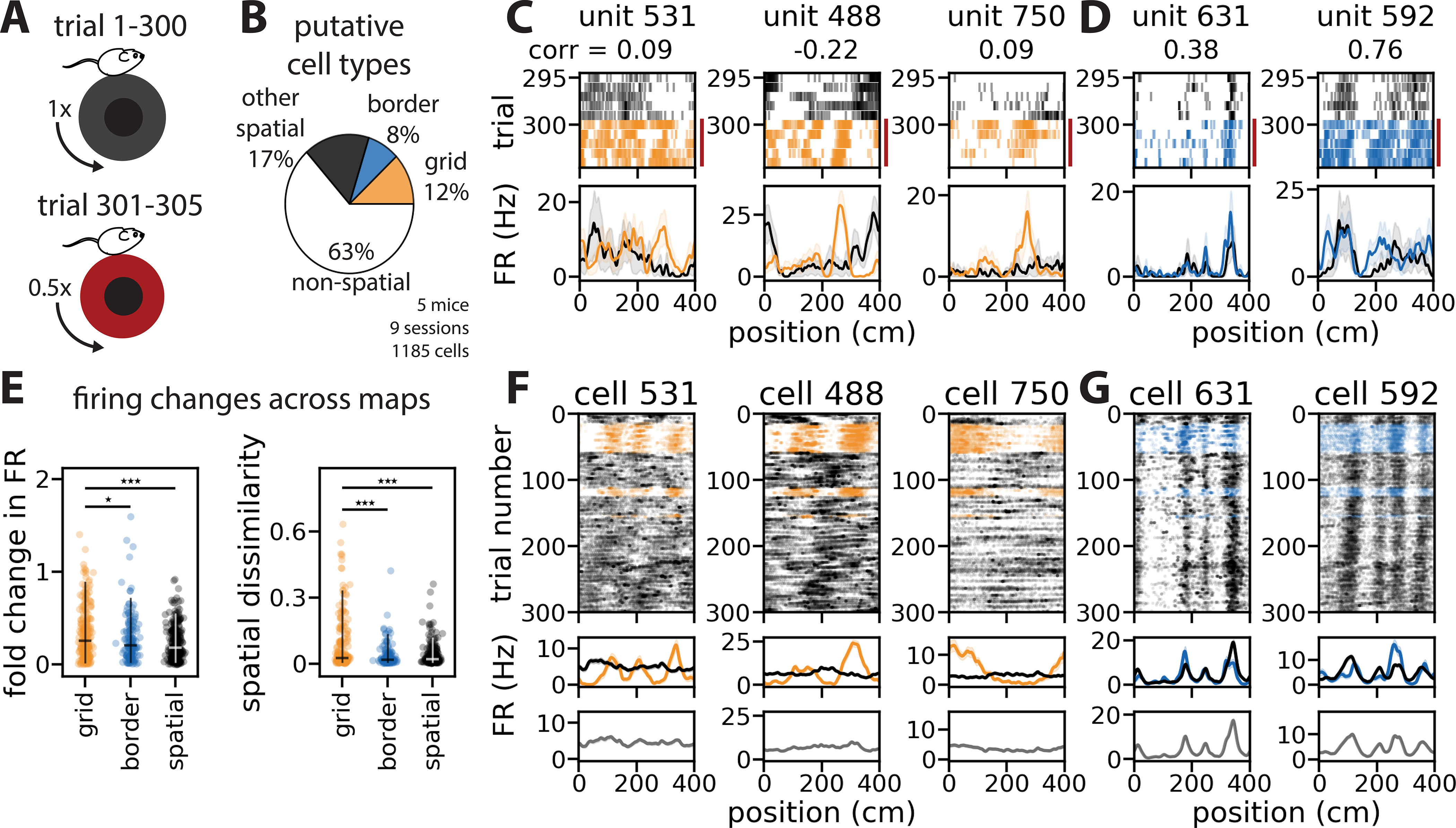
Figure 5: — (A) Schematized trial structure: 300 trials with a fixed relationship between visual and motor feedback (top, “normal trials”), 5 trials requiring the animal to run twice as far to travel the same visual distance (bottom, “gain change trials”). (B) Distribution of putative cell types (session mean ± SEM: grid cells, 18.26 ± 3.81%; border cells, 13.23 ± 2.07%; spatially stable cells, 24.57 ± 3.12%). (C) Rasters (top) and tuning curves (bottom) from example grid cells for adjacent normal (black) and gain change trials (red bar, colored spikes)(numbers indicate cell identity and correlation of tuning curves across gain change; solid line, average firing rate; shading, SEM). (D) Same as (C), but for example border cells. (E) Absolute fold change in firing rate (left)(median change, 95^th percentile: grid cells = 25.5%, 89.2%; border cells = 20.6%, 71.6%; other spatial cells = 18.5%, 55.5%; Kruskal-Wallis H-test, p = 4.6×10⁻⁴; Wilcoxon rank-sum test: border vs. grid cells, p = 0.045; other spatial vs. grid cells, p = 8.59×10⁻⁵; other spatial vs. border cells, p = 0.217) and cosine dissimilarity (right)(median, 95^th percentile: grid cells = 0.027, 0.334; border cells = 0.019, 0.137; spatial cells = 0.022, 0.119; Kruskal-Wallis H-test, p = 1.97×10⁻⁵; Wilcoxon rank-sum test: border vs. grid cells, p = 4.13×10⁻⁵; other spatial vs. grid cells, p = 1×10⁻⁴; other spatial vs. border cells, p = 0.227) across maps for all grid, border, and other spatial cell tuning curves (***, p < 0.001; *, p < 0.05). (F) Rasters (top) and tuning curves (middle) for example grid cells, colored by k-means cluster labels (color, map 1; black, map 2), versus averaged over the session (bottom)(solid line, trial-averaged firing rate; shading, SEM). (G) As in (F), but for example border cells. All example cells are from mouse 9b, session 1207_1 (n = 61 grid cells, 9 border cells, 165 total cells). (B, E) n = 224 grid cells, 152 border cells, 308 other spatial cells out of 1,1185 total excitatory cells from 9 cue rich sessions in 5 mice. Orange color denotes grid cells, blue denotes border cells throughout. (See also Figure S6.)

Positional information is conserved at a population level across distinct spatial maps

MEC neurons project to multiple brain areas involved in spatial information processing (Kerr et al., 2007). To consider how downstream brain areas might make use of positional information encoded in MEC in spite of network-level remapping, we investigated whether linear mechanisms can predict position from MEC neural activity by fitting circular-linear regression models (“decoders”) (Figure 6A–C; see Figure S5 for sessions with >2 maps)(STAR Methods). We found that performance was comparable between models trained and tested on trials from a single map, and models trained and tested on trials from both maps (p = 0.65)(Figure 6D). While remapping could disrupt the performance of a simple linear decoder if each neuron’s spatial tuning was sufficiently different across the maps, this finding may arise because only ~5% of cells showed large changes in spatial tuning across maps (Figure 4B). To simulate an alternative case where each neuron’s spatial tuning changed dramatically across maps, we produced a shuffled “synthetic map” for each of the two maps in which spatial coding was greatly altered (STAR Methods). Linear decoders trained jointly on data from each true map and its synthetic map performed substantially worse than decoders trained on data from the pair of true maps (p < 0.05)(Figure 6D).

Models also performed poorly when trained on data from one map and tested on data from the other map (p = 7.55×10⁻¹¹)(Figure 6E–F), though these decoders still largely outperformed a shuffle control (trained on one map, tested on a the shuffled other map; 3/56 model pairs were no better than shuffle, p ≥ 0.05)(Figure 6G; STAR Methods). Therefore the two maps are different—decoders specialized to a single map struggled to generalize to the other map (Figure 6E–G)—yet, given data from both maps, a single linear decoder performed as well as separate, specialized decoders (Figure 6D). Altogether, these results indicate that, in principle, downstream brain areas can exploit positional information encoded in MEC in the presence of remapping.

Neural activity transitions between geometrically aligned ring attractor manifolds

MEC representations of space thus can be both flexible (e.g. spontaneous remapping) and reliable (e.g. consistent decoding performance). To reconcile these two aspects of the circuit, we characterized the geometry of position coding in N-dimensional firing rate space (where N denotes the number of simultaneously recorded neurons). For the continuous 1D VR tracks used in this study, spatially driven network activity should follow a 1D ring manifold as the animal moves through space, reflecting the ring-shaped environment (Figure 7A). Attractor models of spatial navigation predict that circuit dynamics are locally stable around these ring manifolds, enabling persistent internal representations of position (Samsonovich and McNaughton, 1997). Each k-means cluster centroid provides an empirical estimate of this attractor manifold and, indeed, the low-dimensional linear embedding of each centroid had a qualitative ring structure (Figure 7B–C). Of note, we derived these ring-shaped manifolds from all co-recorded MEC neurons, making them distinct from the ring structures that arise in attractor models of co-modular grid cells (Burak and Fiete, 2009; Fuhs and Touretzky, 2006; Guanella et al., 2007; Spalla et al., 2019). Manifolds derived from cue poor environments were tightly wound around themselves, as quantified by an entanglement metric (Figure 7D; n = 10 manifolds from 5 cue poor sessions, 46 manifolds from 23 cue rich sessions)(see STAR Methods), indicating that there may be limited discriminability between the first and second halves of the track in this environment. These results suggest that the number of landmark cues alters the geometry of the spatial map without altering its topology as a 1D ring.

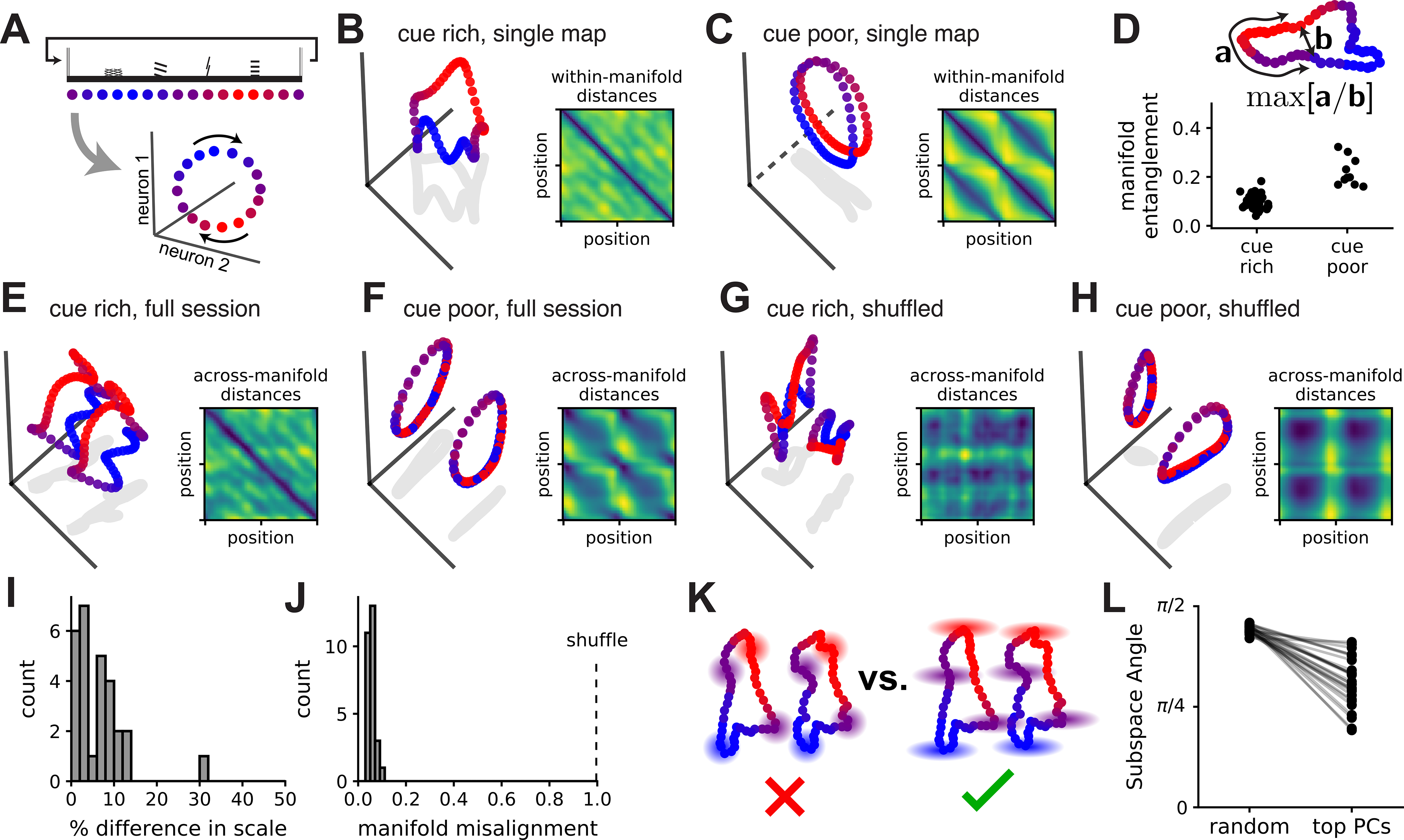
Figure 7: — (A) Schematic: the 1D environment (top) should produce a circular 1D trajectory (i.e., ring manifold) in neural activity space (bottom)(color scheme indicates position and is preserved throughout). (B) PCA projection of a single map (k-means centroid) from a cue rich session. (Inset) Pairwise distances in neural activity for all points (position bins) in the manifold (blue, minimum value; yellow, maximum). (C) As in (B), but for a cue poor session. The linear projection uses two principal components and a third orthogonal axis (dashed line) that maximally distinguishes between the first and second half of the track. (D)(Top) Schematic of the entanglement measure, which is the maximum ratio of distance along the manifold (“a”) to extrinsic distance (“b”)(STAR Methods). (Bottom) Manifold entanglement in cue rich and cue poor environments. (E) PCA projection of two manifolds from a 2-map cue rich session. (Inset) Across-manifold distances in neural firing rates for every pair of points (colors as in B, C insets). (F) As in (E), but for a cue poor session. (G, H) As in (E, F), respectively, but after randomly rotating each manifold. (I) Percent difference in manifold size for maps from the same session. (J) Normalized manifold misalignment scores (0, perfectly aligned; 1, shuffle). (K) Schematics: variability around the manifolds is oriented towards the other manifold (right), not isotropically distributed (left). (L) (Right) Angles between the remapping dimension and the top PC subspace for the model residuals (20% of total noise variance), (left) null distribution (random linear subspaces, n = 1,000 samples). All sessions displayed smaller angles than their shuffle control (Wilcoxon rank-sum test, p < 1×10⁻⁶). Example in (B, E, G) is session 1005_2 from mouse 6b (n = 149 cells) and in (C, F, H) is session 0502_1 from mouse 1c (n = 227 cells). (D, I, J, L) n = 46 manifolds from 23 cue rich sessions in 10 mice, 10 manifolds from 5 cue poor sessions in 3 mice.

We next used PCA to visualize the two manifolds of each 2-map session in the same low-dimensional space. In both cue rich and cue poor environments, the manifolds appeared geometrically aligned such that position coding was translated along a single dimension in neural activity space (Figure 7E–F), relative to a shuffle control (Figure 7G–H). Using Procrustes shape analysis (STAR Methods), we found that the two manifolds required only modest rescaling (23/28 sessions ≤ 10% difference in scale)(Figure 7I) and rotation (all were within 7% of the optimal rotation)(Figure 7J) to align with one another. This alignment could arise from preserved spatial tuning in some neurons and indicates that single neuron coding changes (Figure 4A–B) did not result in net firing rate differences across maps. Though tuning is correlated within grid cell modules (Hafting et al., 2005), manifold alignment was not dependent on putative grid cells (Figure S6). Thus, remapping largely corresponded to a translation in neural activity space between geometrically aligned ring manifolds.

As the k-means-identified ring manifolds show only the average neural activity within each map, we next asked how single-trial variability around these manifolds was structured. For each session, we applied PCA to the residuals of the k-means model and kept enough components to capture at least 20% of variance in these residuals. These dimensions contain the most “noise” or variability that isn’t captured by the k-means model. We then computed the angle between the PC subspace and the dimension separating the two manifolds (the “remapping dimension”); this was smaller than expected under a null distribution of random linear subspaces, indicating that unexplained neural variability was preferentially oriented in the remapping dimension (Figure 7K–L). The scale of this variability was limited so that the two manifolds were often well-separated (the maps can be considered two separate ring manifolds, rather than a single hollow cylinder). This result suggests that variability in network activity could predispose the network to remap (or jump from one ring manifold to the other), with attractor dynamics locally stabilizing the network activity within each map (Video S3).

A simple model explains the alignment of spatial attractor manifolds

Is the geometric alignment of spatial manifolds (Figure 7E–F) expected under existing theories of navigational circuit dynamics? To address this question, we constructed a bistable ring attractor model by linearly combining the weights of a winner-take-all network and a ring attractor network (Figure S7; STAR Methods). This approach is similar to previous models that have linearly combined decorrelated connectivity matrices to support multiple attractor structures (Romani and Tsodyks, 2010; Roudi and Treves, 2008; Samsonovich and McNaughton, 1997; Stringer et al., 2004). We could induce remapping in this model with perturbations that pushed the neural state into the other map’s basin of attraction (Monasson and Rosay, 2014, 2015). This model was sufficient to reproduce multiple ring manifolds, but it failed to recapitulate the experimentally observed geometrical manifold alignment (Figure S7). This finding demonstrates that geometrically aligned ring manifolds are not an obvious consequence of the attractor model framework.

A minor modification to this model—adding a sub-population of “shared neurons” whose spatial tuning was preserved across maps—was sufficient to produce a pair of bistable ring attractors that were highly aligned (Figure S7). This subpopulation is analogous to the experimentally observed neurons with preserved spatial tuning across maps (Figure 4A–B). The modified model had two additional noteworthy properties. First, perturbing the neural activity in the direction of the other map induced a remap but preserved the positional representation (Figure S7). Second, remapping was well-described by a translation along a single dimension; thus any spatial decoder that is insensitive to this dimension will be robust to remapping. For a linear decoder (as in Figure 6), this means the remapping dimension should lie in the null space of the decoder weights (Kaufman et al., 2014; Rule et al., 2020). Together, these results suggest that neurons with shared coding across maps may result in geometrically aligned ring manifolds, which in turn enables simple mechanisms for remapping and position decoding.

Remapping events and neural variability correlate with slower running speeds

As the task and environment in our experiments did not change within a given session, we next examined whether single-trial variability and network-wide remapping correlated with aspects of the animal’s behavior. We focused on running speed, as speed is known to modulate spatial representations in MEC (Bant et al., 2020; Hardcastle et al., 2017). We first asked whether the animal’s running speed was different on “remap trials” (the two trials book-ending each transition from one map to the other), compared to the intervening “stable blocks” (the block of trials at least two trials away from a remap event, which all reside in the same map). We restricted our analysis to 2-map sessions that contained at least three remap events and to stable blocks of at least five trials (n = 13 sessions in 7 mice; see Figure S5 for sessions with >2 maps)(STAR Methods). Across most of these sessions, the animal’s average running speed on remap trials was slower compared to its average running speed in the preceding stable block (difference in running speed: 9.8 ± 2.2%; p = 1.15×10⁻⁴)(Figure 8A, B). Running speed largely did not vary systematically across the two maps (Figure S8)(STAR Methods).

Figure 8: — (A) Average running speed in remap trials versus stable blocks for an example session (points, pairs of remap trials/stable blocks; dashed line, unity; n = 13 pairs) (B) As in (A), but for all 2-map sessions (remap trial speeds were slower in 9 sessions, equal in 2 sessions, faster in 2 sessions; Wilcoxon signed-rank test, p = 1.15×10⁻⁴)(points, session average; green, cue poor; pink, cue rich; grey error bars, SEM; dashed line, unity; n = 127 pairs from 13 sessions, 7 mice). (C) (Top and bottom panels) Running speed and distance to the midpoint between k-means clusters for trials from two example stable blocks (black trace, running speed; black shading, map 1; white, map 2; gray, between maps). (Middle panels) Zoom in on the first (left) and last (right) example trials, showing neural activity approaching the midpoint (arrowheads)(across sessions, stable bin distance interquartile range: 0.763 to 1.338). (D) Average distance to the midpoint versus binned running speed for an example session (distance score = 1, activity is in a cluster centroid; 0, equidistant from each map)(black line, average; gray shading, SEM; distance to midpoint is z-scored). (E) as in (D), but for all 2-map sessions; speed is normalized within each session (ordinary least squares regression, R² = 0.778, p < 1×10⁻⁶; n = 10 speed bins per session, 28 sessions, 13 mice, 4,984 cells). (F) Schematic model showing how running speed might encourage neural activity (ball, activity; arrow, trajectory in state space) to transition between manifolds (top) by shaping the energy landscape (black line)(middle, slow speeds; bottom, fast; dashed line, midpoint between clusters). Example session in (A, C, D) is from mouse 1c, session 0430_1 (n = 227 cells). (See also Figure S5, S8.)

We next investigated the moment-by-moment correlation between neural variability and running speed by binning neural activity and speed into 5 cm position bins within each trial. Given the random reward structure, the running speed distribution for each track position was comparable (Figure S8). For each position bin, we calculated how close the neural activity was to the midpoint between manifolds, where activity is most likely to switch between maps (STAR Methods). As expected, neural activity was closer to the midpoint in remap trials compared to stable blocks (p < 1×10⁻⁶)(Figure S8). However, we also observed instances where the neural activity approached the midpoint within stable periods, indicating that neural variability does not always provoke a remap event (Figure 8C, arrowheads). Across all position bins, slower running speeds were correlated with a reduced neural distance to the midpoint (p < 1×10⁻⁶)(Figure 8D, E). Altogether, these results suggest that neural variability increases in the direction of the other map at slow running speeds, likely increasing the probability of a remap event. If we model the two spatial maps as bistable ring attractors (as discussed in the previous section), then a decrease in running speed could correspond to a reduction in the energetic barrier that separates the two basins of attraction (Figure 8F) or to another change that encourages neural activity to flip to the other attractor. Although the neural distance to the midpoint between clusters was variable across different track positions and appeared to dip slightly in the reward zone, this variability was no greater than expected by chance (p > 0.05)(Figure S8).

Discussion

Here, we report that MEC representations are capable of remapping in VR environments without any changes to sensory cues (Diehl et al., 2017; Fyhn et al., 2007; Marozzi et al., 2015; Solstad et al., 2008) or task demands (Boccara et al., 2019; Butler et al., 2019; Keene et al., 2016). Remapping events were coordinated across the MEC population, recruited many different cell types, and often comprised discrete and reversible switches between spatial maps that persisted over long (roughly 1–30 min) timescales. Remapping comprised diverse coding changes across neurons—including up to three-fold variation in peak firing rate and 50% reconfiguration of spatial coding—and appeared to differentially impact different functional cell types. While previous reports have found that faster running speed is associated with sharpened spatial tuning in single neurons (Bant et al., 2020; Hardcastle et al., 2017), we found that changes in running speed can also correspond to remapping events that produce large and persistent shifts in MEC coding. Finally, neural activity remapped by transitioning between geometrically aligned manifolds, enabling simple, linear decoding strategies. Together, our results suggest that a single population of MEC neurons can rapidly switch between multiple stable representations of a single environment.

While neural activity often alternated between two stable spatial maps, we also observed sessions with more than two stable maps and sessions where activity remapped between spatially stable and unstable coding regimes. We largely focused on single-track sessions with two maps (“2-map sessions”), which allowed us to thoroughly characterize this common form of remapping and provided insight into how neural circuits might store and interpret multiple neural representations more generally. We found that a single decoder could accurately infer position across remapping events, indicating that MEC spatial representations contain both changing contextual information and stable positional information that is segregated into orthogonal linear subspaces (Kaufman et al., 2014; Rule et al., 2020). Our finding that remapping comprised a translation in neural activity space provides a geometric interpretation for this possibility. This geometric arrangement could allow downstream neurons that are insensitive to the remapping dimension to extract consistent positional information regardless of the map, while neurons sensitive to this dimension could extract contextual information.

We further showed that a bistable ring attractor model network (Battaglia and Treves, 1998; Romani and Tsodyks, 2010; Samsonovich and McNaughton, 1997) does not produce aligned rings, but that adding a sub-population of “shared neurons” was sufficient to recapitulate the experimentally observed alignment. Previous work has studied transitions between continuous attractors in the context of hippocampal and co-modular grid cell attractor networks (Monasson and Rosay, 2014, 2015; Spalla et al., 2019). Our modeling results differ by (1) considering the full MEC circuit (not only grid cells) and (2) interpreting each continuous attractor as representing the same external environment (not different environments). Overall, these results illustrate how our experimental findings might be interpreted and integrated into ongoing theoretical research on MEC and hippocampal circuits.

One feature of remapping between aligned manifolds is that it allows the network to preserve unchanging information while rapidly and synchronously updating changing contextual information. Our findings complement previous studies in the hippocampus (Rubin et al., 2015; Taxidis et al., 2020; Ziv et al., 2013) and MEC (Diehl et al., 2019), which found context delineation in a single environment over longer timescales (hours to days) via representational drift that is asynchronous across neurons. This type of remapping over longer timescales may relate to learning dynamics (Taxidis et al., 2020), grouping of temporally adjacent memories (Rubin et al., 2015), and building an episodic timeline for repeated interactions with a single environment (Diehl et al., 2019; Sheintuch et al., 2020; Ziv et al., 2013). The rapid remapping (under 1 min) that we observed across MEC may interact with these slower processes of representational drift to form a rich internal map of temporal and contextual episodes.

Of note, it is possible that the impoverished sensory experience of our virtual environment promoted remapping, perhaps leading the animal to infer multiple different contexts in the same VR track (Ravassard et al., 2013; Sanders et al., 2020). However, complete remapping of hippocampal spatial representations of a single environment was recently observed in freely behaving animals, suggesting that similar remapping can occur under more naturalistic settings (Sheintuch et al., 2020). It is also well-established that MEC neurons can remap in freely behaving animals in response to changing sensory features (Diehl et al., 2017; Fyhn et al., 2007; Marozzi et al., 2015; Solstad et al., 2008) or task demands (Boccara et al., 2019; Butler et al., 2019; Keene et al., 2016). Our findings may represent a related form of MEC remapping that is driven by internal, rather than external factors, which likely interacts with previously established forms of remapping.

Finally, our finding that remapping events correlated with slower running speeds raises specific hypotheses for how behavioral state may drive widespread changes in MEC coding. Running speed can indicate task engagement—e.g., in our task faster speeds lead the animal to “find rewards” more quickly—or of arousal more broadly (Bennett et al., 2013; Niell and Stryker, 2010)(but see Vinck et al., 2015). Behavioral state changes related to running speed and arousal can alter neural processing in complex ways; for example targeted neuromodulation of GABAergic interneurons modulates sensory neuron responses (Ferguson and Cardin, 2020). It is possible that similar or analogous biophysical mechanisms act on MEC neurons and it will be of particular interest for future studies to dissect the mechanisms by which MEC neurons are commonly and differentially impacted by running speed. Moreover, detailed consideration and tracking of multiple behavioral state variables (e.g. pupil dilation and whisking) will be needed to identify which specific variables control remapping in the navigation circuitry.

Altogether, we find that MEC has the capacity to remap in a rapid and reversible fashion, which could support a role for this circuit in dividing the unbroken stream of sensory features encountered during navigation into discrete contextual episodes. Further, our findings align with a larger body of emerging studies demonstrating that cortical activity is highly responsive to behavioral state changes (Jennings et al., 2019; Salay et al., 2018; Stringer et al., 2019). Our results suggest that these behavioral state changes may drive rapid, large-scale reconfigurations of internal representations of the external world in higher-order cortex.

STAR Methods

Resource Availability

Lead Contact:

Further information and requests for resources and reagents should be directed to and will be fulfilled by the Lead Contact, Lisa M. Giocomo (giocomo@stanford.edu).

Materials Availability:

This study did not generate new unique reagents.

Data and Code Availability

All data required to reproduce the paper figures have been deposited at Mendeley and are publicly available as of the date of publication. DOIs are listed in the key resources table.
All original code has been deposited at Zenodo and is publicly available as of the date of publication. DOIs are listed in the key resources table.
Any additional information required to reanalyze the data reported in this paper is available from the lead contact upon request.

KEY RESOURCES TABLE.

REAGENT or RESOURCE	SOURCE	IDENTIFIER
Deposited data
Raw and analyzed data	This paper	https://data.mendeley.com/10.17632/hntn6m2pgk.1
Experimental models: Organisms/strains
Mouse: C57BL/6	The Jackson Laboratories	000664
Software and algorithms
SciPy ecosystem of open-source Python libraries (numpy, matplotlib, scipy, etc.)	Jones et al., 2001; Hunter, 2007; Harris et al., 2020	https://www.scipy.org/
scikit-learn	Pedregosa et al., 2011	https://www.scikit-learn.org/
MATLAB	MathWorks	https://www.mathworks.com/products/matlab.html
Kilosort2		https://github.com/MouseLand/Kilosort2
Other
Phase 3B Neuropixels 1.0 silicon probes	Jun et al., 2017	https://www.neuropixels.org/probe
Original code	This paper	https://doi.org/10.5281/zenodo.5062491

Open in a new tab

Experimental Model and Subject Details

Mice

All techniques were approved by the Institutional Animal Care and Use Committee at Stanford University School of Medicine. Recordings were made from 17 C57BL/6 mice aged 4 weeks to 3.5 months at the time of first surgery (15.7–35 g). All mice were female except litters 5 and 9 (6 mice), which were male. Mice were group housed with same-sex littermates, and in one case with the dam (2a, b, c with 3a), unless separation was required due to water restriction, aggression, or disturbance of prep site. Mice were housed in transparent cages on a 12-h light-dark cycle and experiments were performed during the light phase.

Method Details

Training and handling

Mice were handled at least every 2 days following headbar implantation and given an in-cage running wheel. Starting 1 day after headbar implantation, same-sex mice were placed daily in a large (100×100cm), communal environment with enrichment objects including a running wheel, Lego tower, textured floor tape, and crushed chocolate cheerios for between 15 mins and 2 hours. Mice were monitored for aggression and separated as needed. Mice were given free access to water until 3 days after headbar implantation, after which they were water restricted to 1mL of water per day and weighed daily to ensure a body weight of >80% of their starting weight.

After >1 day of water restriction, mice were acclimated to head fixation and trained to drink water from a custom lickport for 10–20 mins over 2 days. Mice were then trained to run on the virtual random forage task (described below) starting with a reward probability of 0.1/cm (essentially one reward per 50 cm), for gradually decreasing reward probability and gradually increasing session length as behavior improved. Mice were trained on the exact track(s) that they were recorded in, either cue poor (litters 1, 2, and 3), cue rich (litters 6, 7, 9 and 10), or both (litters 4 and 5). Mice trained on both tracks were exposed to each track in a counterbalanced fashion, initially alternating tracks over days and ultimately alternating the order of presentation as mice improved sufficiently to run 2 or more sessions per training day. Training continued at least until mice ran >300 trials in 2 hours and demonstrated proficient licking from the lickport in the reward zone; training was sometimes extended in order to stagger recording periods (7 days to 7 weeks; mean ± SEM: 23 ± 3 days; 7 mice never learned the task).

In vivo survival surgeries

For all surgeries, anesthesia was induced with isoflurane (4%; maintained at 0.5–1.5%) followed by injection of buprenorphrine (0.05–0.1 mg/kg). Animals were injected with baytril (10 mg/kg) and rimadyl (5 mg/kg) immediately following each surgery and for 3 days afterwards. In the first surgery, animals were implanted with a custom-built metal headbar containing two holes for head fixation, as well as with a jewelers’ screw with an attached gold pin, to be used as a ground. The craniotomy sites were exposed and marked during headbar implantation and the surface of the skull was coated in metabond. After completion of training, a second surgery was performed to make bilateral craniotomies (~200μm diameter) at 3.7–3.95mm posterior and 3.3–3.4mm lateral to bregma. A small plastic well was implanted around each craniotomy and affixed with metabond. Craniotomy sites were covered with a drop of sterile saline and with silicone elastomer (Kwik-sil, WPI) in between surgery and recordings.

In vivo electrophysiological data collection

All recordings were performed at least 16-h after craniotomy surgery. Mice were head-fixed on the VR recording rig. Craniotomy site was exposed and rinsed with saline—occasionally dura was re-nicked or debris removed using a syringe tip. Recordings were performed using Phase 3B Neuropixels 1.0 silicon probes (Jun et al., 2017) with 384 active recording sites (out of 960 total) along the bottom ~4 mm of a ~10 mm shank (70 μm wide shank diameter, 24 μm thick, 25 μm electrode spacing), and reference and ground shorted together. The probe was positioned over the craniotomy site at 8–14° from vertical and targeted to ~50–300 μm anterior of the transverse sinus using a micromanipulator. On consecutive recording days, probes were targeted medial or lateral of previous recording sites as permitted by the craniotomy and/or probe angle was varied to ensure that we were recording from a new population of cells each day (Figure S1). The reference electrode was then connected to a gold ground pin implanted in the skull. The probe was advanced slowly (~4–10 μm/s) into the brain until it encountered resistance or until activity quieted on channels near the probe tip, then retracted 100–500μm and allowed to sit for at least 30 mins prior to recording. While the probe was implanted, the craniotomy site was covered with sterile saline and silicon oil. Signals were sampled at 30 kHz with gain = 200 (7.63 μV/bit at 10 bit resolution) in the action potential band, digitized with a CMOS amplifier and multiplexer built into the electrode array, then written to disk using SpikeGLX software.

Virtual reality (VR) environment

The VR recording set-up was nearly identical to the set-up in Campbell et al. (Campbell et al., 2018). Head-fixed mice ran on a 15.2-cm-diameter foam roller (ethylene vinyl acetate) constrained to rotate about one axis. The cylinder’s rotation was measured by a high-resolution quadrature encoder (Yumo, 1024 P/R) and processed by a microcontroller (Arduino UNO). The virtual environment was generated using commercial software (Unity 3D) and updated according to the motion signal. VR position traces were synchronized to recording traces on each frame of the virtual scene. The virtual scene was displayed on three 24-inch monitors surrounding the mouse. The gain of the linear transformation from ball rotation to translation along the virtual track was calibrated so that the virtual track was 4 m long. At the end of the track, the mouse was teleported seamlessly back to the start to begin the next trial, such that the track was seemingly infinite (all visual cues were repeated and visible into the distance as the mouse approached the track end).

Cue rich tracks consisted of 5 towers of different heights, widths, and patterns (black and white, neutral luminance), placed at 80 cm intervals starting at 0 cm and a black and white checkerboard on the floor for optic flow (see schematic, Figure 1B, top, and screenshot, Figure S1A). Cue poor tracks contained 2 towers of different patterns placed at 0 and 200 cm and a white to black horizontal sinusoidal pattern on the floor (see schematic, Figure 1B, bottom, and screenshot, Figure S1B). Both tracks had uniform gray walls and sky beyond the towers. For mice that experienced a single track, recording sessions consisted of 57–450 trials (mean ± SEM: 328 ± 14 trials). For mice that experienced both tracks, each track was presented in a block of 75–100 trials with ~1 min of darkness in between tracks (Figure S8). Blocks alternated between cue rich and poor—each track was presented twice (barring rare cases when the mouse failed to complete the session) and which track was presented first was alternated on each day.

In a subset of cue rich, single-track sessions (N = 21 sessions in 5 mice) we appended 5 gain manipulation trials to the end of each session in which the mouse had to run twice as far to traverse the same distance along the virtual track, as in Campbell et al. (Campbell et al., 2018).

Random foraging task

In both cue rich and cue poor tracks, visually marked reward zones appeared at a probability of 0.01–0.001 per cm, titrated to mouse performance, within the middle 300 cm of the track and at least 50 cm apart. Reward zones were 50 cm long and track-width, were patterned with a black and white diamond checkerboard, and hovered slightly above the floor (Figure S1). Upon entering the reward zone, animals could request water by licking and breaking an infrared beam at the mouth of the lickport; if not requested, water was dispensed automatically at the center of the zone. For mice 1c, 4a, and 4b for some recording sessions there were between 1–5 probe trials every 10 trials in which water was only dispensed if requested in the reward zone (no automatic dispensation). Upon water dispensation (or next trial start for missed probe trials), the current reward zone disappeared and the next zone became visible. Water rewards (~1.5 μL) were delivered using a solenoid (Cole-Parmer) triggered from the virtual environment software, generating an audible click with water delivery. Licks were recorded as new breaks in the lickport infrared beam and were processed by a microcontroller (Arduino UNO).

Histology and probe localization

Before each implantation, probes were dipped in fixable lipophilic dye (1mM DiI, DiO, DiD, Thermo Fisher) 10 times at 10 second intervals. Within 7 days of the first probe insertion, mice were killed with an overdose of pentobarbital and transcardially perfused with phosphate-buffered saline (PBS) followed by 4% paraformaldehyde. Brains were extracted and stored in 4% paraformaldehyde for at least 24 h before transfer to 30% sucrose in PBS. Brains were then rapidly frozen, cut into 30-μm sagittal sections with a cryostat, mounted and stained with DAPI. Histological sections were examined and the location of the probe tip and entry into the dorsal MEC for each recording were determined based on the reference Allen Brain Atlas (Allen Institute for Brain Science, 2004)(Figure S1). The location of each recording site along the line delineated by the probe tip and entry point was then determined based on each site’s distance from the probe tip. Only cells within MEC, again based on the reference Allen Brain Atlas (Allen Institute for Brain Science, 2004), were included for analysis (Figure S1). In all cases, “depth” reported is the ventral distance from the dorsal boundary of MEC in the medial section where the probe entered MEC.

Offline spike sorting

Electrophysiological recordings were common-average referenced to the median across channels and high-pass filtered above 150 Hz. Automatic spike sorting was then performed using Kilosort2, a high-throughput spike sorting algorithm that identifies clusters in neural data and is designed to track small amounts of neural drift over time (open source software by Marius Pachitariu, Nick Steinmetz, and Jennifer Colonell, https://github.com/MouseLand/Kilosort2)(see also Kilosort1 (Pachitariu et al., 2016)). After automatic spike-sorting, all clusters with peak-to-peak amplitude over noise ratio < 3 (with noise defined as the standard deviation of voltage traces in a 10ms window preceding detected spike times), total number of spikes < 100, and repeated refractory period violations (0–1 ms autocorrelegram bin > 20% of maximum autocorrelation) were excluded. All remaining clusters were manually examined and labeled as “good” (i.e., stable and likely belonging to a single, well-isolated neural unit), “MUA” (i.e., likely to represent multi-unit activity), or “noise.” Only well-isolated “good” units from within MEC (barring Figure S1I–J, which were non-MEC units) with greater than 400 spikes were included for analysis in this paper (Figure 1G). Sessions with fewer than 10 cells meeting these criteria were excluded.

Behavioral data preprocessing

On each frame of the virtual reality scene, the virtual position and time stamps were recorded and a synchronizing TTL pulse was sent from an Arduino UNO to the electrophysiological recording equipment. These pulses were recorded in SpikeGLX using an auxiliary National Instruments data acquisition card (NI PXIe-6341 with NI BNC-2110). The location of each reward zone, time of each lick, and time of each reward dispensation were also recorded. Thus all time stamps and behavioral factors were synchronized to the neurophysiological data. Time stamps were adjusted to start at 0 and all behavioral data was interpolated to convert the variable VR frame rate to a constant frame rate of 50Hz. As the track was effectively circular and 400 cm long, recorded positions less than 0 or greater than 400 cm were converted to the appropriate position on the circular track (eg. a recorded position of 404 cm would be converted to 4 cm and a recorded position of −4 cm would be converted to 396 cm). Trial transitions were identified as timepoints where the difference in position across time bins was less than −100 cm (i.e., a transition from ~400 cm to ~0 cm) and a trial number was accordingly assigned to each timepoint.

Running speed for each timepoint was computed by calculating the difference in position between that timepoint and the previous, divided by the framerate (speed at the first timepoint was assigned to be equal to that at the second timepoint). Speeds greater than 150 cm/s or less than −5 cm/s were removed. Speed was then interpolated to fill removed timepoints and smoothed with a gaussian filter (standard deviation 0.2 time bins). For all analyses except lick and reward zone analyses (Figure 1C–F), stationary time bins (speed < 2 cm/s) were excluded.

Running speed across maps

Because the k-means cluster labels are arbitrarily assigned, we designated the map with the slower overall average running speed as map 1 for consistency across analyses. To assess possible differences in running speed across maps, we computed the fractional difference in running speed across the k-means identified maps in all 2-map sessions. To control for any systematic changes in running speed over time in the session, we calculated the average running speed for each block of adjacent trials from the same map and compared it to the average running speed of the subsequent block of trials from the other map. We compared the resulting distribution of fractional difference in running speed to a shuffle control in which running speed was randomly shuffled across time bins (re-designating map 1 according to whichever shuffled map had a slower overall average running speed; 1000 shuffles per session)(Figure S8J).

Population analysis and clustering model

The 1D track was divided into 5 cm position bins (total of 80 bins). On each traversal of the track, the empirical firing rate of each neuron—i.e., number of spikes divided by time elapsed—was computed for every position bin. We then smoothed the firing rate traces with a Gaussian filter (standard deviation 5 cm). For each session this resulted in a 3-dimensional array of raw firing rates, with dimensions corresponding to trials, positions, and neurons.

Because these raw firing rates varied widely across neurons, we rescaled them so that the peak firing rate was commensurate across cells. Similar normalization steps or variance-stabilizing transformations have been used in previous population analyses of neural data (Churchland et al., 2012; Williams et al., 2018; Yu et al., 2009), to prevent neurons with high firing rates from washing out low firing rate neurons. Here, we normalized firing rates by first clipping the maximum firing rate of each neuron at its 90th percentile (to exclude large outliers), and then re-scaling each neuron’s firing rate to range between zero and one. That is, if ${\tilde{X}}_{i j k}$ denotes the clipped firing rate on trial i, position bin j, and neuron k, then the normalized firing rate was computed as:

X_{i j k} = \frac{{\tilde{X}}_{i j k} - \min ({\tilde{X}}_{: : k})}{\max ({\tilde{X}}_{: : k}) - \min ({\tilde{X}}_{: : k})}

(1)

The max(·) and min(·) operations (as well as the 90th percentile clipping operation) are applied on a neuron-by-neuron basis, pooling observations across all trials and timebins. For double-track sessions (which contained 2 blocks of cue rich trials and 2 blocks of cue poor trials, in alternating order) we added an additional per-neuron correction factor to account for drift in firing rates: the mean normalized firing rate for each neuron (across all trials and position bins) was subtracted within each block of trials, and the result was renormalized to values between zero and one, as above.

On each trial, MEC’s representation of position is summarized by a matrix, denoted X_i∷ for trial i, with rows and columns respectively corresponding to position bins and neurons. A simple measure of similarity between two trials, indexed by i and i′, is given by the Pearson correlation between the vectors vec(X_i∷) and $v e c (X_{i^{'} : :})$ . Network-wide trial-by-trial similarity matrices (as in Figure 2, 3, S1, S2, S4, and S5) were found by computing this correlation across all pairs of trials.

Let X_ijk denote the I × J × K array, or tensor, of normalized firing rates defined in equation (1). As before the index variables i, j, and k, respectively represent trials, position bins, and neurons. Now consider the following low-rank matrix factorization model (Singh and Gordon, 2008; Udell et al., 2016) of these data:

{\hat{X}}_{i j k} = \sum_{r = 1}^{R} U_{i}^{(r)} V_{j k}^{(r)}

(2)

Where R < min(I, J, K) denotes the number of model components, or the model rank. Equation (2) represents an approximate factorization of the I × JK matricization or tensor unfolding of the data array (Kolda and Bader, 2009; Seely et al., 2016). We will see that k-means clustering arises as a special case of this model, and in this special case R represents the number of clusters (i.e., the number of spatial maps).

The parameters $U_{i}^{(r)}$ and $V_{j k}^{(r)}$ are optimized according to a least squares criterion:

minimize \sum_{ijk} {(\sum_{r = 1}^{R} U_{i}^{(r)} V_{j k}^{(r)} - X_{i j k})}^{2}

(3)

It is well-known that a rank-R truncated singular value decomposition (SVD) provides a solution to this optimization problem (Eckart and Young, 1936). Further, the solution provided by truncated SVD is closely related to Principal Components Analysis (PCA)—indeed, these two methods are identical for the case of mean-centered data (see, e.g., (Shlens, 2005)). Since the normalized firing rate array X_ijk in equation (3) is not mean-centered, we refer to this initial model as “uncentered PCA.” We use the uncentered coefficient-of-determination (uncentered R²) as a normalized measure of model performance associated with equation (3).

The k-means clustering model incorporates an additional constraint into the uncentered PCA model. Specifically, k-means seeks to minimize equation (3),

subject to \sum_{r} U_{i}^{(r)} = 1 for all i \in {1, \dots, I}, and U_{i}^{(r)} \in {0, 1} for all i, r \in {1, \dots, I} \times {1, \dots, R}

(4)

Thus, if we view $U_{i}^{(r)}$ as the elements of an R × I matrix, the rows of this matrix are constrained to be standard Cartesian basis vectors of R-dimensional space (“one-hot vectors”). Each of these vectors specifies the cluster assignment label for every trial (see Figure 3A for a schematic illustration for the R = 2 case). Further, we can interpret $V_{j k}^{(r)}$ as elements of an R × J × K array. For a fixed cluster index r, the remaining elements form a J × K matrix, called a “slice” of the original array (Kolda and Bader, 2009). Each slice corresponds to a cluster centroid, which we may interpret as a spatial map—the columns are J-dimensional vectors holding the spatial tuning curves for every neuron, so different slices correspond to different sets of spatial tuning curves (i.e., different spatial maps).

This connection between k-means clustering and other matrix factorization models is well-known and expanded upon in detail by (Singh and Gordon, 2008; Udell et al., 2016). We exploit this connection to assess the k-means model, which is more constrained than uncentered PCA (i.e., truncated SVD) in that each row of $U_{i}^{(r)}$ is constrained to be a one-hot vector as opposed to an arbitrary vector. Intuitively, this allows us to interpret each trial as belonging to one of R types, as opposed to a linear combination of them. The fact that the more restrictive k-means model performs nearly as well as uncentered PCA gives credence to the multiple-map interpretation. To compare these two models we used a randomized cross-validation procedure in which 10% of the data, representing the validation set, were censored in a speckled holdout pattern (Williams et al., 2018; Wold, 1978). Ten randomized replicates were performed for all models. For the case of R = 2 components, we often observed similar performance (measured by the uncentered R² averaged over validation sets) between uncentered PCA and k-means for all sessions (Figure 3C). Further, we compared the test performance of k-means on “shuffled” datasets (Figure 3C right, Figure 3D). Firing rates from a behavioral session were shuffled by applying a random rotation (i.e., an orthogonal linear transformation) to X_ijk across trials. That is, we sample a random rotation matrix $Q_{i i^{'}}$ and define

X_{i j k}^{*} = \sum_{i^{'} = 1}^{I} Q_{i i^{'}} X_{i^{'} j k}

as the new shuffled dataset, which is substituted into the objective function defined in equation (3). This form of shuffling preserves many features of the data, including the overall norm of the data and correlations between neurons and position bins. However, it destroys the sparsity pattern on $U_{i}^{(r)}$ which is imposed by the k-means model. This procedure is similar in spirit to methods proposed by Elsayed & Cunningham (2017).

Sessions that were well-approximated by the k-means model with R = 2 clusters were classified as “two-map” sessions (Figure 3D). We required that the performance gap (measured by the uncentered R² averaged over validation sets) between k-means and uncentered PCA and be less than 70% relative to the shuffle control. Further, we required an uncentered R² of at least 0.63 for the k-means model with R = 2 maps. Sessions not meeting these criteria sometimes displayed more than two maps (see Figure S5), long periods of unstable coding (see Figures S1 and S2), or little to no remapping at all (Figure S2). For all k-means analyses, we ran the clustering model at least 100 times on all neural data from each session to account for model variability, keeping the model with the best fit to the data.

Manifold alignment analysis

We used standard Procrustes analysis methods (Gower and Dijksterhuis, 2004) to assess the degree to which the two ring manifolds, representing spatial maps, were aligned in neural firing rate space. Recall that the k-means centroids provide an estimate of each spatial map—in this case, we restrict our focus to R = 2 maps, so the two maps are given by $V_{j k}^{(1)}$ and $V_{j k}^{(2)}$ . Geometrically, these maps are represented as J points embedded in a K-dimensional space (recall that J denotes the number of position bins and K is the number of simultaneously recorded neurons). Procrustes Analysis begins by centering each of these manifolds at the origin and rescaling them to have unit norm. Let ${\bar{V}}_{j k}^{(1)}$ and ${\bar{V}}_{j k}^{(2)}$ denote the maps after these preprocessing steps have been applied, i.e.,

{\bar{V}}_{j k}^{(1)} = \frac{V_{j k}^{(1)} - \frac{1}{J} \sum_{j} V_{j k}^{(1)}}{{(\sum_{j k} {(V_{j k}^{(1)} - \frac{1}{J} \sum_{j} V_{j k}^{(1)})}^{2})}^{1 / 2}}

{\bar{V}}_{j k}^{(2)} = \frac{V_{j k}^{(2)} - \frac{1}{J} \sum_{j} V_{j k}^{(2)}}{{(\sum_{j k} {(V_{j k}^{(2)} - \frac{1}{J} \sum_{j} V_{j k}^{(2)})}^{2})}^{1 / 2}}

Since position bin j in map 1 and position bin j in map 2 correspond to the same location on the track, we consider the root-mean-squared-error (RMSE) between these centered and rescaled maps as the empirically “observed” alignment score (reported in Figure 5J):

{(\frac{1}{J K} \sum_{j k} {({\bar{V}}_{j k}^{(1)} - {\bar{V}}_{j k}^{(2)})}^{2})}^{1 / 2}

The central step of Procrustes analysis is to find the optimal rotation matrix that aligns these two point clouds. That is, we wish to find the matrix $Q_{k k^{'}}^{*}$ that solves the following optimization problem:

\begin{array}{l} minimize \sum_{j k} {({\bar{V}}_{j k}^{(1)} - \sum_{k^{'}} Q_{k k^{'}} {\bar{V}}_{j k^{'}}^{(2)})}^{2} \\ subject to \sum_{k} Q_{ℓ k} Q_{k p} = δ_{ℓ p} for all ℓ, p \in {1, \dots, K} \times {1, \dots, K} \end{array}

This optimization problem admits a closed form solution that is expressed in terms of the singular value decomposition of the K × K matrix $\sum_{j} {\bar{V}}_{j k}^{(1)} {\bar{V}}_{j k^{'}}^{(2)}$ (Schönemann, 1966). See Gower & Dijksterhuis (Gower and Dijksterhuis, 2004) for further background material. In Figure 7J, we report the RMSE compared to the optimal rotation (misalignment score = 0) and a random rotation matrix (“shuffle”).

Manifold entanglement calculation

We quantified the entanglement of a manifold as the maximum ratio of intrinsic distance (i.e., distance along the manifold) to extrinsic distance (i.e., Euclidean distance in K-dimensional space) between any two points on the manifold. Concretely, the extrinsic distance between two points corresponding to position bins j and j′ was computed as:

d_{j j^{'}} = {(\sum_{k} {(V_{j k} - V_{j^{'} k})}^{2})}^{1 / 2}

The intrinsic distance, $D_{j j^{'}}$ , was the sum of extrinsic distances along the shortest path from j to j′ (see diagram in Figure 7D). Depending on whether one travels clockwise or counterclockwise along the ring, there are two paths connecting any pair of points—the intrinsic distance is given by whichever path is shorter. The triangle inequality implies that $D_{j j^{'}} \geq d_{j j^{'}}$ for every pair of points along the manifold. When the ratio $D_{j j^{'}} / d_{j j^{'}}$ is large, this implies that the pair of points (j, j′) on the manifold are close together in neural firing rate space despite encoding very different positions on the VR track—speaking loosely, we say these points are “entangled.” Conversely, when $D_{j j^{'}} / d_{j j^{'}}$ is small, the two points are far apart in firing rate space in proportion to their encoded positions on the VR track. Thus, a measure of manifold entanglement is given by $\max [D_{j j^{'}} / d_{j j^{'}}]$ , which measures the worst-case entanglement over the full manifold (the max[·] operator is understood to be taken over all pairs of position bins, j and j′). Noting that this raw entanglement score is upper bounded by $B = \max [D_{j j^{'}}] / \min [d_{j j^{'}}]$ and lower bounded by one, we can normalize the tangling metric to range between zero (no entanglement) and one (high entanglement) as follows:

\frac{\max [D_{j j^{'}} / d_{j j^{'}}] - 1}{B - 1}

We report this normalized entanglement metric in our results.

Distance to cluster calculations

After fitting the k-means model and obtaining two centroids, $V_{j k}^{(1)}$ and $V_{j k}^{(2)}$ , we can quantify how close network activity is to each centroid on a trial-by-trial or neuron-by-neuron basis. In each case we project the activity onto a one-dimensional space where −1 corresponds to one centroid and +1 corresponds to the other centroid. That is, for each trial i, we compute

P_{i} = \frac{\sum_{j k} (2 X_{i j k} - (V_{j k}^{(1)} + V_{j k}^{(2)})) (V_{j k}^{(1)} - V_{j k}^{(2)})}{\sum_{j k} {(V_{j k}^{(1)} - V_{j k}^{(2)})}^{2}}

Note that P_i = 1 when $X_{i j k} = V_{j k}^{(1)}$ and P_i = −1 when $X_{i j k} = V_{j k}^{(2)}$ . Further, if the network activity on trial i is at the midpoint, then $X_{i j k} = (V_{j k}^{(1)} + V_{j k}^{(2)}) / 2$ and so P_i = 0.

We can compute an analogous statistic for each combination of trial i and position bin j:

P_{i j} = \frac{\sum_{k} (2 X_{i j k} - (V_{j k}^{(1)} + V_{j k}^{(2)})) (V_{j k}^{(1)} - V_{j k}^{(2)})}{\sum_{k} {(V_{j k}^{(1)} - V_{j k}^{(2)})}^{2}}

Likewise, we can compute for each combination of trial i and neuron k:

P_{i k} = \frac{\sum_{j} (2 X_{i j k} - (V_{j k}^{(1)} + V_{j k}^{(2)})) (V_{j k}^{(1)} - V_{j k}^{(2)})}{\sum_{j} {(V_{j k}^{(1)} - V_{j k}^{(2)})}^{2}}

Note that P_i, P_ij, and P_ik refer to three different quantities, which are only distinguished on the basis of their indices. This concise, somewhat informal, notation is common in tensor algebra, but is restricted to the present section to prevent potential confusion.

In Figure 3, we use P_ik to identify neurons that consistently remap. Let c_i denote the cluster label of each trial such that c_i = 1 if trial i is in map 1 and c_i = −1 if trial i is in map 2. Then $\log (1 + \exp (- c_{i} P_{i k}))$ provides a measure of distance between the spatial firing pattern of neuron k to the spatial map (i.e., cluster centroid) on trial i. Specifically, this calculation corresponds to a logistic loss function in the context of classification models. Averaging this distance over trials summarizes the remapping strength—intuitively, an average distance close to zero implies that the neuron “agrees with” the rest of the population on each trial, while a large average distance implies that the neuron is inconsistent (e.g., because the neuron exhibits high levels of noise on each trial). We classified neurons as “consistent remappers” when the average distance was less than 1.

In Figures 8 and S8, we used P_ij to assess the relationship between running speed and the distance of neural coding to the midpoint between clusters. In Figure 8D, we plotted |P_ij|, i.e., the distance to midpoint, in 10 running speed bins for an example session—the first 9 bins were evenly spaced between 0 cm/s and 20 cm/s below the maximum speed; the last bin included all top speeds above this final threshold (this was done to account for rare bursts of high speeds). Similarly, in Figure 8E we plotted |P_ij| in 10 running speed bins, normalized within each session. In Figure S8C–E, we use histograms to visualize P_ij for all trials and position bins. To account for arbitrary map assignment, we randomly flipped the sign of P_ij for each session in Figure S8E. Likewise, the white-to-black heatmaps in Figures 8C and S8H–I visualize P_ij for a subset of trials. In all cases, P_ij was z-scored to normalize across sessions.

In Figure S8 we performed a similar analysis examining the effect of track position (and therefore landmarks) or reward on the distance of neural coding to the midpoint between clusters. In Figure S8M we examined the average distance to the midpoint within each 5cm position bin along the track, split by cue rich and cue poor session types (to assess the effect of landmarks). We compared these distances to a shuffle control in which neural activity was shifted by a random distance up to 400cm. Similarly, in Figure S8L, we examined the average distance to midpoint for 5cm position bins for 100cm centered on each random reward zone (25cm approaching, 50cm within the zone, and 25cm exiting). We compared these distances to a shuffle control created by the same procedure.

Position decoding analysis

We fit linear models to predict the animal’s position from the spiking activity of all MEC neurons, and call the optimized model a “decoder” following common terminology and practice (Kriegeskorte and Douglas, 2019) (Figure 6). Let y_t ∈ [0, 2π) denote the position on the circular track at time t, and let s_nt denote the number of spikes fired by neuron n at time t after smoothing with a Gaussian filter (standard deviation = 200 ms). Due to the nature of the VR environment, y_t is a circular variable—i.e., it should be interpreted as an angle on the unit circle. In the statistics literature, a regression that predicts a circular variable from linear covariates is known as a circular-linear regression model. Several approaches to circular-linear regression have been developed (Fisher and Lee, 1992; Pewsey and García-Portugués, 2020; Sikaroudi and Park, 2019). Here, we used a spherically projected multivariate linear model (Presnell et al., 1998). Two regression coefficients, $β_{n}^{(1)}$ and $β_{n}^{(2)}$ , are optimized for each neuron using the expectation maximization routine described by Presnell et al. (Presnell et al., 1998). After fitting the model to a set of training data, the model estimate for a given set of inputs is given by

{\hat{y}}_{t} = atan 2 (\sum_{n = 1}^{N} β_{n}^{(1)} s_{n t}, \sum_{n = 1}^{N} β_{n}^{(2)} s_{n t})

where atan2(·,·) corresponds to the “2-argmuent arctangent” function. The “model score” referenced in Figure 6 is the average of $\cos (y_{t} - {\hat{y}}_{t})$ over time bins in the testing set. Thus, a decoder which randomly guesses angles over the unit circle would have an expected score of zero, while a perfect decoder would have a score of one. Note that training data was downsampled to match spike number, position bins, running speed, and number of observations across training sets (map 1, map 2, and both maps) for each session. In Figure 6D–F each point represents the average model score across all 10 possible test sets. In Figure S6D, we performed the same analysis with synthetic ablations of putative grid cells, putative non-grid spatial cells, and putative non-spatial cells (we ablated an equal number of cells in each case, equal to the minimum number of cells across groups in each session) to test whether model performance depended on any particular functional cell type.

In Figure 6D and G, we compared model performance to performance on a shuffle control. For each map, we created a shuffled version of that map (i.e., the “synthetic map”) in which the neuron labels were permuted and the tuning curves of all neurons were shifted by a random amount (less than or equal to half the track length). For Figure 6D, we then fit the models on a training set comprised of each map and its corresponding synthetic map and tested them on unseen data from the same pair of maps. For Figure 6G, we fit the models on each true map and tested them on the shuffled version of the other map (e.g. fit on the true map 1 and test on the shuffled map 2).

Spike waveform analysis

Waveforms were extracted from the Kilosort2 data output using our modification of Jennifer Colonell’s fork of the Allen Institute for Brain Science ecephys library (open source from GitHub: https://github.com/jenniferColonell/ecephys_spike_sorting/). To explicitly compare waveforms across remap events and across the session (as in Figure S3), we identified stable blocks of 10 or more trials from each k-means-identified map for all 2-map sessions. For 19/28 2-map sessions, we selected the 10 trials abutting up to 3 remap events near the beginning, middle, and end of the session (e.g. Figure S3B–D left panels, colors indicate selected trials). For the remaining sessions, there were not adjacent trial blocks of 10 or more sessions in each map, and so we selected a matched number of blocks of 10 trials from each map, up to 3 pairs, from throughout the session. We then extracted the waveforms for up to 1000 spikes randomly chosen from the selected trial blocks (for cells with fewer than 1000 spikes in either the pre- or post-remap trial block, we extracted an equal number of spikes from each block, equal to the minimum number of spikes across the two blocks). We then computed the average and standard deviation of the waveforms within each trial block using our modification of the ecephys library (e.g. Figure S3B–D right panels).

To determine waveform similarity across all 2-map sessions, we computed the correlation between waveforms from different maps for each cell (Figure S3A). For both analyses, we first identified the “best channel” for each cell, by identifying the channel closest to the Kilosort2 depth output for that cell. We then selected just the 20 channels centered on the best channel for each cell (or off-center from the best channel, if it was within 10 channels of the probe tip) and compared only the waveforms on these 20 channels. We then calculated the Pearson correlation between the vectorized average waveforms for each pre- and post-remap pair and computed the average correlation across all pairs (up to three pairs per cell)(Figure S3A).

Tetrode recordings and analysis

The tetrode data included in Figure S3 were collected for a previous publication (n = 296 cells from 112 sessions in 19 mice)(Campbell et al., 2018). Because VR gain manipulations as performed for that study can induce remapping of spatial representations, all data examined for this figure were from “baseline trials” in which no VR manipulation occurred. However, because these mice experienced frequent gain manipulations and were handled by a different experimenter (MGC), we compared these tetrode data to Neuropixels data collected by the same experimenter from mice who also experienced frequent gain manipulations, to account for potential lasting effects of frequent manipulations or effects of handling differences (n = 3,075 cells from 89 sessions in 20 mice)(Campbell et al., 2020).

For each cell (Neuropixels or tetrodes), we examined a single block of 20 baseline trials in which no VR manipulation occurred. For each cell, we computed firing rate maps in single trials and computed a cross correlation matrix over the 20 trial block, taking the peak cross correlation over lags from −20 cm to +20 cm to allow for small shifts. We focused our analysis on cells that were “spatially stable” within the first 6 trials (defined as having mean trial-trial peak cross correlation > 0.5 in the first 6 trials), and asked how the rate maps changed in the following 14 trials. To quantify this, we computed the peak cross correlation between each of these 14 trials and each of the 6 “baseline” trials, and averaged over baseline trials. When the pattern remaps, this cross correlation should be low; when it is stable, it should be high. We performed a statistical comparison of the distribution of cross correlations for cells recorded with tetrodes to the distribution for cells recorded with Neuropixels probes. Note that the tetrode recordings were performed on a VR track with more salient visual landmarks than that used for Neuropixels recordings, including a clearly delineated trial structure with teleportations between each trial.

Spatial information calculations

Following the procedures in Skaggs et al. (Skaggs et al., 1996) we calculated spatial information content in bits per second over 2 cm position bins for each neuron as follows:

\sum_{i} p_{i} λ_{i} \log_{2} (\frac{λ_{i}}{λ})

Where p_i is the probability that the animal is in position bin i (occupancy time in position bin i divided by total session time), λ_i is the average firing rate of the neuron in position bin i, and λ is the overall average firing rate for the neuron. Firing rates were computed empirically (number of spikes in position bin i divided by occupancy time). For Figure 4, spatial information was calculated separately for each map by first separating trials by their k-means-defined cluster label. Cells were defined as significantly spatial if their spatial information score was > 95^th percentile of a null distribution comprising 1,000 shuffle controls. Shuffles were computed separately for each map in each session, and were implemented by shifting all spikes for all cells by a random time interval, up to a maximum of 10 seconds, to disrupt the spike/position relationship without changing inter-spike intervals or correlations across cells. “Spatial cells” in Figure 4 and as referred to in the corresponding results section, were significantly spatial in at least one map.

Rate remapping vs global remapping

In order to identify the extent to which each cell remapped across trials, we first divided trials by their 2-factor k-means cluster label. We then computed the trial-averaged firing rate in 2 cm position bins for each map, smoothing with a 1D Gaussian filter (standard deviation 2 cm). We quantified the degree of rate remapping in each neuron by the percent change in the peak firing rate (i.e., largest firing rate in any spatial bin) across the two maps. As a measure of global remapping, we calculated an alignment score between the normalized firing rate vectors in activity space (i.e., spatial dissimilarity). To do so, we computed the cosine similarity (vector dot product after normalization) between the spatial profiles of the within-map averaged firing rates. We then subtracted this value from 1, such that dissimilarity score of 0 would indicate an identical spatial firing pattern and a score of 1 would indicate orthogonal spatial representations. These results are reported in Figure 4.

Functional cell type analysis

Using the gain manipulation described above (and as in (Campbell et al., 2018)), we identified putative grid cells and putative border cells. For this analysis, we first removed cells with a mean firing rate ≥15Hz (putative high-firing interneurons). We further selected only cells that were spatially stable in both the 10 trials preceding gain manipulation (“normal trials”) and in the 5 gain manipulation trials (“gain manipulation trials”)(average trial-trial correlation greater than 0.25). We then computed the spatial tuning curves for the last 10 normal trials and 5 gain manipulation trials and calculated the Pearson correlation between these tuning curves for each cell. Using the results from (Campbell et al., 2018) as a guide, we designated all cells with a normal-gain manipulation correlation greater than 0.29 as putative border cells and all cells with a normal-gain manipulation correlation less than 0.1 as putative grid cells (Figure S6A). This method is a rough classification of each cell type, which likely includes some false positives and may falsely reject some true grid and border cells. We thus first designate these cells as putative grid and putative border cells, but subsequently refer to them as grid and border cells for simplicity and readability.

In Figure S6F–K, we investigated the periodic firing properties of putative grid and border cells. We first split trials by their k-means identified map. For each trial, we computed the firing rate in 5 cm position bins and concatenated trials of each type to obtain a continuous vector of firing rate by absolute distance traveled for each condition. We then computed the spatial autocorrelation of this signal, up to a maximum distance of 800 cm, normalized such that the maximum autocorrelation at 0 cm = 1. We identified peaks in this signal with a minimum prominence of 0.05 and compared each peak to a null distribution to determine whether it was higher than could be expected by chance. The null model was given by a first-order autoregressive process, i.e., an AR(1) model, with no drift term. The decay parameter of the model was chosen to be 0.55 to roughly match the autocorrelation of cells with small spatial fields. The autocorrelation function of the AR(1) null model admits a closed-form expression, as covered in standard references on time series analysis(Chatfield, 1984). To evaluate whether any peak in the empirical autocorrelation function was significant with respect to this null distribution, we computed Bonferroni-corrected 95% confidence intervals around the observed autocorrelation function. In Figure S6F–H, we show the autocorrelation for all putative grid and border cells for 3 example sessions, normalized by the maximum/minimum autocorrelation from all but the first 100 position bins.

Bistable ring attractor model

Attractor networks are a class of circuit models that describe how a recurrently connected population of neurons can sustain internal representations in the absence of persistent sensory input (Amari, 1977; Samsonovich and McNaughton, 1997; Seung, 1996). These model networks are often formulated as a system of differential equations:

τ \frac{d x}{d t} = - x + ϕ (W x + u)

(S.1)

where $x \in ℝ^{N}$ denotes a vector of firing rates for a network containing N neurons, $W \in ℝ^{N \times N}$ is the “connectivity matrix” holding synaptic weights, ϕ(·) is an elementwise nonlinear activation function, $u \in ℝ^{N}$ is a constant input to the network, and τ > 0 is the time constant of the system. We assume that ϕ(x) = 1/(1 + exp(−x)), though other choices of activation function are possible.

Values of x for which dx/dt = 0 are called fixed points. Of particular interest are attractive fixed points. If x(t) denotes the vector of firing rates at time t, and if x_∗ is a fixed point, then x_∗ is called an attractive fixed point if x(t) approaches x_∗ in the limit of t → ∞, when the system is initialized sufficiently close to x_∗ (i.e., when x(0) = x_∗ + δ for any vector $δ \in ℝ^{N}$ with sufficiently small norm). Attractor manifolds can be thought of as continuous sets of attractive fixed points. While attractive fixed points are limited to representing a discrete set of states, attractor manifolds can represent continuous quantities, such as the orientation of a visual stimulus (Ben-Yishai et al., 1995), motor neuron drive (Seung, 1996), or the animal’s heading direction (Skaggs et al., 1995).

In our experiments, mice traversed a 1-dimensional virtual hallway that seamlessly looped back to the starting position after 400 cm. This can be thought of as a VR analogue to a circular maze environment. If there is stable position coding and it is encoded on a single attractor manifold, then the topology of the environment implies that the attractor manifold should form a 1-dimensional ring (a “ring attractor”). Further, the velocity of the animal on the track is calibrated to the velocity in neural firing rate space along the ring attractor so that every physical location on the track is one-to-one matched to a position along the ring. This ring attractor model is similar to well-known models of interactions among comodular grid cells (Burak and Fiete, 2009; Fuhs and Touretzky, 2006; Guanella et al., 2007). However, while the mathematical details we describe below are similar to this past work, there is an important conceptual difference. Namely, our model is meant to include the full MEC circuit, under the assumption that it stores a stable estimate of the animal’s position. In this respect, our model is most similar to spatial attractor models originally developed and studied in the context of hippocampal circuits (Samsonovich and McNaughton, 1997). The model we describe is a coarse description of MEC—e.g., it does not capture the diversity of functionally defined cell types involved in navigation. However, it allows us to demonstrate a simple possibility for how aligned ring manifold structures (like those found in our experimental data) might arise in a circuit of recurrently connected neurons.

Prior work has found that multiple attractor network connectivities can be linearly combined to create a network with multiple attractor manifolds that operate independently (Romani and Tsodyks, 2010; Roudi and Treves, 2008; Samsonovich and McNaughton, 1997; Stringer et al., 2004). That is, to store M attractor manifolds we can set $W = \sum_{m = 1}^{M} W^{(m)}$ , where each $W \in ℝ^{N \times N}$ holds the connectivity pattern of a single attractor structure. If M ≪ N, and if the maps are sufficiently decorrelated (e.g. if the neuron indices are randomly permuted for each W^(m)), then the attractors can operate independently (Samsonovich and McNaughton, 1997).

To create a bistable pair of ring attractor, we linearly combined a classic ring attractor connectivity pattern (Figure S7A, left), with a “winner-take-all” connectivity pattern (Figure S7A, right). Intuitively, the winner-take-all pattern creates two sub-populations of neurons that mutually exclude each other from firing. Because the ring attractor structure is present within both sub-populations, two separated 1D ring attractors are formed, which we can interpret as two spatial maps.

Concretely, we instantiate the model by defining a fine grid over ring angles, θ_i = 2πi/N for i ∈ {1, …, N}. Additionally, for each neuron we define a sub-population indicator variable v_i = 1[i ≤ N/2] − [i > N/2]; where 1[c] is a binary indicator function which evaluates to one if c is true and zero if c is false. Then, let σ(·) denote a random permutation of the N neurons, and define the connectivity of the network to be W = W⁽¹⁾ + W⁽²⁾, where

{[W^{(1)}]}_{i j} = J_{1} \cos (θ_{i} - θ_{j}) - J_{0}

(S.2)

{[W^{(2)}]}_{i j} = J_{2} v_{σ (i)} v_{σ (j)}

(S.3)

The connectivity encoded in W⁽¹⁾ implements the ring attractor, while W⁽²⁾ implements the winner take all connectivity. The three scalar hyperparameters, J₀ > 0, J₁ > 0, J₂ > 0, respectively determine the strength of a global inhibition term, the strength of connections modulated by the ring, and the strength of the winner-take-all connectivity. For now, we assume the network has no input, u = 0.

Figure S7B shows W_ij and W_σ(i)σ(j) for a small network with N = 150 neurons; this visualization demonstrates that simply re-ordering the neurons is sufficient to reveal the two connectivity patterns embedded in the same network. We numerically simulated a network with N = 10000 neurons to explore whether this model produced the expected attractor structures. For these simulations we set J₀ = J₁ = 0.01 and J₂ = 0.004. The steady-state of eq. (S.1) is solely determined by the initial state, x(0), which we set equal to

{[x (0)]}_{i} = ϕ (\cos (θ_{i} - ψ) + ò v_{σ (i)})

(S.4)

where ψ ∈ [0, 2π) is an angle specifying the tuning of initial activity along the ring, and ϵ scales the competitive winner-take-all connectivity pattern. When ε > 0 the network activity reliably converges to position ψ in map 1; conversely, when ϵ < 0, the network converges to position ψ on map 2. (We label map 1 and map 2 in this way as a convention for the model.) By varying ψ and ϵ, and numerically simulating the firing rate dynamics to steady-state, we recover the expected pair of ring manifolds (Figure S7C).

In contrast to the experimental data, when both maps are simultaneously embedded into the same 3D space by PCA, the ring manifolds do not appear aligned (Figure S7C). We then introduced a population of “shared neurons” that participated in both spatial maps by defining

p_{i} = {\begin{array}{l} 0 with probability μ \\ 1 with probability 1 - μ \end{array} for all i \in {1, \dots, N}

(S.5)

where μ ∈ [0, 1] corresponds to the proportion of “shared neurons.” Then, we modified equation (S.3) to be:

{[W^{(2)}]}_{i j} = J_{2} v_{σ (i)} v_{σ (j)} p_{i} p_{j}

(S.6)

and set the network input to u_i = J₄(1 – p_i) for each neuron. Intuitively, J₄ scales additional excitatory input to the “shared neurons” that lack the mutual excitation from the winner-take-all connectivity. We set J₄ = 4 in our numerical simulations. Figure S7D displays the connectivity of a circuit with shared neural population (compare with Figure S7B).

When the proportion of shared neurons, μ, is appropriately tuned, the ring manifolds appear geometrically aligned in PCA embeddings (Figure S7E). As done for the experimental data in Figure 4, we used Procrustes analysis to quantify manifold misalignment scores, which range between zero (perfect alignment) and one (RMSE misalignment equal to a shuffle control). Increasing μ monotonically improved the ring alignment in simulations (Figure S7F).

Finally, to numerically simulate remapping events and demonstrate that each ring attractor is locally stable capable of operating independently, we introduced a noise term (formally, Brownian motion) into the dynamics equation (S.1). We numerically integrated stochastic instantiations of the system by the Euler–Maruyama method. Inspired by the experimental findings in Figure 7K–L, we use a mix of isotropically distributed noise with occasional perturbations preferentially oriented in the dimension separating the manifolds. These directed perturbations occasionally push the network activity from one ring attractor to the other, resulting in a remap event (Videos S1, S2). Overall, this preliminary model captures two key features of the experimental data—geometric alignment of two ring manifolds, and a reversible remapping mechanism.

Quantification and Statistical Analysis

Statistics

All data were analyzed in Python, using the scipy stats library to compute statistics, except for data in Figure S3E–G, which were analyzed in MATLAB. Unless otherwise noted, all tests are two-sided, correlation coefficients represent Pearson’s correlation, and values are presented as mean ± standard error of the mean (SEM). Non-parametric tests were used to assess significance, specifically Wilcoxon signed-rank tests for paired data, Wilcoxon rank-sum tests for unpaired data, and Kruskal-Wallis H-tests for comparisons of > 2 values. Data collection and analysis were not performed blind to the conditions of the experiments. No statistical methods were used to predetermine sample sizes, but our sample sizes are consistent with previous similar studies.

Supplementary Material

Figure S1: Histology and examples of remapping in individual mice and sessions, Related toFigure 1. (A, B) Screenshots of cue rich (A) and cue poor (B) tracks. Diamond checkerboard in both screenshots indicates the reward zone, which appears at random locations along the track. (C) Probe locations for two example sessions recorded in the left hemisphere of mouse 6a on different days; due to acute probe insertions in different locations on each day, there is no overlap in probe location within MEC across days (colors correspond to dye colors in D; dashed lines, outside MEC; solid lines, within MEC). (D) Example histology from mouse 6a, left hemisphere, showing probe placement for sessions 1009_1 (red) and 1010_1 (cyan)(bottom text, medial (−) or lateral (+) distance from center of MEC (ML = 0μm)). Dashed lines in the left three panels illustrate how DV and AP distance were calculated for session 1009_1 (dashed lines, dorsal MEC boundary (DV = 0μm); scale bar = 500μm). AP distance is calculated as the perpendicular distance from probe tip (or probe crossing MEC boundary) to the back of the brain (AP = 0μm); DV location is determined as distance from that point at the back of the brain to the MEC dorsal boundary, traveling parallel to the probe track (D left, dotted lines). (E-F) As in (C-D), but for mouse 7b, left hemisphere (red, session 1112_1; gold, session 1111_1; cyan session 1113_1). Note that units from the same dorsal-ventral (DV), medial-lateral (ML), or anterior-posterior (AP) coordinates can be classified as either within or outside of MEC. For example, see (F, far right panel, red dye) for probe placement with acceptable DV and AP coordinates, but unacceptable ML coordinates (−325μm ML is too far medial to be within MEC). (G) Raster plots for three example units (left) and trial-by-trial similarity matrices for both left hemisphere sessions from mouse 6a (color bar indicates trial-by-trial correlation for all similarity matrices; colored bars indicate corresponding dye color in D). (H) As in (G) but for the three left hemisphere sessions for mouse 7b. (I, J) In order to compare network-wide remapping for MEC cells to non-MEC cells recorded in the same session (mouse 7b, session 1112_1), we subtracted the trial-by-trial similarity matrix for non-MEC cells from the trial-by-trial similarity matrix for MEC cells. (I) Three example non-MEC units from session 1112_1. (J) Within map similarity was overall higher and across map similarity was overall lower for MEC cells compared to non-MEC cells, indicating stronger remapping in this population (colorbar indicates the difference in paired correlations between MEC and non-MEC trial-by-trial similarity).

Figure S2: Similarity matrices and distance to 2-factor k-means cluster for all single-track sessions, Related toFigure 3. Network-wide similarity matrices for many sessions showed a checkerboard pattern, indicating synchronous remapping between distinct spatial representations (top panels; colormap indicates trial-by-trial spatial correlation; black, correlation = 0.7; white, correlation = 0.1 for all matrices). A 2-factor k-means model (bottom panels) fit sessions with variable degrees of accuracy (1 indicates in map 1 cluster centroid, −1 indicates map 2 centroid). We classified 28 sessions in 13 mice as “2-map sessions” (gold box) in that they were well-described by a 2-factor k-means model (Figure 2D, gold shading; performance gap with PCA < 70%, performance relative to shuffle, > 0.38). The similarity matrices from these sessions often alternated between internally stable, distinct maps (12 upper left 2-map sessions)(mean remap events ± SEM: 5.2 ± 1.2; range: 1 to 27). The distance to k-means-identified cluster qualitatively matched these transitions in most sessions. In some cases, the network appeared to transition more gradually between the two maps (16 right-most/last row 2-map sessions). In non-2-map sessions, the 2-factor k-means model often did not capture the structure of trial-by-trial network similarity (outside green box). N = 54 single-track sessions in 17 mice. Colors indicate session type, pink is cue rich, green is cue poor (as in Figure 1B).

Figure S3: Remapping is unlikely to be an artifact of recording technique, Related toFigure 2. (A-D) To account for possible artifacts of probe movement or multi-unit activity, we examined the waveforms for spikes that kilosort attributed to a single unit across remapping events in all 2-map sessions. We sampled up to 1000 spikes from blocks of 10 trials located on either side of remap events (downsampled to match number of spikes)(grays in B-D indicate pre-remap spikes, yellow colors post-remap). In sessions with more than one remap event, we sampled spikes from up to three pairs of blocks distributed throughout the session. We computed the average waveform (solid line in B-D, middle and right panels) and standard deviation (shading in B-D, middle panels) for each set of spikes. (A) Average waveforms from either side of remap events (which by definition will belong to different maps) were highly correlated in all 2-map sessions (median correlation, 5th percentile = 0.99, 0.87)(horizontal bar, median; vertical line, 5th - 95th percentile; points indicate cells; numbers indicate session ID; green indicates cue poor sessions, green cue rich, as in Figure 1B). (B-D) Example cells from three example 2-map sessions (mouse 1c is cue poor; mice 9a and 6a are cue rich)(colors indicate waveform identity; dark colors, early trials; neutral colors, middle trials; light colors, late trials). (B-D, left) Raster plots showing remapping, with sampled spikes colored (vertical bars indicate trial blocks for sampled spikes). (B-D, middle panels) Average waveforms (solid) and standard deviation (shading) for the sampled spikes (12 best channels; compared pairs are vertically adjacent). (B-D, right) Overlay of average waveforms from (B-D, middle panels) shows qualitatively little change in waveform shape over time or across remap events. (E-G) Tetrode data shown here was previously published (Campbell et al., 2018). In this tetrode dataset, VR gain manipulations were frequently performed (i.e., mismatch between visual and locomotor cues). To control for the possibility that frequent gain manipulations or experimenter identity (e.g. mouse handling) could have a lasting impact on remapping frequency, we compared the tetrode data to Neuropixels data from mice that had experienced gain manipulations (Campbell et al., 2020). All data examined for this figure are from “baseline trials” in which no gain manipulation occurred. (E, F) Cells that were co-recorded using tetrodes from two sessions. Remapping of single neurons appeared synchronized across cells and was qualitatively similar to the remapping that we observed in single Neuropixels units (e.g. Figure 2)(arrowheads, remaps). As a measure of single cell remapping, we selected cells with stable spatial coding on the first 6 recorded trials (mean across-trial peak cross-correlation > 0.5) and compared spatial firing on the subsequent 14 trials to these baseline trials (Methods). We would expect a low cross-correlation for trials where the spatial tuning remapped from the baseline spatial map. (G) The distributions of cross-correlations for both tetrode and Neuropixels recordings were qualitatively similar, with heavy tails towards lower correlation values. Neuropixels spatial correlations were slightly lower than tetrode correlations (mean correlation to baseline ± SEM: tetrode recordings = 0.55 ± 0.003, n = 296 cells across 4,144 trials, Neuropixels recordings = 0.53 ± 0.001, n = 3,075 cells across 43,050 trials; Wilcoxon rank-sum test, p = 2.5×10⁻⁶), indicating slightly more single cell remapping in Neuropixels recordings. Note, however, that tetrode recordings were made on a track with more salient landmarks and with clearly delineated trial boundaries compared to the track used for the Neuropixels recordings, which could possibly account for this small difference.

Figure S4: Multiple maps occur in a complex task and are stable over time, Related toFigures 3 and 4. (A) Schematic of cue rich and cue poor tracks (as in Figure 1B) and block structure of the double track task design (pink indicates cue rich, green indicates cue poor). (B) Network-wide similarity matrices for an example double-track full session (left) and split into cue rich (middle) and cue poor (right) trial blocks (n = 55 cells)(dashed lines indicate breaks between blocks). (C) Single-neuron spiking (top) and tuning curves (middle) for example cells from an example pair of cue rich trial blocks, colored/divided by k-means cluster labels (top), versus averaged over the full session (bottom)(solid line, trial-averaged firing rate; shading, SEM; color scheme denotes map identity and is preserved in D)(compare to Figure 4A). (D, top) Network-wide spatial similarity for an example pair of cue rich trial blocks (right) and corresponding k-means cluster labels (left). (D, bottom) Running speed by trials (black line, average; gray, density), dotted lines indicate remapping events. (E) PCA projection of a single map (k-means centroid) from an example pair of cue rich trial blocks. (Inset) Pairwise distances in neural firing rates across all points (i.e., spatial position bins) in the manifold (color code blue, minimum value; yellow, maximum)(compare to Figure 7B). (F) PCA projection of two manifolds extracted from an example pair of cue rich trial blocks. (Inset) Across-manifold distances in neural firing rates for every pair of points (color code as in E)(compare to Figure 7E). (G) Average running speed on remap trials vs. stable blocks for an example session (points, stable block/remap trial pairs; dashed line, unity; n = 13 pairs)(compare to Figure 8C, E). (H) Average running speed in remap trials versus stable blocks (running speed was slower on remap trials compared to stable blocks in 6/9 sessions; speeds were equal in 3 sessions; mean percent difference in running speed ± SEM: 6.9 ± 2.1%; Wilcoxon signed-rank test, p = 0.0003; n = 86 remap trial/stable block pairs)(points indicate session average; pink indicates example session from C-G; grey error bars, SEM; dashed line, unity; n = 9 sessions in 4 mice). (I-N) As in (D, top), but for additional example 2-map (J, K, N) and 3-map (I, L, M) double-track sessions (“cr” indicates cue rich blocks from a given session; “cp” indicates cue poor). Colorbars in (B, D, I-N) indicate trial-by-trial correlation. Example session in (B) is from mouse 4b, session 0721 (n = 55 cells). Example session in (C-G) is from mouse 5a, session 0812 (n = 130 cells).

Figure S5: Sessions with more than 2 stable maps show many of the same characteristics as 2-map sessions, Related toFigures 3 and 4. (A) (top row) Rasters for example neurons from a 3-map session, colored by k-means cluster label. Neurons exhibited distinct tuning curves in each map (middle row), while averaging neural activity over the entire session obscured this structure (bottom row)(compare to Figure 4A). The example cells in (A) illustrate that, as in 2-map sessions, we observed cases of rate remapping and global remapping (often a mix of both) across each of the multiple maps. (B, top) The k-means assigned cluster labels (left) qualitatively matched the checkerboard structure visible in the network-wide trial-by-trial similarity matrix (right) (colorbar, spatial correlation). (B, bottom) Running speed by trial (black, trial average; gray, density) compared to remap events (gold dotted lines) for an example 3-map session (compare to Figure S8F, G). (C, top) Similar to what we observed in 2-map sessions, for all 3- and 4-map sessions, each animal’s average running speed on remap trials was lower compared to its average running speed in the preceding stable block (mean percent difference in running speed ± SEM: 6.3 ± 2.2%; Wilcoxon signed-rank test, p = 0.0045; n = 82 remap trial/stable block pairs; “remap trials” and “stable blocks” were defined as in Figure 8)(points, individual sessions; pink indicates example session; gray bars, SEM). (C, bottom) Running speed on remap trials vs. stable blocks for an example session (points, stable block/remap trial pairs; n = 8 pairs). (Compare C to Figure 8A, B) (D) Similar to what we observed in 2-map sessions, decoder performance was comparable for models trained and tested on data from all maps (all; mean model performance ± SEM = 0.66 ± 0.07) compared to those trained and tested on data from within a single map (within; mean ± SEM = 0.73 ± 0.03)(Wilcoxon signed-rank test, p = 0.53). In contrast, model performance worsened when trained on data from one map and tested on each other map (across; mean ± SEM = 0.40 ± 0.03; Wilcoxon signed-rank test: all vs. across, p = 0.01; within vs. across, p = 6.4×10⁻⁸)(score = 0, chance; score = 1, perfect prediction)(compare to Figure 6D). (E-K) As in (B, top), but for additional example 3-map (F, I, J, K) and 4-map (E, G, H) sessions. Note that (E-G) also met our criteria for “2-map” sessions (Figure 3–6), but additional features of the neural activity could be captured by 3-factor (F) or 4-factor (E, G) k-means models. Importantly, the relationship between running speed and remapping was preserved for these sessions, as were our decoder results, regardless of model choice. N = 8 sessions in 4 mice.

Figure S6: A gain manipulation reveals putative grid and border cells, Related toFigure 5. (A) Correlation in spatial tuning for spatially stable, putative excitatory cells across the last 5 normal trials and the subsequent 5 gain change trials. We defined cells with correlation > 0.29 as putative border cells (blue dashes and arrow) and cells with correlation < 0.1 as putative grid cells (orange dashes and arrow)(Campbell et al., 2018). (B) Locations for all recorded units (gray), putative grid cells (orange), and putative border cells (blue) for all gain manipulation sessions relative to anatomical boundaries. (C) Distance to k-means cluster centroid for all putative grid, border, and other spatial cells (dashes, consistent remapper threshold)(consistent remappers: 191/224 putative grid cells, 139/152 putative border cells, 270/309 other spatial cells). (D) Decoder performance did not seem to depend on putative grid cells or non-grid spatial cells compared to non-spatial cells. Synthetic ablations of each cell type resulted in comparable model performance across ablation conditions for models trained/tested on all maps (dark colors), models trained/tested within a single map (neutral colors), and models trained/tested across maps (light colors)(mean model performance ± SEM, train/test on both maps: non-spatial ablated = 0.73 ± 0.03; grid cells ablated = 0.72 ± 0.03; non-grid spatial ablated = 0.67 ± 0.03; Kruskal Wallace, p = 0.64; train/test within map: non-spatial ablated = 0.76 ± 0.02; grid cells ablated = 0.75 ± 0.02; non-grid spatial ablated = 0.71 ± 0.02; Kruskal Wallace, p = 0.53; train/test across maps: non-spatial ablated = 0.55 ± 0.03; grid cells ablated = 0.56 ± 0.03; non-grid spatial ablated = 0.46 ± 0.02; Kruskal Wallace, p = 0.71)(points indicate single session average score; error bars, SEM). (E) Manifolds remained well aligned relative to shuffle even when putative grid cells were ablated (manifold misalignment scores, normalized to range between zero and one)(compare to Figure 7J). (F-K) To examine periodic firing, we divided trials into k-means identified maps (left, map 1; right, map 2), computed firing rate in 2 cm position bins, and computed the spatial autocorrelation for each cell’s firing. We then compared the peaks of this autocorrelation to a null model to identify cells with significant spatial periodicity (I-K; blue curve, null model; black curve, observed; pink shading, 95% confidence intervals)(see STAR Methods). (F-H) Normalized autocorrelation for all grid (top panels) and border cells (bottom panels) for three example sessions (F, n = 36 putative grid cells, 27 putative border cells; G, n = 61 grid cells, 9 border cells; H n = 18 grid cells, 24 border cells), sorted dorsal to ventral within top and bottom panels. Many putative grid and border cells demonstrated spatially periodic firing aligned with the 400 cm track length, as evidenced by the higher autocorrelation peaks at 400 cm, indicating that periodic spatial firing was anchored to the track landmarks in these cells. Putative grid cells (F-H, top panels) showed diverse spatial periods, while many putative border cells (F-H, bottom panels) demonstrated a period aligned to the 5 towers (80 cm lag). (I-K) Three example putative grid cells from the same three example sessions show that putative grid cells demonstrated a range of periodic spatial firing patterns. N = 1,379 total cells, 224 putative grid cells, and 152 putative border cells from 9 sessions in 5 mice, unless noted.

Figure S7: Neural circuit model supporting bistable ring attractor manifolds, Related toFigure 7. We combined ring attractor and winner-take-all connectivity patterns to construct a simple model that can support two ring manifolds with locally stable dynamics (i.e., two spatial maps). Note that this attractor network does not explicitly capture interactions between landmark-driven cells and grid cells. (A) Illustration of ring attractor connectivity (left), winner-take-all connectivity (center), and winner-take-all with “shared” neurons (right). Purple lines indicate excitatory (exc.) synapses and gold lines indicate inhibitory (inh.) synapses. (B) Connectivity matrix of a model with no shared neurons. Colorbar denotes synaptic strengths. Left, the neurons are permuted to reveal the ring attractor pattern. Right, the same matrix is shown with the neurons permuted to reveal the winner-take-all pattern. (C) PCA embeddings of the two stable ring manifolds in a model without shared neurons. The blue-to-red coloring along the manifold corresponds to the encoded position, as in Figure 5 in the main text. (D) Same as panel B, but with a population of shared neurons, visible in the second permutation. (E) Same as panel C, but for the model with shared neurons (20% of the population). (F) Manifold misalignment score (same as in Figure 5J) as a function of the population size for the shared neurons. (G) Schematic illustration showing remapping perturbations that preserve the representation of position in aligned manifolds (top) and misaligned manifolds (center and bottom). Note that remapping can be implemented by a simpler, position-independent mechanism when the ring attractors are aligned.

Figure S8: Neural variability and remapping correlate with running speed and are not impacted by track position or distance to reward, Related toFigure 8. (A) Average running speed in remap trials versus stable blocks for an example cue rich session (points indicate a pair of remap trials/stable block; dashed line, unity; n = 27 pairs)(compare to Figure 8A) (B) Average distance to the midpoint between k-means clusters versus binned running speed for an example session (black line, average; gray shading, SEM)(compare to Figure 8D). (C) Distance to the midpoint for 5 cm position bins, split into slow (20th percentile) and fast (80th percentile) average running speeds for an example cue rich session (curves, gaussian fit; black dashed lines, means of gaussians). (D) As in (C) but for an example cue poor session. (E) As in (C), but for all 2-map sessions (distance is normalized in each session). The two maps were generally closer in activity space during the slowest compared to the fastest running speeds (16/28 2-map sessions had less separated medians at slow speeds, 11 sessions had more separated medians at slow speeds, p < 0.05; 1 session had equally separated medians, p = 0.3). (F) Distance score for population-wide neural activity (top; score = 1, map 1 cluster centroid; score = −1, map 2 centroid; compare to Figure 3B) compared to running speed by trial (bottom; black, trial average; gray, density; dotted lines indicate remapping events) for an example cue rich session. (G) As in (F), but for an example cue poor session. (H) Position-binned running speed and distance to the midpoint between k-means clusters for trials from the middle of three example stable blocks (left) and the trials book-ending the subsequent remap event (right; dashed line indicates the remap event)(black trace, running speed; black, map 1; white, map 2; gray, between maps)(compare to Figure 8C). (I) As in (H, right), but for an example cue poor session. Across all sessions, activity was closer to the midpoint on remap trials compared to stable blocks (mean distance ± SEM: remap trials = 0.587 ± 0.003, stable blocks = 1.045 ± 0.001; Wilcoxon rank-sum test, p < 1×10⁻⁶; N = 80 bins per trial for 294 remap trials, 8,054 stable trials). (J) Fractional change in average speed across adjacent trial blocks from each map for true data and a shuffle control (orange, median; whiskers span 95%). Running speed across maps was not more different than expected by chance (N = 103 trial blocks from 28 sessions in 13 mice, compared to 103,000 shuffled differences). (K) Normalized running speed by track position for all 2-map sessions (black, mean; gray, density). (L) Similar to Figure 8E, we calculated the distance to the midpoint between manifolds (1 = in cluster centroid, 0 = midway between maps) for position bins in the 25cm leading up to, 50cm within, and 25cm leaving the randomly distributed reward zones (black, average distance; solid red, shuffle mean; red shading, within 97.5^th and 2.5^th percentile of shuffle or p ≥ 0.05; gray dashes, reward zone boundaries). (M) Same as (L), but for each position on the track, split into cue rich (left; n = 23 sessions in 10 mice) and cue poor (right, n = 5 sessions in 3 mice) sessions. Example session in (A, B, C, F, H) is from mouse 7b, session 1112_1 (n = 74 cells). Example session in (D, G, I) is from mouse 1c, session 0430_1 (same example as in Figure 8). N = 4,984 cells from 28 sessions in 13 mice unless otherwise noted.

NIHMS1725525-supplement-2.pdf^{(14.4MB, pdf)}

Video S1: Model of bistable ring attractor dynamics in the presence of noise, Related toFigures 7 and S7. A 3-dimensional PCA embedding of the two ring attractors, with red-to-blue circular color scheme denoting position, is shown as in Figure 7. The moving black dot represents the evolution of circuit activity through neural firing rate space in the presence of noise (Wiener process with identity covariance); the gray line shows the recent trajectory. Time units are arbitrary. Occasional noise perturbations restricted the dimension separating the two manifolds cause remapping in a probabilistic manner.

Download video file^{(1.8MB, mp4)}

Video S2: Model of bistable ring attractor dynamics with shared neurons, Related toFigures 7 and S7. The setup is the same as Video S1, but with 20% shared neurons between each map (μ = 0.2). This minor modification is sufficient to provide the visual appearance of aligned rings in closer agreement to the biological data analyzed in the main text.

Download video file^{(2MB, mp4)}

Video S3: Low-dimensional visualization of the neural firing rate trajectory of an example session, Related toFigure 7. The black dot represents the current location of the firing rate dynamics. The trailing black line represents the history of the firing rate trajectory over 80 position bins, which corresponds to one circumnavigation of the circular VR track. The 3D view is slowly rotated to aid visualization. About halfway through the video a remapping event is clearly visible: the firing rate abruptly shifts from one ring manifold to the other. (Example session is the same as in Figure 7C and F; the same PCA projection is used as in Figure 7F)

Download video file^{(10.1MB, mp4)}

Highlights:

Entorhinal neurons rapidly and reversibly remap between distinct spatial maps
Remapping is synchronized across almost all co-recorded neurons
Alignment of the maps’ activity manifolds enables simple decoding mechanisms
Remapping and related neural variability correlates with slower running speeds

Acknowledgements:

We thank A. Diaz for histology assistance and animal care; I. Zucker-Scharff and C. Nnebe for assistance with behavioral training; C. Fernandez and A. Krieger for providing feedback on the manuscript; and Giocomo Lab members for discussions and feedback.

Funding:

This work was supported by funding from the Wu Tsai Neurosciences Institute under the Stanford Interdisciplinary Graduate Fellowships and a Bertarelli Fellowship awarded to I.I.C.L.; funding from the National Institutes of Health BRAIN initiative under Ruth L. Kirschstein National Research Service Award (F32MH122998), and the Wu Tsai Stanford Neurosciences Institute Interdisciplinary Scholar Program awarded to A.H.W.; a National Science Foundation Graduate Research Fellowship and Baxter Fellowship awarded to M.G.C; funding from Simons Foundation SCGB 697092 and NIH Brain Initiatives U19NS113201 and R01NS11311 awarded to S.W.L.; and funding from the Office of Naval Research N00141812690, Simons Foundation SCGB 542987SPI, NIMH R56MH106475, NIDA DA042012, Vallee Foundation and the James S McDonnell Foundation to L.M.G..

Footnotes

Declaration of Interests: the authors declare no competing interests.

Publisher's Disclaimer: This is a PDF file of an unedited manuscript that has been accepted for publication. As a service to our customers we are providing this early version of the manuscript. The manuscript will undergo copyediting, typesetting, and review of the resulting proof before it is published in its final form. Please note that during the production process errors may be discovered which could affect the content, and all legal disclaimers that apply to the journal pertain.

References:

Allen Institute for Brain Science (2004). Mouse Brain Atlas.
Amari S (1977). Dynamics of pattern formation in lateral-inhibition type neural fields. Biol. Cybern 27, 77–87. [DOI] [PubMed] [Google Scholar]
Bant JS, Hardcastle K, Ocko SA, and Giocomo LM (2020). Topography in the Bursting Dynamics of Entorhinal Neurons. Cell Rep. 30, 2349–2359.e7. [DOI] [PMC free article] [PubMed] [Google Scholar]
Barry C, Hayman R, Burgess N, and Jeffery KJ (2007). Experience-dependent rescaling of entorhinal grids. Nature Neuroscience 10, 682–684. [DOI] [PubMed] [Google Scholar]
Battaglia FP, and Treves A (1998). Stable and Rapid Recurrent Processing in Realistic Autoassociative Memories. Neural Computation 10, 431–450. [DOI] [PubMed] [Google Scholar]
Bennett C, Arroyo S, and Hestrin S (2013). Subthreshold mechanisms underlying state-dependent modulation of visual responses. Neuron 80, 350–357. [DOI] [PMC free article] [PubMed] [Google Scholar]
Ben-Yishai R, Bar-Or RL, and Sompolinsky H (1995). Theory of orientation tuning in visual cortex. Proc. Natl. Acad. Sci. U. S. A 92, 3844–3848. [DOI] [PMC free article] [PubMed] [Google Scholar]
Boccara CN, Nardin M, Stella F, O’Neill J, and Csicsvari J (2019). The entorhinal cognitive map is attracted to goals. Science 363, 1443–1447. [DOI] [PubMed] [Google Scholar]
Bostock E, Muller RU, and Kubie JL (1991). Experience-dependent modifications of hippocampal place cell firing. Hippocampus 1, 193–205. [DOI] [PubMed] [Google Scholar]
Burak Y, and Fiete IR (2009). Accurate path integration in continuous attractor network models of grid cells. PLoS Comput. Biol 5, e1000291. [DOI] [PMC free article] [PubMed] [Google Scholar]
Butler WN, Hardcastle K, and Giocomo LM (2019). Remembered reward locations restructure entorhinal spatial maps. Science 363, 1447–1452. [DOI] [PMC free article] [PubMed] [Google Scholar]
Calhoun AJ, Pillow JW, and Murthy M (2019). Unsupervised identification of the internal states that shape natural behavior. Nat. Neurosci 22, 2040–2049. [DOI] [PMC free article] [PubMed] [Google Scholar]
Campbell M, Attinger A, Ocko S, Ganguli S, and Giocomo L (2020). Bayesian inference through attractor dynamics in medial entorhinal cortex. In Poster Session 3, pp. III–95. [Google Scholar]
Campbell MG, Ocko SA, Mallory CS, Low IIC, Ganguli S, and Giocomo LM (2018). Principles governing the integration of landmark and self-motion cues in entorhinal cortical codes for navigation. Nat. Neurosci 21, 1096–1106. [DOI] [PMC free article] [PubMed] [Google Scholar]
Chatfield C (1984). The Analysis of Time Series: An Introduction (CRC Press; ). [Google Scholar]
Churchland MM, Cunningham JP, Kaufman MT, Foster JD, Nuyujukian P, Ryu SI, and Shenoy KV (2012). Neural population dynamics during reaching. Nature 487, 51–56. [DOI] [PMC free article] [PubMed] [Google Scholar]
Couey JJ, Witoelar A, Zhang S-J, Zheng K, Ye J, Dunn B, Czajkowski R, Moser M-B, Moser EI, Roudi Y, et al. (2013). Recurrent inhibitory circuitry as a mechanism for grid formation. Nat. Neurosci 16, 318–324. [DOI] [PubMed] [Google Scholar]
Diehl GW, Hon OJ, Leutgeb S, and Leutgeb JK (2017). Grid and Nongrid Cells in Medial Entorhinal Cortex Represent Spatial Location and Environmental Features with Complementary Coding Schemes. Neuron 94, 83–92.e6. [DOI] [PMC free article] [PubMed] [Google Scholar]
Diehl GW, Hon OJ, Leutgeb S, and Leutgeb JK (2019). Stability of medial entorhinal cortex representations over time. Hippocampus 29, 284–302. [DOI] [PMC free article] [PubMed] [Google Scholar]
Eckart C, and Young G (1936). The approximation of one matrix by another of lower rank. Psychometrika 1, 211–218. [Google Scholar]
Elsayed GF, and Cunningham JP (2017). Structure in neural population recordings: an expected byproduct of simpler phenomena? Nat. Neurosci 20, 1310–1318. [DOI] [PMC free article] [PubMed] [Google Scholar]
Ferguson KA, and Cardin JA (2020). Mechanisms underlying gain modulation in the cortex. Nat. Rev. Neurosci 21, 80–92. [DOI] [PMC free article] [PubMed] [Google Scholar]
Fisher NI, and Lee AJ (1992). Regression Models for an Angular Response. Biometrics 48, 665–677. [Google Scholar]
Frank LM, Brown EN, and Wilson M (2000). Trajectory encoding in the hippocampus and entorhinal cortex. Neuron 27, 169–178. [DOI] [PubMed] [Google Scholar]
Fuhs MC, and Touretzky DS (2006). A spin glass model of path integration in rat medial entorhinal cortex. J. Neurosci 26, 4266–4276. [DOI] [PMC free article] [PubMed] [Google Scholar]
Fyhn M, Hafting T, Treves A, Moser M-B, and Moser EI (2007). Hippocampal remapping and grid realignment in entorhinal cortex. Nature 446, 190–194. [DOI] [PubMed] [Google Scholar]
Gil M, Ancau M, Schlesiger MI, Neitz A, Allen K, De Marco RJ, and Monyer H (2018). Impaired path integration in mice with disrupted grid cell firing. Nature Neuroscience 21, 81–91. [DOI] [PubMed] [Google Scholar]
Gower JC, and Dijksterhuis GB (2004). Procrustes Problems (OUP Oxford; ). [Google Scholar]
Guanella A, Kiper D, and Verschure P (2007). A model of grid cells based on a twisted torus topology. Int. J. Neural Syst 17, 231–240. [DOI] [PubMed] [Google Scholar]
Hafting T, Fyhn M, Molden S, Moser M-B, and Moser EI (2005). Microstructure of a spatial map in the entorhinal cortex. Nature 436, 801–806. [DOI] [PubMed] [Google Scholar]
Hardcastle K, Maheswaranathan N, Ganguli S, and Giocomo LM (2017). A Multiplexed, Heterogeneous, and Adaptive Code for Navigation in Medial Entorhinal Cortex. Neuron 94, 375–387.e7. [DOI] [PMC free article] [PubMed] [Google Scholar]
Harris CR, Jarrod Millman K, van der Walt SJ, Gommers R, Virtanen P, Cournapeau D, Wieser E, Taylor J, Berg S, Smith NJ, et al. (2020). Array Programming with NumPy. [DOI] [PMC free article] [PubMed]
Hinman JR, Brandon MP, Climer JR, Chapman GW, and Hasselmo ME (2016). Multiple Running Speed Signals in Medial Entorhinal Cortex. Neuron 91, 666–679. [DOI] [PMC free article] [PubMed] [Google Scholar]
Høydal ØA, Skytøen ER, Andersson SO, Moser M-B, and Moser EI (2019). Object-vector coding in the medial entorhinal cortex. Nature 568, 400–404. [DOI] [PubMed] [Google Scholar]
Hulse BK, Lubenov EV, and Siapas AG (2017). Brain State Dependence of Hippocampal Subthreshold Activity in Awake Mice. Cell Rep. 18, 136–147. [DOI] [PMC free article] [PubMed] [Google Scholar]
Hunter JD (2007). Matplotlib: A 2D Graphics Environment. Comput. Sci. Eng 9, 90–95. [Google Scholar]
Jennings JH, Kim CK, Marshel JH, Raffiee M, Ye L, Quirin S, Pak S, Ramakrishnan C, and Deisseroth K (2019). Interacting neural ensembles in orbitofrontal cortex for social and feeding behaviour. Nature 565, 645–649. [DOI] [PMC free article] [PubMed] [Google Scholar]
Jezek K, Henriksen EJ, Treves A, Moser EI, and Moser M-B (2011). Theta-paced flickering between place-cell maps in the hippocampus. Nature 478, 246–249. [DOI] [PubMed] [Google Scholar]
Jones E, Oliphant T, Peterson P, and Others (2001). SciPy: Open source scientific tools for Python.
Jun JJ, Steinmetz NA, Siegle JH, Denman DJ, Bauza M, Barbarits B, Lee AK, Anastassiou CA, Andrei A, Aydın Ç, et al. (2017). Fully integrated silicon probes for high-density recording of neural activity. Nature 551, 232–236. [DOI] [PMC free article] [PubMed] [Google Scholar]
Kaufman MT, Churchland MM, Ryu SI, and Shenoy KV (2014). Cortical activity in the null space: permitting preparation without movement. Nat. Neurosci 17, 440–448. [DOI] [PMC free article] [PubMed] [Google Scholar]
Keene CS, Bladon J, McKenzie S, Liu CD, O’Keefe J, and Eichenbaum H (2016). Complementary Functional Organization of Neuronal Activity Patterns in the Perirhinal, Lateral Entorhinal, and Medial Entorhinal Cortices. J. Neurosci 36, 3660–3675. [DOI] [PMC free article] [PubMed] [Google Scholar]
Keinath AT, Nieto-Posadas A, Robinson JC, and Brandon MP (2020). DG-CA3 circuitry mediates hippocampal representations of latent information. Nat. Commun 11, 3026. [DOI] [PMC free article] [PubMed] [Google Scholar]
Kentros CG, Agnihotri NT, Streater S, Hawkins RD, and Kandel ER (2004). Increased attention to spatial context increases both place field stability and spatial memory. Neuron 42, 283–295. [DOI] [PubMed] [Google Scholar]
Kerr KM, Agster KL, Furtak SC, and Burwell RD (2007). Functional neuroanatomy of the parahippocampal region: the lateral and medial entorhinal areas. Hippocampus 17, 697–708. [DOI] [PubMed] [Google Scholar]
Knierim JJ, Kudrimoti HS, and McNaughton BL (1998). Interactions Between Idiothetic Cues and External Landmarks in the Control of Place Cells and Head Direction Cells. Journal of Neurophysiology 80, 425–446. [DOI] [PubMed] [Google Scholar]
Kolda TG, and Bader BW (2009). Tensor Decompositions and Applications. SIAM Rev. 51, 455–500. [Google Scholar]
Kriegeskorte N, and Douglas PK (2019). Interpreting encoding and decoding models. Curr. Opin. Neurobiol 55, 167–179. [DOI] [PMC free article] [PubMed] [Google Scholar]
Kropff E, Carmichael JE, Moser M-B, and Moser EI (2015). Speed cells in the medial entorhinal cortex. Nature 523, 419–424. [DOI] [PubMed] [Google Scholar]
Krupic J, Bauza M, Burton S, Barry C, and O’Keefe J (2015). Grid cell symmetry is shaped by environmental geometry. Nature 518, 232–235. [DOI] [PMC free article] [PubMed] [Google Scholar]
Mallory CS, Hardcastle K, Bant JS, and Giocomo LM (2018). Grid scale drives the scale and long-term stability of place maps. Nat. Neurosci 21, 270–282. [DOI] [PMC free article] [PubMed] [Google Scholar]
Markus EJ, Qin YL, Leonard B, Skaggs WE, McNaughton BL, and Barnes CA (1995). Interactions between location and task affect the spatial and directional firing of hippocampal neurons. J. Neurosci 15, 7079–7094. [DOI] [PMC free article] [PubMed] [Google Scholar]
Marozzi E, Ginzberg LL, Alenda A, and Jeffery KJ (2015). Purely Translational Realignment in Grid Cell Firing Patterns Following Nonmetric Context Change. Cereb. Cortex 25, 4619–4627. [DOI] [PMC free article] [PubMed] [Google Scholar]
McNaughton BL, Battaglia FP, Jensen O, Moser EI, and Moser M-B (2006). Path integration and the neural basis of the “cognitive map.” Nat. Rev 7, 663–678. [DOI] [PubMed] [Google Scholar]
Miao C, Cao Q, Ito HT, Yamahachi H, Witter MP, Moser M-B, and Moser EI (2015). Hippocampal Remapping after Partial Inactivation of the Medial Entorhinal Cortex. Neuron 88, 590–603. [DOI] [PubMed] [Google Scholar]
Moita MAP, Rosis S, Zhou Y, LeDoux JE, and Blair HT (2004). Putting fear in its place: remapping of hippocampal place cells during fear conditioning. J. Neurosci 24, 7015–7023. [DOI] [PMC free article] [PubMed] [Google Scholar]
Monasson R, and Rosay S (2014). Crosstalk and transitions between multiple spatial maps in an attractor neural network model of the hippocampus: collective motion of the activity. Phys. Rev. E Stat. Nonlin. Soft Matter Phys 89, 032803. [DOI] [PubMed] [Google Scholar]
Monasson R, and Rosay S (2015). Transitions between Spatial Attractors in Place-Cell Models. Phys. Rev. Lett 115, 098101. [DOI] [PubMed] [Google Scholar]
Muller RU, and Kubie JL (1987). The effects of changes in the environment on the spatial firing of hippocampal complex-spike cells. J. Neurosci 7, 1951–1968. [DOI] [PMC free article] [PubMed] [Google Scholar]
Munn RGK, Mallory CS, Hardcastle K, Chetkovich DM, and Giocomo LM (2020). Entorhinal velocity signals reflect environmental geometry. Nat. Neurosci 23, 239–251. [DOI] [PMC free article] [PubMed] [Google Scholar]
Niell CM, and Stryker MP (2010). Modulation of visual responses by behavioral state in mouse visual cortex. Neuron 65, 472–479. [DOI] [PMC free article] [PubMed] [Google Scholar]
Ocko SA, Hardcastle K, Giocomo LM, and Ganguli S (2018). Emergent elasticity in the neural code for space. Proc. Natl. Acad. Sci. U. S. A 115, E11798–E11806. [DOI] [PMC free article] [PubMed] [Google Scholar]
O’Keefe J, and Conway DH (1978). Hippocampal place units in the freely moving rat: why they fire where they fire. Exp. Brain Res. 31, 573–590. [DOI] [PubMed] [Google Scholar]
Pachitariu M, Steinmetz NA, Kadir SN, Carandini M, and Harris KD (2016). Fast and accurate spike sorting of high-channel count probes with KiloSort. In Advances in Neural Information Processing Systems, pp. 4448–4456. [Google Scholar]
Pastoll H, Solanka L, van Rossum MCW, and Nolan MF (2013). Feedback inhibition enables θ-nested γ oscillations and grid firing fields. Neuron 77, 141–154. [DOI] [PubMed] [Google Scholar]
Pedregosa F, Varoquaux G, Gramfort A, Michel V, Thirion B, Grisel O, Blondel M, Prettenhofer P, Weiss R, Dubourg V, et al. (2011). Scikit-learn: Machine learning in Python. The Journal of Machine Learning Research 12, 2825–2830. [Google Scholar]
Pewsey A, and García-Portugués E (2020). Recent advances in directional statistics. arXiv, 2005.06889v3. [Google Scholar]
Presnell B, Morrison SP, and Littell RC (1998). Projected Multivariate Linear Models for Directional Data. Journal of the American Statistical Association 93, 1068–1077. [Google Scholar]
Ravassard P, Kees A, Willers B, Ho D, Aharoni D, Cushman J, Aghajan ZM, and Mehta MR (2013). Multisensory Control of Hippocampal Spatiotemporal Selectivity. Science 340, 1342–1346. [DOI] [PMC free article] [PubMed] [Google Scholar]
Romani S, and Tsodyks M (2010). Continuous attractors with morphed/correlated maps. PLoS Comput. Biol 6. [DOI] [PMC free article] [PubMed] [Google Scholar]
Roudi Y, and Treves A (2008). Representing where along with what information in a model of a cortical patch. PLoS Comput. Biol 4, e1000012. [DOI] [PMC free article] [PubMed] [Google Scholar]
Rubin A, Geva N, Sheintuch L, and Ziv Y (2015). Hippocampal ensemble dynamics timestamp events in long-term memory. eLife 4, e12247. [DOI] [PMC free article] [PubMed] [Google Scholar]
Rule ME, Loback AR, Raman DV, Driscoll L, Harvey CD, and O’Leary T (2020). Stable task information from an unstable neural population. eLife 9, e51121. [DOI] [PMC free article] [PubMed] [Google Scholar]
Salay LD, Ishiko N, and Huberman AD (2018). A midline thalamic circuit determines reactions to visual threat. Nature 557, 183–189. [DOI] [PMC free article] [PubMed] [Google Scholar]
Samsonovich A, and McNaughton BL (1997). Path integration and cognitive mapping in a continuous attractor neural network model. J. Neurosci 17, 5900–5920. [DOI] [PMC free article] [PubMed] [Google Scholar]
Sanders H, Wilson MA, and Gershman SJ (2020). Hippocampal remapping as hidden state inference. eLife 9, e51140. [DOI] [PMC free article] [PubMed] [Google Scholar]
Sargolini F, Fyhn M, Hafting T, McNaughton BL, Witter MP, Moser M-B, and Moser EI (2006). Conjunctive representation of position, direction, and velocity in entorhinal cortex. Science 312, 758–762. [DOI] [PubMed] [Google Scholar]
Savelli F, Yoganarasimha D, and Knierim JJ (2008). Influence of boundary removal on the spatial representations of the medial entorhinal cortex. Hippocampus 18, 1270–1282. [DOI] [PMC free article] [PubMed] [Google Scholar]
Schönemann PH (1966). A generalized solution of the orthogonal procrustes problem. Psychometrika 31, 1–10. [Google Scholar]
Seely JS, Kaufman MT, Ryu SI, Shenoy KV, Cunningham JP, and Churchland MM (2016). Tensor analysis reveals distinct population structure that parallels the different computational roles of areas M1 and V1. PLoS Comput. Biol 12, e1005164. [DOI] [PMC free article] [PubMed] [Google Scholar]
Seung HS (1996). How the brain keeps the eyes still. Proc. Natl. Acad. Sci. U. S. A 93, 13339–13344. [DOI] [PMC free article] [PubMed] [Google Scholar]
Sheintuch L, Geva N, Baumer H, Rechavi Y, Rubin A, and Ziv Y (2020). Multiple Maps of the Same Spatial Context Can Stably Coexist in the Mouse Hippocampus. Curr. Biol 30, 1467–1476.e6. [DOI] [PubMed] [Google Scholar]
Shlens J (2005). A tutorial on Principal Components Analysis. April 7, 2014. arXiv, 1404.1100v1. [Google Scholar]
Sikaroudi AE, and Park C (2019). A mixture of linear-linear regression models for a linear-circular regression. Stat. Modelling 1471082X19881840. [Google Scholar]
Singh AP, and Gordon GJ (2008). A Unified View of Matrix Factorization Models. In Machine Learning and Knowledge Discovery in Databases, (Springer; Berlin Heidelberg: ), pp. 358–373. [Google Scholar]
Skaggs WE, Knierim JJ, Kudrimoti HS, and McNaughton BL (1995). A model of the neural basis of the rat’s sense of direction. Adv. Neural Inf. Process. Syst 7, 173–180. [PubMed] [Google Scholar]
Skaggs WE, McNaughton BL, Wilson MA, and Barnes CA (1996). Theta phase precession in hippocampal neuronal populations and the compression of temporal sequences. Hippocampus 6, 149–172. [DOI] [PubMed] [Google Scholar]
Solstad T, Boccara CN, Kropff E, Moser M-B, and Moser EI (2008). Representation of geometric borders in the entorhinal cortex. Science 322, 1865–1868. [DOI] [PubMed] [Google Scholar]
Spalla D, Dubreuil A, Rosay S, Monasson R, and Treves A (2019). Can grid cell ensembles represent multiple spaces? Neural Comput. 31, 2324–2347. [DOI] [PubMed] [Google Scholar]
Stringer C, Pachitariu M, Steinmetz N, Reddy CB, Carandini M, and Harris KD (2019). Spontaneous behaviors drive multidimensional, brainwide activity. Science 364, 255. [DOI] [PMC free article] [PubMed] [Google Scholar]
Stringer SM, Rolls ET, and Trappenberg TP (2004). Self-organising continuous attractor networks with multiple activity packets, and the representation of space. Neural Networks 17, 5–27. [DOI] [PubMed] [Google Scholar]
Taxidis J, Pnevmatikakis EA, Dorian CC, Mylavarapu AL, Arora JS, Samadian KD, Hoffberg EA, and Golshani P (2020). Differential Emergence and Stability of Sensory and Temporal Representations in Context-Specific Hippocampal Sequences. Neuron 108, 984–998.e9. [DOI] [PMC free article] [PubMed] [Google Scholar]
Udell M, Horn C, Zadeh R, and Boyd S (2016). Generalized Low Rank Models. arXiv, 1410.0342v4. [Google Scholar]
Vinck M, Batista-Brito R, Knoblich U, and Cardin JA (2015). Arousal and locomotion make distinct contributions to cortical activity patterns and visual encoding. Neuron 86, 740–754. [DOI] [PMC free article] [PubMed] [Google Scholar]
Williams AH, Kim TH, Wang F, Vyas S, Ryu SI, Shenoy KV, Schnitzer M, Kolda TG, and Ganguli S (2018). Unsupervised Discovery of Demixed, Low-Dimensional Neural Dynamics across Multiple Timescales through Tensor Component Analysis. Neuron 98, 1099–1115.e8. [DOI] [PMC free article] [PubMed] [Google Scholar]
Wold S (1978). Cross-Validatory Estimation of the Number of Components in Factor and Principal Components Models. Technometrics 20, 397–405. [Google Scholar]
Wood ER, Dudchenko PA, Robitsek RJ, and Eichenbaum H (2000). Hippocampal neurons encode information about different types of memory episodes occurring in the same location. Neuron 27, 623–633. [DOI] [PubMed] [Google Scholar]
Yu BM, Cunningham JP, Santhanam G, Ryu SI, Shenoy KV, and Sahani M (2009). Gaussian-Process Factor Analysis for Low-Dimensional Single-Trial Analysis of Neural Population Activity. Journal of Neurophysiology 102, 614–635. [DOI] [PMC free article] [PubMed] [Google Scholar]
Ziv Y, Burns LD, Cocker ED, Hamel EO, Ghosh KK, Kitch LJ, El Gamal A, and Schnitzer MJ (2013). Long-term dynamics of CA1 hippocampal place codes. Nat. Neurosci 16, 264. [DOI] [PMC free article] [PubMed] [Google Scholar]

Associated Data

This section collects any data citations, data availability statements, or supplementary materials included in this article.

Supplementary Materials

NIHMS1725525-supplement-2.pdf^{(14.4MB, pdf)}

Download video file^{(1.8MB, mp4)}

Download video file^{(2MB, mp4)}

Download video file^{(10.1MB, mp4)}

Data Availability Statement

All data required to reproduce the paper figures have been deposited at Mendeley and are publicly available as of the date of publication. DOIs are listed in the key resources table.
All original code has been deposited at Zenodo and is publicly available as of the date of publication. DOIs are listed in the key resources table.
Any additional information required to reanalyze the data reported in this paper is available from the lead contact upon request.

KEY RESOURCES TABLE.

REAGENT or RESOURCE	SOURCE	IDENTIFIER
Deposited data
Raw and analyzed data	This paper	https://data.mendeley.com/10.17632/hntn6m2pgk.1
Experimental models: Organisms/strains
Mouse: C57BL/6	The Jackson Laboratories	000664
Software and algorithms
SciPy ecosystem of open-source Python libraries (numpy, matplotlib, scipy, etc.)	Jones et al., 2001; Hunter, 2007; Harris et al., 2020	https://www.scipy.org/
scikit-learn	Pedregosa et al., 2011	https://www.scikit-learn.org/
MATLAB	MathWorks	https://www.mathworks.com/products/matlab.html
Kilosort2		https://github.com/MouseLand/Kilosort2
Other
Phase 3B Neuropixels 1.0 silicon probes	Jun et al., 2017	https://www.neuropixels.org/probe
Original code	This paper	https://doi.org/10.5281/zenodo.5062491

Open in a new tab

[R1] Allen Institute for Brain Science (2004). Mouse Brain Atlas.

[R2] Amari S (1977). Dynamics of pattern formation in lateral-inhibition type neural fields. Biol. Cybern 27, 77–87. [DOI] [PubMed] [Google Scholar]

[R3] Bant JS, Hardcastle K, Ocko SA, and Giocomo LM (2020). Topography in the Bursting Dynamics of Entorhinal Neurons. Cell Rep. 30, 2349–2359.e7. [DOI] [PMC free article] [PubMed] [Google Scholar]

[R4] Barry C, Hayman R, Burgess N, and Jeffery KJ (2007). Experience-dependent rescaling of entorhinal grids. Nature Neuroscience 10, 682–684. [DOI] [PubMed] [Google Scholar]

[R5] Battaglia FP, and Treves A (1998). Stable and Rapid Recurrent Processing in Realistic Autoassociative Memories. Neural Computation 10, 431–450. [DOI] [PubMed] [Google Scholar]

[R6] Bennett C, Arroyo S, and Hestrin S (2013). Subthreshold mechanisms underlying state-dependent modulation of visual responses. Neuron 80, 350–357. [DOI] [PMC free article] [PubMed] [Google Scholar]

[R7] Ben-Yishai R, Bar-Or RL, and Sompolinsky H (1995). Theory of orientation tuning in visual cortex. Proc. Natl. Acad. Sci. U. S. A 92, 3844–3848. [DOI] [PMC free article] [PubMed] [Google Scholar]

[R8] Boccara CN, Nardin M, Stella F, O’Neill J, and Csicsvari J (2019). The entorhinal cognitive map is attracted to goals. Science 363, 1443–1447. [DOI] [PubMed] [Google Scholar]

[R9] Bostock E, Muller RU, and Kubie JL (1991). Experience-dependent modifications of hippocampal place cell firing. Hippocampus 1, 193–205. [DOI] [PubMed] [Google Scholar]

[R10] Burak Y, and Fiete IR (2009). Accurate path integration in continuous attractor network models of grid cells. PLoS Comput. Biol 5, e1000291. [DOI] [PMC free article] [PubMed] [Google Scholar]

[R11] Butler WN, Hardcastle K, and Giocomo LM (2019). Remembered reward locations restructure entorhinal spatial maps. Science 363, 1447–1452. [DOI] [PMC free article] [PubMed] [Google Scholar]

[R12] Calhoun AJ, Pillow JW, and Murthy M (2019). Unsupervised identification of the internal states that shape natural behavior. Nat. Neurosci 22, 2040–2049. [DOI] [PMC free article] [PubMed] [Google Scholar]

[R13] Campbell M, Attinger A, Ocko S, Ganguli S, and Giocomo L (2020). Bayesian inference through attractor dynamics in medial entorhinal cortex. In Poster Session 3, pp. III–95. [Google Scholar]

[R14] Campbell MG, Ocko SA, Mallory CS, Low IIC, Ganguli S, and Giocomo LM (2018). Principles governing the integration of landmark and self-motion cues in entorhinal cortical codes for navigation. Nat. Neurosci 21, 1096–1106. [DOI] [PMC free article] [PubMed] [Google Scholar]

[R15] Chatfield C (1984). The Analysis of Time Series: An Introduction (CRC Press; ). [Google Scholar]

[R16] Churchland MM, Cunningham JP, Kaufman MT, Foster JD, Nuyujukian P, Ryu SI, and Shenoy KV (2012). Neural population dynamics during reaching. Nature 487, 51–56. [DOI] [PMC free article] [PubMed] [Google Scholar]

[R17] Couey JJ, Witoelar A, Zhang S-J, Zheng K, Ye J, Dunn B, Czajkowski R, Moser M-B, Moser EI, Roudi Y, et al. (2013). Recurrent inhibitory circuitry as a mechanism for grid formation. Nat. Neurosci 16, 318–324. [DOI] [PubMed] [Google Scholar]

[R18] Diehl GW, Hon OJ, Leutgeb S, and Leutgeb JK (2017). Grid and Nongrid Cells in Medial Entorhinal Cortex Represent Spatial Location and Environmental Features with Complementary Coding Schemes. Neuron 94, 83–92.e6. [DOI] [PMC free article] [PubMed] [Google Scholar]

[R19] Diehl GW, Hon OJ, Leutgeb S, and Leutgeb JK (2019). Stability of medial entorhinal cortex representations over time. Hippocampus 29, 284–302. [DOI] [PMC free article] [PubMed] [Google Scholar]

[R20] Eckart C, and Young G (1936). The approximation of one matrix by another of lower rank. Psychometrika 1, 211–218. [Google Scholar]

[R21] Elsayed GF, and Cunningham JP (2017). Structure in neural population recordings: an expected byproduct of simpler phenomena? Nat. Neurosci 20, 1310–1318. [DOI] [PMC free article] [PubMed] [Google Scholar]

[R22] Ferguson KA, and Cardin JA (2020). Mechanisms underlying gain modulation in the cortex. Nat. Rev. Neurosci 21, 80–92. [DOI] [PMC free article] [PubMed] [Google Scholar]

[R23] Fisher NI, and Lee AJ (1992). Regression Models for an Angular Response. Biometrics 48, 665–677. [Google Scholar]

[R24] Frank LM, Brown EN, and Wilson M (2000). Trajectory encoding in the hippocampus and entorhinal cortex. Neuron 27, 169–178. [DOI] [PubMed] [Google Scholar]

[R25] Fuhs MC, and Touretzky DS (2006). A spin glass model of path integration in rat medial entorhinal cortex. J. Neurosci 26, 4266–4276. [DOI] [PMC free article] [PubMed] [Google Scholar]

[R26] Fyhn M, Hafting T, Treves A, Moser M-B, and Moser EI (2007). Hippocampal remapping and grid realignment in entorhinal cortex. Nature 446, 190–194. [DOI] [PubMed] [Google Scholar]

[R27] Gil M, Ancau M, Schlesiger MI, Neitz A, Allen K, De Marco RJ, and Monyer H (2018). Impaired path integration in mice with disrupted grid cell firing. Nature Neuroscience 21, 81–91. [DOI] [PubMed] [Google Scholar]

[R28] Gower JC, and Dijksterhuis GB (2004). Procrustes Problems (OUP Oxford; ). [Google Scholar]

[R29] Guanella A, Kiper D, and Verschure P (2007). A model of grid cells based on a twisted torus topology. Int. J. Neural Syst 17, 231–240. [DOI] [PubMed] [Google Scholar]

[R30] Hafting T, Fyhn M, Molden S, Moser M-B, and Moser EI (2005). Microstructure of a spatial map in the entorhinal cortex. Nature 436, 801–806. [DOI] [PubMed] [Google Scholar]

[R31] Hardcastle K, Maheswaranathan N, Ganguli S, and Giocomo LM (2017). A Multiplexed, Heterogeneous, and Adaptive Code for Navigation in Medial Entorhinal Cortex. Neuron 94, 375–387.e7. [DOI] [PMC free article] [PubMed] [Google Scholar]

[R32] Harris CR, Jarrod Millman K, van der Walt SJ, Gommers R, Virtanen P, Cournapeau D, Wieser E, Taylor J, Berg S, Smith NJ, et al. (2020). Array Programming with NumPy. [DOI] [PMC free article] [PubMed]

[R33] Hinman JR, Brandon MP, Climer JR, Chapman GW, and Hasselmo ME (2016). Multiple Running Speed Signals in Medial Entorhinal Cortex. Neuron 91, 666–679. [DOI] [PMC free article] [PubMed] [Google Scholar]

[R34] Høydal ØA, Skytøen ER, Andersson SO, Moser M-B, and Moser EI (2019). Object-vector coding in the medial entorhinal cortex. Nature 568, 400–404. [DOI] [PubMed] [Google Scholar]

[R35] Hulse BK, Lubenov EV, and Siapas AG (2017). Brain State Dependence of Hippocampal Subthreshold Activity in Awake Mice. Cell Rep. 18, 136–147. [DOI] [PMC free article] [PubMed] [Google Scholar]

[R36] Hunter JD (2007). Matplotlib: A 2D Graphics Environment. Comput. Sci. Eng 9, 90–95. [Google Scholar]

[R37] Jennings JH, Kim CK, Marshel JH, Raffiee M, Ye L, Quirin S, Pak S, Ramakrishnan C, and Deisseroth K (2019). Interacting neural ensembles in orbitofrontal cortex for social and feeding behaviour. Nature 565, 645–649. [DOI] [PMC free article] [PubMed] [Google Scholar]

[R38] Jezek K, Henriksen EJ, Treves A, Moser EI, and Moser M-B (2011). Theta-paced flickering between place-cell maps in the hippocampus. Nature 478, 246–249. [DOI] [PubMed] [Google Scholar]

[R39] Jones E, Oliphant T, Peterson P, and Others (2001). SciPy: Open source scientific tools for Python.

[R40] Jun JJ, Steinmetz NA, Siegle JH, Denman DJ, Bauza M, Barbarits B, Lee AK, Anastassiou CA, Andrei A, Aydın Ç, et al. (2017). Fully integrated silicon probes for high-density recording of neural activity. Nature 551, 232–236. [DOI] [PMC free article] [PubMed] [Google Scholar]

[R41] Kaufman MT, Churchland MM, Ryu SI, and Shenoy KV (2014). Cortical activity in the null space: permitting preparation without movement. Nat. Neurosci 17, 440–448. [DOI] [PMC free article] [PubMed] [Google Scholar]

[R42] Keene CS, Bladon J, McKenzie S, Liu CD, O’Keefe J, and Eichenbaum H (2016). Complementary Functional Organization of Neuronal Activity Patterns in the Perirhinal, Lateral Entorhinal, and Medial Entorhinal Cortices. J. Neurosci 36, 3660–3675. [DOI] [PMC free article] [PubMed] [Google Scholar]

[R43] Keinath AT, Nieto-Posadas A, Robinson JC, and Brandon MP (2020). DG-CA3 circuitry mediates hippocampal representations of latent information. Nat. Commun 11, 3026. [DOI] [PMC free article] [PubMed] [Google Scholar]

[R44] Kentros CG, Agnihotri NT, Streater S, Hawkins RD, and Kandel ER (2004). Increased attention to spatial context increases both place field stability and spatial memory. Neuron 42, 283–295. [DOI] [PubMed] [Google Scholar]

[R45] Kerr KM, Agster KL, Furtak SC, and Burwell RD (2007). Functional neuroanatomy of the parahippocampal region: the lateral and medial entorhinal areas. Hippocampus 17, 697–708. [DOI] [PubMed] [Google Scholar]

[R46] Knierim JJ, Kudrimoti HS, and McNaughton BL (1998). Interactions Between Idiothetic Cues and External Landmarks in the Control of Place Cells and Head Direction Cells. Journal of Neurophysiology 80, 425–446. [DOI] [PubMed] [Google Scholar]

[R47] Kolda TG, and Bader BW (2009). Tensor Decompositions and Applications. SIAM Rev. 51, 455–500. [Google Scholar]

[R48] Kriegeskorte N, and Douglas PK (2019). Interpreting encoding and decoding models. Curr. Opin. Neurobiol 55, 167–179. [DOI] [PMC free article] [PubMed] [Google Scholar]

[R49] Kropff E, Carmichael JE, Moser M-B, and Moser EI (2015). Speed cells in the medial entorhinal cortex. Nature 523, 419–424. [DOI] [PubMed] [Google Scholar]

[R50] Krupic J, Bauza M, Burton S, Barry C, and O’Keefe J (2015). Grid cell symmetry is shaped by environmental geometry. Nature 518, 232–235. [DOI] [PMC free article] [PubMed] [Google Scholar]

[R51] Mallory CS, Hardcastle K, Bant JS, and Giocomo LM (2018). Grid scale drives the scale and long-term stability of place maps. Nat. Neurosci 21, 270–282. [DOI] [PMC free article] [PubMed] [Google Scholar]

[R52] Markus EJ, Qin YL, Leonard B, Skaggs WE, McNaughton BL, and Barnes CA (1995). Interactions between location and task affect the spatial and directional firing of hippocampal neurons. J. Neurosci 15, 7079–7094. [DOI] [PMC free article] [PubMed] [Google Scholar]

[R53] Marozzi E, Ginzberg LL, Alenda A, and Jeffery KJ (2015). Purely Translational Realignment in Grid Cell Firing Patterns Following Nonmetric Context Change. Cereb. Cortex 25, 4619–4627. [DOI] [PMC free article] [PubMed] [Google Scholar]

[R54] McNaughton BL, Battaglia FP, Jensen O, Moser EI, and Moser M-B (2006). Path integration and the neural basis of the “cognitive map.” Nat. Rev 7, 663–678. [DOI] [PubMed] [Google Scholar]

[R55] Miao C, Cao Q, Ito HT, Yamahachi H, Witter MP, Moser M-B, and Moser EI (2015). Hippocampal Remapping after Partial Inactivation of the Medial Entorhinal Cortex. Neuron 88, 590–603. [DOI] [PubMed] [Google Scholar]

[R56] Moita MAP, Rosis S, Zhou Y, LeDoux JE, and Blair HT (2004). Putting fear in its place: remapping of hippocampal place cells during fear conditioning. J. Neurosci 24, 7015–7023. [DOI] [PMC free article] [PubMed] [Google Scholar]

[R57] Monasson R, and Rosay S (2014). Crosstalk and transitions between multiple spatial maps in an attractor neural network model of the hippocampus: collective motion of the activity. Phys. Rev. E Stat. Nonlin. Soft Matter Phys 89, 032803. [DOI] [PubMed] [Google Scholar]

[R58] Monasson R, and Rosay S (2015). Transitions between Spatial Attractors in Place-Cell Models. Phys. Rev. Lett 115, 098101. [DOI] [PubMed] [Google Scholar]

[R59] Muller RU, and Kubie JL (1987). The effects of changes in the environment on the spatial firing of hippocampal complex-spike cells. J. Neurosci 7, 1951–1968. [DOI] [PMC free article] [PubMed] [Google Scholar]

[R60] Munn RGK, Mallory CS, Hardcastle K, Chetkovich DM, and Giocomo LM (2020). Entorhinal velocity signals reflect environmental geometry. Nat. Neurosci 23, 239–251. [DOI] [PMC free article] [PubMed] [Google Scholar]

[R61] Niell CM, and Stryker MP (2010). Modulation of visual responses by behavioral state in mouse visual cortex. Neuron 65, 472–479. [DOI] [PMC free article] [PubMed] [Google Scholar]

[R62] Ocko SA, Hardcastle K, Giocomo LM, and Ganguli S (2018). Emergent elasticity in the neural code for space. Proc. Natl. Acad. Sci. U. S. A 115, E11798–E11806. [DOI] [PMC free article] [PubMed] [Google Scholar]

[R63] O’Keefe J, and Conway DH (1978). Hippocampal place units in the freely moving rat: why they fire where they fire. Exp. Brain Res. 31, 573–590. [DOI] [PubMed] [Google Scholar]

[R64] Pachitariu M, Steinmetz NA, Kadir SN, Carandini M, and Harris KD (2016). Fast and accurate spike sorting of high-channel count probes with KiloSort. In Advances in Neural Information Processing Systems, pp. 4448–4456. [Google Scholar]

[R65] Pastoll H, Solanka L, van Rossum MCW, and Nolan MF (2013). Feedback inhibition enables θ-nested γ oscillations and grid firing fields. Neuron 77, 141–154. [DOI] [PubMed] [Google Scholar]

[R66] Pedregosa F, Varoquaux G, Gramfort A, Michel V, Thirion B, Grisel O, Blondel M, Prettenhofer P, Weiss R, Dubourg V, et al. (2011). Scikit-learn: Machine learning in Python. The Journal of Machine Learning Research 12, 2825–2830. [Google Scholar]

[R67] Pewsey A, and García-Portugués E (2020). Recent advances in directional statistics. arXiv, 2005.06889v3. [Google Scholar]

[R68] Presnell B, Morrison SP, and Littell RC (1998). Projected Multivariate Linear Models for Directional Data. Journal of the American Statistical Association 93, 1068–1077. [Google Scholar]

[R69] Ravassard P, Kees A, Willers B, Ho D, Aharoni D, Cushman J, Aghajan ZM, and Mehta MR (2013). Multisensory Control of Hippocampal Spatiotemporal Selectivity. Science 340, 1342–1346. [DOI] [PMC free article] [PubMed] [Google Scholar]

[R70] Romani S, and Tsodyks M (2010). Continuous attractors with morphed/correlated maps. PLoS Comput. Biol 6. [DOI] [PMC free article] [PubMed] [Google Scholar]

[R71] Roudi Y, and Treves A (2008). Representing where along with what information in a model of a cortical patch. PLoS Comput. Biol 4, e1000012. [DOI] [PMC free article] [PubMed] [Google Scholar]

[R72] Rubin A, Geva N, Sheintuch L, and Ziv Y (2015). Hippocampal ensemble dynamics timestamp events in long-term memory. eLife 4, e12247. [DOI] [PMC free article] [PubMed] [Google Scholar]

[R73] Rule ME, Loback AR, Raman DV, Driscoll L, Harvey CD, and O’Leary T (2020). Stable task information from an unstable neural population. eLife 9, e51121. [DOI] [PMC free article] [PubMed] [Google Scholar]

[R74] Salay LD, Ishiko N, and Huberman AD (2018). A midline thalamic circuit determines reactions to visual threat. Nature 557, 183–189. [DOI] [PMC free article] [PubMed] [Google Scholar]

[R75] Samsonovich A, and McNaughton BL (1997). Path integration and cognitive mapping in a continuous attractor neural network model. J. Neurosci 17, 5900–5920. [DOI] [PMC free article] [PubMed] [Google Scholar]

[R76] Sanders H, Wilson MA, and Gershman SJ (2020). Hippocampal remapping as hidden state inference. eLife 9, e51140. [DOI] [PMC free article] [PubMed] [Google Scholar]

[R77] Sargolini F, Fyhn M, Hafting T, McNaughton BL, Witter MP, Moser M-B, and Moser EI (2006). Conjunctive representation of position, direction, and velocity in entorhinal cortex. Science 312, 758–762. [DOI] [PubMed] [Google Scholar]

[R78] Savelli F, Yoganarasimha D, and Knierim JJ (2008). Influence of boundary removal on the spatial representations of the medial entorhinal cortex. Hippocampus 18, 1270–1282. [DOI] [PMC free article] [PubMed] [Google Scholar]

[R79] Schönemann PH (1966). A generalized solution of the orthogonal procrustes problem. Psychometrika 31, 1–10. [Google Scholar]

[R80] Seely JS, Kaufman MT, Ryu SI, Shenoy KV, Cunningham JP, and Churchland MM (2016). Tensor analysis reveals distinct population structure that parallels the different computational roles of areas M1 and V1. PLoS Comput. Biol 12, e1005164. [DOI] [PMC free article] [PubMed] [Google Scholar]

[R81] Seung HS (1996). How the brain keeps the eyes still. Proc. Natl. Acad. Sci. U. S. A 93, 13339–13344. [DOI] [PMC free article] [PubMed] [Google Scholar]

[R82] Sheintuch L, Geva N, Baumer H, Rechavi Y, Rubin A, and Ziv Y (2020). Multiple Maps of the Same Spatial Context Can Stably Coexist in the Mouse Hippocampus. Curr. Biol 30, 1467–1476.e6. [DOI] [PubMed] [Google Scholar]

[R83] Shlens J (2005). A tutorial on Principal Components Analysis. April 7, 2014. arXiv, 1404.1100v1. [Google Scholar]

[R84] Sikaroudi AE, and Park C (2019). A mixture of linear-linear regression models for a linear-circular regression. Stat. Modelling 1471082X19881840. [Google Scholar]

[R85] Singh AP, and Gordon GJ (2008). A Unified View of Matrix Factorization Models. In Machine Learning and Knowledge Discovery in Databases, (Springer; Berlin Heidelberg: ), pp. 358–373. [Google Scholar]

[R86] Skaggs WE, Knierim JJ, Kudrimoti HS, and McNaughton BL (1995). A model of the neural basis of the rat’s sense of direction. Adv. Neural Inf. Process. Syst 7, 173–180. [PubMed] [Google Scholar]

[R87] Skaggs WE, McNaughton BL, Wilson MA, and Barnes CA (1996). Theta phase precession in hippocampal neuronal populations and the compression of temporal sequences. Hippocampus 6, 149–172. [DOI] [PubMed] [Google Scholar]

[R88] Solstad T, Boccara CN, Kropff E, Moser M-B, and Moser EI (2008). Representation of geometric borders in the entorhinal cortex. Science 322, 1865–1868. [DOI] [PubMed] [Google Scholar]

[R89] Spalla D, Dubreuil A, Rosay S, Monasson R, and Treves A (2019). Can grid cell ensembles represent multiple spaces? Neural Comput. 31, 2324–2347. [DOI] [PubMed] [Google Scholar]

[R90] Stringer C, Pachitariu M, Steinmetz N, Reddy CB, Carandini M, and Harris KD (2019). Spontaneous behaviors drive multidimensional, brainwide activity. Science 364, 255. [DOI] [PMC free article] [PubMed] [Google Scholar]

[R91] Stringer SM, Rolls ET, and Trappenberg TP (2004). Self-organising continuous attractor networks with multiple activity packets, and the representation of space. Neural Networks 17, 5–27. [DOI] [PubMed] [Google Scholar]

[R92] Taxidis J, Pnevmatikakis EA, Dorian CC, Mylavarapu AL, Arora JS, Samadian KD, Hoffberg EA, and Golshani P (2020). Differential Emergence and Stability of Sensory and Temporal Representations in Context-Specific Hippocampal Sequences. Neuron 108, 984–998.e9. [DOI] [PMC free article] [PubMed] [Google Scholar]

[R93] Udell M, Horn C, Zadeh R, and Boyd S (2016). Generalized Low Rank Models. arXiv, 1410.0342v4. [Google Scholar]

[R94] Vinck M, Batista-Brito R, Knoblich U, and Cardin JA (2015). Arousal and locomotion make distinct contributions to cortical activity patterns and visual encoding. Neuron 86, 740–754. [DOI] [PMC free article] [PubMed] [Google Scholar]

[R95] Williams AH, Kim TH, Wang F, Vyas S, Ryu SI, Shenoy KV, Schnitzer M, Kolda TG, and Ganguli S (2018). Unsupervised Discovery of Demixed, Low-Dimensional Neural Dynamics across Multiple Timescales through Tensor Component Analysis. Neuron 98, 1099–1115.e8. [DOI] [PMC free article] [PubMed] [Google Scholar]

[R96] Wold S (1978). Cross-Validatory Estimation of the Number of Components in Factor and Principal Components Models. Technometrics 20, 397–405. [Google Scholar]

[R97] Wood ER, Dudchenko PA, Robitsek RJ, and Eichenbaum H (2000). Hippocampal neurons encode information about different types of memory episodes occurring in the same location. Neuron 27, 623–633. [DOI] [PubMed] [Google Scholar]

[R98] Yu BM, Cunningham JP, Santhanam G, Ryu SI, Shenoy KV, and Sahani M (2009). Gaussian-Process Factor Analysis for Low-Dimensional Single-Trial Analysis of Neural Population Activity. Journal of Neurophysiology 102, 614–635. [DOI] [PMC free article] [PubMed] [Google Scholar]

[R99] Ziv Y, Burns LD, Cocker ED, Hamel EO, Ghosh KK, Kitch LJ, El Gamal A, and Schnitzer MJ (2013). Long-term dynamics of CA1 hippocampal place codes. Nat. Neurosci 16, 264. [DOI] [PMC free article] [PubMed] [Google Scholar]

PERMALINK

Dynamic and reversible remapping of network representations in an unchanging environment

Isabel I C Low

Alex H Williams

Malcolm G Campbell

Scott W Linderman

Lisa M Giocomo

Summary:

eTOC Blurb:

Graphical Abstract

Introduction

Results

Spatial representations remap in an invariant VR environment

Figure 1: Acute neuropixels recordings during a VR random foraging task.

Figure 2: Spatial representations remap in an invariant VR environment.

Data-driven detection of network-wide remapping

Figure 3: Data-driven detection of discrete, synchronous remapping.

Entorhinal neurons reversibly and heterogeneously remap

Figure 4: Reversible and heterogeneous remapping of MEC representations.

Navigationally relevant cell types differentially remap

Figure 5: Navigationally relevant cell types differentially participate in remapping.

Positional information is conserved at a population level across distinct spatial maps

Figure 6: Positional information is conserved at a population level across maps.

Neural activity transitions between geometrically aligned ring attractor manifolds

Figure 7: Neural activity transitions between geometrically aligned ring attractor manifolds.

A simple model explains the alignment of spatial attractor manifolds

Remapping events and neural variability correlate with slower running speeds

Figure 8: Remapping events and neural variability correlate with slower running speeds.

Discussion

STAR Methods

Resource Availability

Lead Contact:

Materials Availability:

Data and Code Availability

KEY RESOURCES TABLE.

Experimental Model and Subject Details

Mice

Method Details

Training and handling

In vivo survival surgeries

In vivo electrophysiological data collection

Virtual reality (VR) environment

Random foraging task

Histology and probe localization

Offline spike sorting

Behavioral data preprocessing

Running speed across maps

Population analysis and clustering model

Manifold alignment analysis

Manifold entanglement calculation

Distance to cluster calculations

Position decoding analysis

Spike waveform analysis

Tetrode recordings and analysis

Spatial information calculations

Rate remapping vs global remapping

Functional cell type analysis

Bistable ring attractor model

Quantification and Statistical Analysis

Statistics

Supplementary Material

Highlights:

Acknowledgements:

Funding:

Footnotes

References:

Associated Data

Supplementary Materials

Data Availability Statement

KEY RESOURCES TABLE.

ACTIONS

PERMALINK

RESOURCES

Similar articles

Cited by other articles

Links to NCBI Databases