Investigating the spectral features of the brain meso‐scale structure at rest

Abstract

Recent studies provide novel insights into the meso‐scale organization of the brain, highlighting the co‐occurrence of different structures: classic assortative (modular), disassortative, and core‐periphery. However, the spectral properties of the brain meso‐scale remain mostly unexplored. To fill this knowledge gap, we investigated how the meso‐scale structure is organized across the frequency domain. We analyzed the resting state activity of healthy participants with source‐localized high‐density electroencephalography signals. Then, we inferred the community structure using weighted stochastic block‐model (WSBM) to capture the landscape of meso‐scale structures across the frequency domain. We found that different meso‐scale modalities co‐exist and are diversely organized over the frequency spectrum. Specifically, we found a core‐periphery structure dominance, but we also highlighted a selective increase of disassortativity in the low frequency bands (<8 Hz), and of assortativity in the high frequency band (30–50 Hz). We further described other features of the meso‐scale organization by identifying those brain regions which, at the same time, (a) exhibited the highest degree of assortativity, disassortativity, and core‐peripheriness (i.e., participation) and (b) were consistently assigned to the same community, irrespective from the granularity imposed by WSBM (i.e., granularity‐invariance). In conclusion, we observed that the brain spontaneous activity shows frequency‐specific meso‐scale organization, which may support spatially distributed and local information processing.

We analyzed the resting state activity of healthy participants with source‐localized high‐density electroencephalography signals. We inferred the community structure using weighted stochastic block‐model (WSBM) to capture the landscape of meso‐scale structures across the frequency domain. We found that different meso‐scale modalities co‐exist and are diversely organized over the frequency spectrum.

PLEASE ADD HERE NEWLY UPLOADED FIGURE #1 (see ATTACHEMENTS)

1. INTRODUCTION

Functional connectivity (FC), that is the statistical association among neural signals of separate brain regions (Friston, 2011), has received a great deal of attention during the last years (Reid et al., 2019). FC has been widely recognized as a tool to investigate spatio‐temporal properties of brain networks. These networks have been characterized at different levels of topological organization (Betzel & Bassett, 2017), ranging from local (single brain area or node) to global (whole‐brain network; Hallquist & Hillary, 2019), through the intermediate level, referred to as meso‐scale (Betzel, Medaglia, et al., 2018). The single unit of the meso‐scale architecture is a “community” (or module), which is composed by a set of nodes sharing similar connectivity patterns. Modules are crucial elements of FC network organization since they are essential to identify areas belonging to the same functional domain. Moreover, modules well describe network resilience and flexibility in response to external perturbation (as in the case of occurred cerebral lesions) and also they shape the information flow (Sporns, 2018). To date, the meso‐scale structure of the human brain has been extensively investigated by community detection algorithms prone to detect “assortative” (also defined as “modular”) meso‐scale structure (Betzel, Medaglia, et al., 2018; Newman, 2006), for a review see (Garcia, Ashourvan, Muldoon, Vettel, & Bassett, 2018). Briefly, in the assortative structure, the within‐community densities are greater than the between‐community densities. In other words, this structure facilitates information processing of segregated modules while the integration capability between them is reduced (Betzel, Bertolero, et al., 2018). Nonassortative community interactions have been also described, such as the “disassortative” and the “core‐periphery” (Betzel, Medaglia, et al., 2018). A disassortative structure is complementary to the assortative one. It is characterized by the connections between communities being greater than within communities, thus suggesting a strong flow of information between different modules. In the core‐periphery structure, the nodes of a high‐density core strongly interact with nodes of other periphery communities, which are characterized by poorly connected nodes. This structure allows an efficient broadcasting of information between core and peripheries (Betzel, Medaglia, et al., 2018). Importantly, it has been recently shown that the meso‐scale organization is rich and diverse, being characterized by the co‐existence of these three classes (i.e., assortative, disassortative, and core‐periphery) also referred to as “community motifs”, which form the so‐called mixed meso‐scale structure (Betzel, Medaglia, et al., 2018; Garcia et al., 2018). To capture the meso‐scale diversity, some algorithms have been presented in the literature (Fortunato, 2010), such as the Weighted Stochastic Block Model—WSBM (Aicher, Jacobs, & Clauset, 2015). An important feature of WSBM is the exploitation of the stochastic equivalence principle, according to which the network nodes belonging to a given community have the same probability of being connected with all the remaining nodes of the network (Aicher et al., 2015). The WSBM can detect other modalities of meso‐scale modules interactions, beyond assortativity (Betzel, Medaglia, et al., 2018). Recent studies investigating human (Betzel, Bertolero, et al., 2018; Betzel, Medaglia, et al., 2018; Faskowitz, Yan, Zuo, & Sporns, 2018) and non‐human brain networks (Faskowitz & Sporns, 2020; Pavlovic, Vertes, Bullmore, Schafer, & Nichols, 2014) made use of the WSBM method. In these investigations, human brain networks were derived with magnetic resonance imaging (MRI), using either functional (during both rest (Betzel, Medaglia, et al., 2018) and task (Betzel, Bertolero, et al., 2018)) or structural data (Betzel, Medaglia, et al., 2018; Faskowitz et al., 2018). Overall, the above results reported that assortativity dominates resting state FC with the co‐existence of non‐assortative communities, thus indicating that brain networks are not characterized by a unique community structure (Betzel, Bertolero, et al., 2018).

Resting state networks can be derived from electrophysiological recordings, such as magnetoencephalography (MEG) and electroencephalography (EEG) with the advantage of exploring oscillatory properties of FC (Brookes et al., 2011; Marzetti et al., 2013; Vidaurre et al., 2018; Zhigalov, Arnulfo, Nobili, Palva, & Palva, 2017). These studies have highlighted some frequency‐specific features of FC networks, which are predominant in the alpha and beta bands (Zhigalov et al., 2017). Indeed, alpha and beta bands have been identified as pivotal rhythm signature of the resting brain (de Pasquale, Corbetta, Betti, & Della Penna, 2018; Hipp, Hawellek, Corbetta, Siegel, & Engel, 2012; Kabbara, Falou, Khalil, Wendling, & Hassan, 2017; Marino, Arcara, Porcaro, & Mantini, 2019), however, other studies have remarkably reported significant FC patterns during resting state in delta (Marzetti et al., 2013; Vidaurre et al., 2018), theta (Vidaurre et al., 2018; Zhigalov et al., 2017), and gamma bands (Samogin et al., 2020; Samogin, Liu, Marino, Wenderoth, & Mantini, 2019). Interestingly, the MEG study by Zhigalov et al. (2017) demonstrated that the dynamic of scale‐free neuronal activity is related to FC patterns, sharing a common meso‐scale structure, as revealed by agglomerative hierarchical clustering. This last study suggests the link between meso‐scale architecture and frequency content of FC networks. However, the hidden meso‐scale structure of hdEEG‐derived resting state networks has been poorly explored as well as its organization across the frequency spectrum.

In this work, we aim at filling this knowledge gap and we posit that describing the spectral features of FC meso‐scale architecture estimated from electrophysiological recordings will have important implications to highlight novel properties of the human brain at rest (de Pasquale et al., 2018; Hipp et al., 2012; Siems, Pape, Hipp, & Siegel, 2016). To reach this goal, we exploited high‐density electroencephalography (hdEEG). Notably, hdEEG provides a unique opportunity to capture the richness of neuronal oscillations' spectral content (Siegel, Donner, & Engel, 2012), and it was recently employed to reconstruct and unravel novel features of human brain activity during resting state in health (Liu, Farahibozorg, Porcaro, Wenderoth, & Mantini, 2017; Samogin et al., 2019; Seeber et al., 2019) and disease (Cassani, Estarellas, San‐Martin, Fraga, & Falk, 2018; Coito et al., 2016; Damborská et al., 2020; Waninger et al., 2020). By coupling hdEEG recordings with appropriately built head model conductors and with source reconstruction algorithms, it is possible to achieve neural sources reconstruction with relatively good (i.e., in the order of less than 1 cm) spatial resolution (He, Sohrabpour, Brown, & Liu, 2018; Seeber et al., 2019). This permitted the estimation of large‐scale resting state networks that spatially overlap with those obtained with functional MRI (fMRI; Liu et al., 2017) and MEG (Coquelet et al., 2020).

To best of our knowledge, all the previous works which identified the meso‐scale structure employed other approaches with MEG resting‐state recordings (Chavez, Valencia, Navarro, Latora, & Martinerie, 2010; Vidaurre et al., 2018; Zhigalov et al., 2017). Concerning hdEEG, Glomb et al. 2019a, employed a modularity maximization approach and Puxeddu et al. performed the analysis in the sensor space (Puxeddu et al., 2017; Puxeddu, Petti, Mattia, & Astolfi, 2019). Instead, other works proposed novel methods for community detection in sensor space EEG data (Ahmadlou & Adeli, 2011; Huang, Wang, & Chao, 2019). Therefore, to date, no study exists about the characterization of the meso‐scale structure diversity, employing hdEEG, source imaging and WSBM, and no information is provided about the interaction of different communities and its organization over the frequency spectrum.

Here, we exploited the peculiar features of hdEEG‐based source imaging to identify modules of spontaneous oscillatory activity and to characterize their properties. Specifically, we tested whether the meso‐scale structure is frequency‐dependent, by examining if assortative, disassortative, and core‐periphery community motifs are tuned onto a specific frequency or if they are equally distributed over the frequency domain. To address these questions, we applied the WSBM to FC adjacency matrices estimated from source‐localized hdEEG recordings of healthy participants (Iandolo et al., 2020; Liu et al., 2017; Samogin et al., 2019), in order to define the spatial cerebral distribution of modules at different number of partitions (K ^th). Then, we described the assortative, disassortative, and core‐periphery community interactions across the frequency spectrum and we identified those brain regions exhibiting the highest degree of each community motif. Interestingly, we also observed that some regions were consistently assigned to the same community, irrespective from the granularity (i.e., the K partitions) that we imposed to the WSBM algorithm. We then identified brain areas, which were, at the same time, maintained across partitions and exhibited the highest degree of assortativity, disassortativity, and core‐peripheriness. We defined those areas as Participation and Granularity‐Invariant.

Overall, we observed that the spontaneous oscillatory activity relies on frequency‐specific topological meso‐scale organization, which may support spatially distributed and local information processing in the brain.

2. MATERIALS AND METHODS

2.1. Participants

We recruited 29 healthy volunteers (28.8 ± 3.6 years, mean ± SD, 14 females). To be included, the participants had: (a) to be right‐handed according to the Edinburgh inventory (Oldfield, 1971); (b) to be without neurological or psychiatric disorders; (c) to have normal or corrected‐to‐normal vision; and (d) to be free of psychotropic and/or vasoactive medication. Prior to the experimental procedure, all participants provided written informed consent. The study, which was in line with the standard of the Declaration of Helsinki, was approved by the local ethical committee (CER Liguria Ref. 1293 of September 12th, 2018).

2.2. Resting state hdEEG recording and MRI acquisition

HdEEG signals were recorded using a 128‐channel amplifier (ActiCHamp, Brain Products, Germany) while participants were comfortably sitting with their eyes open fixating a white cross on a black screen for 5 min. Participants were required to relax as much as possible and to fixate the cross, located in the middle of a screen in front of them. The experiment was performed according to the approved guidelines, in a quiet laboratory with soft natural light. HdEEG signals were collected at 1,000 Hz sampling frequency, using the electrode FCz (over the vertex) as physical reference electrode. The horizontal and vertical electrooculograms (EOG) were collected from the right eye for further identification and removal of ocular‐related artifacts. Prior to resting state hdEEG recordings, the three‐dimensional locations of the 128 electrodes on the scalp were collected with either infrared color‐enhanced 3D scanner (Taberna, Guarnieri, & Mantini, 2019) or Xensor digitizier (ANT Neuro, The Netherlands). To build each participant's high‐resolution head model, the participants underwent T1‐weighted MRI acquisition using either a 3T (N = 25) or a 1.5 T (N = 4) scanner (see Supporting Information for details about T1‐weighted images acquisition parameters).

2.3. Preprocessing of hdEEG recordings

HdEEG preprocessing was performed according to the same steps described in previous works (Liu et al., 2017; Samogin et al., 2019). Briefly, we first attenuated the power noise in the EEG channels by using a notch filter centered at 50 Hz. Later, we identified channels with low signal to noise ratio by following an automatic procedure. We combined information from two channel‐specific parameters: (a) the minimum Pearson correlation between a channel against all the others in the frequency band of interest (i.e., 1–80 Hz); (b) the noise variance that we defined in a band where the EEG information is negligible (i.e., 200–250 Hz). We defined a channel as “bad,” whenever one of the two parameters described above were outliers as compared to the total distribution of values. We interpolated the identified bad channels with the information of the neighboring channels, using Field Trip (http://www.fieldtriptoolbox.org/). Then, hdEEG signals were band pass filtered (1–80 Hz) with a zero‐phase distortion FIR filter and downsampled to 250 Hz. We then visually inspected the data and did not observed any major movement related artifact. We thus selected an ICA‐based method for removing biological artifacts, arising from ocular or facial movements (Chen, Peng, Yu, & Wang, 2017; Crespo‐Garcia, Atienza, & Cantero, 2008; Uriguen & Garcia‐Zapirain, 2015). Specifically, we employed the fast‐ICA algorithm (http://research.ics.aalto.fi/ica/fastica/) to identify independent components (ICs) related to ocular and movement artifacts. To classify the ocular artifacts we used the following parameters: (a) Pearson correlation between the time‐course of the ICs and the vertical and horizontal EOG; (b) the coefficient of determination obtained by fitting the IC spectrum with a 1/f function. We classified the IC as ocular artifacts if at least one of the two parameters was above a predefined thresholds (0.2 and 0.5, as in (Liu et al., 2017)). Finally, for movement‐related artifacts, we used the kurtosis of the IC (we considered a kurtosis exceeding the value of 20 (Liu et al., 2017) indicative of a noisy IC). We re‐referenced the artifacts‐free signals with the average reference approach (Liu et al., 2015).

2.4. Head model of volume conduction and source reconstruction

We followed the same procedure as detailed in (Iandolo et al., 2020). Briefly, we used T1‐weighted structural images in order to generate a realistic volume conductor model. In accordance with previous studies (Liu et al., 2017; Samogin et al., 2019), we assigned conductivity values to 12 tissue classes (skin, eyes, muscle, fat, spongy bone, compact bone, gray matter, cerebellar gray matter, white matter, cerebellar white matter, cerebrospinal fluid, and brainstem), based on the literature (see (Liu et al., 2017) for the conductivity values assigned per each tissue class). Then, given the intrinsic difficulty in segmenting all the 12 classes directly on the T1‐weighted individual space, we warped the MNI (Montreal Neurological Institute) template to individual space using the normalization tool of SPM12 (http://www.fil.ion.ucl.ac.uk/spm/software/spm12), as reported in (Liu et al., 2017). Then, we spatially co‐registered the 128 electrodes positions onto each individual T1‐weighted space. We approximated the volume conduction model using a finite element method (FEM) and we employed the Simbio FEM method (https://www.mrt.uni-jena.de/simbio/) to estimate the relationship between the measured scalp potentials and the dipoles corresponding to brain sources. Finally, by combining the individual head model conductor and the artifacts‐free hdEEG signals, we reconstructed source activity using the eLORETA (Pascual‐Marqui et al., 2011) algorithm. Sources were constrained within a 6 mm regular grid covering the gray matter as in (Liu et al., 2017). Thus, we reconstructed the sources (voxels) per each participant and we then mapped the voxels time‐courses into the 384 regions of interest (ROIs) of the AICHA atlas (Joliot et al., 2015). In order to perform this mapping, the activity of each ROI was estimated by computing the first principal component of the voxels falling within a sphere (6 mm radius) centered in the ROI center of mass. This procedure defines the nodes for the subsequent FC meso‐scale structure investigation. This mapping procedure into the atlas' ROIs allows to account for the signal leakage problem. Indeed, if we had considered sources analysis, the estimated connectivity coefficients would have been affected by this problem. By contrast, with our mapping choice, the centers of our spherical ROIs were selected such that the minimum distance between ROIs was at least two voxels (≥12 mm).

2.5. Spectral analysis and definition of connectivity matrix

We decomposed each ROI time‐course using Short‐Time Fourier Transform. We used a frequency bin of 1 Hz in the range (1–80 Hz) and a Hamming window of 2 s duration with 1 s overlap between consecutive windows. Then, for each participant, we estimated the FC adjacency matrices per each frequency bin (80 in total) by calculating the pairwise connection strength among the ROIs. To estimate connection strength we employed the method of power envelope orthogonalization (Hipp et al., 2012) that estimated the amplitude‐amplitude coupling. Indeed, although the brain activity estimation at the sources level is a promising tool to investigate the brain dynamics at both good spatial and high temporal resolutions, it is affected by the signal leakage problem (Hipp et al., 2012; Siems et al., 2016). Reconstructing cortical and sub‐cortical sources (several thousand sources) from scalp potentials (here 128 electrodes) is an ill‐posed inverse problem, introducing artefactual cross‐correlations between sources. A recent validation study (Siems & Siegel, 2020) established the power envelope orthogonalization as an effective candidate to estimate the physiological FC properties in the field of neuroimaging by electrophysiological recordings. Thus, we followed the same orthogonalization procedure described and employed in previous EEG studies (Samogin et al., 2019; Siems et al., 2016). Then, per each participant, we averaged the adjacency matrices (i.e., see above) within the following frequency ranges, according to (Brookes et al., 2011; Kane et al., 2017; Samogin et al., 2019; Samogin et al., 2020; Zhao, Marino, Samogin, Swinnen, & Mantini, 2019): delta (δ, 1–4 Hz), theta (θ, 4–8 Hz), alpha (α, 8–13 Hz), beta (β, 13–30 Hz), gamma low (γ _L, 30–50 Hz), and gamma high (γ _H, 50–80 Hz).

By averaging the subjects' connectivity matrices ${\mathit{ADJ}}_S$, we obtained the group level adjacency matrices per each frequency band $\left({\mathit{ADJ}}_G=\frac{{\sum }_{S=1}^N{\mathit{ADJ}}_S}{N},N=29\right)$. Then, we linearly mapped each ${\mathit{ADJ}}_G$ edges weights between the interval [0, +1]:

$$\mathit{ADJ}=b_1+\left(\frac{\left(\mathit{val}-a_1\left)\right(b_2-b_1\right)}{\left(a_2-a_1\right)}\right)$$

where $\mathit{val}$ is a single element of ADJ _G; a ₁, a ₂ are the minimum and maximum edges value of ADJ _G; b ₁, b ₂ are the limits of the new range 0 and 1. This transformation allows for further comparison of the meso‐scale structure among different frequency content. It is indeed necessary to normalize the weights of the adjacency matrices in the same range to compare outputs of the WSBM, according to the literature (Aicher et al., 2015).

2.6. Community detection via weighted stochastic block models

WSBM is as an unsupervised learning algorithm for the identification of network communities that group together network nodes that have similar FC patterns (Aicher et al., 2015). The WSBM can work without the need of thresholding the adjacency matrix, as this procedure might have a negative impact on the properties of the inferred community structure, as previously reported (Aicher et al., 2015). The WSBM goal is to learn the hidden community structure that is estimated from both the existence and the weights of edges. Moreover, the algorithm retains the principle of stochastic equivalence, which differentiates this community detection approach from the modularity maximization algorithms, employed for community detection in network neuroscience but biased toward assortativity (Betzel, Bertolero, et al., 2018; Betzel, Medaglia, et al., 2018; Faskowitz & Sporns, 2020). Additionally, it is important to note that stochastic block‐modeling has the unmet advantage of being a generative model, as it tries to estimate the process underlying the observed network topology. The WSBM learns two parameters starting from the adjacency matrix and from a priori assumptions about the distributions of weights and existence of edges. An important parameter is the vector of nodes assignment Z = [z ₁, …, z _N] where z _j ε {1, …, K}, with N the number of nodes and K the number of communities the algorithm must learn. The other parameter is the edge bundle matrix (or affinity matrix) θ ([K × K]), representing the probability of two communities being connected. It is worth noting that the probability of connection between two nodes only depends on their community labels assignment, $p_{\mathit{ij}}={\theta }_{z_i\mathit{zj}}$. In its formulation, the log‐likelihood of the adjacency matrix being described by the parameters $\theta$ and $Z$, can be written as (Aicher et al., 2015; Betzel, Medaglia, et al., 2018):

$$\log \left[p\left(\mathit{ADJ}|Z,\theta \right)\right]=\alpha \left[\sum _{\mathit{ij}}{T}_e\left({\mathit{ADJ}}_{\mathit{ij}}\right){\eta }_e\left({\theta }_{z_i\mathit{zj}}^{\left(e\right)}\right)\right]+\left(1-\alpha \right)\left[\sum _{\mathit{ij}}{T}_w\left({\mathit{ADJ}}_{\mathit{ij}}\right){\eta }_w\left({\theta }_{z_i\mathit{zj}}^{\left(w\right)}\right)\right]$$

where α is a tuning parameter that combines the contribution of the two summations, which respectively model edges existence and edges weights, to infer the latent community structure. $T_e\left({\mathit{ADJ}}_{\mathit{ij}}\right),{\eta }_e\left({\theta }_{z_i\mathit{zj}}^{\left(e\right)}\right)$ and $T_w\left({\mathit{ADJ}}_{\mathit{ij}}\right),{\eta }_w\left({\theta }_{z_i\mathit{zj}}^{\left(w\right)}\right)$ are the sufficient statistics and the natural parameters of the exponential family describing the distributions of the edges existence ($T_e,{\eta }_e$) and the edges weights ($T_w,{\eta }_w$). Last, $i,j$ indicate the edges of the adjacency matrix onto which we inferred the latent community structure. Usually, when applying the WSBM framework to structural and functional brain networks, the edges existence and weights are drawn from Bernoulli and Normal distributions (Betzel, Bertolero, et al., 2018; Betzel, Medaglia, et al., 2018), respectively. In our case, α is set to zero because the graph is fully connected (i.e., no thresholding applied) and thus we did not need to model the edges existence. Hence, our likelihood maximization is simplified leading to a pure‐WSBM (Aicher et al., 2015; WSBM indicates pure‐WSBM throughout the text) that learns from the weights information, that are assumed to be normally‐distributed between communities. The remaining issue is to find a reliable estimation of the posterior distribution, that is, $p\left(Z,\theta \right|\mathit{ADJ})$that has no explicit analytic formulation (Aicher et al., 2015). To this purpose, we made use of the code freely available here (http://tuvalu.santafe.edu/~aaronc/wsbm/). The code finds an approximation of the posterior probability using a Variational Bayes (VB) approach. VB provides a solution to approximate the unknown posterior distribution by transforming an inference problem into an optimization problem. The algorithm minimizes the Kullback–Lieber divergence D _KL (Fox & Roberts, 2012) to the posterior probability (for further information about D _KL applied to WSBM, see (Aicher et al., 2015)). The solution proposed by (Aicher et al., 2015) states that minimizing the D _KL is equivalent to maximize the evidence lower bound of the model marginal log‐likelihood (logEvidence), $p\left(\mathit{ADJ}|Z,\theta \right)$. Thus, the best approximation of the posterior is obtained through a procedure aimed at maximizing the logEvidence score. If the logEvidence is maximized, the D _KL is the closest possible to the posterior distribution, $p\left(Z,\theta \right|\mathit{ADJ})$. After properly initializing the priors for $\theta$ and $z$, the VB algorithm takes the best (i.e., the greatest) logEvidence value across multiple independent trials (or restarts) of the algorithm. We choose a maximum of 100 independent trials to find the best logEvidence value. Within this limit, the algorithm searches for the best logEvidence value. At each trial, the initial probability of a node being assigned to a community is randomized. Every time a better logEvidence value (i.e., a better solution) is obtained, the algorithm updates the solution. We selected the communities assignment with the greatest logEvidence value. We run the WSBM model for different values of K (ranging from 3 to 8) and, we performed 100 WSBM fits per each value of K (Betzel & Bassett, 2017).

2.7. Community assignment

In order to choose the best nodes assignment among all the WSBM fits, we used the community assignment corresponding to the central fit across the WSBM fits. We defined the central fit as the fit whose distance is minimized from all the others fits using the Normalized Variation of Information (NVI), as in a previous work (Faskowitz et al., 2018; we used the function partition_distance.m of the Brain Connectivity Toolbox [Rubinov & Sporns, 2010]). We used the central fit not only to identify and to show the resulting communities at the group level, but also for all the subsequent steps of our analysis: the investigation of how the total amount of between‐community interactions varies across frequency bands. Indeed, in addition to fit the WSBM to $\mathit{ADJ}$, we also fitted the model for all K values (i.e., from 3 to 8) at the single‐subject level (${\mathit{ADJ}}_S$). First, we mapped the edge weights in the interval [0,+1], following the same procedure as above. Then, for each participant, we performed 100 WSBM fits and we selected as best fit the central one according to the NVI, as for the group level. The central fit was calculated for each of the six frequency bands.

2.8. Characterizing the meso‐scale structure: community motifs

At the single‐subject level, we investigated, for each choice of K, how pairs of communities interacted with each other in order to generate assortative, disassortative, and core‐periphery architecture. This permitted us to investigate the spectral organization of community motifs. For each pair of communities r and c, we estimated the within‐ and between‐ community density (Betzel, Bertolero, et al., 2018), a topological property of the detected modules (Garcia et al., 2018):

$${\omega }_{\mathit{rr}}=\frac{1}{N_r{N}_r}{\sum }_{x\in r}{\sum }_{y\in r}{\mathit{ADJ}}_{S,\mathit{xy}};{\omega }_{\mathit{cc}}=\frac{1}{N_c{N}_c}{\sum }_{x\in c}{\sum }_{y\in c}{\mathit{ADJ}}_{S,\mathit{xy}};{\omega }_{\mathit{rc}}=\frac{1}{N_r{N}_c}{\sum }_{x\in r}{\sum }_{y\in c}{\mathit{ADJ}}_{S,\mathit{xy}};$$

where, $N_r\text{and}{N}_c$ are the number of nodes assigned to the communities r and c at the central fit. We calculated community density for the different bands at a given K partition. Then, the between‐community motifs ($M_{\mathit{rc}}$) fall into one of the three categories as reported in (Betzel, Bertolero, et al., 2018), according to the following criteria:

$$M_{\mathit{rc}}=\left\{\begin{array}{c}{M}_{\text{assortative}}\text{if}\min \left({\omega }_{\mathit{rr}},{\omega }_{\mathit{cc}}\right)>{\omega }_{\mathit{rc}}\\ M_{\text{core}‐\text{periphery}}\text{if}{\omega }_{\mathit{rr}}>{\omega }_{\mathit{rc}}>{\omega }_{\mathit{cc}}\text{or}{\omega }_{\mathit{cc}}>{\omega }_{\mathit{rc}}>{\omega }_{\mathit{rr}}\\ M_{\text{disassortative}}\text{if}{\omega }_{\mathit{rc}}>\max \left({\omega }_{\mathit{rr}},{\omega }_{\mathit{cc}}\right)\end{array}\right.$$

We calculated the percentage of between‐community interactions for each participant with respect to the total number of possible interactions, corresponding to $\frac{1}{2}\left[K\bullet \left(K-1\right)\right]$. Then, we averaged the occurrence of each community class across all the different K partitions (K = 3…8) to identify a measure, which can globally consider the entire range of meso‐scale granularity: we referred to it as “global” community motif modality.

2.9. Statistical analysis of motif interaction

To answer the question of the frequency‐specificity of between‐community interactions, we needed to identify whether and how global motif modality changes across frequency bands. Given the non‐normality of the motifs distributions, we performed a set of Kruskal–Wallis nonparametric tests to examine, for each community motif class (i.e., assortative, disassortative, and core‐periphery), whether the frequency band has a statistically significant effect. Then, we employed a post‐hoc comparison of mean ranks as implemented in Statistica 13 software package (Statsoft Inc., Tulsa) to further highlight the potential differences among the six bands within each community class. Furthermore, we aimed to identify those brain areas, which presented the greatest amount of assortativity, disassortativity, and core‐peripheriness (three independent tests). To achieve this goal, we built each motifs' null distribution by randomly shuffling each subject node‐level motifs (number of permutations: 10⁴). Then, we obtained a mean null distributions by averaging across participants. We computed the 99th percentile of this null distribution and we searched for those nodes belonging to the empirical distribution whose motifs' values fell above this value (p <.01). Finally, we labeled these significant areas with the same name assigned by the AICHA atlas.

2.10. Identifying invariant behavior of communities and nodes across K partitions

We also investigated how meso‐scale organization changes for different K partitions and explored the presence of nodes always clustered together regardless of the specific K choice. For each frequency band, we proceeded as follows. For each choice of K, ranging from 3 to 8, we first calculated how many nodes of each cluster of the K‐th partition fell into each cluster of the (K + 1)‐th partition. We were therefore able to observe how communities obtained in the K‐th partition, diverge (branch), and/or converge (flow) into the communities obtained in the (K + 1)‐th partition. Then, we investigated whether and how some nodes of the three clusters obtained for K = 3 were maintained together in the partitions obtained for K >3. We described such nodes as invariants to the WSBM‐clustering procedure and identified them as those nodes meeting the following criteria: (a) nodes belonging to the largest portion of the cluster found in the K‐th partition; and (b) nodes belonging to the greatest flow reaching the cluster found in the (K + 1)‐th partition. Finally, we aimed at identifying those nodes that were simultaneously invariant to the K‐th partition and also significantly exhibiting one specific community motif. We define these nodes as Participation and Granularity‐Invariant (PGI nodes throughout the text).

3. RESULTS

In this study, we reconstructed neural sources per each participant and we then mapped them onto 384 ROIs of the AICHA atlas (Joliot et al., 2015). This procedure defined the nodes for the subsequent meso‐scale structure investigation. We then extracted the FC adjacency matrices using power envelope orthogonalization and we applied the WSBM (for different K values, ranging from 3 until 8). We investigated the organization of the meso‐scale structure across canonical frequency bands (see Methods): delta (δ, 1–4 Hz), theta (θ, 4–8 Hz), alpha (α, 8–13 Hz), beta (β, 13–30 Hz), gamma low (γ _L, 30–50 Hz), and gamma high (γ _H, 50–80 Hz). We then described community motif organization across frequency bands, and we identified those brain areas which (a) showed the highest community motifs' degree (i.e., statistically significant participation); (b) were consistently assigned to same community for increasing meso‐scale granularity (i.e., granularity‐invariant); (c) addressed, at the same time, the two previous criteria (i.e., significant Participation and Granularity‐Invariance—PGI nodes).

3.1. Spectral analysis of meso‐scale connectivity structure

We examined the spatial distribution of the community assignments (K = 3…8) across frequency bands. In general, clusters are less sparse and more compact when moving from low toward high rhythms (see Figure 1 and Figures S1–S5). Let us take, as a representative example, the spatial distribution of five communities (K = 5, Figure 1 and Tables S2–S7), which lies in the middle of the selected K range. First, it resembles the pattern observed for all partitions: increasing the frequency band corresponds to a compact and mirror symmetric (with respect to brain midline) representation of clusters (see also Figures S1–S5). As for the spatial distribution of the communities in the δ band (see Figure 1, panel a1), we obtained an association cluster, mostly located in the right hemisphere (corresponding roughly to somatic areas, and association parieto‐temporo‐occipital [PTO] cortex, red). Another lateralized cluster was obtained in the left hemisphere, putatively associated with executive functions (frontal and temporal lobe, purple). We found a sparse bilateral cluster, predominantly located in the right hemisphere PTO cortex (yellow). Finally, other two bilateral fragmented clusters were spanning several areas (prefrontal areas including primary and premotor cortices as well as parietal and temporal lobes, blue and green). They presented high‐level of sparseness in laterally located regions while they were consistent in right medial regions (blue) and left medial regions (green).

FIGURE 1.

Organization of the meso‐scale structure in the frequency domain. Each row represents the K = 5 community assignments in each of the considered frequency band: δ (a1), θ (a2), α (a3), β (a4), γ _L (a5), γ _H (a6). Left side of each row contains the re‐ordered group level adjacency matrix after WSBM estimation while the right side the spatial distribution of the same five partitions overlaid onto the brain. Colors on the left side and at the bottom of each re‐reordered adjacency matrix match with the colors overlaid on the brain. The anatomo‐functional information (according to the AICHA atlas) for each node of the six re‐ordered adjacency matrices—one for each of the considered frequency bands—is reported in the Tables S2–S7

As for the θ oscillations (see Figure 1, panel a2), the block‐modeling partitioning associated brain areas bilaterally in the frontal lobes (purple), and in two bilateral PTO clusters: one more posterior (blue) than the other (green). Moreover, the PTO‐anterior (green) mainly covered the right hemisphere whereas PTO‐posterior resembled a more symmetric pattern between hemispheres. The remaining two clusters were scattered bilaterally across the frontal lobe (yellow), and in the cingulate gyrus and left parieto‐temporal cortex (red).

As for the α rhythm (see Figure 1, panel a3), the generated cluster approximately followed symmetric patterns across hemispheres: partitions were the bilateral prefrontal cortex (green), premotor cortices and temporal lobes (purple), primary motor and temporal cortices (yellow), right temporo‐parietal cortex (red), which showed a less bilateral pattern than previous partitions as it localized predominantly around the lateral sulcus in the right hemisphere. The latter cluster belonged to PTO cortex bilaterally (blue) roughly resembling the “dorsal/where stream” originating from the occipital areas. Moreover, it covered most nodes, which are contained in the PTO‐posterior cluster of the previous θ band.

As for the β band (see Figure 1, panel a4), the clusters covered bilaterally prefrontal cortices and a small portion of the left temporal lobe (purple), motor and premotor areas (blue), parietal areas (yellow), PTO cortices (both red and green clusters). However, the more posterior‐PTO partition spanned the primary and high‐order visual areas as well as a portion of the temporal areas which approximately resembles the “ventral/what stream,” while the more anterior‐PTO cluster did not include the primary visual cortex.

As for the γ _L oscillations (see Figure 1, panel a5), the clustering showed a bilateral frontal partition that mainly gathered prefrontal and premotor cortices (red). This cluster roughly merged together the two separate frontal clusters of the β rhythm (blue and purple). Other partitioning corresponded to frontal and parietal cortices (purple), PTO association cortices (green and blue) and occipital areas (yellow).

Finally, as for the high γ _H (see Figure 1, panel a6), we found a bilateral frontal cluster (blue), bilateral frontal, parietal, and temporal (red), parietal cluster more located in medial regions (yellow), bilateral PTO (green), and occipital (purple). This last cluster corresponds to the occipital cluster of the γ _L.

Overall, for brain areas close to the midline, we found more compact and symmetric spatial distribution of communities than in the laterally‐placed areas. Indeed, when moving toward more lateral regions, the clusters spatial pattern became more complex than the one observed in medial areas. Lower rhythms (δ, θ) presented more shattered clusters than mid‐low (α, β) and high oscillations (γ _L, γ _H). Indeed, we found that higher rhythms were more likely characterized by distinct and less fragmented clusters than lower frequency bands, reflecting the general behavioral of the other partitioning (i.e., K = 3, 4, 6, 7, and 8, see Figures S1–S5). In support of this finding, we performed a quantitative analysis by measuring, frequency by frequency, the clusters' level of fragmentation and separation (Calinski–Harabasz index), and we found that δ band shows the lowest level of compactness while higher frequency bands (β, γ _L, and especially γ _H) show the best cluster cohesion and separation from the others clusters (see Supporting Information Section 5.7 and Figure S6 for the explanation of the method and for the results).

3.2. Nonassortativity of community structure in the frequency domain

To investigate whether meso‐scale structure is frequency‐specific, we evaluated possible differences among the six frequency bands considering all three community classes (i.e., assortative, disassortative, and core‐periphery) for each choice of the K parameter. We then averaged the occurrence of each community class across different partitions obtained for different values of K (K = 3…8). We found a statistically significant effect of the frequency band for the assortative (p = .0024) and disassortative (p <.0001) structure, as revealed by Kruskal–Wallis nonparametric testing (see Figure S7 for an overview of motifs community interaction at each considered K‐value). Specifically, when considering the assortative structure the γ _L rhythm showed significant increase with respect to the δ and θ rhythms, see Figure 2, panels a and c. On the other hand, modules of spontaneous activity interacted more disassortatively in the δ and θ bands than the γ _L and γ _H bands, see Figure 2, panels a and d. By contrast, for the core‐periphery class, we did not find any significant difference across the six bands (p = .11), suggesting that the core‐periphery structure is homogeneously distributed across frequency bands (see Figure 2, panel a). Albeit not statistically significant, core‐peripheriness was the most predominant community motif across subjects and partitions (see also Figure S7).

FIGURE 2.

Organization of the meso‐scale structure in the frequency domain. (a) Boxplots representing distributions across participants of the three meso‐scale motifs for each frequency band. Red: assortative; green: disassortative; and light blue: core‐periphery. Between‐subject variability is depicted thanks to boxplots showing upper and lower bound of the distributions at 25th and 75th percentile. Whiskers extend to the most extreme data points not considered outliers. The black horizontal lines represent the median, while the small colored squares indicate the mean of the distributions. (b1) Median values of each meso‐scale structure distributions (black horizontal lines in panel a) across frequency bands. (b2) Median values of each meso‐scale structure distributions for each frequency in the range 1–80 Hz binned at 1 Hz, obtained by fixing K = 5. (c,d) Post‐hoc comparison of mean ranks across frequencies. Tables highlight statistically significant assortative and disassortative between‐communities interaction, panels c and d, respectively. Note that, core‐periphery interactions across bands were nonstatistically significant and thus we did not perform the multiple comparison test

Overall, we observed, within the assortative and disassortative classes, complementary trends along the entire range of oscillatory rhythms (with significant difference between some low and high bands, that is, δ and θ vs. γ _L). Specifically, for increasing frequencies we found a decreasing disassortative and an increasing assortative trend, respectively (see Figure 2, panel b1). The same trend shown by data subdivided into the canonical bands can be appreciated when looking at data across the entire frequency range (i.e., 1–80 Hz) with a single bin resolution of 1 Hz, as reported in Figure 2, panel b2.

In order to appreciate motifs distribution at the node level, we averaged across participants the total amount of meso‐scale modalities obtained in each node for different choices of K (K = 3…8) and we then overlaid these values (at the node level) onto the brain template (see Figures 3, 4, 5). We observed that the core‐periphery structure (Figure 5) was clearly predominant in all frequency bands and for most brain areas. Instead, assortative (Figure 3) and disassortative (Figure 4) modalities exhibited trends across bands and whole‐brain variations within the same band. With reference to Figure 3, the PTO areas in γ _L showed the highest degree of assortativity. In this band, there was a spatial gradient in assortativity increasing from anterior to posterior areas. Disassortative structure peaked in δ and θ bands, with a whole‐brain maximum in δ. We performed a custom nonparametric test to identify areas with the highest degree of assortativity, as depicted in Figure 3. Significant areas were located in temporal cortex, precuneus, and nucleus caudate for the δ band (subcortical nuclei are not overlaid in Figure 3, see Table S8). Frontal, superior, and middle frontal areas for α (bilaterally) and β (left hemisphere) band, while bilateral areas of the PTO cortex for γ _L and γ _H band (see Tables S8–S13 for further information).

FIGURE 3.

Global mean assortative community interactions in the frequency domain across participants. (Left panel) spatial distribution of assortativity overlaid onto the brain. Each row indicates the considered frequency band. The color‐bar is customized between minimum and maximum values within the considered meso‐scale modality. (Right panel) significant nodes according to the community motif, as revealed by the nonparametric permutation test. Columns and rows as in the left panel. See also Tables S8–S13, for further information about each significant node's name and MNI coordinate, according to the definition given in the AICHA atlas

FIGURE 4.

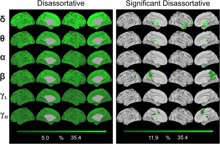
Global mean disassortative community interactions in the frequency domain across participants. (Left panel) spatial distribution of disassortativity overlaid onto the brain. Each row indicates the considered frequency band. The color‐bar is customized between minimum and maximum values within the considered meso‐scale modality. (Right panel) significant nodes according to the community motifs, as revealed by the nonparametric permutation test. Columns and rows as in the left panel. See also Tables S8–S13, for further information about each significant node's name and MNI coordinate, according to the definition given in the AICHA

FIGURE 5.

Global mean core‐periphery community interactions in the frequency domain across participants. (Left panel) Spatial distribution of core‐periphery overlaid onto the brain. Each row indicates the considered frequency band. The color‐bar is customized between minimum and maximum values within the considered meso‐scale modality. (Right panel) Significant nodes according to the community motifs, as revealed by the nonparametric permutation test. Columns and rows as in the left panel. See also Tables S8–S13, for further information about each significant node's name and MNI coordinate, according to the definition given in the AICHA

As for the disassortative structure (Figure 4), significant areas were mostly located in temporal gyrus, insula, and in subcortical areas such as caudate nucleus, putamen, and thalamus for δ band, whereas thalamus and occipital areas for θ band (again, subcortical areas are not depicted, for their description see Table S8 (for δ) and Table S9 (for θ)). Precuneus, posterior cingulate cortex, and parietal areas were instead significant for the β band. It is worth noting that thalamus was significantly disassortative in all bands (with the exception of γ _L, see Tables S8–S13).

Finally, the overall level of core‐periphery motif (Figure 5) was mostly uniform in the whole‐brain, resulting in generally sparse and less significant brain areas than for the other two motifs. Notably, for slow oscillations we found statistically significant core‐peripheriness mostly in the occipital and temporal areas (δ) as well as in the frontal, motor areas and insula (θ).

3.3. Meso‐scale invariants across partitions

We further characterized the meso‐scale structure by looking at invariant modules across partitions. We observed how nodes belonging to the three communities in K = 3 were maintained clustered together or, on the contrary, they were assigned to other partitions from K >3. With this procedure, we identified modules whose brain regions were assigned by the WSBM to the same clusters independently from the number of partitions required to be detected (see alluvial plots in Figure 6). Each transition identified the assignment of each clusters from K = 3 until K = 8 partitions. When nodes were clustered together across partitions, we assigned the same color‐code to the corresponding flow (i.e., light‐red, yellow and dark blue, see Figure 6). Albeit communities reconfigured across K‐values, we highlighted invariant meso‐scale pattern, regardless of the K ^th partition.

FIGURE 6.

Communities reconfiguration across K‐th partitions. Alluvial plots indicating three set of nodes (light‐red, yellow, and dark blue) assigned to the same community regardless of the partitions in each band—δ (a1), θ (a2), α (a3), β (a4), γ _L (a5), and γ _H (a6). Gray flows indicate nodes failing to address the criteria defining main flows across partitions. Every time a colored flow's branch fades toward gray indicates that nodes terminated in a different cluster. Vertical black lines on each side of the transitions indicates originating (from the lower‐grain partition—left side) and arrival clusters (to the adjacent higher‐grain partition—right side)

We further identified those brain areas that belonged to these invariant clusters and, at the same time, showed a maximally significant amount of between‐community interactions (see Figure 6 and Tables S14–S19). Interestingly, different areas across bands addressed these two criteria, and we defined these areas as PGI. Several occipital and temporal areas which showed significant level of core‐peripheriness (see Figure 5), were also found invariant to the number of communities imposed in the δ band (see Figure 7, panel a1 and Table S14). The same held for superior, middle frontal gyrus and precentral sulcus, but for the θ band (see Figure 7, panel a2 and Table S15). Instead, we found that a large portion of left frontal areas in the α band had a significant level of assortativity (see Figure 3) and were assigned to same community across partitions (see Figures 7, panel a3 and Table S16). The β band, unlike the three previous rhythms, exhibited PGI areas in all three community motifs: left frontal areas (assortative), various parietal areas, cingulate and posterior cingulate cortex (PCC), precuneus and thalamus (disassortative), and right inferior frontal areas (core‐periphery) (see Figures 7, panel a4 and Table S17). Both γ _L and γ _H exhibited PGI regions in occipital and temporal areas (assortative), and for γ _H only also in cingulate sulcus and supplementary motor area (disassortative; see Figures 7, panel a5 and a6, and Tables S18 and S19).

FIGURE 7.

Participation and granularity invariant regions. Highlighted areas indicate areas that both belong to an invariant community across partitions and show significant level of assortativity (PGI‐assortative areas, orange), disassortativity (PGI‐disassortative, dark red) and core‐peripheriness (white, PGI‐core‐periphery). Each row indicates a frequency band—δ (a1), θ (a2), α (a3), β (a4), γ _L (a5), γ _H (a6). For a complete description of PGI areas, see also Tables S14–S19 as some subcortical regions are not depicted

In sum, we found PGI‐assortative nodes in frontal areas for α and β rhythms, and in posterior areas, mainly occipital and temporal, for both γ oscillations. PGI‐disassortative nodes was predominant in the cingulate cortex in β and γ _H (also PCC in β band), precuneus and some parietal areas (β). Finally, slow rhythms were characterized by PGI‐core‐peripheriness mostly in the occipital, temporal (δ), and frontal regions (θ), as well as small portion of the right frontal lobe (β).

4. DISCUSSION

To date, the features of human brain meso‐scale structure during resting state have not been fully investigated. Specifically, meso‐scale spectral features are still largely unexplored, and evidence about how the repertoire of community motifs (i.e., assortative, disassortative, and core‐periphery) is associated with different neural oscillations is missing. Thus, we aimed at filling this knowledge gap by using WSBM to infer the diversity of the latent community structure, estimated from source‐reconstructed hdEEG resting state signals. By relying on the spectral richness of hdEEG recordings, we could investigate how FC network meso‐scale is organized across frequency bands. We described the spatial distribution of communities and we characterized their interactions across the frequency domain. According to our results, the meso‐scale is characterized by a frequency‐specific organization. Also, with our experiments and analyses, we highlighted a relevant amount of nonassortative community structure. Additionally, we found that specific brain areas preferably participate in specific community motifs, depending on the oscillatory rhythms. Finally, we identified the so‐called PGI areas exhibiting invariance across partitions and the highest community motif level.

4.1. Meso‐scale structure is frequency‐dependent

We observed an increasing occurrence of the assortative structure when increasing the neuronal oscillation frequency from δ to γ _H, with greater values in the γ _L band. Conversely, the disassortative structure showed an opposite trend, exhibiting highest values in δ and θ slow rhythms. Importantly, communities mostly followed a core‐periphery structure to interact among each other, regardless of the specific frequency band. Indeed, core‐periphery was uniformly distributed across the spectrum, without any particular trend. Given this frequency‐specific organization, we propose in the following that each of the three meso‐scale structure might underlie a particular mechanism of neuronal oscillations.

Slow brain rhythms, are characterized by long‐range communication (Leong et al., 2016; Samogin et al., 2020), and information is exchanged over long‐distance. We suggest that this behavior might be expressed by the disassortative structure which, we found, is higher in δ and θ when compared to the γ _L rhythm, thus favoring integration between long‐distance areas belonging to spatially distinct modules (Betzel, Bertolero, et al., 2018). Therefore, we can consider the disassortative structure as a meso‐scale property of the slow oscillations. Moreover, in δ and θ bands, the WSBM clustering is more fragmented than in the higher frequency bands (lower Calinski–Harabasz index, as reported in Figure S6), likely because these oscillatory regimens are characterized by long‐range interactions (Leong et al., 2016), which might complicate the formation of communities whose brain nodes are spatially closed and/or belong to the same functional domain. This communities' shattering in slow rhythms can be observed at each of the K‐th partition (see Figures 1 and S1–S5) and might further support the hypothesis of central role of disassortativity for slow oscillations.

On the other hand, for higher frequencies (from δ to γ _L and γ _H band) we encountered not only an increase of the assortative meso‐scale structure (with a significant peak in γ _L), but also a clearer subdivision of the communities with respect to the low bands (see Figures 1 and S6) that, in turn, may reflect a local and spatially–segregated processing. In further support of this, there are few branches deviating from the originating community for the high rhythms (see Figure 6), further corroborating the idea that, for fast oscillations, the community detection found more segregated clusters (higher Calinski–Harabasz index, as reported in Figure S6). In fact, gamma‐oscillations might represent a rhythmic synaptic inhibition mediated by parvalbumin‐expressing inhibitory interneurons and the interconnected pyramidal neurons (Buzsaki, Logothetis, & Singer, 2013; Sohal, 2012, 2016). Gamma‐oscillations and the associated assortative structure, might thus resemble a local processing mediated by short‐range connectivity patterns, as also recently demonstrated (Samogin et al., 2020).

Core‐periphery community structure, which is the most represented in all the frequency bands, may underlie the meso‐scale backbone supporting two well‐known strictly interconnected principles of brain organization: local segregation and functional integration (Sporns, 2010). The highly dense core could represent the segregation while the interactions between the core and the nodes located in the peripheries could indicate the presence of functional connections, which might in turn reflect an efficient integration. From this perspective, a plausible interpretation is that the core‐periphery meso‐scale structure might be a good candidate to support this physiological balance between segregation and integration across frequency bands (Sporns, 2010). Previous studies have indeed demonstrated that neuronal oscillations in the gamma band reflect not only a local processing, but may also exhibit synchronization across long‐distance areas (Buzsáki & Schomburg, 2015; Sohal, 2016).

However, all these interpretations have a speculative nature and further EEG studies are needed to potentially validate these claims. Therefore, the meso‐scale structure might be inferred starting from others FC methods, such as phase synchronization (Zhigalov et al., 2017). As an alternative to FC, WSBM works also with directed graph, which can be estimated with hdEEG trough effective connectivity measures (Damborská et al., 2020). Finally, a new method which combines information of FC with structural connectivity from MRI (Glomb et al., 2019a) is promising to increase the quality of the hdEEG source‐reconstructed signals and it has been validated using the Louvain (Blondel, Guillaume, Lambiotte, & Lefebvre, 2008) algorithm which is nevertheless limited to detect assortative community motif.

In summary, we found the emergence of nonassortative meso‐scale structures, by means of noninvasive electrophysiological recordings. According to previous studies focusing on structural and functional MRI, the brain presents a mixed meso‐scale organization, but the network predominantly exhibits modular/assortative meso‐scale structures, specifically during resting state (Betzel, Bertolero, et al., 2018; Betzel, Medaglia, et al., 2018) and, to a lesser extent, during cognitive tasks (Betzel, Bertolero, et al., 2018). Our analysis showed that the amount of assortative modules was reduced when decomposing the time‐course in the frequency domain, and a clear nonassortative organization arose.

4.2. Community motifs rely on brain areas location and frequency band

We further aimed at identifying which brain regions were at the same time insensitive to partitioning and exhibited the highest community motifs in each band (PGI areas). PGI‐assortative areas were located, for γ oscillations, in posterior areas spanning portions of the occipital and temporal lobes, where they potentially resembled the local processing that is peculiar of γ oscillations (see above). Furthermore, some of these posterior areas, were the visual cortices and the inferior temporal lobe, which are components of the visual what/ventral stream, associated with object recognition (Reddy & Kanwisher, 2006). Interestingly, our subjects were fixating a cross in the middle of a computer screen (eyes‐open resting state paradigm). By contrast, some of the PGI‐disassortative areas were located in PCC and angular gyrus (in the β band), which are well‐known areas of the default mode network (DMN) (Marino et al., 2019; Raichle, 2015) and also identified in MEG recordings as cortical hubs (de Pasquale et al., 2018). Albeit the typical oscillatory fingerprint of the DMN is the α rhythm, significant connectivity values between the areas of the DMN, including PCC and angular gyrus, were also found within the β and γ bands (Samogin et al., 2019). Again in the β band, the precuneus showed high disassortativity and this region has been usually associated to self‐referential processing (Cavanna & Trimble, 2006), but it has been also identified as another key area of the DMN, according to fMRI studies (Greicius, Krasnow, Reiss, & Menon, 2003; Utevsky, Smith, & Huettel, 2014). As PCC and angular gyrus, bilateral precuneus is considered a cortical core for β and γ oscillations (Garces et al., 2016). In sum, these areas are cortical cores, which dynamically orchestrate integration of information between networks (de Pasquale et al., 2018). Hence, they may provide a further support of the integrative nature of communities interacting disassortatively (Betzel, Bertolero, et al., 2018).

Frontal areas in α and β showed significant PGI‐assortativity. Some of these frontal areas are part of the dorsal‐lateral prefrontal cortex that is a pivotal area involved in several high‐order executive functions (Barbey, Colom, & Grafman, 2013), such as decision making (Heekeren, Marrett, Ruff, Bandettini, & Ungerleider, 2006) and working memory (Lara & Wallis, 2015), among others (Miller & Cohen, 2001).

Regions showing significant PGI‐core‐peripheriness are instead typical of slow oscillations in frontal lobe (θ) and in occipital and temporal lobes (δ). Particularly, these areas were assortative in higher bands: posterior areas in gamma bands and frontal areas in β. We therefore posit that the same regions might exhibit a community motif depending on the specific neuronal oscillation.

4.3. Study limitations and further development

One possible limitation of our study is that we based our analysis on measurements of spontaneous brain activity, which is brain activity generated in the absence of an explicit task. However, we must recall that many studies about resting state paradigm supported the interpretation that plasticity mechanisms, which depend on previous subjects' interaction with the external world (Carrillo‐Reid, Miller, Hamm, Jackson, & Yuste, 2015; Guerra‐Carrillo, Mackey, & Bunge, 2014; Northoff, 2016), sculpt the activity and bridge together neurons belonging to the same functional domain (motor, visual, auditory, default mode network, among others; Kelly & Castellanos, 2014; Smith et al., 2009; Vincent et al., 2007). Hence, also during spontaneous activity, the co‐activation of these neurons is facilitated and successfully detected by resting state processing pipelines, independently from the noninvasive neuroimaging dataset (Coquelet et al., 2020; Liu et al., 2017). Thus, upon this framework, albeit no specific goal‐directed task is being performed, we can say that the spontaneous activity organization at the meso‐scale level, might largely reflect experience‐dependent plasticity mechanisms, posing the above‐described interpretation as possible candidate of how the brain shapes information flow.

To perform our analysis, we averaged our data in the canonical frequency bands: delta (δ, 1–4 Hz), theta (θ, 4–8 Hz), alpha (α, 8–13 Hz), beta (β, 13–30 Hz), gamma low (γ _L, 30–50 Hz), and gamma high (γ _H, 50–80 Hz; Samogin et al., 2019; Zhao et al., 2019). However, a data‐driven clustering procedure could be used during data processing prior to WSBM application, in order to optimize the frequency bands subdivision and possibly highlight different meso‐scale properties. This is a limitation of our work and it can constitute the starting point for a further exploration of these methodologies in future studies.

As a further improvement, the impact of a different brain atlas on the findings of the present study could be investigated. We selected the AICHA atlas because it is a functionally defined digital atlas of the human brain, developed using resting‐state fMRI connectivity measures (Joliot et al., 2015). However, because a large number of other atlases are defined based on brain structure, we believe that future studies should be conducted to address the role of atlas choice on meso‐scale identification.

An additional observation refers to the number of communities K, which is a free parameter in the context of community detection by WSBM. Here, it has been varied across a range of partitions, allowing for multiple‐grains meso‐scale analysis. This examination showed that each of the frequency band might exhibit its own optimal number of communities. In support of this claim, the flows' reconfiguration in Figure 6 indicates that each band has its own reconfiguration pattern over the partitions, possibly suggesting, in particular for the lower bands, a sub‐optimal fragmentation of modules (when the partition number increases). Moreover, modules fade away and/or remained invariant, depending on the frequency band of interest. Therefore, we suggest that future works should also focus on finding the best K‐granularity per each of the band considered, by performing appropriate parameter selection procedures.

Further expansion of this work should take into account the reproducibility of resting state EEG power spectrum by making use of test–retest validations (Babiloni et al., 2020; Duan et al., 2021). This is especially important when dealing with data from a clinical population.

5. CONCLUSIONS

Our analysis allowed to observe WSBM‐estimated meso‐scale organization with a different focus: by investigating FC in different frequency bands, we captured peculiar features of module interactions revealing the nonassortative nature of resting state networks, demonstrating its frequency‐specificity. Furthermore, this study showed that WSBM applied to sources‐level neuronal oscillations is able to reveal yet unknown properties of FC topological organization.

Overall, these results may be taken into consideration for future studies that will address the pathophysiological mechanisms underlying neurological/psychiatric disorders (Babiloni et al., 2020; Siegel et al., 2012). It would indeed be crucial to examine how the presence of a neurological disease can affect the meso‐scale structure and whether and how a neurorehabilitation intervention can impact the re‐organization of brain networks and the interactions among communities. This will have a direct impact in the clinical assessment of sensory, motor, and cognitive functions, being EEG acquisitions widely employed in the clinical setting. Collectively, the results of our study advance the network neuroscience field by highlighting new features of brain meso‐scale organization.

AUTHOR CONTRIBUTIONS

Riccardo Iandolo, Michela Chiappalone conceived the study. Riccardo Iandolo, Marianna Semprini collected the data. Riccardo Iandolo, Marianna Semprini, Diego Sona, and Michela Chiappalone designed the methods. Riccardo Iandolo, Marianna Semprini performed the analysis. Riccardo Iandolo, Marianna Semprini, Dante Mantin, Laura Avanzino, and Michela Chiappalone interpreted and discussed the results. Riccardo Iandolo, Marianna Semprini, and Michela Chiappalone prepared the figures. Riccardo Iandolo wrote the first version of the manuscript. All the authors contributed to the revision of the manuscript. Part of this work was supported by the Gossweiler foundation, granted to L. Avanzino (PI), D. Mantini, and M. Chiappalone.

Supporting information

Appendix S1: Supporting Information

Iandolo, R., Semprini, M., Sona, D., Mantini, D., Avanzino, L., & Chiappalone, M. (2021). Investigating the spectral features of the brain meso‐scale structure at rest. Human Brain Mapping, 42(15), 5113–5129. 10.1002/hbm.25607

DATA AVAILABILITY STATEMENT

We plan to make the EEG data sets available on Mendeley‐Data repository (or similar). Currently, data are being used for another publication of co‐authors of ours and we cannot share the EEG data at this point.

REFERENCES

- Ahmadlou, M., & Adeli, H. (2011). Functional community analysis of brain: A new approach for EEG‐based investigation of the brain pathology. NeuroImage, 58(2), 401–408. [DOI] [PubMed] [Google Scholar]
- Aicher, C., Jacobs, A. Z., & Clauset, A. (2015). Learning latent block structure in weighted networks. Journal of Complex Networks, 3(2), 221–248. [Google Scholar]
- Babiloni, C., Barry, R. J., Başar, E., Blinowska, K. J., Cichocki, A., Drinkenburg, W. H., … Nunez, P. (2020). International Federation of Clinical Neurophysiology (IFCN)–EEG research workgroup: Recommendations on frequency and topographic analysis of resting state EEG rhythms. Part 1: Applications in clinical research studies. Clinical Neurophysiology, 131(1), 285–307. [DOI] [PubMed] [Google Scholar]
- Barbey, A. K., Colom, R., & Grafman, J. (2013). Dorsolateral prefrontal contributions to human intelligence. Neuropsychologia, 51(7), 1361–1369. 10.1016/j.neuropsychologia.2012.05.017 [DOI] [PMC free article] [PubMed] [Google Scholar]
- Betzel, R. F., & Bassett, D. S. (2017). Multi‐scale brain networks. NeuroImage, 160, 73–83. [DOI] [PMC free article] [PubMed] [Google Scholar]
- Betzel, R. F., Bertolero, M. A., & Bassett, D. S. (2018). Non‐assortative community structure in resting and task‐evoked functional brain networks. bioRxiv, 355016.
- Betzel, R. F., Medaglia, J. D., & Bassett, D. S. (2018). Diversity of meso‐scale architecture in human and non‐human connectomes. Nature Communications, 9(1), 1–14. [DOI] [PMC free article] [PubMed] [Google Scholar]
- Blondel, V. D., Guillaume, J.‐L., Lambiotte, R., & Lefebvre, E. (2008). Fast unfolding of communities in large networks. Journal of Statistical Mechanics: Theory and Experiment, 2008(10), P10008. [Google Scholar]
- Brookes, M. J., Woolrich, M., Luckhoo, H., Price, D., Hale, J. R., Stephenson, M. C., … Morris, P. G. (2011). Investigating the electrophysiological basis of resting state networks using magnetoencephalography. Proceedings of the National Academy of Sciences, 108(40), 16783–16788. [DOI] [PMC free article] [PubMed] [Google Scholar]
- Buzsaki, G., Logothetis, N., & Singer, W. (2013). Scaling brain size, keeping timing: Evolutionary preservation of brain rhythms. Neuron, 80(3), 751–764. 10.1016/j.neuron.2013.10.002 [DOI] [PMC free article] [PubMed] [Google Scholar]
- Buzsáki, G., & Schomburg, E. W. (2015). What does gamma coherence tell us about inter‐regional neural communication? Nature Neuroscience, 18(4), 484–489. [DOI] [PMC free article] [PubMed] [Google Scholar]
- Carrillo‐Reid, L., Miller, J. E., Hamm, J. P., Jackson, J., & Yuste, R. (2015). Endogenous sequential cortical activity evoked by visual stimuli. The Journal of Neuroscience, 35(23), 8813–8828. 10.1523/JNEUROSCI.5214-14.2015 [DOI] [PMC free article] [PubMed] [Google Scholar]
- Cassani, R., Estarellas, M., San‐Martin, R., Fraga, F. J., & Falk, T. H. (2018). Systematic review on resting‐state EEG for Alzheimer's Disease diagnosis and progression assessment. Disease Markers, 2018, 5174815. 10.1155/2018/5174815 [DOI] [PMC free article] [PubMed] [Google Scholar]
- Cavanna, A. E., & Trimble, M. R. (2006). The precuneus: A review of its functional anatomy and behavioural correlates. Brain, 129(Pt 3), 564–583. 10.1093/brain/awl004 [DOI] [PubMed] [Google Scholar]
- Chavez, M., Valencia, M., Navarro, V., Latora, V., & Martinerie, J. (2010). Functional modularity of background activities in normal and epileptic brain networks. Physical Review Letters, 104(11), 118701. 10.1103/PhysRevLett.104.118701 [DOI] [PubMed] [Google Scholar]
- Chen, X., Peng, H., Yu, F., & Wang, K. (2017). Independent vector analysis applied to remove muscle artifacts in EEG data. IEEE Transactions on Instrumentation and Measurement, 66(7), 1770–1779. 10.1109/TIM.2016.2608479 [DOI] [Google Scholar]
- Coito, A., Genetti, M., Pittau, F., Iannotti, G. R., Thomschewski, A., Holler, Y., … Vulliemoz, S. (2016). Altered directed functional connectivity in temporal lobe epilepsy in the absence of interictal spikes: A high density EEG study. Epilepsia, 57(3), 402–411. 10.1111/epi.13308 [DOI] [PubMed] [Google Scholar]
- Coquelet, N., De Tiège, X., Destoky, F., Roshchupkina, L., Bourguignon, M., Goldman, S., … Wens, V. (2020). Comparing MEG and high‐density EEG for intrinsic functional connectivity mapping. NeuroImage, 210, 116556. [DOI] [PubMed] [Google Scholar]
- Crespo‐Garcia, M., Atienza, M., & Cantero, J. L. (2008). Muscle artifact removal from human sleep EEG by using independent component analysis. Annals of Biomedical Engineering, 36(3), 467–475. 10.1007/s10439-008-9442-y [DOI] [PubMed] [Google Scholar]
- Damborská, A., Honzírková, E., Barteček, R., Hořínková, J., Fedorová, S., Ondruš, Š., … Rubega, M. (2020). Altered directed functional connectivity of the right amygdala in depression: High‐density EEG study. Scientific Reports, 10(1), 1–14. [DOI] [PMC free article] [PubMed] [Google Scholar]
- de Pasquale, F., Corbetta, M., Betti, V., & Della Penna, S. (2018). Cortical cores in network dynamics. NeuroImage, 180, 370–382. 10.1016/j.neuroimage.2017.09.063 [DOI] [PubMed] [Google Scholar]
- Duan, W., Chen, X., Wang, Y.‐J., Zhao, W., Yuan, H., & Lei, X. (2021). Reproducibility of power spectrum, functional connectivity and network construction in resting‐state EEG. Journal of Neuroscience Methods, 348, 108985. [DOI] [PubMed] [Google Scholar]
- Faskowitz, J., & Sporns, O. (2020). Mapping the community structure of the rat cerebral cortex with weighted stochastic block modeling. Brain Structure and Function, 225(1), 71–84. [DOI] [PMC free article] [PubMed] [Google Scholar]
- Faskowitz, J., Yan, X., Zuo, X. N., & Sporns, O. (2018). Weighted stochastic block models of the human connectome across the life span. Scientific Reports, 8(1), 12997. 10.1038/s41598-018-31202-1 [DOI] [PMC free article] [PubMed] [Google Scholar]
- Fortunato, S. (2010). Community detection in graphs. Physics Reports‐Review Section of Physics Letters, 486(3–5), 75–174. 10.1016/j.physrep.2009.11.002 [DOI] [Google Scholar]
- Fox, C. W., & Roberts, S. J. (2012). A tutorial on variational Bayesian inference. Artificial Intelligence Review, 38(2), 85–95. [Google Scholar]
- Friston, K. J. (2011). Functional and effective connectivity: A review. Brain Connectivity, 1(1), 13–36. 10.1089/brain.2011.0008 [DOI] [PubMed] [Google Scholar]
- Garces, P., Pereda, E., Hernandez‐Tamames, J. A., Del‐Pozo, F., Maestu, F., & Pineda‐Pardo, J. A. (2016). Multimodal description of whole brain connectivity: A comparison of resting state MEG, fMRI, and DWI. Human Brain Mapping, 37(1), 20–34. 10.1002/hbm.22995 [DOI] [PMC free article] [PubMed] [Google Scholar]
- Garcia, J. O., Ashourvan, A., Muldoon, S. F., Vettel, J. M., & Bassett, D. S. (2018). Applications of community detection techniques to brain graphs: Algorithmic considerations and implications for neural function. Proceedings of the IEEE, 106(5), 846–867. 10.1109/Jproc.2017.2786710 [DOI] [PMC free article] [PubMed] [Google Scholar]
- Glomb, K., Mullier, E., Carboni, M., Rubega, M., Iannotti, G., Tourbier, S., … Hagmann, P. (2019a). Using structural connectivity to augment community structure in EEG functional connectivity. Network Neuroscience, 4(3), 761–787. [DOI] [PMC free article] [PubMed] [Google Scholar]
- Greicius, M. D., Krasnow, B., Reiss, A. L., & Menon, V. (2003). Functional connectivity in the resting brain: A network analysis of the default mode hypothesis. Proceedings of the National Academy of Sciences of the United States of America, 100(1), 253–258. 10.1073/pnas.0135058100 [DOI] [PMC free article] [PubMed] [Google Scholar]
- Guerra‐Carrillo, B., Mackey, A. P., & Bunge, S. A. (2014). Resting‐state fMRI: A window into human brain plasticity. The Neuroscientist, 20(5), 522–533. 10.1177/1073858414524442 [DOI] [PubMed] [Google Scholar]
- Hallquist, M. N., & Hillary, F. G. (2019). Graph theory approaches to functional network organization in brain disorders: A critique for a brave new small‐world. Network neuroscience, 3(1), 1–26. 10.1162/netn_a_00054 [DOI] [PMC free article] [PubMed] [Google Scholar]
- He, B., Sohrabpour, A., Brown, E., & Liu, Z. M. (2018). Electrophysiological source imaging: A noninvasive window to brain dynamics. Annual Review of Biomedical Engineering, 20(20), 171–196. 10.1146/annurev-bioeng-062117-120853 [DOI] [PMC free article] [PubMed] [Google Scholar]
- Heekeren, H. R., Marrett, S., Ruff, D. A., Bandettini, P., & Ungerleider, L. G. (2006). Involvement of human left dorsolateral prefrontal cortex in perceptual decision making is independent of response modality. Proceedings of the National Academy of Sciences, 103(26), 10023–10028. [DOI] [PMC free article] [PubMed] [Google Scholar]
- Hipp, J. F., Hawellek, D. J., Corbetta, M., Siegel, M., & Engel, A. K. (2012). Large‐scale cortical correlation structure of spontaneous oscillatory activity. Nature Neuroscience, 15(6), 884–890. 10.1038/nn.3101 [DOI] [PMC free article] [PubMed] [Google Scholar]
- Huang, L., Wang, C.‐D., & Chao, H. (2019). oComm: Overlapping community detection in multi‐view brain network. IEEE/ACM Transactions on Computational Biology and Bioinformatics. [DOI] [PubMed]
- Iandolo, R., Semprini, M., Buccelli, S., Barban, F., Zhao, M., Samogin, J., … Chiappalone, M. (2020). Small‐world propensity reveals the frequency specificity of resting state networks. IEEE Open Journal of Engineering in Medicine and Biology, 1, 57–64. [DOI] [PMC free article] [PubMed] [Google Scholar]
- Joliot, M., Jobard, G., Naveau, M., Delcroix, N., Petit, L., Zago, L., … Tzourio‐Mazoyer, N. (2015). AICHA: An atlas of intrinsic connectivity of homotopic areas. Journal of Neuroscience Methods, 254, 46–59. 10.1016/j.jneumeth.2015.07.013 [DOI] [PubMed] [Google Scholar]
- Kabbara, A., Falou, W. E., Khalil, M., Wendling, F., & Hassan, M. (2017). The dynamic functional core network of the human brain at rest. Scientific Reports, 7(1), 1–16. [DOI] [PMC free article] [PubMed] [Google Scholar]
- Kane, N., Acharya, J., Benickzy, S., Caboclo, L., Finnigan, S., Kaplan, P. W., … van Putten, M. (2017). A revised glossary of terms most commonly used by clinical electroencephalographers and updated proposal for the report format of the EEG findings. Revision 2017. Clinical Neurophysiology Practice, 2, 170–185. 10.1016/j.cnp.2017.07.002 [DOI] [PMC free article] [PubMed] [Google Scholar]
- Kelly, C., & Castellanos, F. X. (2014). Strengthening connections: Functional connectivity and brain plasticity. Neuropsychology Review, 24(1), 63–76. 10.1007/s11065-014-9252-y [DOI] [PMC free article] [PubMed] [Google Scholar]
- Lara, A. H., & Wallis, J. D. (2015). The role of prefrontal cortex in working memory: A mini review. Frontiers in Systems Neuroscience, 9, 173. 10.3389/fnsys.2015.00173 [DOI] [PMC free article] [PubMed] [Google Scholar]
- Leong, A. T., Chan, R. W., Gao, P. P., Chan, Y. S., Tsia, K. K., Yung, W. H., & Wu, E. X. (2016). Long‐range projections coordinate distributed brain‐wide neural activity with a specific spatiotemporal profile. Proceedings of the National Academy of Sciences of the United States of America, 113(51), E8306–E8315. 10.1073/pnas.1616361113 [DOI] [PMC free article] [PubMed] [Google Scholar]
- Liu, Y., Balsters, J. H., Baechinger, M., van der Groen, O., Wenderoth, N., & Mantini, D. (2015). Estimating a neutral reference for electroencephalographic recordings: The importance of using a high‐density montage and a realistic head model. Journal of Neural Engineering, 12(5), 056012. [DOI] [PMC free article] [PubMed] [Google Scholar]
- Liu, Y., Farahibozorg, S., Porcaro, C., Wenderoth, N., & Mantini, D. (2017). Detecting large‐scale networks in the human brain using high‐density electroencephalography. Human Brain Mapping, 38(9), 4631–4643. 10.1002/hbm.23688 [DOI] [PMC free article] [PubMed] [Google Scholar]
- Marino, M., Arcara, G., Porcaro, C., & Mantini, D. (2019). Hemodynamic correlates of electrophysiological activity in the default mode network. Frontiers in Neuroscience, 13, 1060. 10.3389/fnins.2019.01060 [DOI] [PMC free article] [PubMed] [Google Scholar]
- Marzetti, L., Della Penna, S., Snyder, A. Z., Pizzella, V., Nolte, G., De Pasquale, F., … Corbetta, M. (2013). Frequency specific interactions of MEG resting state activity within and across brain networks as revealed by the multivariate interaction measure. NeuroImage, 79, 172–183. [DOI] [PMC free article] [PubMed] [Google Scholar]
- Miller, E. K., & Cohen, J. D. (2001). An integrative theory of prefrontal cortex function. Annual Review of Neuroscience, 24, 167–202. 10.1146/annurev.neuro.24.1.167 [DOI] [PubMed] [Google Scholar]
- Newman, M. E. J. (2006). Modularity and community structure in networks. Proceedings of the National Academy of Sciences of the United States of America, 103(23), 8577–8582. 10.1073/pnas.0601602103 [DOI] [PMC free article] [PubMed] [Google Scholar]
- Northoff, G. (2016). Neuro‐philosophy and the healthy mind: Learning from the unwell brain. New York, NY: WW Norton & Company. [Google Scholar]
- Oldfield, R. C. (1971). The assessment and analysis of handedness: The Edinburgh inventory. Neuropsychologia, 9(1), 97–113. 10.1016/0028-3932(71)90067-4 [DOI] [PubMed] [Google Scholar]
- Pascual‐Marqui, R. D., Lehmann, D., Koukkou, M., Kochi, K., Anderer, P., Saletu, B., … Kinoshita, T. (2011). Assessing interactions in the brain with exact low‐resolution electromagnetic tomography. Philosophical Transactions of The Royal Society A Mathematical Physical and Engineering Sciences, 369(1952), 3768–3784. 10.1098/rsta.2011.0081 [DOI] [PubMed] [Google Scholar]
- Pavlovic, D. M., Vertes, P. E., Bullmore, E. T., Schafer, W. R., & Nichols, T. E. (2014). Stochastic blockmodeling of the modules and core of the Caenorhabditis elegans connectome. PLoS One, 9(7), e97584. 10.1371/journal.pone.0097584 [DOI] [PMC free article] [PubMed] [Google Scholar]
- Puxeddu, M., Petti, M., Mattia, D., & Astolfi, L. (2019). The optimal setting for multilayer modularity optimization in multilayer brain networks. Paper Presented at the 2019 41st Annual International Conference of the IEEE Engineering in Medicine and Biology Society (EMBC). [DOI] [PubMed]
- Puxeddu, M., Petti, M., Pichiorri, F., Cincotti, F., Mattia, D., & Astolfi, L. (2017). Community detection: Comparison among clustering algorithms and application to EEG‐based brain networks. Paper presented at the 2017 39th Annual International Conference of the IEEE Engineering in Medicine and Biology Society (EMBC). [DOI] [PubMed]
- Raichle, M. E. (2015). The brain's default mode network. Annual Review of Neuroscience, 38(38), 433–447. 10.1146/annurev-neuro-071013-014030 [DOI] [PubMed] [Google Scholar]
- Reddy, L., & Kanwisher, N. (2006). Coding of visual objects in the ventral stream. Current Opinion in Neurobiology, 16(4), 408–414. 10.1016/j.conb.2006.06.004 [DOI] [PubMed] [Google Scholar]
- Reid, A. T., Headley, D. B., Mill, R. D., Sanchez‐Romero, R., Uddin, L. Q., Marinazzo, D., … Cole, M. W. (2019). Advancing functional connectivity research from association to causation. Nature Neuroscience, 22(11), 1751–1760. 10.1038/s41593-019-0510-4 [DOI] [PMC free article] [PubMed] [Google Scholar]
- Rubinov, M., & Sporns, O. (2010). Complex network measures of brain connectivity: Uses and interpretations. NeuroImage, 52(3), 1059–1069. 10.1016/j.neuroimage.2009.10.003 [DOI] [PubMed] [Google Scholar]
- Samogin, J., Liu, Q., Marino, M., Wenderoth, N., & Mantini, D. (2019). Shared and connection‐specific intrinsic interactions in the default mode network. NeuroImage, 200, 474–481. [DOI] [PubMed] [Google Scholar]
- Samogin, J., Marino, M., Porcaro, C., Wenderoth, N., Dupont, P., Swinnen, S. P., & Mantini, D. (2020). Frequency‐dependent functional connectivity in resting state networks. Human Brain Mapping, 41(18), 5187–5198. [DOI] [PMC free article] [PubMed] [Google Scholar]
- Seeber, M., Cantonas, L. M., Hoevels, M., Sesia, T., Visser‐Vandewalle, V., & Michel, C. M. (2019). Subcortical electrophysiological activity is detectable with high‐density EEG source imaging. Nature Communications, 10, 753. [DOI] [PMC free article] [PubMed] [Google Scholar]
- Siegel, M., Donner, T. H., & Engel, A. K. (2012). Spectral fingerprints of large‐scale neuronal interactions. Nature Reviews. Neuroscience, 13(2), 121–134. 10.1038/nrn3137 [DOI] [PubMed] [Google Scholar]
- Siems, M., Pape, A. A., Hipp, J. F., & Siegel, M. (2016). Measuring the cortical correlation structure of spontaneous oscillatory activity with EEG and MEG. NeuroImage, 129, 345–355. 10.1016/j.neuroimage.2016.01.055 [DOI] [PubMed] [Google Scholar]
- Siems, M., & Siegel, M. (2020). Dissociated neuronal phase‐ and amplitude‐coupling patterns in the human brain. NeuroImage, 209, 116538. 10.1016/j.neuroimage.2020.116538 [DOI] [PMC free article] [PubMed] [Google Scholar]
- Smith, S. M., Fox, P. T., Miller, K. L., Glahn, D. C., Fox, P. M., Mackay, C. E., … Beckmann, C. F. (2009). Correspondence of the brain's functional architecture during activation and rest. Proceedings of the National Academy of Sciences of the United States of America, 106(31), 13040–13045. 10.1073/pnas.0905267106 [DOI] [PMC free article] [PubMed] [Google Scholar]
- Sohal, V. S. (2012). Insights into cortical oscillations arising from optogenetic studies. Biological Psychiatry, 71(12), 1039–1045. [DOI] [PMC free article] [PubMed] [Google Scholar]
- Sohal, V. S. (2016). How close are we to understanding what (if anything) γ oscillations do in cortical circuits? Journal of Neuroscience, 36(41), 10489–10495. [DOI] [PMC free article] [PubMed] [Google Scholar]
- Sporns . (2010). Networks of the brain. Cambridge, MA: MIT Press. [Google Scholar]
- Sporns . (2018). Graph theory methods: Applications in brain networks. Dialogues in Clinical Neuroscience, 20(2), 111–121. [DOI] [PMC free article] [PubMed] [Google Scholar]
- Taberna, G. A., Guarnieri, R., & Mantini, D. (2019). SPOT3D: Spatial positioning toolbox for head markers using 3D scans. Scientific Reports, 9(1), 1–9. [DOI] [PMC free article] [PubMed] [Google Scholar]
- Uriguen, J. A., & Garcia‐Zapirain, B. (2015). EEG artifact removal‐state‐of‐the‐art and guidelines. Journal of Neural Engineering, 12(3), 031001. 10.1088/1741-2560/12/3/031001 [DOI] [PubMed] [Google Scholar]
- Utevsky, A. V., Smith, D. V., & Huettel, S. A. (2014). Precuneus is a functional core of the default‐mode network. Journal of Neuroscience, 34(3), 932–940. [DOI] [PMC free article] [PubMed] [Google Scholar]
- Vidaurre, D., Hunt, L. T., Quinn, A. J., Hunt, B. A., Brookes, M. J., Nobre, A. C., & Woolrich, M. W. (2018). Spontaneous cortical activity transiently organises into frequency specific phase‐coupling networks. Nature Communications, 9(1), 1–13. [DOI] [PMC free article] [PubMed] [Google Scholar]
- Vincent, J. L., Patel, G. H., Fox, M. D., Snyder, A. Z., Baker, J. T., Van Essen, D. C., … Raichle, M. E. (2007). Intrinsic functional architecture in the anaesthetized monkey brain. Nature, 447(7140), 83–86. 10.1038/nature05758 [DOI] [PubMed] [Google Scholar]
- Waninger, S., Berka, C., Stevanovic Karic, M., Korszen, S., Mozley, P. D., Henchcliffe, C., … Verma, A. (2020). Neurophysiological biomarkers of Parkinson's Disease. Journal of Parkinson's Disease, 10, 1–10. [DOI] [PMC free article] [PubMed] [Google Scholar]
- Zhao, M., Marino, M., Samogin, J., Swinnen, S. P., & Mantini, D. (2019). Hand, foot and lip representations in primary sensorimotor cortex: A high‐density electroencephalography study. Scientific Reports, 9(1), 19464. 10.1038/s41598-019-55369-3 [DOI] [PMC free article] [PubMed] [Google Scholar]
- Zhigalov, A., Arnulfo, G., Nobili, L., Palva, S., & Palva, J. M. (2017). Modular co‐organization of functional connectivity and scale‐free dynamics in the human brain. Network Neuroscience, 1(2), 143–165. 10.1162/NETN_a_00008 [DOI] [PMC free article] [PubMed] [Google Scholar]
Associated Data
This section collects any data citations, data availability statements, or supplementary materials included in this article.
Supplementary Materials