DEER spectroscopy can be used to investigate the conformational equilibria of proteins. In this tutorial, we illustrate the rigorous global analysis of DEER data to quantitively analyze these equilibria to determine the populations of distinct intermediates under varying biochemical conditions.
Abstract
The potential of spin labeling to reveal the dynamic dimension of macromolecules has been recognized since the dawn of the methodology in the 1960s. However, it was the development of pulsed electron paramagnetic resonance spectroscopy to detect dipolar coupling between spin labels and the availability of turnkey instrumentation in the 21st century that realized the full promise of spin labeling. Double electron-electron resonance (DEER) spectroscopy has seen widespread applications to channels, transporters, and receptors. In these studies, distance distributions between pairs of spin labels obtained under different biochemical conditions report the conformational states of macromolecules, illuminating the key movements underlying biological function. These experimental studies have spurred the development of methods for the rigorous analysis of DEER spectroscopic data along with methods for integrating these distributions into structural models. In this tutorial, we describe a model-based approach to obtaining a minimum set of components of the distance distribution that correspond to functionally relevant protein conformations with a set of fractional amplitudes that define the equilibrium between these conformations. Importantly, we review and elaborate on the error analysis reflecting the uncertainty in the various parameters, a critical step in rigorous structural interpretation of the spectroscopic data.
Introduction
The modern tool kit of structural biology includes diverse, complementary methods spanning the spectrum from computational to experimental that can visualize global structures at atomic resolution as well as probe them on local site-specific levels and can reveal the dynamic dimension under equilibrium or time-resolved conditions. The integration of these methods has been touted as the next frontier in the quest to reveal the interplay of structure and dynamics that underpins protein function. Probe methods, including electron paramagnetic resonance (EPR) spectroscopy of site-specifically spin-labeled proteins, have contributed a unique perspective on protein dynamics (Mchaourab et al., 2011; Claxton et al., 2015; Jeschke, 2018a). In particular, pulsed EPR methods are distinguished by the ability to investigate proteins in multiple conformational states in near-native environments with high sensitivity. Because integration of structural biology data is mostly performed a posteriori, the process requires not only knowledge of the rules of interpretation (i.e., how models are derived from data) but also well-established tools for assessment of rigor and reproducibility of the underlying analysis.
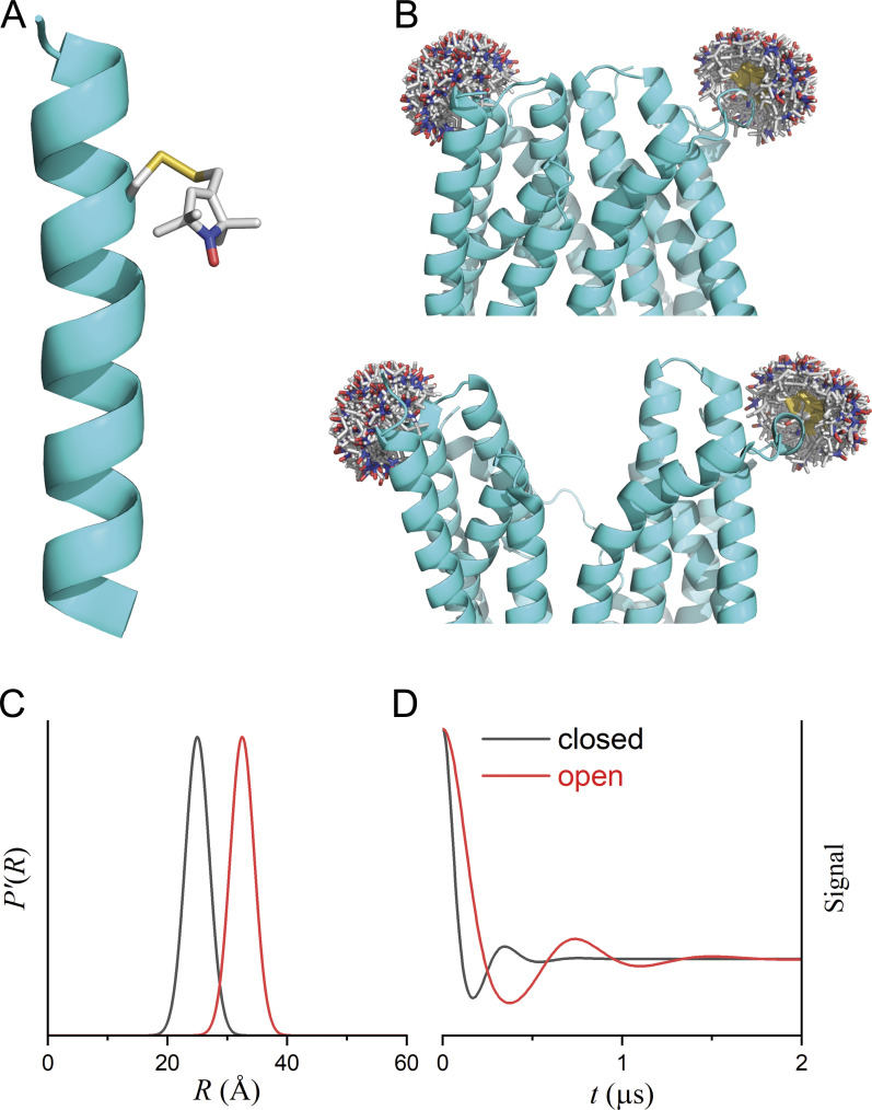
The pulsed EPR technique double electron-electron resonance (DEER) spectroscopy measures long-range (>20 Å) distances between electron spins (Jeschke, 2012; Borbat and Freed, 2014; Jeschke, 2014), typically extrinsic probes introduced into biological macromolecules by site-directed spin labeling (Roser et al., 2016). DEER has been applied to multiple proteins, RNA, and DNA systems. In the protein space, unique insight was revealed on ion channel architecture and gating (Pliotas et al., 2012; Dellisanti et al., 2013; Dalmas et al., 2014; Dürr et al., 2014; Puljung et al., 2014; Raghuraman et al., 2014; Arrigoni et al., 2016; Zhu et al., 2016; Evans et al., 2020), transporter alternating access and energy landscapes (Claxton et al., 2010; Mittal et al., 2012; Georgieva et al., 2013; Kazmier et al., 2014a; Kazmier et al., 2014b; Masureel et al., 2014; Joseph et al., 2015; Dastvan et al., 2016; Martens et al., 2016; Timachi et al., 2017; Verhalen et al., 2017; Göddeke et al., 2018; Dastvan et al., 2019; Joseph et al., 2019; Nyenhuis et al., 2020), and receptor activation and allosteric modulation (Park et al., 2006; Kim et al., 2012; Kang et al., 2015; Yee et al., 2015; Van Eps et al., 2017; Van Eps et al., 2018; Wingler et al., 2019; Elgeti and Hubbell, 2021). The range of applications of DEER include evaluation of static structures in solution (e.g., Zhou et al., 2005) or native-like environments (e.g., Barrett et al., 2012), probing ligand-induced conformational changes, characterization of equilibrium fluctuations, and investigation of protein–protein interactions (Hilger et al., 2005; Hilger et al., 2007; Kim et al., 2011; Edwards et al., 2014). The most frequent strategy is to attach pairs of spin labels at introduced cysteines in a purified protein (Fig. 1 A), although promising alternative strategies have been introduced (Roser et al., 2016; Ackermann et al., 2021; Gamble Jarvi et al., 2021). Multiple pairs are designed to provide a pattern of characteristic distances or distance changes relevant to the structure or model to be tested. Distance restraints from DEER have been integrated with computation methods to model protein structures ab initio (Alexander et al., 2008; Alexander et al., 2013; Jeschke, 2016), to refine structures, and to generate models of intermediate states (Kazmier et al., 2014b; Evans et al., 2020) or protein complexes (Kim et al., 2012; Edwards et al., 2014). In combination with cryo-EM, DEER distance distributions can provide a complementary approach to pinpoint the mechanistic identity of various conformations and to validate models of conformational changes (Dürr et al., 2014; Zhu et al., 2016).
Figure 1.
Site-directed spin labeling and DEER. (A) Model showing the MTSSL attached to an α-helix at a cysteine residue. (B) Models showing spin labels at extracellular sites of two helices of an integral membrane protein in two different conformational states. (C) The expected distance distributions for the OO (red) and OC (black) states. (D) The corresponding intramolecular DEER signals.
The cornerstones of DEER data interpretation are the rigorous transformation of the raw signals into complex distance distributions, the structural interpretation of these distributions as spatial restraints, and the generation of structural models consistent with the derived restraints. As an illustration, consider a hypothetical membrane transporter doubly labeled at the extracellular surface of two transmembrane (TM) helices (Fig. 1 B) with two conformations, outward closed (OC) and outward open (OO), that differ by a large translocation of one helix relative to the other. The distribution, P, of distances, R, between the labels for each conformation (Fig. 1 C) is determined by its tertiary structures, the degree of disorder in the structure, and the rotameric disorder of the labels. The different distance distributions for the two conformations produce distinct DEER time traces (Fig. 1 D).
More generally, distinct distance components with varying widths in the P(R) reflect the collection of conformations of the protein backbone that are populated under the experimental conditions and the rotameric states of the spin-label side chain at each of these conformations. Biochemical conditions can be manipulated to shift the energies of protein conformers, leading to a set of DEER signal traces that differ by the populations of these components. Here, we focus on tools for the rigorous analysis of multiple DEER time traces obtained under varying conditions from one or more doubly spin-labeled mutants of a given protein. We describe a model-based approach to obtaining a minimum set of distance components related to functionally relevant conformations with a set of fractional amplitudes that define the equilibrium between these conformations together with error analysis reflecting the uncertainty in the various parameters.
From DEER signal to distance distribution
Much work has been devoted to the development of methods for the analysis of DEER data to determine the optimal P(R). Broadly, these methods can be described as either model based, expressing the P(R) as a linear combination of components (typically Gaussian), or model free, often using a mathematical regularization method. A DEER time-domain experimental signal, V(t), is the product of a signal, VO(t), arising from the dipolar interactions within a labeled molecule or complex and a background signal, VB(t), arising from intermolecular dipolar interactions (Pannier et al., 2000b; Bowman et al., 2004).
| (1) |
where is random noise drawn from a normal distribution whose variance is independent of t (Edwards and Stoll, 2016). Typically, nitroxide spin labels are sufficiently disordered (see Fig. 1 B) to eliminate correlation between the interspin distance and relative orientation eliminating any orientation selection effects (Polyhach et al., 2007; Schiemann et al., 2009). After averaging over all possible relative orientations, the intramolecular signal, which is the signal of interest, can be modeled as follows:
| (2) |
The modulation depth, Δ, is a function of both the labeling efficiency and various instrumental factors. has been previously defined (Milov et al., 1998; Bowman et al., 2004; Edwards and Stoll, 2016):
| (3) |
where C and S are the Fresnel cosine and sine integrals
| (4) |
and the symbols in the equation for the dipolar frequency, represent the usual physical constants.
The background factor can be modeled as an exponential, a stretched exponential function (Milov et al., 1998),
| (5) |
or any other desired model including one that accounts for an excluded volume effect (Brandon et al., 2012; Kattnig et al., 2013). All data in this work has been fit with a pure exponential background factor (d = 3) corresponding to a 3-D homogeneous solution. The use of an exponential expression, to parameterize the background decay rate reduces the dynamic range of the fit parameter and can improve fitting. For a homogeneous 3-D solution of spins (d = 3), an effective spin concentration can be calculated from the background decay rate (see Appendix).
Model-based analysis of DEER data assumes that P(R) can be described by a sum of n components:
| (6) |
When using Gaussians, the components are given by
| (7) |
However, non-Gaussian basis functions may also be used (Hustedt et al., 2018). For a given model, the best-fit values of each of the parameters are those that minimize the reduced χ2 value:
| (8) |
where Vi is the experimentally measured signal at the ith time point, Oi and are the calculated intramolecular and background signals, is the estimated noise variance, N is the total number of data points, and q is the total number of parameters considered in the fit. The use of a mathematical model to define P(R), specifically the use of a Gaussian basis set, was originally used by Spiess and coworkers (Pannier et al., 2000a), then by Fajer and coworkers (Sen et al., 2007), and has been further developed by us (Brandon et al., 2012; Stein et al., 2015; Hustedt et al., 2018).
Previously, we introduced the Akaike information criterion corrected for finite sample size (AICc; Stein et al., 2015) and the Bayesian information criterion (BIC; Hustedt et al., 2018) for selecting an optimal model from a set used to analyze single DEER datasets based on the principle of parsimony. The set of models considered can test different n values, different basis functions, or differing background decay functions.
| (9) |
| (10) |
These criteria balance the decrease in the sum of squared residuals (SSR) versus the increase in the number of free parameters, q, that comes with increasing model complexity. When selecting from a group of models that have been tested, that with the lowest criterion value can be considered to be the optimal balance of these two factors (Burnham and Anderson, 2002). In practice, we find that the use of BIC is favored over AICc because the former favors more parsimonious models.
The magnitude of the BIC values do not directly reflect the merit of a particular model and cannot be used to determine that a particular model is correct. Their relative values are, however, significant. Setting BIC0 equal to the lowest BIC value of the set, different models can be compared by calculating values.
| (11) |
These values do reflect the relative merit of different models. Rules of thumb have been developed for interpreting ΔBIC values (Raftery, 1995; Burnham and Anderson, 2002). If the ΔBIC value for a particular model from a set under consideration is >10, then the evidence against that model is very strong, and if <2, it is weak. The use of BIC over AICc or any other criterion for model selection is subjective. Additional considerations, if properly justified, can be used to select an appropriate model.
Other approaches to the analysis of DEER data include the commonly used Tikhonov regularization (Chiang et al., 2005; Jeschke et al., 2006; Ibáñez and Jeschke, 2020; Ibáñez et al., 2020), alternative regularization approaches (Ibáñez and Jeschke, 2019), denoising methods followed by singular value decomposition (Srivastava and Freed, 2017; Srivastava et al., 2017; Srivastava and Freed, 2019), and neural networks (Worswick et al., 2018; Amey et al., 2021).
Model-based analysis of DEER data
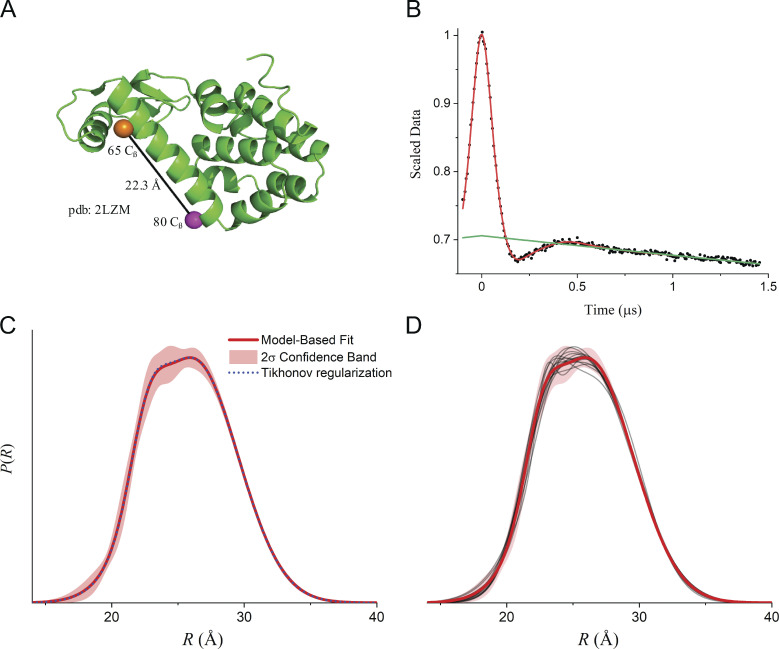
The model-based approach to the analysis of DEER data is illustrated in Fig. 2 using data from T4 lysozyme (T4L) labeled at residues 65 and 80 with the methanethiosulfonate spin label (MTSSL). After a trivial scaling and shift of the time axis, the DEER data are fit using a model-based approach that includes the best-fit background factor. The optimal fit, according to BIC values, models P(R) as a sum of two Gaussians. Table 1 gives the statistics obtained from fitting the data in Fig. 2 to n = 1, 2, and 3 Gaussian components. The BIC values for the n = 1 and n = 3 models both differ from that of the n = 2 model by <10, suggesting that none of these models can be strongly rejected based on this dataset. In fact, the n = 3 model is preferred according to the AICc values. The small amplitude of the third component and the large uncertainty of this amplitude (0.02 ± 0.06), together with the very narrow width of this Gaussian (0.04 ± 2.81 Å), all support the rejection of this more complex model (see Table 2).
Figure 2.
Q-band DEER data and fit for T4L spin-labeled with MTSSL at residues 65 and 80. (A) The crystal structure of T4L (PDB accession no. 2LZM; Matsumura et al., 1989) showing the location of the two spin labels. pdb, Protein Data Bank. (B) The scaled DEER data are shown as filled black circles together with the best model-based fit (red line) and background factor (green line). (C) The best-fit P(R) modeled as the sum of two Gaussians is shown as a red line with the associated 2σ (95%) confidence band as a shaded region. The model-free P(R) obtained using Tikhonov regularization in DeerAnalysis 2019 is also shown (dotted blue line). The optimal regularization factor was determined by generalized cross-validation and the starting time point for background fitting using the validation tool. (D) The solid red line and shaded region duplicate those shown in C. The best-fit P(R) modeled as the sum of 2 Gaussians obtained from 15 replicate datasets are shown as thin black lines.
Table 1. Model statistics from fitting of T4L 65/80 data in Fig. 2.
| n | q | SSR | AICc | BIC | ΔAICc | ΔBIC | |
|---|---|---|---|---|---|---|---|
| 1 | 5 | 0.001984 | 1.0803 | −3,051.3 | −3,030.3 | 17.5 | 5.4 |
| 2 | 8 | 0.001823 | 1.0042 | −3,067.0 | −3,035.7 | 1.8 | 0 |
| 3 | 11 | 0.001765 | 0.9842 | −3,068.8 | −3,027.3 | 0 | 8.3 |
Table 2. Fit parameters for T4L 65/80 data in Fig. 2.
| n | 1 | 2 | 3 |
|---|---|---|---|
| Δ | 0.298 ± 0.002 | 0.297 ± 0.002 | 0.30 ± 0.02 |
| η | 4.61 ± 0.01 | 4.61 ± 0.01 | 4.61 ± 0.01 |
| Scale | 1.003 ± 0.002 | 1.001 ± 0.002 | 1.00 ± 0.03 |
| r 0 | 25.73 ± 0.06 | 22.8 ± 0.5 | 29 ± 4 |
| σR | 3.55 ± 0.08 | 1.3 ± 0.8 | 0.04 ± 2.81 |
| Fraction | 0.10 ± 0.09 | 0.02 ± 0.06 | |
| r 0 | 26.2 ± 0.4 | 26.1 ± 0.6 | |
| σR | 3.4 ± 0.2 | 3.5 ± 0.2 | |
| Fraction | 0.90 ± 0.09 | 0.86 ± 0.16 | |
| r 0 | 23.1 ± 0.7 | ||
| σR | 1.6 ± 1.0 | ||
| Fraction | 0.12 ± 0.16 |
The second component in the optimal P(R) does not give rise to a distinct second mode and is fully consistent with a single backbone conformation of T4L with some inherent disorder and a distribution of rotameric states of the two labels. In other cases discussed below, individual well-separated Gaussian components clearly correspond to distinct backbone conformations. A general rule of thumb is that the number of conformations is less than or equal to the number of Gaussian components.
As has been previously discussed (Hustedt et al., 2018), model-based analysis allows for rigorous error analysis of the best-fit parameter values and the calculation of a confidence band for the best-fit distance distribution from the full covariance matrix using propagation of errors. The 2σ (95%) confidence band for the best-fit n = 2 Gaussian P(R) is shown in Fig. 2 C as a shaded region and reproduced in Fig. 2 D along with the best-fit P(R) for 15 replicate datasets collected for the same sample. These results demonstrate that the confidence band obtained from fitting a given dataset properly estimates the reproducibility of the distance distribution.
The P(R) obtained using Tikhonov regularization is also shown in Fig. 2 C. The model-free P(R) is quite close to the P(R) modeled as the sum of two Gaussians. Both the model-based approach as developed primarily at Vanderbilt University (Brandon et al., 2012; Stein et al., 2015; Hustedt et al., 2018) and the model-free approach using Tikhonov regularization, as developed primarily by Jeschke et al. (2006), have been extensively used to analyze DEER data and are well documented. Although historically the use of Tikhonov regularization to give model-free fits to DEER data has required an initial background correction step, recently an approach for applying Tikhonov regularization to uncorrected data has been developed (Ibáñez and Jeschke, 2020; Ibáñez et al., 2020).
Videos demonstrating the use of either DD (Video 1) or GLADDvu (Video 2) to perform the model-based fits of this T4L dataset are available online. DD and GLADDvu are available for download at https://github.com/erichustedt/.
Video 1.
Demonstration of the use of DD (https://github.com/erichustedt/DD) to perform the model-based fits of a T4L dataset. The fits listed in Table 1 and Table 2 using n = 1, 2, and 3 Gaussians are perforrmed using DD. The optimal results, as determined by BIC values, were obtained for n = 2 and are shown in Fig. 2. The dataset (T4L065-080M_08) is available for dowload.
Video 2.
Demonstration of the use of GLADDvu (https://github.com/erichustedt/GLADDvu) to perform the model-based fits of a T4L dataset. The fits listed in Table 1 and Table 2 using n = 1, 2, and 3 Gaussians are perforrmed using GLADDvu. The optimal results, as determined by BIC values, were obtained for n = 2 and are shown in Fig. 2. The dataset (T4L065-080M_08) is available for dowload.
Global analysis paradigm
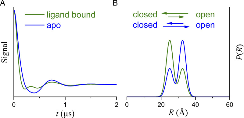
A set of DEER experiments collected under different experimental conditions can contain information far beyond what can be inferred from the collection of P(R) obtained from individual fits to the traces. In Fig. 1 B, each conformation leads to an interlabel distance distribution that can be modeled as a single Gaussian component whose width is determined by the distribution of rotameric states of the labels. In practice, conditions may not be available that would allow the collection of data corresponding to the pure OO or OC conformations. Instead, different conditions, here ligand bound and ligand free (apo), favor the OC and OO conformations, respectively (Fig. 3 A). Qualitatively, the data and the P(R) are consistent with a shift in the equilibrium from one favoring OO to OC upon ligand binding.
| (12) |
where and are the fractions of apo and ligand-bound transporter in the OO state. Likewise, and are the interspin distance distributions of the pure OC and OO states.
Figure 3.
DEER data assuming that two conformations are in equilibrium. (A) Simulated DEER data assuming that ligand binding (green line) favors the OC state. (B) The corresponding P(R).
More generally, the P(R) for condition can be expressed as a common set of corresponding to different conformations.
| (13) |
A more pertinent analysis of the data in Fig. 3 B would allow one to recover estimates of the distance distributions, for structural modeling of the pure conformational states and the set of coefficients, for defining equilibrium constants and other thermodynamic parameters. This tutorial focuses on the linked fitting of the datasets (i.e., the global analysis of multiple DEER time traces) to obtain this full description of the system under investigation using models that explicitly link the conformations under different conditions.
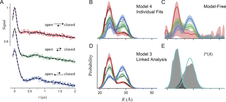
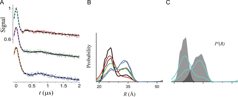
To demonstrate putting these concepts into practice, consider the three simulated DEER traces in Fig. 4 that were calculated for bimodal P(R) generated from the same two unimodal distributions selected from the test set generated by Edwards and Stoll (2018) with different relative amplitudes (Table 3). The underlying biological model is that the protein is undergoing a ligand-dependent shift in the equilibrium between two conformational states. Given the P(R) obtained from fitting these data individually, either to bimodal Gaussian distributions (Fig. 4 B) or using a Tikhonov regularization (Fig. 4 C), it would be hard to argue convincingly whether the protein is or is not behaving according to this model of its functional dynamics (i.e., that the protein adopts the same two conformational states at all ligand concentrations albeit in different proportions).
Figure 4.
Global analysis of simulated DEER data. (A) The data (filled circles) were simulated for P(R) modeled as the sum of two components using the amplitudes in Table 3. The true P'(R) of the components are distributions 5347 and 483 from the set of distributions calculated by Edwards and Stoll (2018) using MMM (Jeschke, 2018b) for T4L labeled at 118/154 and 8/126 with means/SDs of 25.1/1.9 Å and 32.6/3.0 Å, respectively. The best-fit lines for model 3 (R0 and σR values linked) and model 4 (no parameters linked) are shown as solid black and dashed colored lines, respectively. (B) P(R) for model 4 for datasets A (red), B (green), and C (blue) with the associated 2σ (95%) confidence bands as shaded regions. The black lines are the true P(R) used for the simulations. (C) Best-fit P(R) from Tikhonov regularization using DeerLab version 0.13.2 using the same color scheme. The optimal regularization factor was determined by generalized cross-validation. (D) Best-fit P(R) for model 3 using the same color scheme with the associated 2σ (95%) confidence bands as the shaded regions. The black lines are the true P(R) used for the simulations. (E) The P'(R) obtained for model 3 is shown in cyan, and the true P'(R) used for the simulations is superimposed as shaded regions. Both the x and y axis scales are the same for B–E.
Table 3. Fit parameters for simulated data in Fig. 4.
| Data set | A | B | C | ||||
|---|---|---|---|---|---|---|---|
| Simulation | Fraction | 0.75 | 0.25 | 0.5 | 0.5 | 0.25 | 0.75 |
| Fit to model 3: linked analysis | r 0 | 25.4 ± 0.3 | 33.0 ± 0.4 | 25.4 ± 0.3 | 33.0 ± 0.4 | 25.4 ± 0.3 | 33.0 ± 0.4 |
| σ r | 2.0 ± 0.3 | 2.6 ± 0.4 | 2.0 ± 0.3 | 2.6 ± 0.4 | 2.0 ± 0.3 | 2.6 ± 0.4 | |
| Fraction | 0.20 ± 0.04 | 0.46 ± 0.05 | 0.70 ± 0.06 | ||||
| Fit to model 4: individual fits | r 0 | 25.2 ± 0.4 | 32.8 ± 3.1 | 26.2 ± 0.9 | 33.7 ± 1.1 | 25.6 ± 0.7 | 33.1 ± 0.5 |
| σ r | 1.9 ± 0.4 | 3.4 ± 2.6 | 2.6 ± 0.9 | 2.1 ± 0.9 | 1.6 ± 0.7 | 2.6 ± 0.5 | |
| Fraction | 0.24 ± 0.15 | 0.36 ± 0.14 | 0.70 ± 0.07 | ||||
However, when the fit requires the means and SDs of the two Gaussian components to be equal at different ligand concentrations, the best-fit distance distributions (Fig. 4 D) more accurately and precisely correspond to the true distributions. For this analysis, the background factors, η, the modulation depths, Δ, and the relative amplitudes of the two components vary for the three datasets (see Figs. S1, S2, and S3). The benefits of the linked global analysis are clearly demonstrated by considering the low-amplitude components in datasets A and C, which are poorly recovered in the individual fits, regardless of the approach used (Fig. 4, B and C). In the global fit, however, the same two Gaussian components are used to fit all three datasets. Both of the recovered Gaussians, shown as cyan lines in Fig. 4 E, agree well with the true components. Due to the ill-conditioned nature of the problem, the considerable differences between the best-fit distributions for the individual versus global fits (cf. Fig. 4, B and D) result in negligible changes in the best-fit DEER traces (cf. solid black and dashed colored lines in Fig. 4 A). Global analysis not only results in a more accurate recovery of the true distance distributions but also results in increased precision. This is reflected in the narrow confidence bands of the linked versus individual fits and in smaller parameter uncertainties (Table 3).
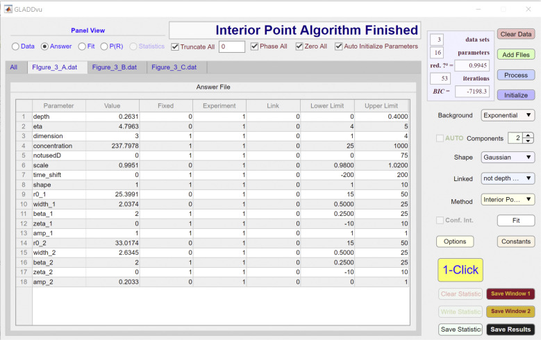
Figure S1.
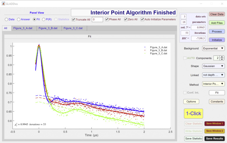
Screenshot of the answer panel for dataset A of GLADDvu during the global analysis of simulated data using model 3. Related to Table 4 and Fig. 4 D.
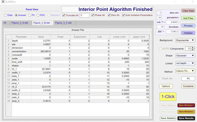
Figure S2.
Screenshot of the answer panel for dataset B of GLADDvu during the global analysis of simulated data using model 3. Related to Table 4 and Fig. 4 D.
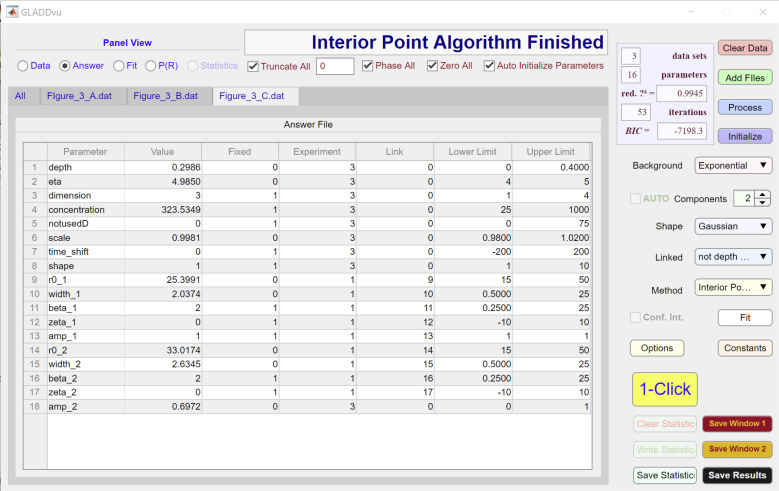
Figure S3.
Screenshot of the answer panel for dataset C of GLADDvu during the global analysis of simulated data using model 3. Related to Table 4 and Fig. 4 D.
The global reduced χ2 value is given by
| (14) |
where is the total number of unique fit parameter values that are varied. As with fitting single datasets, BIC values can be used to select the optimal from a set of models used to fit multiple datasets. Eqs. 9 and 10 for AICc and BIC, respectively, both assume that the variance of the data is constant for all data points. Although this assumption is valid for DEER data from a single experiment that has not been background corrected, data from different experiments that are being globally analyzed will have different noise levels. Cavanaugh and Neath (1999) have shown that the derivation of the BIC does not require the assumption that the noise is identically distributed for all data points. Following Banks and Joyner (2017), we assume that each point in a given DEER dataset, j, has a variance to give
| (15) |
where is the total number of data points in the global analysis and is the total number of unique fit parameter values that are varied.
Table 4 shows the statistics obtained from fitting the three simulated datasets in Fig. 4 using six different models. Models 2, 4, and 6 use n = 1, 2, and 3 Gaussian components, each corresponding to a separate conformation with no parameters linked. Thus, these models are equivalent to fitting the data individually. For models 1, 3, and 5, all of the and values are linked, and the same set of Gaussian components is used to fit both datasets. Although the most complex model, 6, with gives the lowest SSR and values, model 3 with gives the lowest BIC values and is strongly preferred.
Table 4. Model statistics from fitting simulated data in Fig. 4.
| Model | n | Linked | q | SSR | BIC | ΔBIC | |
|---|---|---|---|---|---|---|---|
| 1 | 1 | r0 and σr | 11 | 0.13044 | 1.7759 | -6776.0 | 422.3 |
| 2 | 1 | Nothing | 15 | 0.08557 | 1.1268 | -7106.9 | 91.4 |
| 3 | 2 | r0 and σr | 16 | 0.07588 | 0.9945 | -7198.3 | 0.0 |
| 4 | 2 | Nothing | 24 | 0.07503 | 0.9945 | -7153.3 | 45.1 |
| 5 | 3 | r0 and σr | 21 | 0.07532 | 0.9944 | -7170.2 | 28.1 |
| 6 | 3 | Nothing | 33 | 0.07377 | 0.9878 | -7108.0 | 90.3 |
The models differ in the number of Gaussian components, n, used to define the distance distributions and in how their parameters are linked for the different datasets. In all models, the modulation depths, Δ, and the background parameters, η, for the different datasets are not linked. A video (Video 3) demonstrating the use of GLADDvu to perform the fits of these simulated data is available.
A core principle of global analysis is that the models tested should move beyond mathematical statements about the functions and parameter sets used to fit data and incorporate the fundamental biological questions being addressed in the experiments (Beechem et al., 1991; Beechem, 1992). Moving beyond loose interpretations of the peaks in the P(R) obtained from individual fits, the results in Fig. 4 and Table 4 allow a DEER practitioner to confidently assert that the data are consistent with, and in fact optimally modeled, as a protein undergoing a ligand-dependent shift in the equilibrium between two conformational states that are themselves ligand independent.
With the recent development of the DeerLab software package (Ibáñez et al., 2020), it is now possible to perform a global analysis of DEER data using Tikhonov regularization. The results of such an analysis of these three simulated datasets are shown in Fig. S4. Note that unlike model-based fitting (Fig. 4 E), the regularization-based global analysis (Fig. S4 C) does not correctly disentangle the two component distributions corresponding to the two conformations in equilibrium. In this tutorial, we focus on the use of our GLADDvu software for the model-based global analysis of DEER data.
Figure S4.
Global analysis of the same simulated DEER data as in Fig. 4 using Tikhonov regularization. (A) The data are shown as filled circles. The best-fit lines for model 3 (R0 and σR values linked) are shown as solid black lines. The dashed colored lines were obtained using DeerLab version 0.13.2 (Ibáñez et al., 2020) to perform a global analysis using nonparametric distance distributions based on Tikhonov regularization. (B) P(R) from DeerLab for datasets A (red), B (green), and C (blue). The black lines are the true P(R) used for the simulations. (C) The P'(R) of the underlying components of the global analysis obtained from DeerLab are shown in cyan, and the true P'(R) used for the simulations are superimposed as shaded regions. The global Tikhonov fit with unconstrained fractions of the conformations does not recover the proper distributions of the hypothetical pure conformational states if traces representing the pure conformations are not included in the data. The model-based approach (Fig. 4) does recover the pure conformational states because it favors P'(R) with a minimum number of components. If applicable, a chemical equilibrium model and Tikhonov regularization, as is possible with DeerLab, effectively constrains the mole fractions and can recover the true P'(R).
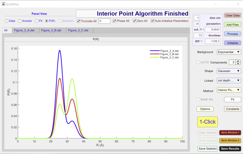
A description of how parameters are linked in GLADDvu is provided in the Appendix. Screenshots showing the use of GLADDvu to fit these simulated datasets to model 3 are shown in Figs. S1, S2, S3, S5, and S6. A demonstration of the use of GLADDvu to perform all of the fits listed in Table 4 is available in Video 3.
Figure S5.
Screenshot of the fit panel of GLADDvu during the global analysis of simulated data using model 3. Related to Table 4 and Fig. 4 D.
Figure S6.
Screenshot of the P(R) panel of GLADDvu during the global analysis of simulated data using model 3. Related to Table 4 and Fig. 4 D.
Video 3.
Demonstration of the use of GLADDvu (https://github.com/erichustedt/GLADDvu) to perform the model-based global analysis of three simulated datasets. The fits to the six different models listed in Table 4 are performed. The optimal results, as determined by BIC values, were obtained for model 3 and are shown in Fig. 4. The datasets (Fig. 4, A–C) are available for dowload.
Global analysis of DEER data
Global analysis has long been used to fit both linear and saturation transfer EPR continuous wave EPR data to determine parameters defining either the global rotational diffusion (Hustedt et al., 1993; Hustedt and Beth, 1995, 2001; Stein et al., 2002; Hustedt and Beth, 2004) or the distance between and relative orientation (Hustedt and Beth, 1996; Hustedt et al., 1997; Hustedt and Beth, 1999; Ghimire et al., 2012; Sahu et al., 2014) of spin labels. In an early example of the use of global analysis for DEER data, Goldfarb and colleagues investigated the cAMP-induced conformational change in the carboxy-terminal cyclic nucleotide binding domain (NBD) of the HCN2 ion channel (Collauto et al., 2017). A total of 26 DEER datasets collected either at equilibrium as a function of cAMP concentration or at varying time points following addition of stoichiometric cAMP using a microfluidic rapid freeze quench apparatus. All datasets were fit with three Gaussian components representing two different conformations: open and closed. The centers and widths of the three Gaussians and the relative amplitude of the two Gaussian components representing the open state were linked. The relative fractions of the open versus closed states were varied across the different datasets. Modeling the ligand-induced conformational transition using a four-state model,
the fractions of the open and closed conformations were used to quantify the three corresponding equilibrium constants and to estimate the six transition rates.
Mchaourab and coworkers have globally analyzed DEER data to investigate the ligand-dependent functional dynamics of a number of membrane transporters, including ion-dependent secondary transporters (Masureel et al., 2014; Dastvan et al., 2016; Martens et al., 2016; Claxton et al., 2018; Paz et al., 2018; Jagessar et al., 2020) and ATP-dependent multidrug transporters (Mishra et al., 2014; Verhalen et al., 2017; Dastvan et al., 2019). Using previously published data, we present below details of how global analysis has advanced the understanding of ligand-dependent conformational equilibrium in a way that would not be possible from the individual fits.
P-glycoprotein 1 (Pgp)
The use of DEER to investigate the conformational dynamics of the ABC transporter Pgp provides an instructive example of the benefits of global analysis. Although the initial DEER study was performed on the basis of a single crystal structure (Verhalen et al., 2017), the recent determination of multiple cryo-EM structures (Alam et al., 2018; Kim and Chen, 2018; Alam et al., 2019) illustrates the unique and complementary insight contributed by DEER analysis (Dastvan et al., 2019). Pgp is a mammalian ATP-binding cassette transporter capable of pumping a wide array of xenobiotic substrates out of cells (Aller et al., 2009; Jin et al., 2012; Li et al., 2014; Kim and Chen, 2018). Moreover, a number of inhibitors have been developed in search of a strategy to increase the efficacy of cancer chemotherapy (Chufan et al., 2016). Here, we focus on data collected in the presence of different substrates and inhibitors of Pgp.
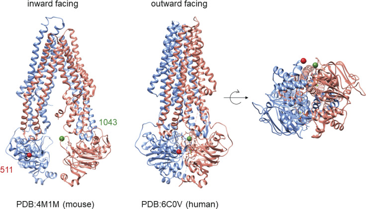
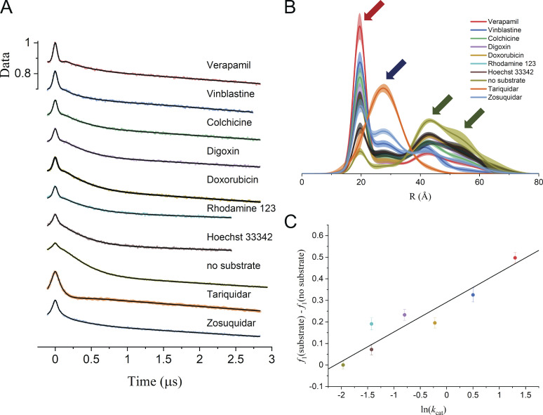
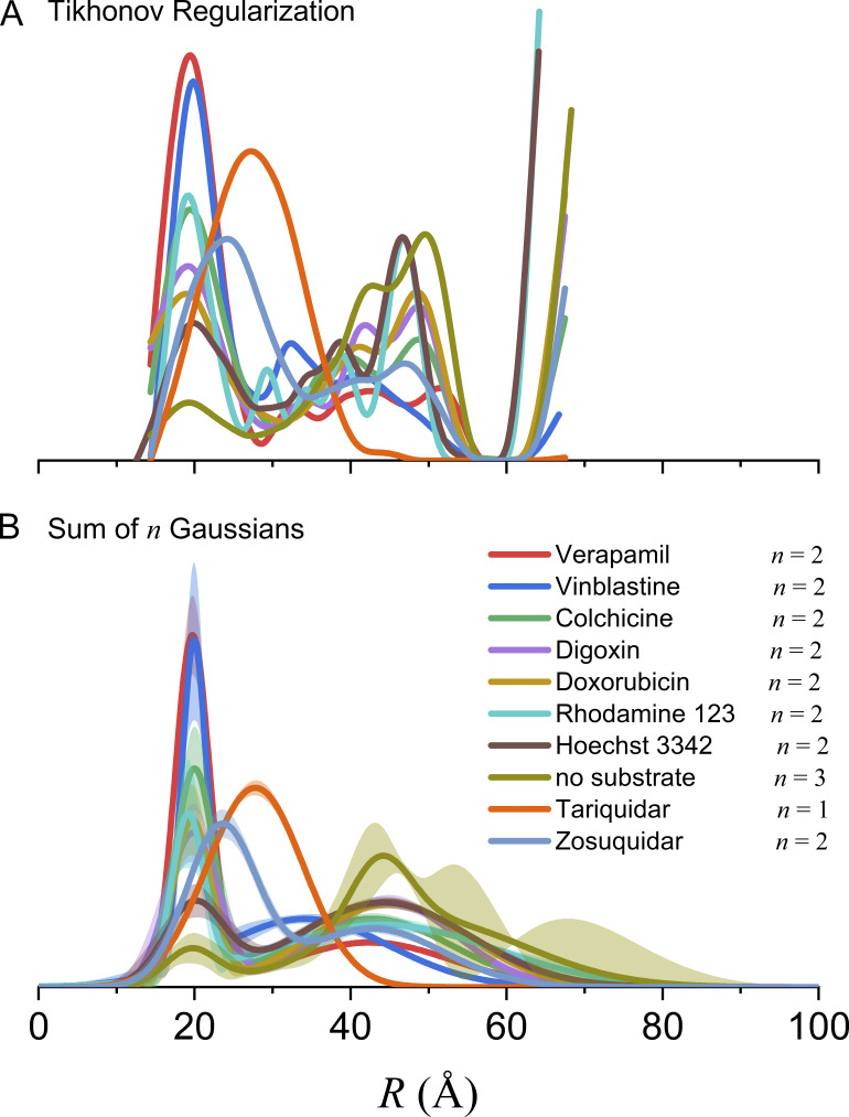
An extensive set of spin label pairs was introduced to study the functional dynamics of Pgp under different biochemical conditions that favor specific conformational states (Verhalen et al., 2017; Dastvan et al., 2019). Here, we focus on a pair of sites, 511 and 1043, within NBDs 1 and 2, respectively, which come together to form two nucleotide binding sites (NBS; Fig. 5). In the presence of ATP and inorganic vanadate (Vi), Pgp can form a state that mimics the post-hydrolysis transition state where ADP and phosphate are trapped in the binding sites. Under these conditions, DEER data from Pgp show an equilibrium between distinctly different conformational states (Verhalen et al., 2017) dependent on the substrate present. Fig. 6 shows 10 DEER traces collected for Pgp labeled at 511/1043 in the presence of ATP/Vi and either no substrate, 7 different substrates, or 2 inhibitors of transport (Dastvan et al., 2019).
Figure 5.
The conformational shift of Pgp. Left: The mouse Pgp structure in the inward-facing conformation (Li et al., 2014). Highlighted are two residues, 511 and 1043, which are on opposite halves of Pgp. Middle: The structure of human Pgp in the outward-facing conformation (Kim and Chen, 2018). Right: The closure of the NBDs is shown in detail, highlighting the nearness of the residues 511 and 1043 in the outward-facing conformation. PDB, Protein Data Bank.
Figure 6.
Global analysis of Q-band DEER data for Pgp spin labeled with MTSSL at residues 511 and 1043. (A) Samples were prepared in mixed micelles with ATP and Vi in the presence and absence of substrates and inhibitors as indicated (Dastvan et al., 2019). The scaled data are shown as filled colored circles, and the best fits obtained from global analysis using model 2 (Table 5) are shown as solid black lines. (B) The best-distance distributions obtained using model 2 to fit the Pgp data with the associated 2σ (95%) confidence bands as shaded regions. The R0 values of the four components are indicated by the arrows. (C) The substrate-induced population of the shortest distance component is correlated with the activation energy of ATP turnover.
The analysis of these 10 datasets individually using either Tikhonov regularization or model-based fitting gives broad multicomponent distance distributions that depend strongly on the substrate (Fig. S7). Using either approach, however, it is difficult to draw firm conclusions about the conformations evident in these distributions. To test the utility of global analysis for these data, three different models were used in combined fits (Table 5). Models 1 and 2 employ three and four conformational states, respectively, each modeled as a single Gaussian component. The and values of these Gaussians were linked across all 10 datasets while the amplitudes of the components, the modulation depths, background factors, and scale factors varied. For the conformation with the shortest mean interspin distance, the two NBDs are tightly bound together, trapping ADP/Vi within NBS 2. The intermediate distance component (and its corresponding conformation) is highly populated only in the presence of the two inhibitors, tariquidar and zosuquidar, or vinblastine, which can act as an inhibitor at high concentrations. The two components with the longest mean distances correspond to those seen in the absence of any nucleotide (apo state). Model 3 specifically tests whether the apo-like contributions to P(R), evident at the longer distances, can be fit as a single conformation modeled by two Gaussian components with a linked ratio across all conditions. Based on the values in Table 5, model 2 is the optimal model. The increase in BIC for model 3 versus model 2 indicates that there are distinct apo-like conformations for different substrates. The separation of these underlying conformational states is much clearer using model-based global analysis, and the quality of the fits in Fig. 6 A suggests that, indeed, there is a common set of protein conformations across all 10 experimental conditions.
Figure S7.
Distance distributions from individual fits to the DEER data for Pgp in Fig. 6. (A) The model-free P(R) were obtained using Tikhonov regularization in DeerAnalysis 2019 (Jeschke et al., 2006). The optimal regularization factor was determined by generalized cross-validation and the starting time point for background fitting using the validation tool. (B) The model-based P(R) were obtained assuming a 3-D exponential background and using Gaussian components in DD (Brandon et al., 2012; Stein et al., 2015; Hustedt et al., 2018). The optimal number of Gaussians, n, was determined using BIC values.
Table 5. Statistics of fitting Pgp data (Fig. 6).
| Model | n | Linked | q | SSR | BICWLS | ΔBICWLS | |
|---|---|---|---|---|---|---|---|
| 1 | 3 | Gaussians | 56 | 2.5980E-02 | 1.2183 | −36,842.8 | 62.2 |
| 2 | 4 | Gaussians | 68 | 2.4681E-02 | 1.1593 | −36,905.0 | 0.0 |
| 3 | 4 | Gaussians and ratio of two longest | 59 | 2.5623E-02 | 1.1921 | −36,885.7 | 19.3 |
The models differ in the number of Gaussian components, n, used to define the distance distributions and in how their parameters are linked for the different datasets. In all models, the modulation depths, Δ, and the background parameters, η, for the different datasets are not linked. A video (Video 4) demonstrating the use of GLADDvu to perform the fits of these Pgp data is available.
Global analysis also allows enhanced quantitative analysis of the relative populations of the various conformations. Those substrates that induced the largest population of the tightly bound component were most efficient in stimulating ATP turnover, resulting in a linear relationship between this component’s population and the natural logarithm of stimulated ATP turnover rate constant, kcat (Fig. 6 C; Dastvan et al., 2019). These results demonstrate that, using global analysis, the equilibrium populations of protein conformations determined from the global analysis of DEER data can be quantitatively related to the function dynamics of the protein and that important mechanistic insights can be obtained.
A demonstration of the use of GLADDvu to perform the fits of these Pgp datasets to models 1–3 is available in Video 4.
Video 4.
Demonstration of the use of GLADDvu (https://github.com/erichustedt/GLADDvu) to perform the model-based global analysis of the Pgp datasets. The fits to the three different models listed in Table 5 are perforrmed. The optimal results, as determined by BIC values, were obtained for model 2 and are shown in Fig. 6.
LmrP
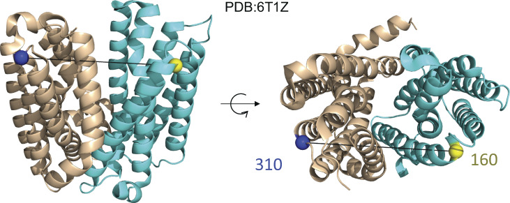
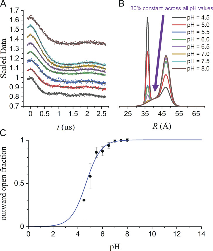
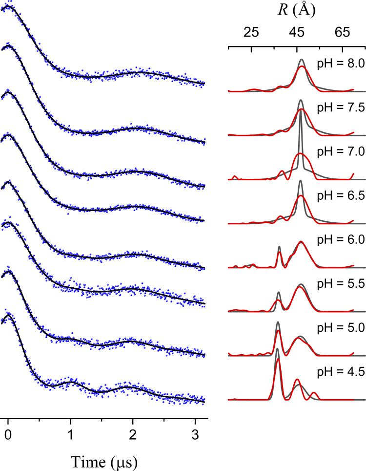
LmrP is a multidrug transporter from Lactococcus lactis and a member of the major facilitator superfamily whose transport is driven by the proton gradient (Fig. 7; van Veen et al., 1999; van Veen, 2001). In a series of papers, DEER spectroscopy has been used to define the protonation-dependent isomerization of the transporter between inward-facing and outward-facing conformations (Masureel et al., 2014; Martens et al., 2016; Debruycker et al., 2020). Fig. 8 shows DEER data from LmrP collected at eight different pH values with labels placed at residues L160C and I310C at the extracellular ends of TM helices 5 and 10, respectively. In Fig. S8, the individual DEER traces have been analyzed using both model-based and model-free approaches. Collectively, these data are qualitatively consistent with a model where TM helices 5 and 10 move closer and become more ordered, closing the extracellular gate, as residues within the pore are protonated. The shift from the OO to OC state is reflected in a transition from a broad unimodal at pH 8.0 centered at ∼46 Å to a multimodal P(R) at pH 4.6 with a narrower component centered at ∼37 Å. This qualitative interpretation of these data raises the question of whether they are consistent with a single set of conformations of the protein, OO and OC, which would give rise to an ideal pair of distributions, and respectively. If so, for each of the corresponding to the eight datasets
where is the pH-dependent fraction of the protein in the OO conformation. and can be used for modeling the two conformational states of the protein, and the set of can be used for quantifying the equilibrium between the two conformations, providing a measure of the pH dependence of the stability of the two conformations.
Figure 7.
X-ray crystal structure of LmrP. Related to Debruycker et al. (2020). On the left is a side view of LmrP, and on the right is the top (extracellular) view of LmrP. Highlighted are two residues, 160 and 310, on opposite halves of LmrP where spin labels have been placed. PDB, Protein Data Bank.
Figure 8.
Global analysis of Q-band DEER data for LmrP spin labeled with MTSSL at residues 160 and 310. Related to Masureel et al. (2014). Samples were prepared in dodecyl maltoside micelles at eight different pH values ranging from 4.5 to 8.0 as indicated. (A) Overlay of all eight datasets and the fits obtained from global analysis using model 7 in Table 6. (B) The P(R) obtained for model 7. (C) The OO fraction obtained for model 7 as a function of pH fit to determine the pK value.
Figure S8.
Results from individual fits for LmrP data in Fig. 8. On the left, the data are shown as black dots with the individual model-based fits as blue lines. The corresponding P(R) are shown (black lines) on the right together with those obtained from Tikhonov regularization using DeerAnalysis 2019 (Jeschke et al., 2006; red lines). The widths of the narrow components at pH 6.5 and 7.0 have large relative uncertainties, and owing to the fact that the modulation is not fully damped over the measured evolution time.
Using the model-based approach, all of the DEER traces with the exception of the pH 6.0 data are optimally fit with n = 2 Gaussian components. At the lower pH values, the two components with means separated by ∼10 Å clearly correspond to OC and OO conformations. At the higher pH values, the two components have similar values, one broad and one narrow. These results suggest that three Gaussian components will be needed for the optimal global fit to the eight traces and raise the question of what the broad component evident at higher pH values represents.
The full set of models tested against the eight LmrP DEER traces are listed in Table 6. Models 1 and 2 fit the datasets individually with two or three Gaussian components and no parameters linked. Models 3 and 4 fit the data globally with two or three conformations, with each modeled as a single Gaussian component. For these models, the values of and are linked across all datasets, and the amplitudes, modulation depths, backgrounds, and scale factors are not linked. Models 5, 6, and 7 all use three Gaussians with the values of and linked and different ways of linking some of the amplitude variables. For model 5, the OC conformation is modeled by a single Gaussian, and the OO conformation is modeled by two Gaussians, with a linked ratio across all eight traces. For model 6, the OO conformation is modeled by a single Gaussian, and the OC conformation is modeled by two Gaussians, with a linked ratio across all eight traces. For model 7, the OO and OC conformations are both modeled by single Gaussians, and a third component contributes a linked fraction across all eight datasets.
Table 6. Models used to fit LmrP data (Fig. 8).
| Model | n | Linked | q | SSR | BICWLS | ΔBICWLS | pK | |
|---|---|---|---|---|---|---|---|---|
| 1 | 2 | Nothing | 64 | 0.075598 | 1.1230 | −30,382.8 | 139.7 | — |
| 2 | 3 | Nothing | 88 | 0.074582 | 1.1129 | −30,242.2 | 280.4 | — |
| 3 | 2 | Gaussians | 36 | 0.079455 | 1.1651 | −30,474.8 | 47.7 | 4.6 ± 0.6 |
| 4 | 3 | Gaussians | 46 | 0.077139 | 1.1329 | −30,483.0 | 39.6 | — |
| 5 | 3 | Custom | 39 | 0.078279 | 1.1463 | −30,498.7 | 23.8 | 4.6 ± 0.7 |
| 6 | 3 | Custom | 39 | 0.078139 | 1.1419 | −30,509.5 | 13.1 | 4.8 ± 1.0 |
| 7 | 3 | Custom | 39 | 0.077450 | 1.1365 | −30,522.6 | 0.0 | 4.7 ± 1.3 |
The models differ in the number of Gaussian components, n, used to define the distance distributions and in how their parameters are linked for the different datasets. In all models, the modulation depths, Δ, and the background parameters, η, for the different datasets are not linked. pK values are the negative logarithms of the dissociation constants.
Of the seven models tested, model 7 is optimal according to the BIC values (Table 6). Model 7 fits the data to n = 3 Gaussian components (Fig. 8). For two of these, the fractional contribution is pH dependent, one corresponding to OC state and one corresponding to the OO state The fractional contribution of the third Gaussian is independent of pH. This third component could account for one or more of a number of factors, including non-Gaussian character of the true deviation of the background factors from true exponentials, or the presence of nonfunctional protein in the sample. Assuming the latter, the fraction of OO functional protein have been plotted and fit to determine a pK for the transition between the two conformations. Significantly, when the appropriate values of are fit to a titration curve, models 3, 5, 6, and 7 all give similar pK values (Table 6). Although including a third, pH-independent population did not affect the pK determined from the titration, the ability to identify such nonfunctional proteins can in future studies spur changes and optimization of purification protocols.
Looking ahead
GLADDvu was designed to be a fully flexible tool suitable for a wide variety of experimental situations beyond the examples presented in this tutorial. These examples demonstrated how global analysis of DEER data from one spin-labeled mutant obtained under different ligand conditions gives enhanced qualitative insights into the functionally relevant dynamics of integral membrane proteins complete with error analysis of the fit parameters. One could consider analyzing data from multiple mutants under a common set of ligand conditions with different and a common set of Such analyses would test whether domains are moving as rigid bodies or whether the spin labels have any influence on equilibrium coefficients.
The model-based approach available with GLADDvu allows the ligand-dependent fractions of various components to be determined by the fit while providing the uncertainties of the parameters as well as the confidence bands for the distance distributions. Recently, a model-free approach to the global analysis of DEER data has been developed (Ibáñez and Jeschke, 2020; Ibáñez et al., 2020). As is the case for the analysis of individual time traces, different approaches to the global analysis of multiple datasets will provide complementary insights into the fundamental biological issues under investigation.
Online supplemental material
Fig. S1 shows a screenshot of the answer panel for dataset A of GLADDvu during the global analysis of simulated data using model 3. Fig. S2 shows a screenshot of the answer panel for dataset B of GLADDvu during the global analysis of simulated data using model 3. Fig. S3 shows a screenshot of the answer panel for dataset C of GLADDvu during the global analysis of simulated data using model 3. Fig. S4 shows a global analysis of the same simulated DEER data as in Fig. 4 using Tikhonov regularization. Fig. S5 shows a screenshot of the Fit panel of GLADDvu during the global analysis of simulated data using model 3. Fig. S6 shows a screenshot of the P(R) panel of GLADDvu during the global analysis of simulated data using model 3. Fig. S7 shows distance distributions from individual fits to the DEER data for Pgp in Fig. 6. Fig. S8 shows results from individual fits for LmrP data in Fig. 8. Videos 1, 2, 3, and 4 demonstrate the fitting of the data in Fig. 2 using DD and the fitting of the data in Figs. 2, 4, and 6 using GLADDvu, respectively.
Appendix
GLADDvu
Our MATLAB software, DD, for the model-based fitting of single DEER datasets has been described in detail elsewhere (Brandon et al., 2012; Stein et al., 2015; Hustedt et al., 2018). A separate MATLAB program, GLADDvu, has been developed for globally fitting multiple DEER datasets. GLADDvu is designed for maximal flexibility, allowing the user to create both simple and complex models with parameters that are fixed, floated, or linked as desired. A fixed parameter is kept at its initial value and is not varied during the fit. A floated parameter is varied to find the best-fit values that minimize the global reduced χ2 value. A linked parameter for one experimental dataset is required to have the same value as another floated parameter for the same or a different dataset.
After reading in multiple files, each dataset is phased. Then, for each separate experiment, the 0 of the time axis is adjusted such that the signal maximum occurs at and the values of the DEER signal are scaled such that The noise variance for a given dataset, is estimated from the variance of its imaginary component. Various background models can be selected, including exponential, stretched exponential, and excluded volume. The distance distribution can be modeled as the sum of n components (Eq. 6), including Gaussians (Eq. 7). Minimization of is attempted using MATLAB’s interior point, global search, or particle swarm algorithms.
The model used to analyze data are specified by the Background, Components, Shape, and Linked dropdown menus and can be further modified using the individual Answer File spreadsheets for each dataset (Figs. S1, S2, and S3). As seen in the third column of these spreadsheets, for each of the three datasets, there are eight parameters that are floated (i.e., they are not fixed). These are (depth), (eta), (amp_2), and a scale factor (∼1). The and parameters for experiments 2 and 3 are linked to the corresponding parameters for experiment 1, as specified in the fourth and fifth columns of the Answer File spreadsheet, ensuring that the same two Gaussian components are used to define the best-fit P(R) for the two datasets.
The parameter dimension corresponds to d in Eq. 5. For d = 3, concentration is the effective spin concentration assuming a homogeneous 3-D solution of spins for the given modulation depth.
The parameters β and ζ can be used for defining three non-Gaussian component shapes, a generalized normal distribution with nonzero excess kurtosis, a skew normal distribution with nonzero skew, and a generalized skew normal distribution with nonzero excess kurtosis and skew as defined in equations S1–S3 of Hustedt et al. (2018). Here, the parameters are automatically fixed to values, β = 2 and ζ = 0, appropriate for Gaussian components.
The fits to the data and corresponding P(R) are displayed in the fit (Fig. S5) and P(R) (Fig. S6) panels, respectively. Statistics for all fits are displayed in the statistics panel. Videos are provided to demonstrate the use of DD and GLADDvu to perform the fits included in this tutorial.
Acknowledgments
Joseph A. Mindell served as editor.
This work was supported by National Institutes of Health grants GM128087 and GM077659 (H.S. Mchaourab). R.A. Stein was also supported by National Institutes of Health grants GM113195 (M. Maduke), MH070039 (J.E. Gouaux), NS117873 (J. Cordero Morales), GM124310 (A. Rajca), and DC007664 (D. Minor).
The authors declare no competing financial interests.
Author contributions: All authors contributed to the conceptual development of this work. E.J. Hustedt and H.S. Mchaourab wrote the manuscript with the assistance of R.A. Stein. E.J. Hustedt wrote DD and GLADDvu with signficant input from R.A. Stein. R.A. Stein provided all of the experimental data in collaboration with authors of the referenced papers.
References
- Ackermann, K., Wort J.L., and Bode B.E.. 2021. Nanomolar pulse dipolar EPR spectroscopy in proteins: CuII-CuII and nitroxide-nitroxide cases. J. Phys. Chem. B. 125:5358–5364. 10.1021/acs.jpcb.1c03666 [DOI] [PMC free article] [PubMed] [Google Scholar]
- Alam, A., Küng R., Kowal J., McLeod R.A., Tremp N., Broude E.V., Roninson I.B., Stahlberg H., and Locher K.P.. 2018. Structure of a zosuquidar and UIC2-bound human-mouse chimeric ABCB1. Proc. Natl. Acad. Sci. USA. 115:E1973–E1982. 10.1073/pnas.1717044115 [DOI] [PMC free article] [PubMed] [Google Scholar]
- Alam, A., Kowal J., Broude E., Roninson I., and Locher K.P.. 2019. Structural insight into substrate and inhibitor discrimination by human P-glycoprotein. Science. 363:753–756. 10.1126/science.aav7102 [DOI] [PMC free article] [PubMed] [Google Scholar]
- Alexander, N., Bortolus M., Al-Mestarihi A., Mchaourab H., and Meiler J.. 2008. De novo high-resolution protein structure determination from sparse spin-labeling EPR data. Structure. 16:181–195. 10.1016/j.str.2007.11.015 [DOI] [PMC free article] [PubMed] [Google Scholar]
- Alexander, N.S., Stein R.A., Koteiche H.A., Kaufmann K.W., Mchaourab H.S., and Meiler J.. 2013. RosettaEPR: rotamer library for spin label structure and dynamics. PLoS One. 8:e72851. 10.1371/journal.pone.0072851 [DOI] [PMC free article] [PubMed] [Google Scholar]
- Aller, S.G., Yu J., Ward A., Weng Y., Chittaboina S., Zhuo R., Harrell P.M., Trinh Y.T., Zhang Q., Urbatsch I.L., et al. 2009. Structure of P-glycoprotein reveals a molecular basis for poly-specific drug binding. Science. 323:1718–1722. 10.1126/science.1168750 [DOI] [PMC free article] [PubMed] [Google Scholar]
- Amey, J.L., Keeley J., Choudhury T., and Kuprov I.. 2021. Neural network interpretation using descrambler groups. Proc. Natl. Acad. Sci. USA. 118:e2016917118. 10.1073/pnas.2016917118 [DOI] [PMC free article] [PubMed] [Google Scholar]
- Arrigoni, C., Rohaim A., Shaya D., Findeisen F., Stein R.A., Nurva S.R., Mishra S., Mchaourab H.S., and Minor D.L. Jr. 2016. Unfolding of a temperature-sensitive domain controls voltage-gated channel activation. Cell. 164:922–936. 10.1016/j.cell.2016.02.001 [DOI] [PMC free article] [PubMed] [Google Scholar]
- Banks, H.T., and Joyner M.L.. 2017. AIC under the framework of least squares estimation. Appl. Math. Lett. 74:33–45. 10.1016/j.aml.2017.05.005 [DOI] [Google Scholar]
- Barrett, P.J., Song Y., Van Horn W.D., Hustedt E.J., Schafer J.M., Hadziselimovic A., Beel A.J., and Sanders C.R.. 2012. The amyloid precursor protein has a flexible transmembrane domain and binds cholesterol. Science. 336:1168–1171. 10.1126/science.1219988 [DOI] [PMC free article] [PubMed] [Google Scholar]
- Beechem, J.M. 1992. Global analysis of biochemical and biophysical data. Methods Enzymol. 210:37–54. 10.1016/0076-6879(92)10004-W [DOI] [PubMed] [Google Scholar]
- Beechem, J.M., Gratton J.M., Ameloot M., Knutson J.R., and Brand L.. 1991. The global analysis of fluorescence intensity and anisotropy decay data: second generation theory and programs. In Topics in Fluorescence Spectroscopy. Lakowicz J.R., editor. Plenum Press, New York. [Google Scholar]
- Borbat, P.P., and Freed J.H.. 2014. Pulse dipolar electron spin resonance: distance measurements. In Structural Information from Spin-Labels and Intrinsic Paramagnetic Centres in the Biosciences. Timmel C.R., and Harmer J.R., editors. Springer, Berlin. 1–82. [Google Scholar]
- Bowman, M.K., Maryasov A.G., Kim N., and DeRose V.J.. 2004. Visualization of distance distribution from pulsed double electron-electron resonance data. Appl. Magn. Reson. 26:23. 10.1007/BF03166560 [DOI] [Google Scholar]
- Brandon, S., Beth A.H., and Hustedt E.J.. 2012. The global analysis of DEER data. J. Magn. Reson. 218:93–104. 10.1016/j.jmr.2012.03.006 [DOI] [PMC free article] [PubMed] [Google Scholar]
- Burnham, K.P., and Anderson D.R.. 2002. Model Selection and Multimodel Inference: A Practical Information-Theoretic Approach. Second edition. Springer-Verlag, New York. [Google Scholar]
- Cavanaugh, J.E., and Neath A.A.. 1999. Generalizing the derivation of the Schwarz information criterion. Commun. Stat. Theory Methods. 28:49–66. 10.1080/03610929908832282 [DOI] [Google Scholar]
- Chiang, Y.W., Borbat P.P., and Freed J.H.. 2005. The determination of pair distance distributions by pulsed ESR using Tikhonov regularization. J. Magn. Reson. 172:279–295. 10.1016/j.jmr.2004.10.012 [DOI] [PubMed] [Google Scholar]
- Chufan, E.E., Kapoor K., and Ambudkar S.V.. 2016. Drug-protein hydrogen bonds govern the inhibition of the ATP hydrolysis of the multidrug transporter P-glycoprotein. Biochem. Pharmacol. 101:40–53. 10.1016/j.bcp.2015.12.007 [DOI] [PMC free article] [PubMed] [Google Scholar]
- Claxton, D.P., Quick M., Shi L., de Carvalho F.D., Weinstein H., Javitch J.A., and Mchaourab H.S.. 2010. Ion/substrate-dependent conformational dynamics of a bacterial homolog of neurotransmitter:sodium symporters. Nat. Struct. Mol. Biol. 17:822–829. 10.1038/nsmb.1854 [DOI] [PMC free article] [PubMed] [Google Scholar]
- Claxton, D.P., Kazmier K., Mishra S., and Mchaourab H.S.. 2015. Navigating membrane protein structure, dynamics, and energy landscapes using spin labeling and EPR spectroscopy. Methods Enzymol. 564:349–387. 10.1016/bs.mie.2015.07.026 [DOI] [PMC free article] [PubMed] [Google Scholar]
- Claxton, D.P., Jagessar K.L., Steed P.R., Stein R.A., and Mchaourab H.S.. 2018. Sodium and proton coupling in the conformational cycle of a MATE antiporter from Vibrio cholerae. Proc. Natl. Acad. Sci. USA. 115:E6182–E6190. 10.1073/pnas.1802417115 [DOI] [PMC free article] [PubMed] [Google Scholar]
- Collauto, A., DeBerg H.A., Kaufmann R., Zagotta W.N., Stoll S., and Goldfarb D.. 2017. Rates and equilibrium constants of the ligand-induced conformational transition of an HCN ion channel protein domain determined by DEER spectroscopy. Phys. Chem. Chem. Phys. 19:15324–15334. 10.1039/C7CP01925D [DOI] [PMC free article] [PubMed] [Google Scholar]
- Dalmas, O., Sandtner W., Medovoy D., Frezza L., Bezanilla F., and Perozo E.. 2014. A repulsion mechanism explains magnesium permeation and selectivity in CorA. Proc. Natl. Acad. Sci. USA. 111:3002–3007. 10.1073/pnas.1319054111 [DOI] [PMC free article] [PubMed] [Google Scholar]
- Dastvan, R., Fischer A.W., Mishra S., Meiler J., and Mchaourab H.S.. 2016. Protonation-dependent conformational dynamics of the multidrug transporter EmrE. Proc. Natl. Acad. Sci. USA. 113:1220–1225. 10.1073/pnas.1520431113 [DOI] [PMC free article] [PubMed] [Google Scholar]
- Dastvan, R., Mishra S., Peskova Y.B., Nakamoto R.K., and Mchaourab H.S.. 2019. Mechanism of allosteric modulation of P-glycoprotein by transport substrates and inhibitors. Science. 364:689–692. 10.1126/science.aav9406 [DOI] [PMC free article] [PubMed] [Google Scholar]
- Debruycker, V., Hutchin A., Masureel M., Ficici E., Martens C., Legrand P., Stein R.A., Mchaourab H.S., Faraldo-Gómez J.D., Remaut H., et al. 2020. An embedded lipid in the multidrug transporter LmrP suggests a mechanism for polyspecificity. Nat. Struct. Mol. Biol. 27:829–835. 10.1038/s41594-020-0464-y [DOI] [PMC free article] [PubMed] [Google Scholar]
- Dellisanti, C.D., Ghosh B., Hanson S.M., Raspanti J.M., Grant V.A., Diarra G.M., Schuh A.M., Satyshur K., Klug C.S., and Czajkowski C.. 2013. Site-directed spin labeling reveals pentameric ligand-gated ion channel gating motions. PLoS Biol. 11:e1001714. 10.1371/journal.pbio.1001714 [DOI] [PMC free article] [PubMed] [Google Scholar]
- Dürr, K.L., Chen L., Stein R.A., De Zorzi R., Folea I.M., Walz T., Mchaourab H.S., and Gouaux E.. 2014. Structure and dynamics of AMPA receptor GluA2 in resting, pre-open, and desensitized states. Cell. 158:778–792. 10.1016/j.cell.2014.07.023 [DOI] [PMC free article] [PubMed] [Google Scholar]
- Edwards, T.H., and Stoll S.. 2016. A Bayesian approach to quantifying uncertainty from experimental noise in DEER spectroscopy. J. Magn. Reson. 270:87–97. 10.1016/j.jmr.2016.06.021 [DOI] [PMC free article] [PubMed] [Google Scholar]
- Edwards, T.H., and Stoll S.. 2018. Optimal Tikhonov regularization for DEER spectroscopy. J. Magn. Reson. 288:58–68. 10.1016/j.jmr.2018.01.021 [DOI] [PMC free article] [PubMed] [Google Scholar]
- Edwards, S.J., Moth C.W., Kim S., Brandon S., Zhou Z., Cobb C.E., Hustedt E.J., Beth A.H., Smith J.A., and Lybrand T.P.. 2014. Automated structure refinement for a protein heterodimer complex using limited EPR spectroscopic data and a rigid-body docking algorithm: a three-dimensional model for an ankyrin-CDB3 complex. J. Phys. Chem. B. 118:4717–4726. 10.1021/jp4099705 [DOI] [PMC free article] [PubMed] [Google Scholar]
- Elgeti, M., and Hubbell W.L.. 2021. DEER analysis of GPCR conformational heterogeneity. Biomolecules. 11:778. 10.3390/biom11060778 [DOI] [PMC free article] [PubMed] [Google Scholar]
- Evans, E.G.B., Morgan J.L.W., DiMaio F., Zagotta W.N., and Stoll S.. 2020. Allosteric conformational change of a cyclic nucleotide-gated ion channel revealed by DEER spectroscopy. Proc. Natl. Acad. Sci. USA. 117:10839–10847. 10.1073/pnas.1916375117 [DOI] [PMC free article] [PubMed] [Google Scholar]
- Gamble Jarvi, A., Bogetti X., Singewald K., Ghosh S., and Saxena S.. 2021. Going the dHis-tance: site-directed Cu2+ labeling of proteins and nucleic acids. Acc. Chem. Res. 54:1481–1491. 10.1021/acs.accounts.0c00761 [DOI] [PubMed] [Google Scholar]
- Georgieva, E.R., Borbat P.P., Ginter C., Freed J.H., and Boudker O.. 2013. Conformational ensemble of the sodium-coupled aspartate transporter. Nat. Struct. Mol. Biol. 20:215–221. 10.1038/nsmb.2494 [DOI] [PMC free article] [PubMed] [Google Scholar]
- Ghimire, H., Hustedt E.J., Sahu I.D., Inbaraj J.J., McCarrick R., Mayo D.J., Benedikt M.R., Lee R.T., Grosser S.M., and Lorigan G.A.. 2012. Distance measurements on a dual-labeled TOAC AChR M2δ peptide in mechanically aligned DMPC bilayers via dipolar broadening CW-EPR spectroscopy. J. Phys. Chem. B. 116:3866–3873. 10.1021/jp212272d [DOI] [PMC free article] [PubMed] [Google Scholar]
- Göddeke, H., Timachi M.H., Hutter C.A.J., Galazzo L., Seeger M.A., Karttunen M., Bordignon E., and Schäfer L.V.. 2018. Atomistic mechanism of large-scale conformational transition in a heterodimeric ABC exporter. J. Am. Chem. Soc. 140:4543–4551. 10.1021/jacs.7b12944 [DOI] [PubMed] [Google Scholar]
- Hilger, D., Jung H., Padan E., Wegener C., Vogel K.P., Steinhoff H.J., and Jeschke G.. 2005. Assessing oligomerization of membrane proteins by four-pulse DEER: pH-dependent dimerization of NhaA Na+/H+ antiporter of E. coli. Biophys. J. 89:1328–1338. 10.1529/biophysj.105.062232 [DOI] [PMC free article] [PubMed] [Google Scholar]
- Hilger, D., Polyhach Y., Padan E., Jung H., and Jeschke G.. 2007. High-resolution structure of a Na+/H+ antiporter dimer obtained by pulsed electron paramagnetic resonance distance measurements. Biophys. J. 93:3675–3683. 10.1529/biophysj.107.109769 [DOI] [PMC free article] [PubMed] [Google Scholar]
- Hustedt, E.J., and Beth A.H.. 1995. Analysis of saturation transfer electron paramagnetic resonance spectra of a spin-labeled integral membrane protein, band 3, in terms of the uniaxial rotational diffusion model. Biophys. J. 69:1409–1423. 10.1016/S0006-3495(95)80010-X [DOI] [PMC free article] [PubMed] [Google Scholar]
- Hustedt, E.J., and Beth A.H.. 1996. Determination of the orientation of a band 3 affinity spin-label relative to the membrane normal axis of the human erythrocyte. Biochemistry. 35:6944–6954. 10.1021/bi9601518 [DOI] [PubMed] [Google Scholar]
- Hustedt, E.J., and Beth A.H.. 1999. Nitroxide spin-spin interactions: applications to protein structure and dynamics. Annu. Rev. Biophys. Biomol. Struct. 28:129–153. 10.1146/annurev.biophys.28.1.129 [DOI] [PubMed] [Google Scholar]
- Hustedt, E.J., and Beth A.H.. 2001. The sensitivity of saturation transfer electron paramagnetic resonance spectra to restricted amplitude uniaxial rotational diffusion. Biophys. J. 81:3156–3165. 10.1016/S0006-3495(01)75952-8 [DOI] [PMC free article] [PubMed] [Google Scholar]
- Hustedt, E.J., and Beth A.H.. 2004. High field/high frequency saturation transfer electron paramagnetic resonance spectroscopy: increased sensitivity to very slow rotational motions. Biophys. J. 86:3940–3950. 10.1529/biophysj.103.035048 [DOI] [PMC free article] [PubMed] [Google Scholar]
- Hustedt, E.J., Cobb C.E., Beth A.H., and Beechem J.M.. 1993. Measurement of rotational dynamics by the simultaneous nonlinear analysis of optical and EPR data. Biophys. J. 64:614–621. 10.1016/S0006-3495(93)81420-6 [DOI] [PMC free article] [PubMed] [Google Scholar]
- Hustedt, E.J., Smirnov A.I., Laub C.F., Cobb C.E., and Beth A.H.. 1997. Molecular distances from dipolar coupled spin-labels: the global analysis of multifrequency continuous wave electron paramagnetic resonance data. Biophys. J. 72:1861–1877. 10.1016/S0006-3495(97)78832-5 [DOI] [PMC free article] [PubMed] [Google Scholar]
- Hustedt, E.J., Marinelli F., Stein R.A., Faraldo-Gómez J.D., and Mchaourab H.S.. 2018. Confidence analysis of DEER data and its structural interpretation with ensemble-biased metadynamics. Biophys. J. 115:1200–1216. 10.1016/j.bpj.2018.08.008 [DOI] [PMC free article] [PubMed] [Google Scholar]
- Ibáñez, L.F., and Jeschke G.. 2019. General regularization framework for DEER spectroscopy. J. Magn. Reson. 300:28–40. 10.1016/j.jmr.2019.01.008 [DOI] [PubMed] [Google Scholar]
- Ibáñez, L.F., and Jeschke G.. 2020. Optimal background treatment in pulse dipolar spectroscopy. Phys. Chem. Chem. Phys. 22:1855–1868. [DOI] [PubMed] [Google Scholar]
- Ibáñez, L.F., Jeschke G., and Stoll S.. 2020. DeerLab: a comprehensive software package for analyzing dipolar electron paramagnetic resonance spectroscopy data. Magn. Reson. (Gott.). 1:209–224. 10.5194/mr-1-209-2020 [DOI] [PMC free article] [PubMed] [Google Scholar]
- Jagessar, K.L., Claxton D.P., Stein R.A., and Mchaourab H.S.. 2020. Sequence and structural determinants of ligand-dependent alternating access of a MATE transporter. Proc. Natl. Acad. Sci. USA. 117:4732–4740. 10.1073/pnas.1917139117 [DOI] [PMC free article] [PubMed] [Google Scholar]
- Jeschke, G. 2012. DEER distance measurements on proteins. Annu. Rev. Phys. Chem. 63:419–446. [DOI] [PubMed] [Google Scholar]
- Jeschke, G. 2014. Interpretation of dipolar EPR data in terms of protein structure. In Structural Information from Spin-Labels and Intrinsic Paramagnetic Centres in the Biosciences. Timmel C.R., and Harmer J.R., editors. Springer, Berlin. 83–120. [Google Scholar]
- Jeschke, G. 2016. Ensemble models of proteins and protein domains based on distance distribution restraints. Proteins. 84:544–560. 10.1002/prot.25000 [DOI] [PubMed] [Google Scholar]
- Jeschke, G. 2018a. The contribution of modern EPR to structural biology. Emerg. Top. Life Sci. 2:9–18. 10.1042/ETLS20170143 [DOI] [PMC free article] [PubMed] [Google Scholar]
- Jeschke, G. 2018b. MMM: A toolbox for integrative structure modeling. Protein Sci. 27:76–85. 10.1002/pro.3269 [DOI] [PMC free article] [PubMed] [Google Scholar]
- Jeschke, G., Chechik V., Ionita P., Godt A., Zimmermann H., Banham J., Timmel C.R., Hilger D., and Jung H.. 2006. DeerAnalysis2006—a comprehensive software package for analyzing pulsed ELDOR data. Appl. Magn. Reson. 30:473–498. 10.1007/BF03166213 [DOI] [Google Scholar]
- Jin, M.S., Oldham M.L., Zhang Q., and Chen J.. 2012. Crystal structure of the multidrug transporter P-glycoprotein from Caenorhabditis elegans. Nature. 490:566–569. 10.1038/nature11448 [DOI] [PMC free article] [PubMed] [Google Scholar]
- Joseph, B., Sikora A., Bordignon E., Jeschke G., Cafiso D.S., and Prisner T.F.. 2015. Distance measurement on an endogenous membrane transporter in E. coli cells and native membranes using EPR spectroscopy. Angew. Chem. Int. Ed. Engl. 54:6196–6199. 10.1002/anie.201501086 [DOI] [PMC free article] [PubMed] [Google Scholar]
- Joseph, B., Jaumann E.A., Sikora A., Barth K., Prisner T.F., and Cafiso D.S.. 2019. In situ observation of conformational dynamics and protein ligand-substrate interactions in outer-membrane proteins with DEER/PELDOR spectroscopy. Nat. Protoc. 14:2344–2369. 10.1038/s41596-019-0182-2 [DOI] [PMC free article] [PubMed] [Google Scholar]
- Kang, Y., Zhou X.E., Gao X., He Y., Liu W., Ishchenko A., Barty A., White T.A., Yefanov O., Han G.W., et al. 2015. Crystal structure of rhodopsin bound to arrestin by femtosecond X-ray laser. Nature. 523:561–567. 10.1038/nature14656 [DOI] [PMC free article] [PubMed] [Google Scholar]
- Kattnig, D.R., Reichenwallner J., and Hinderberger D.. 2013. Modeling excluded volume effects for the faithful description of the background signal in double electron-electron resonance. J. Phys. Chem. B. 117:16542–16557. 10.1021/jp408338q [DOI] [PubMed] [Google Scholar]
- Kazmier, K., Sharma S., Islam S.M., Roux B., and Mchaourab H.S.. 2014a. Conformational cycle and ion-coupling mechanism of the Na+/hydantoin transporter Mhp1. Proc. Natl. Acad. Sci. USA. 111:14752–14757. 10.1073/pnas.1410431111 [DOI] [PMC free article] [PubMed] [Google Scholar]
- Kazmier, K., Sharma S., Quick M., Islam S.M., Roux B., Weinstein H., Javitch J.A., and Mchaourab H.S.. 2014b. Conformational dynamics of ligand-dependent alternating access in LeuT. Nat. Struct. Mol. Biol. 21:472–479. 10.1038/nsmb.2816 [DOI] [PMC free article] [PubMed] [Google Scholar]
- Kim, Y., and Chen J.. 2018. Molecular structure of human P-glycoprotein in the ATP-bound, outward-facing conformation. Science. 359:915–919. 10.1126/science.aar7389 [DOI] [PubMed] [Google Scholar]
- Kim, S., Brandon S., Zhou Z., Cobb C.E., Edwards S.J., Moth C.W., Parry C.S., Smith J.A., Lybrand T.P., Hustedt E.J., et al. 2011. Determination of structural models of the complex between the cytoplasmic domain of erythrocyte band 3 and ankyrin-R repeats 13-24. J. Biol. Chem. 286:20746–20757. 10.1074/jbc.M111.230326 [DOI] [PMC free article] [PubMed] [Google Scholar]
- Kim, M., Vishnivetskiy S.A., Van Eps N., Alexander N.S., Cleghorn W.M., Zhan X., Hanson S.M., Morizumi T., Ernst O.P., Meiler J., et al. 2012. Conformation of receptor-bound visual arrestin. Proc. Natl. Acad. Sci. USA. 109:18407–18412. 10.1073/pnas.1216304109 [DOI] [PMC free article] [PubMed] [Google Scholar]
- Li, J., Jaimes K.F., and Aller S.G.. 2014. Refined structures of mouse P-glycoprotein. Protein Sci. 23:34–46. 10.1002/pro.2387 [DOI] [PMC free article] [PubMed] [Google Scholar]
- Martens, C., Stein R.A., Masureel M., Roth A., Mishra S., Dawaliby R., Konijnenberg A., Sobott F., Govaerts C., and Mchaourab H.S.. 2016. Lipids modulate the conformational dynamics of a secondary multidrug transporter. Nat. Struct. Mol. Biol. 23:744–751. 10.1038/nsmb.3262 [DOI] [PMC free article] [PubMed] [Google Scholar]
- Masureel, M., Martens C., Stein R.A., Mishra S., Ruysschaert J.M., Mchaourab H.S., and Govaerts C.. 2014. Protonation drives the conformational switch in the multidrug transporter LmrP. Nat. Chem. Biol. 10:149–155. 10.1038/nchembio.1408 [DOI] [PMC free article] [PubMed] [Google Scholar]
- Matsumura, M., Wozniak J.A., Sun D.P., and Matthews B.W.. 1989. Structural studies of mutants of T4 lysozyme that alter hydrophobic stabilization. J. Biol. Chem. 264:16059–16066. 10.1016/S0021-9258(18)71587-1 [DOI] [PubMed] [Google Scholar]
- Mchaourab, H.S., Steed P.R., and Kazmier K.. 2011. Toward the fourth dimension of membrane protein structure: insight into dynamics from spin-labeling EPR spectroscopy. Structure. 19:1549–1561. 10.1016/j.str.2011.10.009 [DOI] [PMC free article] [PubMed] [Google Scholar]
- Milov, A.D., Maryasov A.G., and Tsvetkov Y.D.. 1998. Pulsed electron double resonance (PELDOR) and its applications in free-radicals research. Appl. Magn. Reson. 15:107–143. 10.1007/BF03161886 [DOI] [Google Scholar]
- Mishra, S., Verhalen B., Stein R.A., Wen P.C., Tajkhorshid E., and Mchaourab H.S.. 2014. Conformational dynamics of the nucleotide binding domains and the power stroke of a heterodimeric ABC transporter. eLife. 3:e02740. 10.7554/eLife.02740 [DOI] [PMC free article] [PubMed] [Google Scholar]
- Mittal, A., Böhm S., Grütter M.G., Bordignon E., and Seeger M.A.. 2012. Asymmetry in the homodimeric ABC transporter MsbA recognized by a DARPin. J. Biol. Chem. 287:20395–20406. 10.1074/jbc.M112.359794 [DOI] [PMC free article] [PubMed] [Google Scholar]
- Nyenhuis, D.A., Nilaweera T.D., Niblo J.K., Nguyen N.Q., DuBay K.H., and Cafiso D.S.. 2020. Evidence for the supramolecular organization of a bacterial outer-membrane protein from in vivo pulse electron paramagnetic resonance spectroscopy. J. Am. Chem. Soc. 142:10715–10722. 10.1021/jacs.0c01754 [DOI] [PMC free article] [PubMed] [Google Scholar]
- Pannier, M., Schädler V., Schöps M., Wiesner U., Jeschke G., and Spiess H.W.. 2000a. Determination of ion cluster sizes and cluster-to-cluster distances in ionomers by four-pulse double electron electron resonance spectroscopy. Macromolecules. 33:7812–7818. 10.1021/ma000800u [DOI] [Google Scholar]
- Pannier, M., Veit S., Godt A., Jeschke G., and Spiess H.W.. 2000b. Dead-time free measurement of dipole-dipole interactions between electron spins. J. Magn. Reson. 142:331–340. 10.1006/jmre.1999.1944 [DOI] [PubMed] [Google Scholar]
- Park, S.-Y., Borbat P.P., Gonzalez-Bonet G., Bhatnagar J., Pollard A.M., Freed J.H., Bilwes A.M., and Crane B.R.. 2006. Reconstruction of the chemotaxis receptor-kinase assembly. Nat. Struct. Mol. Biol. 13:400–407. 10.1038/nsmb1085 [DOI] [PubMed] [Google Scholar]
- Paz, A., Claxton D.P., Kumar J.P., Kazmier K., Bisignano P., Sharma S., Nolte S.A., Liwag T.M., Nayak V., Wright E.M., et al. 2018. Conformational transitions of the sodium-dependent sugar transporter, vSGLT. Proc. Natl. Acad. Sci. USA. 115:E2742–E2751. 10.1073/pnas.1718451115 [DOI] [PMC free article] [PubMed] [Google Scholar]
- Pliotas, C., Ward R., Branigan E., Rasmussen A., Hagelueken G., Huang H., Black S.S., Booth I.R., Schiemann O., and Naismith J.H.. 2012. Conformational state of the MscS mechanosensitive channel in solution revealed by pulsed electron-electron double resonance (PELDOR) spectroscopy. Proc. Natl. Acad. Sci. USA. 109:E2675–E2682. 10.1073/pnas.1202286109 [DOI] [PMC free article] [PubMed] [Google Scholar]
- Polyhach, Y., Godt A., Bauer C., and Jeschke G.. 2007. Spin pair geometry revealed by high-field DEER in the presence of conformational distributions. J. Magn. Reson. 185:118–129. 10.1016/j.jmr.2006.11.012 [DOI] [PubMed] [Google Scholar]
- Puljung, M.C., DeBerg H.A., Zagotta W.N., and Stoll S.. 2014. Double electron-electron resonance reveals cAMP-induced conformational change in HCN channels. Proc. Natl. Acad. Sci. USA. 111:9816–9821. 10.1073/pnas.1405371111 [DOI] [PMC free article] [PubMed] [Google Scholar]
- Raftery, A.E. 1995. Bayesian model selection in social research. Sociol. Methodol. 25:111–163. 10.2307/271063 [DOI] [Google Scholar]
- Raghuraman, H., Islam S.M., Mukherjee S., Roux B., and Perozo E.. 2014. Dynamics transitions at the outer vestibule of the KcsA potassium channel during gating. Proc. Natl. Acad. Sci. USA. 111:1831–1836. 10.1073/pnas.1314875111 [DOI] [PMC free article] [PubMed] [Google Scholar]
- Roser, P., Schmidt M.J., Drescher M., and Summerer D.. 2016. Site-directed spin labeling of proteins for distance measurements in vitro and in cells. Org. Biomol. Chem. 14:5468–5476. 10.1039/C6OB00473C [DOI] [PubMed] [Google Scholar]
- Sahu, I.D., Hustedt E.J., Ghimire H., Inbaraj J.J., McCarrick R.M., and Lorigan G.A.. 2014. CW dipolar broadening EPR spectroscopy and mechanically aligned bilayers used to measure distance and relative orientation between two TOAC spin labels on an antimicrobial peptide. J. Magn. Reson. 249:72–79. 10.1016/j.jmr.2014.09.020 [DOI] [PMC free article] [PubMed] [Google Scholar]
- Schiemann, O., Cekan P., Margraf D., Prisner T.F., and Sigurdsson S.T.. 2009. Relative orientation of rigid nitroxides by PELDOR: beyond distance measurements in nucleic acids. Angew. Chem. Int. Ed. Engl. 48:3292–3295. 10.1002/anie.200805152 [DOI] [PubMed] [Google Scholar]
- Sen, K.I., Logan T.M., and Fajer P.G.. 2007. Protein dynamics and monomer-monomer interactions in AntR activation by electron paramagnetic resonance and double electron-electron resonance. Biochemistry. 46:11639–11649. 10.1021/bi700859p [DOI] [PubMed] [Google Scholar]
- Srivastava, M., and Freed J.H.. 2017. Singular value decomposition method to determine distance distributions in pulsed dipolar electron spin resonance. J. Phys. Chem. Lett. 8:5648–5655. 10.1021/acs.jpclett.7b02379 [DOI] [PMC free article] [PubMed] [Google Scholar]
- Srivastava, M., and Freed J.H.. 2019. Singular value decomposition method to determine distance distributions in pulsed dipolar electron spin resonance: II. Estimating uncertainty. J. Phys. Chem. A. 123:359–370. 10.1021/acs.jpca.8b07673 [DOI] [PMC free article] [PubMed] [Google Scholar]
- Srivastava, M., Georgieva E.R., and Freed J.H.. 2017. A new wavelet denoising method for experimental time-domain signals: pulsed dipolar electron spin resonance. J. Phys. Chem. A. 121:2452–2465. 10.1021/acs.jpca.7b00183 [DOI] [PMC free article] [PubMed] [Google Scholar]
- Stein, R.A., Hustedt E.J., Staros J.V., and Beth A.H.. 2002. Rotational dynamics of the epidermal growth factor receptor. Biochemistry. 41:1957–1964. 10.1021/bi015733q [DOI] [PubMed] [Google Scholar]
- Stein, R.A., Beth A.H., and Hustedt E.J.. 2015. A straightforward approach to the analysis of double electron-electron resonance data. Methods Enzymol. 563:531–567. 10.1016/bs.mie.2015.07.031 [DOI] [PMC free article] [PubMed] [Google Scholar]
- Timachi, M.H., Hutter C.A., Hohl M., Assafa T., Böhm S., Mittal A., Seeger M.A., and Bordignon E.. 2017. Exploring conformational equilibria of a heterodimeric ABC transporter. eLife. 6:e20236. 10.7554/eLife.20236 [DOI] [PMC free article] [PubMed] [Google Scholar]
- Van Eps, N., Caro L.N., Morizumi T., Kusnetzow A.K., Szczepek M., Hofmann K.P., Bayburt T.H., Sligar S.G., Ernst O.P., and Hubbell W.L.. 2017. Conformational equilibria of light-activated rhodopsin in nanodiscs. Proc. Natl. Acad. Sci. USA. 114:E3268–E3275. 10.1073/pnas.1620405114 [DOI] [PMC free article] [PubMed] [Google Scholar]
- Van Eps, N., Altenbach C., Caro L.N., Latorraca N.R., Hollingsworth S.A., Dror R.O., Ernst O.P., and Hubbell W.L.. 2018. Gi- and Gs-coupled GPCRs show different modes of G-protein binding. Proc. Natl. Acad. Sci. USA. 115:2383–2388. 10.1073/pnas.1721896115 [DOI] [PMC free article] [PubMed] [Google Scholar]
- van Veen, H.W. 2001. Towards the molecular mechanism of prokaryotic and eukaryotic multidrug transporters. Semin. Cell Dev. Biol. 12:239–245. 10.1006/scdb.2000.0249 [DOI] [PubMed] [Google Scholar]
- van Veen, H.W., Putman M., Margolles A., Sakamoto K., and Konings W.N.. 1999. Structure-function analysis of multidrug transporters in Lactococcus lactis. Biochim. Biophys. Acta. 1461:201–206. 10.1016/S0005-2736(99)00172-8 [DOI] [PubMed] [Google Scholar]
- Verhalen, B., Dastvan R., Thangapandian S., Peskova Y., Koteiche H.A., Nakamoto R.K., Tajkhorshid E., and Mchaourab H.S.. 2017. Energy transduction and alternating access of the mammalian ABC transporter P-glycoprotein. Nature. 543:738–741. 10.1038/nature21414 [DOI] [PMC free article] [PubMed] [Google Scholar]
- Wingler, L.M., Elgeti M., Hilger D., Latorraca N.R., Lerch M.T., Staus D.P., Dror R.O., Kobilka B.K., Hubbell W.L., and Lefkowitz R.J.. 2019. Angiotensin analogs with divergent bias stabilize distinct receptor conformations. Cell. 176:468–478.e11. 10.1016/j.cell.2018.12.005 [DOI] [PMC free article] [PubMed] [Google Scholar]
- Worswick, S.G., Spencer J.A., Jeschke G., and Kuprov I.. 2018. Deep neural network processing of DEER data. Sci. Adv. 4:eaat5218. 10.1126/sciadv.aat5218 [DOI] [PMC free article] [PubMed] [Google Scholar]
- Yee, E.F., Diensthuber R.P., Vaidya A.T., Borbat P.P., Engelhard C., Freed J.H., Bittl R., Möglich A., and Crane B.R.. 2015. Signal transduction in light-oxygen-voltage receptors lacking the adduct-forming cysteine residue. Nat. Commun. 6:10079. 10.1038/ncomms10079 [DOI] [PMC free article] [PubMed] [Google Scholar]
- Zhou, Z., DeSensi S.C., Stein R.A., Brandon S., Dixit M., McArdle E.J., Warren E.M., Kroh H.K., Song L., Cobb C.E., et al. 2005. Solution structure of the cytoplasmic domain of erythrocyte membrane band 3 determined by site-directed spin labeling. Biochemistry. 44:15115–15128. 10.1021/bi050931t [DOI] [PubMed] [Google Scholar]
- Zhu, S., Stein R.A., Yoshioka C., Lee C.H., Goehring A., Mchaourab H.S., and Gouaux E.. 2016. Mechanism of NMDA receptor inhibition and activation. Cell. 165:704–714. 10.1016/j.cell.2016.03.028 [DOI] [PMC free article] [PubMed] [Google Scholar]


