Deep-Learning–Driven Quantification of Interstitial Fibrosis in Digitized Kidney Biopsies

Abstract

Interstitial fibrosis and tubular atrophy (IFTA) on a renal biopsy are strong indicators of disease chronicity and prognosis. Techniques that are typically used for IFTA grading remain manual, leading to variability among pathologists. Accurate IFTA estimation using computational techniques can reduce this variability and provide quantitative assessment. Using trichrome-stained whole-slide images (WSIs) processed from human renal biopsies, we developed a deep-learning framework that captured finer pathologic structures at high resolution and overall context at the WSI level to predict IFTA grade. WSIs (n = 67) were obtained from The Ohio State University Wexner Medical Center. Five nephropathologists independently reviewed them and provided fibrosis scores that were converted to IFTA grades: ≤10% (none or minimal), 11% to 25% (mild), 26% to 50% (moderate), and >50% (severe). The model was developed by associating the WSIs with the IFTA grade determined by majority voting (reference estimate). Model performance was evaluated on WSIs (n = 28) obtained from the Kidney Precision Medicine Project. There was good agreement on the IFTA grading between the pathologists and the reference estimate (κ = 0.622 ± 0.071). The accuracy of the deep-learning model was 71.8% ± 5.3% on The Ohio State University Wexner Medical Center and 65.0% ± 4.2% on Kidney Precision Medicine Project data sets. Our approach to analyzing microscopic- and WSI-level changes in renal biopsies attempts to mimic the pathologist and provides a regional and contextual estimation of IFTA. Such methods can assist clinicopathologic diagnosis.

Renal biopsy is an integral part of clinical work-up for patients with several kidney diseases,¹ as it provides diagnostic and prognostic information that guides treatment. Despite such integral clinical use, current assessment of renal biopsy suffers from some limitations.² Evaluation of clinically relevant pathologic features, such as the amount of interstitial fibrosis and tubular atrophy (IFTA), an important prognostic indicator, is based mainly on visual estimation and semiquantitative grading and hence may not reveal relationships that are not immediately evident using compartmentalized approaches.³ Such estimates do not capture finer details or heterogeneity across an entire slide, and therefore may not be optimal for analyzing renal tissues with complex histopathology. These aspects underline the need for leveraging advances in digital pathology and developing modern data analytic technologies, such as deep learning (DL), for comprehensive image analysis of kidney pathology.

DL techniques that utilize digitized images of biopsies are increasingly considered to facilitate the routine workflow of a pathologist. There has been a surge of publications showcasing DL applications in clinical medicine and biomedical research, including those in nephrology and nephropathology.4, 5, 6, 7, 8, 9 Specifically, DL techniques, such as convolutional neural networks, have been widely used for the analysis of histopathologic images. In the context of kidney diseases, researchers have been able to produce highly accurate methods to evaluate disease grade, segment various kidney structures, and predict clinical phenotypes.10, 11, 12, 13, 14, 15, 16, 17, 18 Although this body of work is highly valuable, almost all of it focuses on analyzing high-resolution whole-slide images (WSIs) by binning them into smaller patches (or tiles) or resizing the images to a lower resolution, and associating them with various outputs of interest. These techniques have various advantages and limitations. While the patch-based approaches maintain image resolution, analyzing each patch independently cannot preserve the spatial relevance of that patch in the context of the entire WSI. In contrast, resizing the WSI to a lower resolution can be a computationally efficient approach but may not allow one to capture the finer details present within a high-resolution WSI.

The goal of this study was to develop a computational pipeline that can process WSIs to accurately capture the IFTA grade. The nephropathologist's approach to grading the biopsy slides under a microscope were emulated. A typical workflow by the expert involves manual operations, such as panning as well as zooming in and out of specific regions on the slide to evaluate various aspects of the pathology. In the zoom out assessment, pathologists review the entire slide and perform global or WSI-level evaluation of the kidney core. In the zoom in assessment, they perform in-depth, microscopic evaluation of local pathology in the regions of interest. Both these assessments allow them to comprehensively assess the kidney biopsy, including estimation of IFTA grade. We hypothesized that a computational approach based on DL would mimic the process that nephropathologists use when evaluating the kidney biopsy images. Using WSIs and their corresponding IFTA grades from two distinct cohorts, the following objectives were addressed. First, the framework needs to process image subregions (or patches) and quantify the extent of IFTA within those patches. Second, the framework needs to process each image patch in the context of its environment and assess IFTA on the WSI. A computational pipeline based on deep learning was developed that can incorporate patterns and features from the local patches along with information from the WSI in its entirety to provide context for the patches. Through this combination of patch- and global-level data, the model was designed to accurately predict IFTA grade. An international team of practicing nephropathologists evaluated the digitized biopsies and provided the IFTA grades. The WSIs and their corresponding IFTA grades were used to train and validate the DL model. The DL model was also compared with a modeling framework based on traditional computer vision and machine learning that uses image descriptors and textural features. The performances of the DL model and identified image subregions that are highly associated with the IFTA grade are reported.

Materials and Methods

Study Population, Slide Digitization, and Preprocessing

De-identified WSIs of trichrome-stained kidney biopsies of patients submitted to The Ohio State University Wexner Medical Center (OSUWMC) were obtained. Renal biopsy as well as patient data collection, staining, and digitization followed protocols approved by the Institutional Review Board at OSUWMC (study number: 2018H0495) (Table 1). De-identified WSIs were also obtained from the following recruitment sites of the Kidney Precision Medicine Project (KPMP): Brigham and Women's Hospital, Cleveland Clinic, Columbia University, Johns Hopkins University, and University of Texas Southwestern, Dallas. KPMP is a multiyear project funded by the National Institute of Diabetes and Digestive and Kidney Diseases with the purpose of understanding and finding new ways to treat chronic kidney disease and acute kidney injury. Race/ethnicity information was directly obtained from the OSUWMC records and the KPMP website.

Table 1.

Data from The Ohio State University Wexner Medical Center

Description	Value	Units
Patients	64	n
Whole-slide images	67	n
Age (0–9, 10–19, 20–29, 30–39, 40–49, 50–59, 60–69, 70–79, 80–89) (binned)∗	2, 1, 12, 4, 10, 9, 17, 4, 1	Years
Sex (males, females)	34, 30	n
Patients per ethnicity (White, Black, others, unknown)	35, 10, 4, 15	n
Creatinine, median (range)†	1.5 (0.3–10.9)	mg/dL
Proteinuria, median (range)‡	4 (0.5–22)	g/day

The cases obtained from The Ohio State University Wexner Medical Center are shown. A single trichrome-stained biopsy slide was digitized for each patient.

^∗Age was unavailable on four patients.

^†Creatinine values were unavailable on 11 patients.

^‡Proteinuria values were unavailable on 13 patients.

All WSIs were uploaded to a secure, web-based software (PixelView; deepPath, Inc., Boston, MA). C.A.C. served as the group administrator of the software account and provided separate access to the WSIs to the other nephropathologists (K.R., S.S.B., L.M.B., and P.B.), who were assigned as users to the group account. This process allowed each expert to independently evaluate the digitized biopsies. The KPMP WSIs and associated clinical data were obtained following review and approval of the Data Usage Agreement between KPMP and Boston University (Table 2 and Supplemental Table S1). All methods were performed according to federal guidelines and regulations. Renal tissues consisted of needle biopsy samples from biopsies received at OSUWMC and KPMP participants. All OSUWMC biopsies were scanned using a WSI scanner [Aperio (Leica Biosystems, Wetzlar, Germany) or NanoZoomer (Hamamatsu, Hamamatsu City, Japan)] at ×40 apparent magnification, resulting in WSIs with a resolution of 0.25 μm per pixel (Supplemental Figure S1). All the WSIs from KPMP were generated by digitizing renal biopsies using Aperio AT2 high-volume scanners (Leica Biosystems) at ×40 apparent magnification with resolution 0.25 μm per pixel (Figure 1). More details on the pathology protocol can be obtained directly from the KPMP website (https://www.kpmp.org, last accessed May 1, 2021). The Aperio-based WSIs were obtained in the SVS format, and the Hamamatsu-based WSIs were obtained in NDPI format.

Table 2.

Data from the Kidney Precision Medicine Project

Description	Value	Units
Participants	14	n
Whole-slide images	28	n
Age (30–39, 40–49, 50–59, 60–69, 70–79) (binned)	4, 0, 1, 7, 2	Years
Sex (males, females)	7, 7	n
Patients per ethnicity (White, Black, others, unknown)	10, 3, 0, 1	n
Baseline eGFR (<15, 15–29, 30–59, 60–89, ≥90) (binned)	0, 1, 7, 3, 3	mL/minute per 1.73 m2
Proteinuria (<150, 150–499, 500–999, ≥1000) (binned)∗	3, 2, 3, 2	mg

All the cases obtained from the Kidney Precision Medicine Project are shown. For each participant, two trichrome images were available and both were used for model testing. Creatinine values were unavailable on all the participants.

eGFR, estimated glomerular filtration rate.

^∗Proteinuria values were unavailable on four participants. Baseline eGFR data were unavailable on all the patients.

Figure 1.

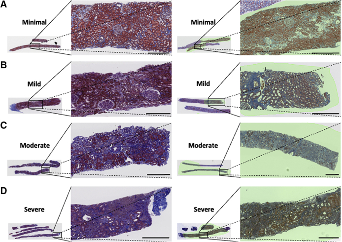
Trichrome-stained whole-slide images of human renal biopsies. Sample trichrome images are shown on cases graded as minimal interstitial fibrosis and tubular atrophy (IFTA; A), mild IFTA (B), moderate IFTA (C), and severe IFTA (D). For each grade, two different images are shown. Left panels: Images had no annotations because the entire image was composed of the cortical region. Right panels: On the images, a nephropathologist (C.A.C.) annotated the cortical regions. For cases with no annotations, the entire image served as inputs to the deep-learning (DL) model; and for cases with annotations, the annotated regions were segmented, which served as inputs to the DL model. The final IFTA grading was derived by performing majority voting on the ratings obtained from five nephropathologists. Scale bars = 400 μm (A–D).

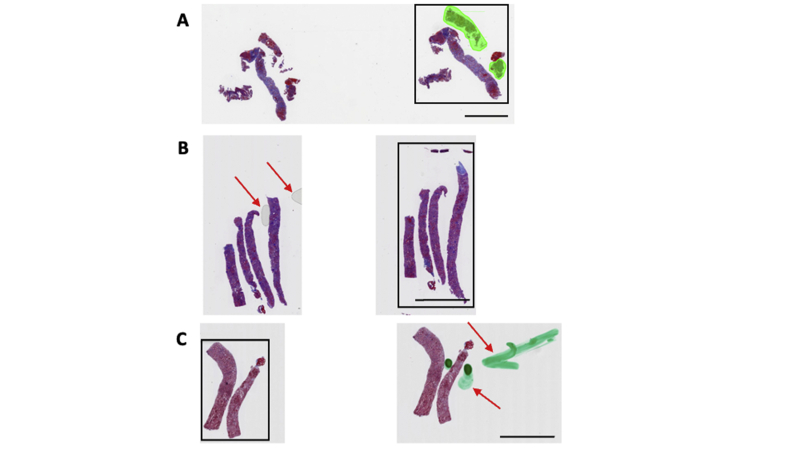
A manual quality check was performed on all the WSIs by a nephropathologist (C.A.C.). This check ensured there were no artifacts on the selected WSI regions, such as air bubbles, folding, compressing, tearing, overstaining or understaining, stain batch variations, knife chatter, and thickness variances. Because most WSIs had multiple cores, the nephropathologist was able to select a core that had no quality issues on all cases (Supplemental Figure S2). The selected portion of the WSI was then carefully cropped and converted to numeric matrices for further analysis.

Fibrosis Grading

A nephropathologist (C.A.C.) identified and annotated the cortical regions within each WSI (Figure 1) where both cortex and medulla were present. All the nephropathologists accessed and independently reviewed the WSIs for IFTA using PixelView on a web browser from their respective computers. The score was provided as percentage of cortical regions with IFTA (0% to 100%), which was then converted to a semiquantitative grade: ≤10% (none or minimal), 11% to 25% (mild), 26% to 50% (moderate), and >50% (severe).¹⁹ The final IFTA grades were computed by performing majority voting on the grades obtained from each nephropathologist. The fibrosis scores for the KPMP data set were obtained directly from the study investigators and converted to IFTA grades using the same criterion. The derived IFTA grades from both data sets were used for further analysis.

Deep-Learning Framework

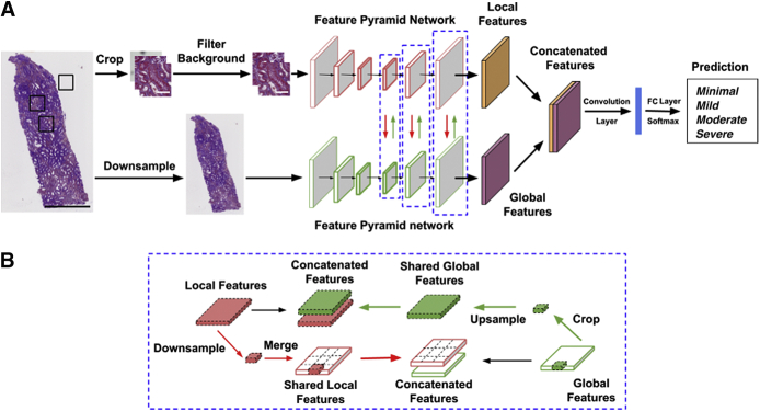
Our DL architecture is based on combining the features learned at the global level of the WSI along with the ones learned from local high-resolution image patches from the WSI (Figure 2A). Similar DL architectures have been recently applied to computer vision-related tasks.20, 21, 22, 23, 24 This architecture is referred to as glpathnet. Briefly, glpathnet comprises three arms: i) local branch (Figure 2A), ii) global branch (Figure 2A), and iii) ensemble branch (Figure 2A). The local branch receives cropped filtered patches from the original images as the input to a Feature Pyramid Network (FPN) model.²⁵ The FPN uses an efficient architecture to leverage multiple feature maps at low and high resolutions to detect objects at different scales.

Figure 2.

Deep-learning architecture. A: The proposed deep neural network uses a novel approach that learns from both local and global image features to predict the output label of interest. The local features are learned at the level of image patches, and the global features are learned on a downsampled version of the whole image. The local and global feature maps are fused at each layer, where each layer is highlighted using a blue dashed boxed area. The black boxed areas on the whole-slide image (far left) denote the locations where image patches are extracted for further processing. B: A schematic representing local and global feature sharing is shown. Scale bars: 800 μm (A, black); 50 μm (A, white).

Cropped image patches (N_p × N_p pixels) were automatically extracted from the original WSIs and labeled as tissue or background using the following criterion. Image patches containing tissue within at least 50% or more pixels were labeled as tissue and otherwise labeled as background. The local branch containing the image patches labeled as tissue was fed into the FPN model. The global branch containing downsampled low-resolution versions (N_g × N_g pixels) of the original WSIs served as inputs to another FPN model. To enable local and global feature interaction, the feature maps from all layers of either branches were shared with the others (Figure 2B). The global branch cropped its feature maps at the same spatial location as the current local patch. To interact with the local branch, glpathnet upsamples the cropped feature maps to the same size of the feature maps from the local branch in the layer with the same depth. Subsequently, glpathnet concatenates the local feature maps and cropped global feature maps, which are fed into the next layer in the local branch. In a symmetrical manner, the local branch downsamples its feature maps to the same relative spatial ratio as the patches cropped from the original input image. On the basis of the location of the cropped patches, the downsampled local feature maps are merged together into feature maps of the same size of the global branch feature in the same layer. Feature maps with all zeros were used for the patches labeled as background. The global feature maps and merged local feature maps were concatenated and fed into the next layer in the global branch.

The ensemble branch in glpathnet contains a convolutional layer, followed by a fully connected layer. It takes the concatenated feature maps from the last layer of the local branch and the same ones from the global branch. The output of the ensemble branch is a patch-level IFTA grade, and the final IFTA grade was determined as the most common patch-level IFTA grade.

Cross-entropy loss was used to train glpathnet on the OSUWMC data using a pretrained DL architecture (ResNet50),²⁶ as part of the convolutional network of the FPN model. To maximize efficiency, both N_p and N_g were set to 508 pixels. Adam optimizer (β₁ = 0.9; β₂ = 0.999) was used to optimize model training with a batch size of 6. We assigned the initial learning rate to 2 × 10⁻⁵ for the local branch and 1 × 10⁻⁴ for the global branch. Glpathnet was implemented using PyTorch, and model training was performed on a graphical processing unit (GPU) workstation containing GeForce RTX 2080 Ti graphics cards (NVIDIA, Santa Clara, CA) with an 11-Gb GDDR6 memory. Model training took <16 hours to reach convergence. Prediction of IFTA grade on a new WSI that was not used for model training took approximately 30 seconds.

Traditional Machine-Learning Model

For comparison, an IFTA classification model was constructed based on traditional machine learning that used derived features from OSUWMC WSI data. Weighted neighbor distance was used that included compound hierarchy of algorithms representing morphology,27, 28, 29 which is a multipurpose image classifier that can extract approximately 3000 generic image descriptors, including polynomial decompositions, high-contrast features, pixel statistics, and textures (Supplemental Table S2). These features were directly derived from the raw WSI, transforms of the WSI, and compound transforms of the WSI (transforms of transforms). Using these features as inputs, a four-label classifier was constructed to predict the final IFTA grade. The model was trained on the OSUWMC data set, and the KPMP data set was used for testing.

Performance Metrics

The final IFTA grade (reference estimate) was determined by taking the majority vote on the IFTA grading among all the five nephropathologists. The agreement between the nephropathologists was computed using κ scores between each pathologist grade and the reference estimate. The percentage agreement between the pathologists and between pathologists and the reference estimate was also computed. For the DL model trained on the OSUWMC data set, a fivefold cross validation was performed, and the average model accuracy, sensitivity/recall, specificity, precision, and κ scores were reported. Sensitivity/recall measures the proportion of true positives that are correctly identified, specificity measures the proportion of true negatives that are correctly identified, and precision is a fraction of true positives over the total number of positive calls.

Data Sharing

Computer scripts and manuals are made available on GitHub (https://github.com/vkola-lab/ajpa2021, last accessed May 1, 2021). Data from the OSUWMC can be obtained on request and subject to institutional approval. Data from KPMP can be freely downloaded (https://atlas.kpmp.org/repository, last accessed May 1, 2021).

Informed Consent

Informed consent was not required as all obtained data were de-identified.

Results

There was good agreement on the IFTA grading between the nephropathologists, where pairwise agreements ranged from 0.48 to 0.63 (Figure 3A). Interpathologist ratings assessed using pairwise κ showed moderate agreement, ranging from 0.31 to 0.50 (Figure 3B). There was good agreement when each pathologist grading was compared with the reference IFTA grade (κ = 0.622 ± 0.071). Note that this agreement must be interpreted by considering the evidence that the reference IFTA grade was also derived from the pathologists' grades.

Figure 3.

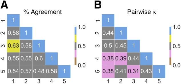
Pathologist-level interstitial fibrosis and tubular atrophy grading. A: Pairwise values of percentage agreement between the nephropathologists are shown on the cases obtained from The Ohio State University Wexner Medical Center (OSUWMC). The values were normalized to lie between 0 and 1. B: Pairwise κ scores between the nephropathologists on the OSUWMC data are shown. The κ values range from 0 to 1, where 0 indicates no agreement and 1 indicates perfect agreement.

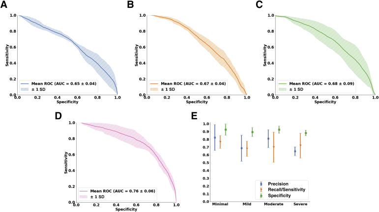
The DL model (glpathnet) accurately predicted the IFTA grade on the OSUWMC data (accuracy = 71.8% ± 5.3%), based on fivefold cross validation (Figure 4). The patch-level model predictions also consistently predicted IFTA grade, as indicated by the class-level receiver operating characteristic (ROC) curves (Figure 4, A–D). For the minimal IFTA label, the patch-level cross-validated model resulted in area under ROC curve of 0.65 ± 0.04. For the mild IFTA label, the area under ROC curve was 0.67 ± 0.04; for the moderate IFTA label, the area under ROC curve was 0.68 ± 0.09; and for the severe IFTA label, the area under ROC curve was 0.76 ± 0.06. For each class label, the cross-validated model performance on the WSIs was evaluated by computing mean precision, mean sensitivity, and mean specificity along with their respective standard deviations Figure 4E). For the minimal IFTA label, the precision was 0.82 ± 0.17, the sensitivity was 0.77 ± 0.08, and the specificity was 0.93 ± 0.07. For the mild IFTA label, the precision was 0.71 ± 0.15, the sensitivity was 0.68 ± 0.10, and the specificity was 0.91 ± 0.05. For the moderate IFTA label, the precision was 0.82 ± 0.10, the sensitivity was 0.73 ± 0.20, and the specificity was 0.93 ± 0.05. Finally, for the severe IFTA label, the precision was 0.65 ± 0.06, the sensitivity was 0.72 ± 0.16, and the specificity was 0.88 ± 0.04. Because of the nature by which specificity was computed for the model (ie, minimal versus not minimal, mild versus not mild, moderate versus not moderate, and severe versus not severe), the values were generally higher than precision and sensitivity for all cases.

Figure 4.

Deep-learning model performance on The Ohio State University Wexner Medical Center data set. A–D: Patch-level performance of the fivefold cross-validated model is shown for each interstitial fibrosis and tubular atrophy (IFTA) grade. A: The receiver operating characteristic (ROC) curve for the minimal grade is shown. B: The ROC curve for the mild grade is shown. C and D: The ROC curves for moderate and severe grades, respectively, are shown. E: Model performance, including precision, sensitivity, and specificity on the entire whole-slide images, is shown for each IFTA grade. AUC, area under ROC curve.

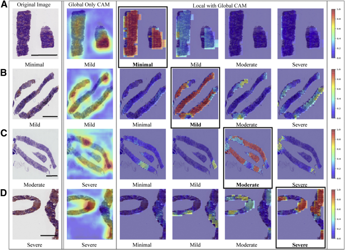
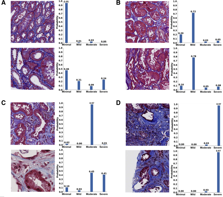
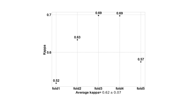
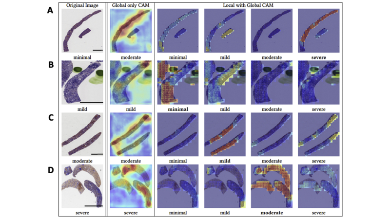
Fivefold cross validation indicated good agreement between the true and predicted IFTA grades on the OSUWMC data (κ = 0.62 ± 0.07) (Supplemental Figure S3). Class activation mapping (CAM) was performed on the WSIs to explore the regions that are highly associated with the output class label (Figure 5 and Supplemental Figure S4). Two different strategies were used to generate CAMs. The first method generated CAMs at the WSI (or global) level without utilizing the local features, whereas the second method generated CAMs that synthesized features at the local and global level. Although both these strategies generated CAMs that highlighted image subregions, CAMs based on the model that combined local and global representations showed higher qualitative association with the output label. Patch-level probabilities with high-degree association with the IFTA grade were generated (Figure 6). Each image patch and its set of probability values were reviewed by the nephropathologist (C.A.C.), who confirmed that patch-level patterns were consistent with model predictions of the corresponding IFTA grades. Note that C.A.C. reviewed the patch-based results after they performed IFTA grading on all the WSIs, and were not biased by the model results during IFTA grading. It should be noted that the IFTA grade was based on WSI-level estimation, and the probabilities were predicted at patch level.

Figure 5.

Visualization of discriminatory regions within the pathology images. The first column represents the original whole-slide images (WSIs) along with the ground truth labels derived using majority voting on the pathologists' interstitial fibrosis and tubular atrophy (IFTA) grades. The second column shows global class activation maps (CAMs) generated on the entire WSI and the global CAM-based model predictions. The third to sixth columns show CAMs derived by combining local and global representations for each class label along with their corresponding model predictions. The CAM indicating the correct prediction is indicated with a black border around it. A: In the first row, a case with a minimal IFTA grade is shown. The approach that used global CAMs only predicted the IFTA grade as mild, whereas the approach using local and global CAMs correctly predicted the IFTA grade as minimal. B: In the second row, a case with a mild IFTA grade is shown. Both the approaches that used global CAMs only and the one that used local and global CAMs correctly predicted the IFTA grade as mild. C: In the third row, a case with a moderate IFTA grade is shown. The approach that used global CAMs only predicted the IFTA grade as severe, whereas the approach using local and global CAMs correctly predicted the IFTA grade as moderate. D: In the fourth row, a case with a severe IFTA grade is shown. Both the approaches that used global CAMs only and the one that used local and global CAMs correctly predicted the IFTA grade as severe. All these cases were obtained from The Ohio State University Wexner Medical Center. Scale bars = 1300 μm (A–D).

Figure 6.

Patch-level probabilities of the deep-learning model. Selected image patches and their corresponding probability values for each interstitial fibrosis and tubular atrophy (IFTA) grade are shown. A: The set of image patches shows the ones with minimal IFTA. B: The patches indicate the ones with mild IFTA. C: The cases show image patches with moderate IFTA. D: The image patches indicate the cases with severe IFTA. All the image patches and their corresponding probability values were reviewed by a nephropathologist (C.A.C.). All patches are of the same scale. Scale bars = 50 μm (A–D).

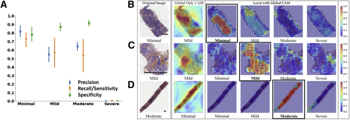
Although the fivefold cross-validated model on the OSUWMC data set generated convincing results, performance of glpathnet on an external data set was also evaluated. The cross-validated model was used to predict IFTA grade on the KPMP data. The entire process, including random data split followed by model training using OSUWMC data and prediction on KPMP data, was repeated five times, and average model performance was reported (accuracy = 65.0% ± 4.2%) (Figure 7A). Also, for each class label, the cross-validated model performance on the WSIs was evaluated by computing mean precision, mean sensitivity, and mean specificity along with their respective SDs. For the minimal IFTA label, the precision was 0.82 ± 0.06, the sensitivity was 0.73 ± 0.08, and the specificity was 0.78 ± 0.08. For the mild IFTA label, the precision was 0.55 ± 0.08, the sensitivity was 0.57 ± 0.17, and the specificity was 0.87 ± 0.04. For the moderate IFTA label, the precision was 0.64 ± 0.05, the sensitivity was 0.53 ± 0.19, and the specificity was 0.92 ± 0.03. Performance scores for the severe IFTA label were not computed because none of the cases from the KPMP data set was graded as severe IFTA. Even for those cases, CAMs based on the model that combined local and global representations had a better association with the output label (Figure 7, B–D). Model performance between these cohorts featuring broad variance in slide staining protocols, slide digitization, geographic location, and recruitment criteria suggests a good degree of generalizability. Moreover, sensitivity analysis on the model parameters revealed that the selected model configuration resulted in best performance on both the OSUWMC and the KPMP data sets (Supplemental Table S3). Of note, the DL model outperformed the traditional machine-learning model (weighted neighbor distance using compound hierarchy of algorithms representing morphology), which was constructed using generic image descriptors from the WSIs. Specifically, weighted neighbor distance using compound hierarchy of algorithms representing morphology achieved an accuracy of 21.4% ± 7.5% on the OSUWMC data set (Table 3) and an accuracy of 35.0% ± 14.7% on the KPMP data set (Table 4). Taken together, these findings underline the advantage of utilizing DL for predicting IFTA grade on digitized kidney biopsies.

Figure 7.

Deep-learning model performance on the Kidney Precision Medicine Project data set. A: Model performance, including precision, sensitivity, and specificity on the entire whole-slide images (WSIs), is shown for each interstitial fibrosis and tubular atrophy (IFTA) grade. Note that performance scores for the severe IFTA label were not computed because none of the cases was graded as severe IFTA. B–D: Class activation maps (CAMs) were generated on the data set. The first column represents the original WSIs along with the ground truth labels derived using majority voting on the pathologists' IFTA grades. The second column shows global CAMs generated on the entire WSI and the global CAM-based model predictions. The third to sixth columns show CAMs derived by combining local and global representations for each class label along with their corresponding model predictions. The CAM indicating the correct prediction is indicated with a black border around it. B: In the first row, a case with a minimal IFTA grade is shown. The approach that used global CAMs only predicted the IFTA grade as mild, whereas the approach using local and global CAMs correctly predicted the IFTA grade as minimal. C: In the second row, a case with a mild IFTA grade is shown. Both the approaches that used global CAMs only and the one that used local and global CAMs correctly predicted the IFTA grade as mild. D: In the third row, a case with a moderate IFTA grade is shown. The approach that used global CAMs only predicted the IFTA grade as minimal, whereas the approach using local and global CAMs correctly predicted the IFTA grade as moderate. n = 28 (A). Scale bar = 400 μm (B–D).

Table 3.

Performance of the Traditional Machine-Learning Model on The Ohio State University Wexner Medical Center Data Set

Description	Minimal	Mild	Moderate	Severe
Precision	0.12 ± 0.15	0.25 ± 0.13	0.22 ± 0.12	0.29 ± 0.18
Recall/sensitivity	0.10 ± 0.13	0.40 ± 0.17	0.27 ± 0.13	0.23 ± 0.17
Specificity	0.89 ± 0.09	0.59 ± 0.14	0.67 ± 0.12	0.86 ± 0.07

A machine-learning model based on weighted neighbor distance using compound hierarchy of algorithms representing morphology was constructed by deriving approximately 3000 features from the whole-slide image data obtained from The Ohio State University Wexner Medical Center to predict interstitial fibrosis and tubular atrophy grade. The trained model was then used to predict on the data obtained from the Kidney Precision Medicine Project. Performance of the model after fivefold cross validation on The Ohio State University Wexner Medical Center data set is shown. Data are expressed as means SD.

Table 4.

Performance of the Traditional Machine-Learning Model on the Kidney Precision Medicine Project

Description	Minimal	Mild	Moderate	Severe
Precision	0.52 ± 0.26	0.30 ± 0.40	0.26 ± 0.20	N/A
Recall/sensitivity	0.49 ± 0.30	0.07 ± 0.08	0.27 ± 0.20	N/A
Specificity	0.63 ± 0.24	0.88 ± 0.17	0.79 ± 0.23	N/A

The trained model based on weighted neighbor distance using compound hierarchy of algorithms representing morphology on The Ohio State University Wexner Medical Center data set was used to predict on the data obtained from the Kidney Precision Medicine Project. Performance of the trained model on the Kidney Precision Medicine Project data set is shown. Data are expressed as means SD.

N/A, not available.

Discussion

We developed a deep-learning framework that can analyze digitized kidney biopsies at the level of an expert pathologist. Specifically, we selected automated IFTA grading as our task because fibrosis on kidney biopsy is a known structural correlate of progressive and chronic kidney disease.^19,30 Despite knowing the putative link between IFTA grade and disease prognosis, there remains uncertainty on how to best measure fibrosis within the kidney. Farris and Alpers² provided an interesting perspective on this aspect in their recent article, where they argue that current analytic approaches generally avoid rigorous assessment of various aspects related to characterizing fibrosis of the tubulointerstitium. They note that human reproducibility is not generally high because there is no agreeable definition on how to measure IFTA. For example, some consider percentage interstitial fibrosis to be percentage of overall tissue occupied by fibrous tissue, whereas others note the percentage of fibrosis to be the percentage of abnormal tissue. In clinical practice, however, people often refer to scoring systems defined by established national and international working groups (Renal Pathology Society Working Group or Banff classification) for grading fibrosis. Morphometric analysis can also be performed to evaluate renal fibrosis as this approach can bring efficiency, reproducibility, and functional correlation.³ These developments lend themselves to using more advanced computer methods, such as machine learning on digitized images for IFTA grading.

The novelty of glpathnet is underlined by the fact that it combines local representations to quantify features at the image patch level as well as at the WSI level to accurately predict the IFTA grade. A combination of both these assessments provides a comprehensive evaluation of IFTA. This method appears to capture the typical workflow of pathologists as they examine the WSIs by performing manual operations, such as panning across the WSI to perceive the overall context, zooming in and out of specific WSI regions to evaluate the local pathology, and finally combining the information learned from both these steps to determine the IFTA grade. We must, however, acknowledge that the nephropathologist's clinical impression and diagnosis is based on contextual factors above and beyond visual inspection of a lesion in isolation. Nevertheless, by identifying WSI regions using CAMs that are highly indicative of a class label, this approach provides a quantitative basis by which to interpret the model-based predictions rather than viewing DL methods as black-box approaches. As such, this approach stands in contrast to other methods that rely on expert-driven annotations and segmentation algorithms that attempt to quantify histologic regions and derive information for pathologic assessment.^12,15, 16, 17, 18

Saliency mapping based on CAMs is increasingly being considered as a framework to generate visual interpretations of model predictions by highlighting image subregions that are presumably correlated with the outputs of interest.31, 32, 33, 34, 35, 36, 37, 38, 39, 40 These heat maps can be generated for any input image that is associated with an output class label (ie, IFTA grade). The underlying assumption is that the heat map representation highlights pixels of the image that trigger the model to associate the image with a particular class label. Our DL strategy that combined local and global representations consistently predicted the correct IFTA grade and generated interpretable CAMs. This strategy turned out to be superior than using only the global representations because several image subregions highlighted by glpathnet-derived CAMs appear to have high correlation with the output class label.

The morphologic assessment of interstitial fibrosis and tubular atrophy by renal core biopsy has inherent limitations that cannot be circumvented by the current work. Renal biopsy samples are in general obtained from limited regions of the kidney that are most accessible via imaging-guided percutaneous biopsy. As such, a renal core biopsy comprises only a small percentage of the overall kidney mass and may not be completely representative of the kidney as a whole, especially in disease processes with irregular distribution throughout the parenchyma, leading to focal scarring. Nevertheless, for most disease processes involving the kidney, the degree of IFTA as estimated by renal core biopsies has been shown to be one of the strongest morphologic predictors of prognosis, which is why it continues to be an important part of the renal biopsy report.¹⁹ Thus, any tool that can facilitate IFTA assessment and increase its consistency across pathology services is valuable not only to the pathologists but also to the clinicians because it provides a more robust prognostic marker that could help guide patient management.

This study has a few limitations. First is the sole reliance on WSIs derived using the trichrome stain, as this is commonly used by nephropathologists. Past studies have found that trichrome-stained slides can produce cost-effective, efficient, reproducible, and functional correlations with outcomes, such as estimated glomerular filtration rate.^2,3 Some pathologists, however, rely on other protocols, such as hematoxylin and eosin, periodic acid–Schiff, Jones methenamine silver, or Sirius Red staining, to grade fibrosis.^2,41, 42, 43 Also, this DL framework has the potential to be applied effectively to WSIs generated with other staining protocols. The OSUWMC cases included in-house cases and consults from external institutions, indicating that this model performed well on cases that may have employed different staining techniques. Furthermore, this DL framework provides an automated approach to IFTA grading to assist the pathologist rather than replacing the human factor. Nevertheless, the ability to classify WSIs using a computer with the accuracy of an experienced nephropathologist has the potential to inform pathology practices, especially in resource-limited settings.

In conclusion, we demonstrated the effectiveness of capturing localized morphologic along with WSI-level contextual features using an advanced DL architecture (glpathnet) to mimic the pathologist's approach to IFTA grading. It is possible to use glpathnet to study other organ-specific pathologies focused on evaluating fibrosis, as well as WSIs generated using other histologic staining protocols. This proposed framework to local and contextual IFTA grading can serve as an analysis template for researchers and practitioners when new data from cohort studies, such as KPMP, become available. Such methods may hold the potential to generate more reproducible IFTA readings (eg, in multicenter studies) than readings by nephropathologists. Further validation of the glpathnet across different pathology practices and patient populations is necessary to study its efficacy across the full distribution and spectrum of fibrotic lesions.

Supplemental Data

Supplemental Figure S1.

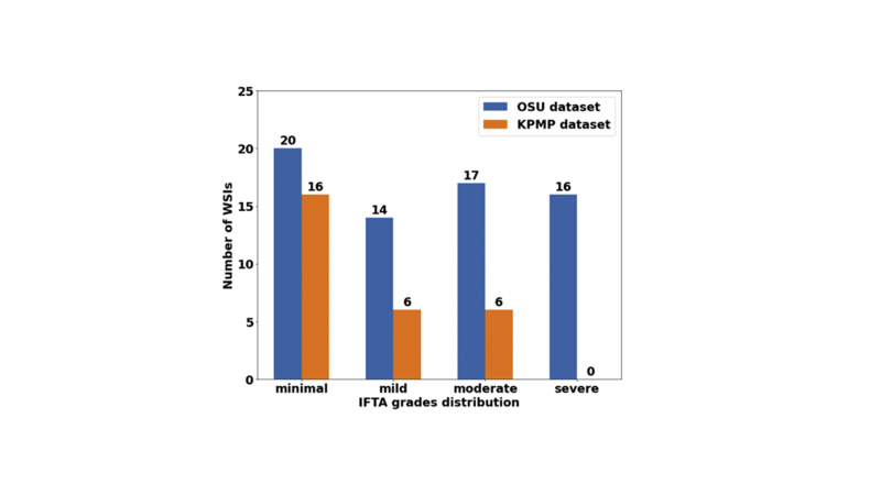
Whole-slide image (WSI) distribution. Numbers of WSIs per interstitial fibrosis and tubular atrophy (IFTA) grade in The Ohio State University (OSU) Wexner Medical Center and Kidney Precision Medicine Project (KPMP) data sets are shown.

Supplemental Figure S2.

Quality check and region of interest selection. A manual quality check was performed by a nephropathologist to identify and select whole-slide image regions that served as inputs to the deep-learning model. A: In this case, the core on the extreme right, containing both the cortex and the medulla, was selected for further analysis. B: This case shows the presence of air bubbles (red arrows) on the second core. The third core was selected for further analysis. C: This case shows staining artifacts (red arrows) on the second core. The first core was selected for further analysis. Scale bar = 3000 μm (A–C).

Supplemental Figure S3.

Model agreement with the ground truth. Fivefold cross validation was performed on The Ohio State University Wexner Medical Center data set to evaluate the deep-learning model. For each fold, κ was computed to evaluate the agreement of the model with the ground truth, defined using majority voting on the interstitial fibrosis and tubular atrophy grading performed by the nephropathologists.

Supplemental Figure S4.

Visualization of discriminatory regions within the pathology images. The first column represents the original whole-slide images (WSIs) along with the ground truth labels derived using majority voting on the pathologists' interstitial fibrosis and tubular atrophy (IFTA) grades. The second column shows global class activation maps (CAMs) generated on the entire WSI and the global CAM-based model predictions. The third to sixth columns show CAMs derived by combining local and global representations for each class label along with their corresponding model predictions. A: In the first row, a case with a minimal IFTA grade is shown. The approach that used global CAMs only predicted the IFTA grade as moderate, whereas the approach using local and global CAMs predicted the IFTA grade as severe. B: In the second row, a case with a mild IFTA grade is shown. In this case, the global only CAM-based model correctly predicted the IFTA grade, whereas the local and global CAM-based approach predicted the IFTA grade as minimal. C: In the third row, a case with a moderate IFTA grade is shown. The approach that used global CAMs only correctly predicted the IFTA grade as moderate, whereas the approach using local and global CAMs incorrectly predicted the IFTA grade as mild. D: In the fourth row, a case with a severe IFTA grade is shown. The approach that used global CAMs only correctly predicted the IFTA grade as severe, whereas the approach using local and global CAMs correctly predicted the IFTA grade as moderate. All these cases were obtained from The Ohio State University Wexner Medical Center. Scale bar = 1300 μm (A–D).

References

- 1.Amann K., Haas C.S. What you should know about the work-up of a renal biopsy. Nephrol Dial Transpl. 2006;21:1157–1161. doi: 10.1093/ndt/gfk037. [DOI] [PubMed] [Google Scholar]
- 2.Farris A.B., Alpers C.E. What is the best way to measure renal fibrosis?: a pathologist's perspective. Kidney Int Suppl (2011) 2014;4:9–15. doi: 10.1038/kisup.2014.3. [DOI] [PMC free article] [PubMed] [Google Scholar]
- 3.Farris A.B., Adams C.D., Brousaides N., Della Pelle P.A., Collins A.B., Moradi E., Smith R.N., Grimm P.C., Colvin R.B. Morphometric and visual evaluation of fibrosis in renal biopsies. J Am Soc Nephrol. 2011;22:176–186. doi: 10.1681/ASN.2009091005. [DOI] [PMC free article] [PubMed] [Google Scholar]
- 4.Becker J.U., Mayerich D., Padmanabhan M., Barratt J., Ernst A., Boor P., Cicalese P.A., Mohan C., Nguyen H.V., Roysam B. Artificial intelligence and machine learning in nephropathology. Kidney Int. 2020;98:65–75. doi: 10.1016/j.kint.2020.02.027. [DOI] [PMC free article] [PubMed] [Google Scholar]
- 5.Barisoni L., Lafata K.J., Hewitt S.M., Madabhushi A., Balis U.G.J. Digital pathology and computational image analysis in nephropathology. Nat Rev Nephrol. 2020;16:669–685. doi: 10.1038/s41581-020-0321-6. [DOI] [PMC free article] [PubMed] [Google Scholar]
- 6.Sealfon R.S.G., Mariani L.H., Kretzler M., Troyanskaya O.G. Machine learning, the kidney, and genotype-phenotype analysis. Kidney Int. 2020;97:1141–1149. doi: 10.1016/j.kint.2020.02.028. [DOI] [PMC free article] [PubMed] [Google Scholar]
- 7.Saez-Rodriguez J., Rinschen M.M., Floege J., Kramann R. Big science and big data in nephrology. Kidney Int. 2019;95:1326–1337. doi: 10.1016/j.kint.2018.11.048. [DOI] [PubMed] [Google Scholar]
- 8.Niel O., Bastard P. Artificial intelligence in nephrology: core concepts, clinical applications, and perspectives. Am J Kidney Dis. 2019;74:803–810. doi: 10.1053/j.ajkd.2019.05.020. [DOI] [PubMed] [Google Scholar]
- 9.Santo B.A., Rosenberg A.Z., Sarder P. Artificial intelligence driven next-generation renal histomorphometry. Curr Opin Nephrol Hypertens. 2020;29:265–272. doi: 10.1097/MNH.0000000000000598. [DOI] [PMC free article] [PubMed] [Google Scholar]
- 10.Kannan S., Morgan L.A., Liang B., Cheung M.G., Lin C.Q., Mun D., Nader R.G., Belghasem M.E., Henderson J.M., Francis J.M., Chitalia V.C., Kolachalama V.B. Segmentation of glomeruli within trichrome images using deep learning. Kidney Int Rep. 2019;4:955–962. doi: 10.1016/j.ekir.2019.04.008. [DOI] [PMC free article] [PubMed] [Google Scholar]
- 11.Kolachalama V.B., Singh P., Lin C.Q., Mun D., Belghasem M.E., Henderson J.M., Francis J.M., Salant D.J., Chitalia V.C. Association of pathological fibrosis with renal survival using deep neural networks. Kidney Int Rep. 2018;3:464–475. doi: 10.1016/j.ekir.2017.11.002. [DOI] [PMC free article] [PubMed] [Google Scholar]
- 12.Marsh J.N., Matlock M.K., Kudose S., Liu T.C., Stappenbeck T.S., Gaut J.P., Swamidass S.J. Deep learning global glomerulosclerosis in transplant kidney frozen sections. IEEE Trans Med Imaging. 2018;37:2718–2728. doi: 10.1109/TMI.2018.2851150. [DOI] [PMC free article] [PubMed] [Google Scholar]
- 13.Chagas P., Souza L., Araujo I., Aldeman N., Duarte A., Angelo M., Dos-Santos W.L.C., Oliveira L. Classification of glomerular hypercellularity using convolutional features and support vector machine. Artif Intell Med. 2020;103:101808. doi: 10.1016/j.artmed.2020.101808. [DOI] [PubMed] [Google Scholar]
- 14.Hermsen M., de Bel T., den Boer M., Steenbergen E.J., Kers J., Florquin S., Roelofs J., Stegall M.D., Alexander M.P., Smith B.H., Smeets B., Hilbrands L.B., van der Laak J. Deep learning-based histopathologic assessment of kidney tissue. J Am Soc Nephrol. 2019;30:1968–1979. doi: 10.1681/ASN.2019020144. [DOI] [PMC free article] [PubMed] [Google Scholar]
- 15.Jayapandian C.P., Chen Y., Janowczyk A.R., Palmer M.B., Cassol C.A., Sekulic M., Hodgin J.B., Zee J., Hewitt S.M., O'Toole J., Toro P., Sedor J.R., Barisoni L., Madabhushi A. Development and evaluation of deep learning-based segmentation of histologic structures in the kidney cortex with multiple histologic stains. Kidney Int. 2020;99:86–101. doi: 10.1016/j.kint.2020.07.044. [DOI] [PMC free article] [PubMed] [Google Scholar]
- 16.Uchino E., Suzuki K., Sato N., Kojima R., Tamada Y., Hiragi S., Yokoi H., Yugami N., Minamiguchi S., Haga H., Yanagita M., Okuno Y. Classification of glomerular pathological findings using deep learning and nephrologist-AI collective intelligence approach. Int J Med Inform. 2020;141:104231. doi: 10.1016/j.ijmedinf.2020.104231. [DOI] [PubMed] [Google Scholar]
- 17.Ginley B., Lutnick B., Jen K.Y., Fogo A.B., Jain S., Rosenberg A., Walavalkar V., Wilding G., Tomaszewski J.E., Yacoub R., Rossi G.M., Sarder P. Computational segmentation and classification of diabetic glomerulosclerosis. J Am Soc Nephrol. 2019;30:1953–1967. doi: 10.1681/ASN.2018121259. [DOI] [PMC free article] [PubMed] [Google Scholar]
- 18.Bouteldja N., Klinkhammer B.M., Bulow R.D., Droste P., Otten S.W., Freifrau von Stillfried S., Moellmann J., Sheehan S.M., Korstanje R., Menzel S., Bankhead P., Mietsch M., Drummer C., Lehrke M., Kramann R., Floege J., Boor P., Merhof D. Deep learning-based segmentation and quantification in experimental kidney histopathology. J Am Soc Nephrol. 2021;32:52–68. doi: 10.1681/ASN.2020050597. [DOI] [PMC free article] [PubMed] [Google Scholar]
- 19.Srivastava A., Palsson R., Kaze A.D., Chen M.E., Palacios P., Sabbisetti V., Betensky R.A., Steinman T.I., Thadhani R.I., McMahon G.M., Stillman I.E., Rennke H.G., Waikar S.S. The prognostic value of histopathologic lesions in native kidney biopsy specimens: results from the Boston Kidney Biopsy Cohort Study. J Am Soc Nephrol. 2018;29:2213–2224. doi: 10.1681/ASN.2017121260. [DOI] [PMC free article] [PubMed] [Google Scholar]
- 20.Chen W., Jiang Z., Wang Z., Cui K., Qian X. 2019. Collaborative Global-Local Networks for Memory-Efficient Segmentation of Ultra-High Resolution Images. Proceedings of the IEEE/CVF Conference on Computer Vision and Pattern Recognition (CVPR) pp. 8924–8933. . Long Beach, CA. [Google Scholar]
- 21.Lin C.Y., Chiu Y.C., Ng H.F., Shih T.K., Lin K.H. Global-and-local context network for semantic segmentation of street view images. Sensors (Basel) 2020;20:2907. doi: 10.3390/s20102907. [DOI] [PMC free article] [PubMed] [Google Scholar]
- 22.Wang S., Ye Z., Wang Y. 2018. GLNet for Target Detection in Millimeter Wave Images. Proceedings of the 3rd International Conference on Multimedia and Image Processing - ICMIP 2018; pp. 12–16. [Google Scholar]
- 23.Wu T., Lei Z., Lin B., Li C., Qu Y., Xie Y. Patch proposal network for fast semantic segmentation of high-resolution images. Proc AAAI Conf Artif Intelligence. 2020;34:12402–12409. [Google Scholar]
- 24.Zhang S., Song L., Gao C., Sang N. GLNet: global local network for weakly supervised action localization. IEEE Trans Multimedia. 2020;22:2610–2622. [Google Scholar]
- 25.Lin T.-Y., Dollár P., Girshick R.B., He K., Hariharan B., Belongie S.J. IEEE Computer Society; Honolulu, HI: 2017. Feature Pyramid Networks for Object Detection: Computer Vision and Pattern Recognition; pp. 936–944. [Google Scholar]
- 26.He K., Zhang X., Ren S., Sun J. 2016. Deep Residual Learning for Image Recognition. 2016 IEEE Conference on Computer Vision and Pattern Recognition (CVPR) pp. 770–778. [Google Scholar]
- 27.Orlov N., Shamir L., Macura T., Johnston J., Eckley D.M., Goldberg I.G. WND-CHARM: multi-purpose image classification using compound image transforms. Pattern Recognit Lett. 2008;29:1684–1693. doi: 10.1016/j.patrec.2008.04.013. [DOI] [PMC free article] [PubMed] [Google Scholar]
- 28.Shamir L., Orlov N., Eckley D.M., Macura T., Johnston J., Goldberg I.G. Wndchrm - an open source utility for biological image analysis. Source Code Biol Med. 2008;3:13. doi: 10.1186/1751-0473-3-13. [DOI] [PMC free article] [PubMed] [Google Scholar]
- 29.Shamir L., Delaney J.D., Orlov N., Eckley D.M., Goldberg I.G. Pattern recognition software and techniques for biological image analysis. PLoS Comput Biol. 2010;6:e1000974. doi: 10.1371/journal.pcbi.1000974. [DOI] [PMC free article] [PubMed] [Google Scholar]
- 30.Mariani L.H., Martini S., Barisoni L., Canetta P.A., Troost J.P., Hodgin J.B., Palmer M., Rosenberg A.Z., Lemley K.V., Chien H.P., Zee J., Smith A., Appel G.B., Trachtman H., Hewitt S.M., Kretzler M., Bagnasco S.M. Interstitial fibrosis scored on whole-slide digital imaging of kidney biopsies is a predictor of outcome in proteinuric glomerulopathies. Nephrol Dial Transplant. 2018;33:310–318. doi: 10.1093/ndt/gfw443. [DOI] [PMC free article] [PubMed] [Google Scholar]
- 31.Chang G.H., Felson D.T., Qiu S., Guermazi A., Capellini T.D., Kolachalama V.B. Assessment of knee pain from MR imaging using a convolutional Siamese network. Eur Radiol. 2020;30:3538–3548. doi: 10.1007/s00330-020-06658-3. [DOI] [PMC free article] [PubMed] [Google Scholar]
- 32.Bien N., Rajpurkar P., Ball R.L., Irvin J., Park A., Jones E., Bereket M., Patel B.N., Yeom K.W., Shpanskaya K., Halabi S., Zucker E., Fanton G., Amanatullah D.F., Beaulieu C.F., Riley G.M., Stewart R.J., Blankenberg F.G., Larson D.B., Jones R.H., Langlotz C.P., Ng A.Y., Lungren M.P. Deep-learning-assisted diagnosis for knee magnetic resonance imaging: development and retrospective validation of MRNet. PLoS Med. 2018;15:e1002699. doi: 10.1371/journal.pmed.1002699. [DOI] [PMC free article] [PubMed] [Google Scholar]
- 33.Cai J., Xing F., Batra A., Liu F., Walter G.A., Vandenborne K., Yang L. Texture analysis for muscular dystrophy classification in MRI with improved class activation mapping. Pattern Recognit. 2019;86:368–375. doi: 10.1016/j.patcog.2018.08.012. [DOI] [PMC free article] [PubMed] [Google Scholar]
- 34.Iizuka T., Fukasawa M., Kameyama M. Deep-learning-based imaging-classification identified cingulate island sign in dementia with Lewy bodies. Sci Rep. 2019;9:8944. doi: 10.1038/s41598-019-45415-5. [DOI] [PMC free article] [PubMed] [Google Scholar]
- 35.Rajpurkar P., Irvin J., Ball R.L., Zhu K., Yang B., Mehta H., Duan T., Ding D., Bagul A., Langlotz C.P., Patel B.N., Yeom K.W., Shpanskaya K., Blankenberg F.G., Seekins J., Amrhein T.J., Mong D.A., Halabi S.S., Zucker E.J., Ng A.Y., Lungren M.P. Deep learning for chest radiograph diagnosis: a retrospective comparison of the CheXNeXt algorithm to practicing radiologists. PLoS Med. 2018;15:e1002686. doi: 10.1371/journal.pmed.1002686. [DOI] [PMC free article] [PubMed] [Google Scholar]
- 36.Tang Z., Chuang K.V., DeCarli C., Jin L.W., Beckett L., Keiser M.J., Dugger B.N. Interpretable classification of Alzheimer's disease pathologies with a convolutional neural network pipeline. Nat Commun. 2019;10:2173. doi: 10.1038/s41467-019-10212-1. [DOI] [PMC free article] [PubMed] [Google Scholar]
- 37.Arvaniti E., Fricker K.S., Moret M., Rupp N., Hermanns T., Fankhauser C., Wey N., Wild P.J., Ruschoff J.H., Claassen M. Automated Gleason grading of prostate cancer tissue microarrays via deep learning. Sci Rep. 2018;8:12054. doi: 10.1038/s41598-018-30535-1. [DOI] [PMC free article] [PubMed] [Google Scholar]
- 38.Wei J.W., Wei J.W., Jackson C.R., Ren B., Suriawinata A.A., Hassanpour S. Automated detection of celiac disease on duodenal biopsy slides: a deep learning approach. J Pathol Inform. 2019;10:7. doi: 10.4103/jpi.jpi_87_18. [DOI] [PMC free article] [PubMed] [Google Scholar]
- 39.Hosny A., Parmar C., Coroller T.P., Grossmann P., Zeleznik R., Kumar A., Bussink J., Gillies R.J., Mak R.H., Aerts H. Deep learning for lung cancer prognostication: a retrospective multi-cohort radiomics study. PLoS Med. 2018;15:e1002711. doi: 10.1371/journal.pmed.1002711. [DOI] [PMC free article] [PubMed] [Google Scholar]
- 40.Qiu S., Joshi P.S., Miller M.I., Xue C., Zhou X., Karjadi C., Chang G.H., Joshi A.S., Dwyer B., Zhu S., Kaku M., Zhou Y., Alderazi Y.J., Swaminathan A., Kedar S., Saint-Hilaire M.H., Auerbach S.H., Yuan J., Sartor E.A., Au R., Kolachalama V.B. Development and validation of an interpretable deep learning framework for Alzheimer's disease classification. Brain. 2020;143:1920–1933. doi: 10.1093/brain/awaa137. [DOI] [PMC free article] [PubMed] [Google Scholar]
- 41.Street J.M., Souza A.C., Alvarez-Prats A., Horino T., Hu X., Yuen P.S., Star R.A. Automated quantification of renal fibrosis with Sirius Red and polarization contrast microscopy. Physiol Rep. 2014;2:e12088. doi: 10.14814/phy2.12088. [DOI] [PMC free article] [PubMed] [Google Scholar]
- 42.Grimm P.C., Nickerson P., Gough J., McKenna R., Stern E., Jeffery J., Rush D.N. Computerized image analysis of Sirius Red-stained renal allograft biopsies as a surrogate marker to predict long-term allograft function. J Am Soc Nephrol. 2003;14:1662–1668. doi: 10.1097/01.asn.0000066143.02832.5e. [DOI] [PubMed] [Google Scholar]
- 43.Sund S., Grimm P., Reisaeter A.V., Hovig T. Computerized image analysis vs semiquantitative scoring in evaluation of kidney allograft fibrosis and prognosis. Nephrol Dial Transpl. 2004;19:2838–2845. doi: 10.1093/ndt/gfh490. [DOI] [PubMed] [Google Scholar]
Associated Data
This section collects any data citations, data availability statements, or supplementary materials included in this article.