How vague is vague? How informative is informative? Reference analysis for Bayesian meta‐analysis

Abstract

Meta‐analysis provides important insights for evidence‐based medicine by synthesizing evidence from multiple studies which address the same research question. Within the Bayesian framework, meta‐analysis is frequently expressed by a Bayesian normal‐normal hierarchical model (NNHM). Recently, several publications have discussed the choice of the prior distribution for the between‐study heterogeneity in the Bayesian NNHM and used several “vague” priors. However, no approach exists to quantify the informativeness of such priors, and thus, we develop a principled reference analysis framework for the Bayesian NNHM acting at the posterior level. The posterior reference analysis (post‐RA) is based on two posterior benchmarks: one induced by the improper reference prior, which is minimally informative for the data, and the other induced by a highly anticonservative proper prior. This approach applies the Hellinger distance to quantify the informativeness of a heterogeneity prior of interest by comparing the corresponding marginal posteriors with both posterior benchmarks. The post‐RA is implemented in the freely accessible R package ra4bayesmeta and is applied to two medical case studies. Our findings show that anticonservative heterogeneity priors produce platykurtic posteriors compared with the reference posterior, and they produce shorter 95% credible intervals (CrI) and optimistic inference compared with the reference prior. Conservative heterogeneity priors produce leptokurtic posteriors, longer 95% CrI and cautious inference. The novel post‐RA framework could support numerous Bayesian meta‐analyses in many research fields, as it determines how informative a heterogeneity prior is for the actual data as compared with the minimally informative reference prior.

1. INTRODUCTION

Meta‐analysis is a common statistical tool to synthesize evidence from multiple studies addressing the same research question. Meta‐analyses play an important role in evidence‐based medicine, since they provide an overall estimate of the effect of an intervention. To date, the Cochrane initiative has coordinated and published more than 8000 healthcare‐related systematic reviews (https://www.cochranelibrary.com), many of them containing a meta‐analysis. Although meta‐analysis allows us to quantify heterogeneity between studies, precisely estimating the between‐study heterogeneity is challenging, especially if the number of studies included is small.¹, ² An alternative approach to this heterogeneity is to use the Bayesian normal‐normal hierarchical model (NNHM), which incorporates a prior on the between‐study heterogeneity.

When introducing the Bayesian framework, prior choice needs to be thoroughly addressed³, ⁴, ⁵ because, “Every prior specification has some informative posterior or predictive implications”.⁶ Even for the well‐known and widely used Bayesian NNHM, the prior distribution for the between study heterogeneity parameter is particularly difficult to choose and to justify. In fact, a practical and easy to use methodology is currently needed to assess the informativeness of a chosen heterogeneity prior in a Bayesian NNHM.

It is already well‐known that “knowing little a priori” can only have meaning relative to the information provided by an experiment,⁷ so the concepts of “vagueness” and “informativeness” are both elusive when the priors are detached from the actual observations (data). Thus, the informativeness of a heterogeneity prior cannot be judged alone but must always be seen with respect to the observed data. For example, anticonservative heterogeneity priors deliberately guard against the overestimation of random effects variability with respect to the data variability.⁸ In practice, it can also be useful to perform a Bayesian analysis in which the prior has, in some well‐defined sense, a minimal effect on the final inference.⁶, ⁹, ¹⁰ Such a prior is called a reference prior and is one part of the reference analysis.

Reference analysis originates in a formal, mathematically well‐defined decision‐ and information‐theoretic procedure. This procedure is designed to determine a limiting minimally informative reference prior for the data and a Bayesian model at hand, which lets the data dominate the posterior distribution.⁶, ⁹, ¹⁰, ¹¹, ¹² Note that the reference prior is not entirely noninformative, but it is uniquely minimally informative for the data and the model at hand with respect to all other admissible priors. The reference prior is a mathematical formalization of the intention to “let the data speak for themselves” in a Bayesian setting. By definition, the reference prior is a minimally influential mathematical tool, which represents “vague beliefs” or (maximal possible) “ignorance” within a Bayesian model given the available data.⁶ In agreement with the nomenclature suggested by Gelman and Hennig,¹³ the reference prior can be perceived as a mathematical embodiment of “maximal possible impartiality” in a Bayesian setting.

The original reference analysis suggested by Bernardo⁹ and Bernardo and Smith⁶ operates at the posterior level and provides an indirect approach to assessing the informativeness of an actual prior (see Section 3.3). However, it gives no guidance on how to use such a reference analysis in practice and on how to quantify the informativeness of the actual heterogeneity prior with respect to the minimally informative reference prior.

In the context of the Bayesian meta‐analysis, Lambert et al¹⁴ asked an important question—“How vague is vague?”. They assumed 13 different heterogeneity priors, which they referred to as “vague” priors, and showed that posterior results differ depending on the heterogeneity prior assumed. Although Lambert et al¹⁴ demonstrated the strong impact of these 13 different heterogeneity prior assumptions on posterior results, the question, “How vague is a heterogeneity prior of interest for actual data?”, remained unanswered.

Recently, Bodnar et al¹⁵ used a reference prior to get reference posterior estimates in medical Bayesian meta‐analyses. They analyzed a small dataset of four trials on the treatment of cocaine dependency with auricular acupuncture (AA) and a larger dataset of 22 trials on the prevention of respiratory tract infections in intensive care unit patients (RTI), both of which we will revisit here. In these case studies, Bodnar et al¹⁵ assumed two priors (U100 and DM in Table 1) used already in Lambert et al¹⁴ and a standard half‐Cauchy (HC1 in Table 1) prior as suggested by Gelman,¹⁶ again referring to them as “vague.” Bodnar et al¹⁵ demonstrated that posterior results differ depending on the heterogeneity prior assumed. They did not, however, specify how vague the three chosen heterogeneity priors actually are, because there was no methodology to estimate this vagueness.

TABLE 1.

The four prior distributions on $\tau \in [0,\infty )$ considered in the case studies

Name	$\tau$ parametrization	bayesmeta call
DM	$\pi (\tau )=\frac{{\sigma }_0}{{({\sigma }_0+\tau )}^2}$	“DuMouchel”
HC1	$\pi (\tau )=\frac{2}{\pi (1+{\tau }^2)}$	function(t)dhalfcauchy(t, scale=1)
U100	$\pi (\tau )=\frac{1}{100}\text{for}\tau \in [0,100]$	function(t)dunif(t, min=0, max=100)
BD	$\pi (\tau )\propto {\prod }_{i=1}^k{\left(\frac{\tau }{{\sigma }_i^2+{\tau }^2}\right)}^{1/k}$	“BergerDeely”

Note: For the DM prior, ${\sigma }_0^2$ is the harmonic mean of the within‐study variances ${\sigma }_1^2,\dots ,{\sigma }_k^2$. Note that the Berger‐Deely (BD) prior is improper.

Our goal is to fill this gap by developing a principled methodology for a reference analysis suitable for the Bayesian NNHM. Because the reference prior is, by definition, minimally informative given the data, it represents the maximal possible vagueness, ignorance, and impartiality for these data. Here, we do not attempt to quantify vagueness, ignorance, or impartiality, but rather we aim at answering the question of how informative a heterogeneity prior is for the actual data as compared with the minimally informative reference prior.

Inspired by Bernardo,⁹ our principled approach to assess heterogeneity prior informativeness in the Bayesian NNHM is based on the reference prior and the resulting reference posterior. In the reference analysis conducted at the posterior level (post‐RA), we indirectly quantify the informativeness of the actual heterogeneity prior relative to the minimally informative reference prior. This is achieved by computing the Hellinger distance between the posterior induced by the actual heterogeneity prior and the reference posterior as defined in Section 3.6. The post‐RA proposed is easily accessible to users of the Bayesian NNHM through a freely accessible R package ra4bayesmeta on CRAN (Section 3.8).

This article is structured as follows: In Section 2, we introduce two medical case studies. In Section 3, we describe the Bayesian NNHM (Section 3.1) and the heterogeneity priors used in the case studies (Section 3.2). Sections 3.4 to 3.7 cover the methodology for the post‐RA, and Section 4 presents the results of applying the post‐RA to our two medical case studies. The article concludes with a discussion in Section 5.

The Supplementary Material contains more information on the methodology, additional results for the case studies, and a third case study. Moreover, the Supplementary Material describes additional methodological developments, including alternative benchmarks to discriminate between reference affine and anticonservative heterogeneity priors, and a proposal for a reference analysis at the prior level. These additional tools are also implemented in the ra4bayesmeta package.

2. CASE STUDIES

Bodnar et al (15, sections 4.1‐4.2) analyzed two datasets, which are available in the R package ra4bayesmeta. The AA dataset (Table 3 in the Supplementary Material, table I in Bodnar et al¹⁵) consists of data from k = 4 randomized, controlled trials comparing treatment completion among cocaine addicts treated with AA or sham acupuncture. The RTI data (Table 12 in the Supplementary Material, table II in Bodnar et al¹⁵) address the success of selective decontamination of the digestive tract for the prevention of RTI in intensive care unit patients. The patients in the treated group received oral antibiotics, and those in the control group received no prophylaxis. The RTI data summarize the results of k = 22 randomized, controlled clinical trials involving 3836 patients in total.

Bodnar et al¹⁵ used numerical approximation for the Bayesian meta‐analysis and the methodology for the reference prior in the Bayesian NNHM developed by Bodnar et al.¹⁷ They considered four priors: the DuMouchel (DM) prior, a standard HC1 prior, and a uniform prior (U100), given in Table 1, and Jeffreys reference prior J in Table 2. Bodnar et al¹⁵ showed that the posterior means produced by Jeffreys reference prior are close to the corresponding estimates induced by the priors DM, HC1, and U100 (see also Tables 6, 7, 13, and 14 in the Supplementary Material).

TABLE 2.

Benchmark prior distributions on $\tau \in [0,\infty )$: HN0 denotes the proper half‐normal prior distribution with scale parameter $\lambda =0.002$ and J abbreviates Jeffreys improper reference prior

Name	$\tau$ parametrization	bayesmeta call
HN0	$\pi (\tau )=\frac{1}{\lambda }\sqrt{\frac{2}{\pi }}\exp \left(-\frac{{\tau }^2}{2{\lambda }^2}\right)$	function(t)dhalfnormal(t, scale = lambda)
J	$\pi (\tau )\propto \sqrt{{\sum }_{i=1}^k{\left(\frac{\tau }{{\sigma }_i^2+{\tau }^2}\right)}^2}$	“Jeffreys”

Note that our perception of a reference prior clearly differs from that of Bodnar et al.¹⁵ Whereas Bodnar et al¹⁵ call the reference prior noninformative, we prefer to speak about the reference prior that is minimally informative given actual data. In this respect we agree with Lambert et al,¹⁴ who recognize that all priors contribute some information.

In Section 4, we demonstrate how our post‐RA methodology can be applied to the AA and RTI datasets. Note that Bodnar et al¹⁵ compare the results induced by the reference prior with three “established, vague” priors for $\tau$, namely priors DM, HC1, and U100, to illustrate that the reference prior induces “reasonable” results. By contrast, we prefer to set the reference prior as a minimally informative benchmark and compare the surplus of informativeness contained in these three heterogeneity priors relative to this minimally informative benchmark. We do not claim that these three heterogeneity priors are “vague,” but instead assess their informativeness by directly comparing them with the minimally informative benchmark. More precisely, we complement the analysis provided by Bodnar et al¹⁵ with explicit informativeness estimates for the heterogeneity priors DM, HC1, U100, and an additional improper prior (BD in Table 1) with respect to the minimally informative reference prior.

3. METHODS

3.1. The normal‐normal hierarchical model

We focus on the Bayesian NNHM, also called the Bayesian random effects model,¹⁸, ¹⁹ which has three levels: the sampling model (likelihood), the random effects model and priors for unknown parameters. On the first level, the sampling model assumes normally distributed response variables Y _i, which arise around study‐specific means (random effects) ${\theta }_i$ and have known SDs ${\sigma }_i$, that is

$$Y_i|{\theta }_i,{\sigma }_i\sim \mathrm{N}({\theta }_i,{\sigma }_i^2),i=1,\dots ,k.$$

Here, k is the number of studies included in the meta‐analysis. On the second level, we assume a normal distribution for the random effects parameters ${\theta }_i$ with mean $\mu$ and between‐study heterogeneity SD $\tau$:

$${\theta }_i|\mu ,\tau \sim \mathrm{N}(\mu ,{\tau }^2).$$ (1)

On the third level, we specify priors for $\mu$ and $\tau$. As prior distribution for $\mu$, we choose

$$\mu \sim \mathrm{N}(\nu ,{\gamma }^2),$$

with $\nu =0$ and $\gamma =4$, as suggested in Röver²⁰ for the case when the response y _i is on the log odds ratio scale. The choice of the prior for the between‐study SD $\tau$ is addressed in Sections 3.2 and 3.4.

In meta‐analysis applications, the overall mean parameter $\mu$ is usually the main parameter of interest. Aside from the posterior estimates of the parameters $\mu$, $\tau$, ${\theta }_1,\dots ,{\theta }_k$, we also consider a predicted effect ${\theta }_{\text{new}}$ for a new study, which is often relevant in applications.²⁰ For this article, we fit Bayesian NNHMs using the R package bayesmeta,²⁰ which applies Bayesian numerical approximation.

One important special case of the above Bayesian NNHM is the so‐called Bayesian fixed effects (FE) model, which is also called the common effect model.¹⁹, ²¹ The FE model is obtained by setting $\tau =0$ in Equation (1). This leads to

$$Y_i|\mu ,{\sigma }_i\sim \mathrm{N}(\mu ,{\sigma }_i^2),i=1,\dots ,k,$$

with

$$\mu \sim \mathrm{N}(\nu ,{\gamma }^2).$$

This is a conjugate Bayesian normal‐normal model and the normal posterior distribution of the common mean parameter $\mu$ can be derived analytically and turns out to be

$$\mu |y_1,\dots ,y_k\sim \mathrm{N}\left(\frac{{\sum }_{i=1}^k\frac{y_i}{{\sigma }_i^2}+\frac{\nu }{{\gamma }^2}}{\sum _{i=1}^k\frac{1}{{\sigma }_i^2}+\frac{1}{{\gamma }^2}},{\left({\displaystyle \sum _{i=1}^k}\frac{1}{{\sigma }_i^2}+\frac{1}{{\gamma }^2}\right)}^{-1}\right).$$ (2)

Note that estimation of the random effects model allows us to check the validity of the $\tau =0$ assumption of the FE model.²²

3.2. Priors used in the case studies

The four competing heterogeneity priors used in this article are shown in Table 1. The DM prior,²³ the standard HC1 prior, and the uniform prior on [0, 100] (U100) were studied by Bodnar et al.¹⁵ The DM prior corresponds to a uniform prior on ${\sigma }_0/({\sigma }_0+\tau )$, where ${\sigma }_0^2$ is the harmonic mean of ${\sigma }_1^2,\dots ,{\sigma }_k^2$. The DM prior has its mode at 0 and its median at ${\sigma }_0$. See Spiegelhalter et al (1, p173) for more information on this prior. The densities of these priors (for the AA and RTI data in the case of DM) are shown in Figures 1 and 2 (bottom right panels).

FIGURE 1.

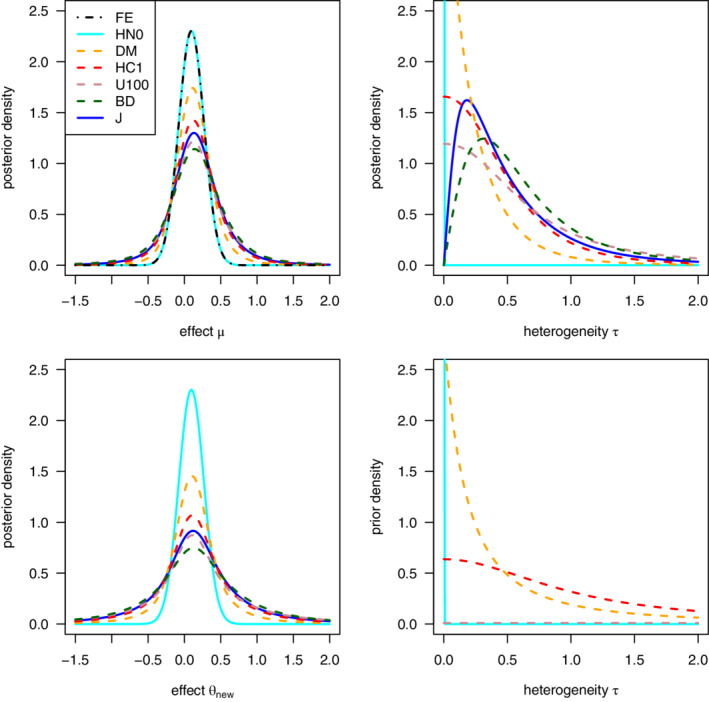
Auricular acupuncture data (k = 4), marginal posterior and heterogeneity prior densities: Top panels and bottom left panel: Marginal posterior for $\mu$, $\tau$ and the predicted effect ${\theta }_{\text{new}}$ based on the prior $\pi (\mu )\sim \mathrm{N}(0,4^2)$ and the heterogeneity priors listed in the legend in the top left panel. Bottom right panel: Density of the proper priors U100, DM, and HC1 in Table 1 and the proper HN0 benchmark prior (The improper priors are not shown here) [Colour figure can be viewed at wileyonlinelibrary.com]

FIGURE 2.

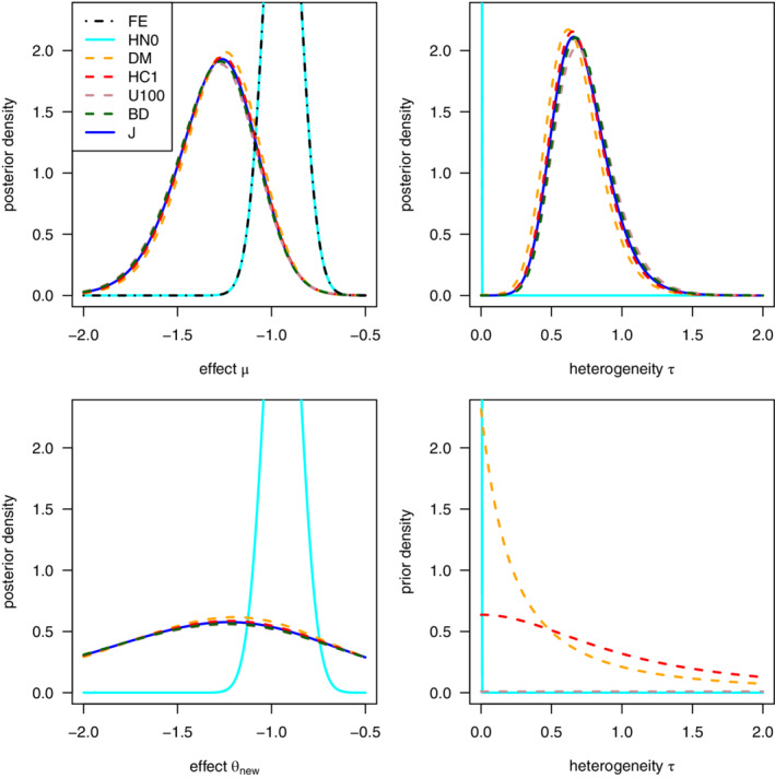
Respiratory tract infections data (k = 22), marginal posterior and heterogeneity prior densities: Top panels and bottom left panel: Marginal posterior for $\mu$, $\tau$ and the predicted effect ${\theta }_{\text{new}}$ based on the prior $\pi (\mu )\sim \mathrm{N}(0,4^2)$ and the heterogeneity priors listed in the legend in the top left panel. Bottom right panel: Density of the proper priors U100, DM, and HC1 in Table 1 and the proper HN0 benchmark prior (The improper priors are not shown here) [Colour figure can be viewed at wileyonlinelibrary.com]

In addition, we consider the improper (ie, its density does not integrate to any finite value) Berger‐Deely (BD in Table 1) heterogeneity prior, which has been introduced as an alternative to the improper uniform prior in the case where no or little prior information is available.²⁴ Note that the BD and the DM prior both depend on the data via the SD ${\sigma }_i$ values. If all SDs ${\sigma }_i$, i = 1, … , k, are equal, then the BD prior and Jeffreys reference prior J (see Table 2) are identical.²⁰ Although the BD prior is improper, the posterior distribution ${\text{po}}_{\text{BD}}(\psi )$ induced by BD is proper for all parameters $\psi \in \{\mu ,\tau ,{\theta }_1,\dots ,{\theta }_k,{\theta }_{\text{new}}\}$ if the dataset contains at least k = 2 studies.²⁰

3.3. Reference analysis

A reference prior is not necessarily a proper distribution, but rather it is frequently just a mathematical device (ie, a positive function) to be formally used in Bayes theorem to produce a reference posterior.¹¹ The posterior distribution based on a reference prior is maximally informed by the data and is called the reference posterior distribution. The reference posterior distribution functions as a benchmark, or a baseline, for the class of posterior distributions obtained from other admissible proper priors.⁹ According to Bernardo and Smith,⁶ the reference posterior should always be reported in a Bayesian analysis.

The original reference analysis⁶ proceeds according to the following four steps: First, given a Bayesian model and a dataset, a minimally informative reference prior is used to obtain a reference posterior. Second, an actual admissible prior of interest yields a corresponding posterior. Third, the posterior implied by the actual prior and the reference posterior are compared. Finally, this leads to indirect conclusions regarding the informativeness of the actual prior relative to the minimally informative reference prior.

By comparing different posterior distributions with the reference posterior benchmark, the relative impact of the underlying priors on the corresponding posterior results can be assessed.⁶ Bernardo and Smith⁶ recommended a reference analysis for the following two purposes: either as a “what if” baseline in considering a range of actual prior to posterior analyses, or as a default option, when there are insufficient resources for detailed elicitation of actual prior knowledge. A carefully conducted reference analysis may be very relevant in practice, because users are often not cognizant of the precise informativeness of the chosen priors.¹¹

Reference priors are a well‐accepted standard, useful in cases where it is difficult to elicit an appropriate subjective prior. However, they are not intended to replace subjective priors.¹⁰ Indeed, in cases that require a contribution of external information and some regularization by the prior, it is not necessarily ideal to add too little information to the data.¹, ⁵, ¹⁰ If an actual posterior has a small distance to the reference posterior, it only means that the actual heterogeneity prior adds only slightly more information to the data than the minimally informative reference prior. This distance does not reflect the quality or appropriateness of the actual subjective prior choice.

Recently, several publications have contributed important developments to the field of reference analysis, see, for example, Consonni et al.²⁵ The reference analysis has also become relevant in the context of the Bayesian meta‐analysis. As mentioned in Section 2, Bodnar et al¹⁵ used the methodology developed by Bodnar et al¹⁷ to compare the posterior descriptive statistics obtained from the reference posterior with results from the use of other priors and several classical meta‐analytical methods.

3.4. The reference prior and posterior benchmarks

The reference prior for the between‐study SD (Table 2) in the NNHM is implemented in the R package bayesmeta ²⁰ and can be accessed by specifying tau.prior=“Jeffreys”.¹⁵ For the reference analysis, we will consider this Jeffreys (J) reference prior.²⁰ Note that this prior is improper. However, the posterior benchmark distribution ${\text{po}}_{\mathrm{J}}(\psi )$ resulting from Jeffreys prior is proper in the Bayesian NNHM for all parameters $\psi \in \{\mu ,\tau ,{\theta }_1,\dots ,{\theta }_k,{\theta }_{\text{new}}\}$ if the dataset contains at least k = 2 studies.¹⁵, ¹⁷, ²⁰

In general, heterogeneity priors for $\tau$ can put their main probability mass on two sides of the minimally informative reference prior J: either on the side closer to $\tau =0$ (anticonservative) or on the side closer to $\tau =\infty$ (conservative). Whereas anticonservative heterogeneity priors cast doubt on the existence of random effects variation and allow the real between‐study SD $\tau$ to be underestimated, conservative priors can substantially overestimate the random effects variation.⁸ Note that this terminology follows the conventions in the meta‐analysis context,²⁰, ²⁶, ²⁷ whereas Gustafson et al⁸ use the term “conservative prior” differently in the context of general Bayesian hierarchical models. Posteriors induced by an anticonservative and a conservative heterogeneity prior could hypothetically end up equally far from the reference posterior benchmark J. To distinguish between these two kinds of priors, we take a familiar half‐normal prior HN($\lambda$) with a small scale parameter $\lambda$ as a benchmark (Table 2). A wide range of scale parameters $\lambda$ (from 1/600 to 1/100) were adequate and all computations ran smoothly. For computation, we fixed this scale parameter at a very small value, $\lambda =0.002$. We abbreviate the HN(0.002) prior as HN0 in the sequel. HN0 puts the majority of probability mass close to $\tau =0$ (mean =0.0016, SD = 0.0012, 2.5% quantile = 0.00006, median = 0.0013, 97.5% quantile = 0.0045) and is light‐tailed. Posteriors induced by HN0 lead to benchmark posterior distributions ${\text{po}}_{\text{HN0}}(\psi )$ for all parameters $\psi \in \{\mu ,\tau ,{\theta }_1,\dots ,{\theta }_k,{\theta }_{\text{new}}\}$ in the Bayesian NNHM.

We consider one additional posterior benchmark po_FE which applies only to the overall mean parameter $\mu$. It corresponds to assuming a point mass at $\tau =0$, which leads to the normal benchmark FE posterior provided in Equation (2).

3.5. The Hellinger distance and its normal calibration

The Hellinger distance²⁸ is conveniently defined in two steps. First, for two probability densities ${\pi }_0$ and ${\pi }_1$, the Bhattacharyya coefficient (BC) is defined as

$$\text{BC}({\pi }_1,{\pi }_0)={\int }_{-\infty }^{\infty }\sqrt{{\pi }_1(x){\pi }_0(x)}dx.$$

The BC quantifies the affinity of the two densities. BC attains the maximal value 1 if the two densities are equal and the minimal value 0 if the supports of the densities do not overlap. The Hellinger distance between the two densities is then given by

$$\mathrm{H}({\pi }_1,{\pi }_0)=\sqrt{\frac{1}{2}{\int }_{-\infty }^{\infty }{\left(\sqrt{{\pi }_1(x)}-\sqrt{{\pi }_0(x)}\right)}^{2}dx}=\sqrt{1-\text{BC}({\pi }_1,{\pi }_0)}.$$

The Hellinger distance is symmetric (ie, $\mathrm{H}({\pi }_1,{\pi }_0)=\mathrm{H}({\pi }_0,{\pi }_1)$) and attains the value 1 for complete disagreement and the value 0 for complete agreement of the two densities. We will use the Hellinger distance H to compare the marginal posterior of interest ${\text{po}}_{\text{act}}(\psi )$ with the reference posterior ${\text{po}}_{\mathrm{J}}(\psi )$ and the posterior benchmark ${\text{po}}_{\text{HN0}}(\psi )$, for $\psi \in \{\mu ,\tau ,{\theta }_1,\dots ,{\theta }_k,{\theta }_{\text{new}}\}$. In the case studies, the actual heterogeneity priors of interest (act) are DM, HC1, U100, and BD.

To interpret Hellinger distance values, Roos et al²⁹ proposed a calibration of the Hellinger distance, which is based on two unit variance normal distributions with shifted locations. The choice of normal distributions for the calibration is convenient because the normal distribution is well known. Moreover, any density can be approximated to the first order by a normal distribution.³⁰, ³¹ Roos et al²⁹ showed that for a given Hellinger distance value h, we have

$$\mathrm{H}(\mathrm{N}(\mu (h),1),\mathrm{N}(0,1))=h,\text{where}\mu (h)=\sqrt{-8\log (1-h^2)}.$$ (3)

We extend this calibration and provide estimates of the area of the overlap (AO) of the two shifted normal distributions:

$$\text{AO}(\mu (h))=\mathrm{\Phi }(\mu (h)/2;\mu (h),1)+(1-\mathrm{\Phi }(\mu (h)/2;0,1)),$$ (4)

where $\mathrm{\Phi }(·)$ denotes the normal cumulative distribution function. Table 3 shows the normal calibration of the Hellinger distance with the shift $\mu (h)$ and the area of overlap $\text{AO}(\mu (h))$ for a selection of Hellinger distance values h. The function $\mu (h)$ is almost linear for small values of h, more precisely $\mu (h)\approx 2.83h$ for h < 0.5. Note that the Hellinger distance h = 0.451, which corresponds to the shift $\mu =1.349$ and the area of overlap $\text{AO}(\mu (h))=0.5$, is a convenient point of reference. Two densities with h < 0.451 have AO > 0.5 and vice versa. An application of this calibration is given in Section 4.3.

TABLE 3.

Normal calibration of the Hellinger distance h in terms of the shift $\mu (h)$ between two unit variance normal distributions and their area of overlap $\text{AO}(\mu (h))$ defined in Equations (3) and (4)

h	$\mu (h)$	$\text{AO}(\mu (h))$	h	$\mu (h)$	$\text{AO}(\mu (h))$	h	$\mu (h)$	$\text{AO}(\mu (h))$
0.010	0.028	0.989	0.100	0.284	0.887	0.910	3.753	0.061
0.020	0.057	0.977	0.200	0.571	0.775	0.920	3.871	0.053
0.030	0.085	0.966	0.300	0.869	0.664	0.930	4.002	0.045
0.040	0.113	0.955	0.400	1.181	0.555	0.940	4.148	0.038
0.050	0.142	0.944	0.500	1.517	0.448	0.950	4.315	0.031
0.060	0.170	0.932	0.600	1.890	0.345	0.960	4.513	0.024
0.070	0.198	0.921	0.700	2.321	0.246	0.970	4.757	0.017
0.080	0.227	0.910	0.800	2.859	0.153	0.980	5.082	0.011
0.090	0.255	0.899	0.900	3.645	0.068	0.990	5.598	0.005

Abbreviation: AO, area of the overlap of two shifted normal distributions.

3.6. Posterior reference analysis

The post‐RA in the Bayesian NNHM quantifies the informativeness of any chosen actual heterogeneity prior in relation to the minimally informative, improper reference prior indirectly based on proper marginal posteriors. For the post‐RA, we suggest two posterior benchmarks ${\text{po}}_{\text{HN0}}(\psi )$ and ${\text{po}}_{\mathrm{J}}(\psi )$, where ${\text{po}}_{\mathrm{J}}(\psi )$ denotes the marginal posterior distribution for $\psi$ under Jeffreys reference prior J for $\tau$ (Table 2), for $\psi \in \{\mu ,\tau ,{\theta }_1,\dots ,{\theta }_k,{\theta }_{\text{new}}\}$. The actual prior of interest pri_act leads to marginal posteriors ${\text{po}}_{\text{act}}(\psi )$ for all parameters $\psi \in \{\mu ,\tau ,{\theta }_1,\dots ,{\theta }_k,{\theta }_{\text{new}}\}$ in the Bayesian random effects model. Comparison of ${\text{po}}_{\text{act}}(\psi )$ with the benchmarks ${\text{po}}_{\text{HN0}}(\psi )$ and ${\text{po}}_{\mathrm{J}}(\psi )$ by means of the Hellinger distance leads to $\mathrm{H}({\text{po}}_{\text{HN0}}(\psi ),{\text{po}}_{\text{act}}(\psi ))$ and $\mathrm{H}({\text{po}}_{\text{act}}(\psi ),{\text{po}}_{\mathrm{J}}(\psi ))$ estimates for each parameter $\psi$. These estimates introduce an indirect partial ordering of the informativeness of priors for the Bayesian NNHM based on the marginal posteriors, because they specify if pri_act leads to posterior results ${\text{po}}_{\text{act}}(\psi )$ which are closer to ${\text{po}}_{\text{HN0}}(\psi )$ or ${\text{po}}_{\mathrm{J}}(\psi )$ for each parameter $\psi$. The induced partial ordering of priors is always with respect to a certain parameter $\psi$. This means that one may get a different ordering for $\mu$ than for $\tau$. For the parameter $\mu$, we additionally consider the FE benchmark FE and proceed with the corresponding marginal posterior for $\mu$ in the same way as for the J and HN0 benchmarks.

With the two HN0 and J benchmarks, we can decide whether the actual prior is anticonservative or conservative for the parameter of interest $\psi$. If the Hellinger distance between the actual posterior and the po_HN0 benchmark is smaller than the Hellinger distance between the po_HN0 benchmark and the reference posterior po_J, that is, $\mathrm{H}({\text{po}}_{\text{HN0}}(\psi ),{\text{po}}_{\text{act}}(\psi ))<\mathrm{H}({\text{po}}_{\text{HN0}}(\psi ),{\text{po}}_{\mathrm{J}}(\psi ))$, then the actual heterogeneity prior is anticonservative (puts more probability mass on small $\tau$ values than the reference prior). If we have $\mathrm{H}({\text{po}}_{\text{HN0}}(\psi ),{\text{po}}_{\text{act}}(\psi ))>\mathrm{H}({\text{po}}_{\text{HN0}}(\psi ),{\text{po}}_{\mathrm{J}}(\psi ))$, then the actual heterogeneity prior is conservative (puts more probability mass on large $\tau$ values than the reference prior).

In order to distinguish anticonservative and conservative heterogeneity priors with respect to the reference prior, we define a signed informativeness. The informativeness of an actual heterogeneity prior H(po_act, po_J) is multiplied by the sign of the difference H(po_HN0, po_act) ‐ H(po_HN0, po_J). The sign of this difference is negative when the po_act is closer to po_HN0 than po_J, indicating that the actual heterogeneity prior is anticonservative relative to the reference heterogeneity prior J. By contrast, the sign of this difference is positive for po_act that are further away from po_HN0 than po_J, indicating that the actual heterogeneity prior is conservative relative to the reference heterogeneity prior J.

3.7. Platykurtic and leptokurtic distributions

Now we introduce the definition of a platykurtic and leptokurtic posterior distribution ${\text{po}}_{\text{act}}(\psi )$ induced by an actual heterogeneity prior relative to the reference posterior ${\text{po}}_{\mathrm{J}}(\psi )$ for $\psi \in \{\mu ,{\theta }_{\text{new}}\}$. If the marginal posterior po_act has lighter (thinner) tails than the marginal posterior po_J, then the posterior po_act is platykurtic with respect to po_J. Platykurtic posterior distributions have a smaller spread than po_J and their posterior densities are more peaky than po_J. If a po_act has heavier (fatter) tails than po_J, we call it leptokurtic with respect to po_J. The spread of a leptokurtic po_act is larger than the spread of po_J, and the marginal posterior density of po_act is flatter than po_J. This definition follows the definition of platykurtic and leptokurtic distributions relative to a normal distribution with the normal distribution replaced by the reference posterior po_J.³²

Whether a posterior distribution is platykurtic or leptokurtic can have direct practical implications. If a posterior distribution is platykurtic, then the 95% CrI for the overall mean parameter $\mu$ is shorter. Consequently, 0 may be excluded from that CrI, thus producing a rather optimistic inference. By contrast, a leptokurtic distribution has a longer 95% CrI. In this case, 0 may be contained in the 95% CrI for the overall mean parameter $\mu$, thus producing a cautious inference.

3.8. R package ra4bayesmeta

The functions to perform the post‐RA are bundled in the R package ra4bayesmeta (https://cran.r‐project.org/package=ra4bayesmeta), entitled “Reference Analysis for Bayesian Meta‐Analysis.” The main function post_RA produces a table with posterior summaries and Hellinger distance estimates, see Table 4 in Section 4.1 for an example. Alternative benchmarks can be studied using the more flexible function post_RA_fits. This package also contains a function for the normal calibration of Hellinger distances and a function to produce density plots as shown in Figure 1, as well as the datasets used in the case studies. The functions operate on data frames compatible with the bayesmeta package.

TABLE 4.

AA data (k = 4), post‐RA: For each parameter $\psi \in \{\mu ,\tau ,{\theta }_{\text{new}}\}$ and each actual heterogeneity prior pri_act specified in the second column, the following estimates for the marginal posterior ${\text{po}}_{\text{act}}(\psi )$ are given: The posterior median, the equi‐tailed 95% CrI, the length L(CrI) of that CrI, the Hellinger distance to the po_HN0 benchmark and the signed informativeness (Sign. Inf.) sign(H(po_HN0, po_act) − H(po_HN0, po_J))H(po_act, po_J)

Par.	priact	Median (95% CrI)	L(CrI)	H(poHN0, poact)	Sign. Inf.
$\mu$	FE	0.10 (−0.24, 0.44)	0.68	0.000	−0.326
	HN0	0.10 (−0.24, 0.44)	0.68	0.000	−0.326
	DM	0.12 (−0.40, 0.74)	1.13	0.196	−0.136
	HC1	0.14 (−0.58, 0.96)	1.54	0.291	−0.041
	U100	0.15 (−0.98, 1.35)	2.33	0.366	+0.064
	BD	0.16 (−0.80, 1.19)	1.99	0.373	+0.049
	J	0.15 (−0.68, 1.07)	1.75	0.326	0.000
$\tau$	HN0	0.00 ( 0.00, 0.00)	0.00	0.000	−0.994
	DM	0.16 ( 0.01, 1.05)	1.05	0.922	−0.324
	HC1	0.33 ( 0.02, 1.55)	1.53	0.953	−0.132
	U100	0.48 ( 0.02, 3.28)	3.26	0.961	−0.147
	BD	0.52 ( 0.08, 2.24)	2.16	0.996	+0.118
	J	0.39 ( 0.05, 1.98)	1.92	0.994	0.000
${\theta }_{\text{new}}$	HN0	0.10 (−0.24, 0.44)	0.68	0.000	−0.461
	DM	0.12 (−0.78, 1.14)	1.92	0.300	−0.173
	HC1	0.13 (−1.28, 1.67)	2.96	0.418	−0.050
	U100	0.14 (−2.33, 2.71)	5.04	0.492	+0.072
	BD	0.16 (−1.86, 2.24)	4.10	0.516	+0.063
	J	0.14 (−1.56, 1.95)	3.51	0.461	0.000

Note: FE for $\mu$ denotes the fixed effects model, which corresponds to a point mass at $\tau =0$ as heterogeneity prior. Note that posterior estimates of $\mu$ induced by FE and the highly anticonservative HN0 prior match very well.

Abbreviations: AA, auricular acupuncture; BD, Berger‐Deely; DM, DuMouchel; post‐RA, posterior reference analysis.

4. RESULTS

This section reports the post‐RA of the AA (k = 4) and RTI (k = 22) data. Moreover, it compares some results obtained for these two datasets.

4.1. Post‐RA for the AA dataset

Table 4 provides posterior medians, equi‐tailed 95% CrIs, their lengths L(CrI), and post‐RA of $\mu$, $\tau$, and ${\theta }_{\text{new}}$ for AA obtained for DM, HC1, U100, and BD heterogeneity priors. Posterior medians and equi‐tailed 95% CrIs are also illustrated in a forest plot in the left column of Figure 3. Moreover, the relation between the signed informativeness of heterogeneity priors and L(CrI) is depicted in Figure 4. The posterior estimates and informativeness values for the random effect parameters ${\theta }_1$, …, ${\theta }_4$ are provided in Table 4 of the Supplementary Material.

FIGURE 3.

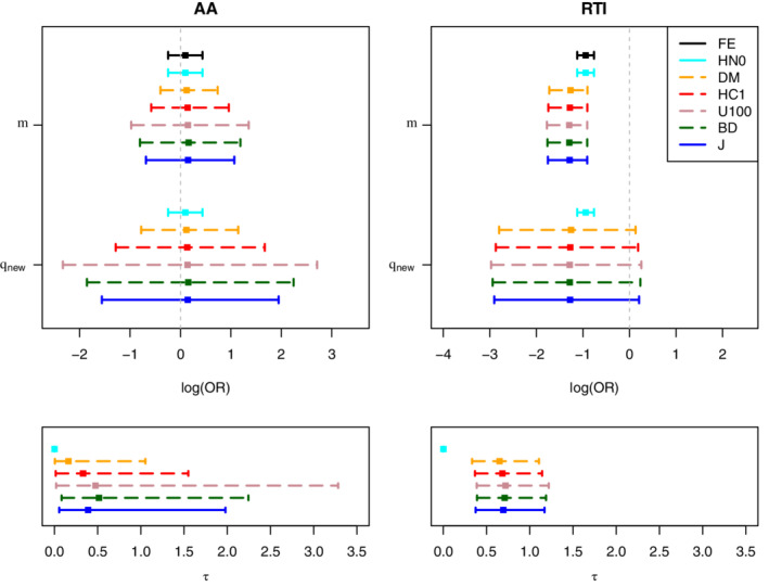
Auricular acupuncture (AA) data (k = 4, left column) and respiratory tract infections (RTI) data (k = 22, right column), forest plots with posterior estimates for the parameters $\mu$, ${\theta }_{\text{new}}$, and $\tau$: The posterior median (square) and equi‐tailed 95% credible interval is shown for each heterogeneity prior listed in the legend [Colour figure can be viewed at wileyonlinelibrary.com]

FIGURE 4.

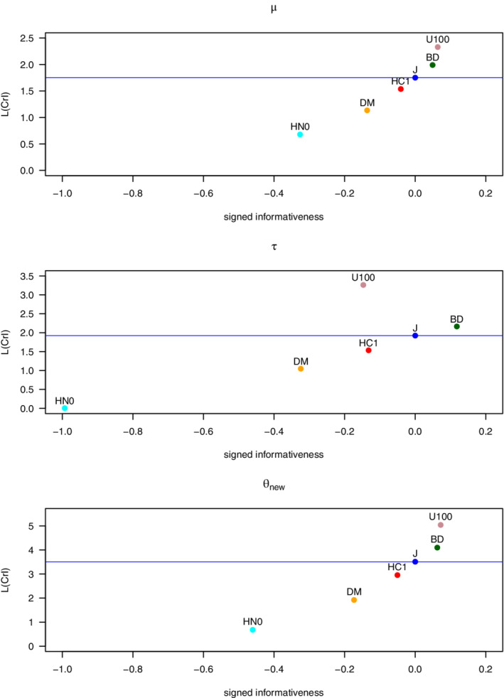
Auricular acupuncture data (k = 4), estimates from Table 4: The relation between the signed informativeness of heterogeneity priors sign(H(po_HN0, po_act) − H(po_HN0, po_J))×H(po_act, po_J) and the corresponding length L(CrI) of the 95% credible interval for the parameters $\mu$, $\tau$, and ${\theta }_{\text{new}}$. The horizontal blue lines indicate L(CrI) induced by the reference prior J. For $\mu$ and ${\theta }_{\text{new}}$, L(CrI) increases with increasing signed informativeness [Colour figure can be viewed at wileyonlinelibrary.com]

Inspection of the H(po_act, po_J) estimates for $\mu$, that is, the absolute values of the numbers in the last column of Table 4, reveals that HC1 is the least informative heterogeneity prior for $\mu$, because it induces a posterior po_HC1 that attains the smallest distance (H = 0.041) to the reference posterior po_J. Note that po_HC1 is even closer to the reference posterior than the posterior induced by the improper BD heterogeneity prior (H = 0.049). By contrast, DM is the most informative heterogeneity prior for $\mu$, because it is farthest from the reference posterior po_J and attains H = 0.136. The resulting post‐RA ranking of informativeness from smallest to largest is HC1, BD, U100, DM.

Inspection of the H(po_HN0, po_act) column of Table 4 for $\mu$ reveals that DM (H = 0.196) and HC1 (H = 0.291) lead to posteriors that are closer to po_HN0 than po_J (H = 0.326). This means that DM and HC1 are on the anticonservative side of the reference prior J. By contrast, po_BD (H = 0.373) and po_U100 (H = 0.366) are more distant from po_HN0 than po_J (H = 0.326). This means that BD and U100 are on the conservative side of the reference prior J.

Figure 3 (left column) shows po_act and po_J posterior medians and 95% CrIs for $\mu$ and demonstrates whether po_act is platykurtic or leptokurtic with respect to po_J. Recall that anticonservative heterogeneity priors put more mass on heterogeneity values that are smaller than those governed by J, so they are more informative for $\tau =0$ than J. We found that these priors produce platykurtic po_act with respect to po_J for $\mu$. On the other hand, conservative heterogeneity priors put more mass on heterogeneity values that are larger than those governed by J and thus are more informative for $\tau =\infty$ than J. These produce leptokurtic po_act with respect to po_J for $\mu$.

There is a strong link between the platykurtic and leptokurtic status of po_act, the length of CrI, and the signed informativeness values for $\mu$ in Figure 4. As Figure 3 (left column) and Figure 4 show, the anticonservative DM and HC1 priors (which have negative signed informativeness) lead to CrI($\mu$) that are shorter than CrI($\mu$) of the reference posterior. These two priors induce platykurtic posteriors relative to the reference posterior, see Figure 1 (top left panel). By contrast, the conservative BD and U100 (which have positive signed informativeness) lead to CrI($\mu$) that are longer than CrI($\mu$) of the reference posterior. These two priors induce leptokurtic posteriors.

Note that the sign and the value of informativeness of the heterogeneity prior depends on the parameter under consideration. For example, for $\tau$, BD is the least informative (H = 0.118 in the last column of Table 4) and the only conservative heterogeneity prior (more distant from po_HN0 than po_J with H = 0.996 > 0.994). By contrast, for ${\theta }_{\text{new}}$, the order of informativeness of DM, HC1, U100, and BD is the same as for $\mu$.

4.2. Post‐RA for the RTI dataset

The results of the post‐RA for the RTI dataset are summarized in Table 5. In general, the qualitative findings for the RTI dataset with k = 22 are similar to the ones for the smaller AA dataset (k = 4) in the previous section. For all the parameters $\mu ,\tau$ and ${\theta }_{\text{new}}$, the post‐RA ranking based on the distance H(po_act, po_J) is the same, from smallest to largest: HC1, BD, U100, DM. This is the same ranking as for the parameters $\mu$ and ${\theta }_{\text{new}}$ and the AA dataset.

TABLE 5.

RTI data (k = 22), post‐RA: For each parameter $\psi \in \{\mu ,\tau ,{\theta }_{\text{new}}\}$ and each actual heterogeneity prior pri_act specified in the second column, the following estimates for the marginal posterior ${\text{po}}_{\text{act}}(\psi )$ are given: The posterior median, the equi‐tailed 95% CrI, the length L(CrI) of that CrI, the Hellinger distance to the po_HN0 benchmark and the signed informativeness (Sign. Inf.) sign(H(po_HN0, po_act) − H(po_HN0, po_J))H(po_act, po_J)

Par.	priact	Median (95% CrI)	L(CrI)	H(poHN0, poact)	Sign. Inf.
$\mu$	FE	−0.94 (−1.12, −0.76)	0.36	0.000	−0.729
	HN0	−0.94 (−1.12, −0.76)	0.36	0.000	−0.729
	DM	−1.27 (−1.72, −0.90)	0.82	0.714	−0.032
	HC1	−1.28 (−1.74, −0.91)	0.84	0.726	−0.008
	U100	−1.29 (−1.77, −0.91)	0.87	0.735	+0.017
	BD	−1.29 (−1.76, −0.91)	0.85	0.734	+0.011
	J	−1.29 (−1.75, −0.91)	0.85	0.729	0.000
$\tau$	HN0	0.00 ( 0.00, 0.00)	0.00	0.000	−1.000
	DM	0.65 ( 0.33, 1.11)	0.77	0.997	−0.083
	HC1	0.68 ( 0.37, 1.14)	0.78	0.999	−0.023
	U100	0.72 ( 0.39, 1.22)	0.83	0.999	−0.046
	BD	0.71 ( 0.39, 1.19)	0.80	1.000	+0.030
	J	0.69 ( 0.37, 1.17)	0.80	1.000	0.000
${\theta }_{\text{new}}$	HN0	−0.94 (−1.12, −0.76)	0.36	0.000	−0.719
	DM	−1.26 (−2.80, 0.13)	2.93	0.707	−0.028
	HC1	−1.27 (−2.87, 0.18)	3.06	0.716	−0.008
	U100	−1.28 (−2.97, 0.25)	3.23	0.724	+0.016
	BD	−1.28 (−2.94, 0.23)	3.17	0.723	+0.009
	J	−1.28 (−2.91, 0.21)	3.11	0.719	0.000

Note: FE for $\mu$ denotes the fixed effects model, which corresponds to a point mass at $\tau =0$ as heterogeneity prior. Note that posterior estimates of $\mu$ induced by FE and the highly anticonservative HN0 prior match very well.

Abbreviations: BD, Berger‐Deely; DM, DuMouchel, RTI, respiratory tract infections.

The posterior densities for $\mu$ and ${\theta }_{\text{new}}$ shown in Figure 2 and the CrIs in Figure 3 are very close to the reference posterior for all four actual heterogeneity priors considered, making it difficult to detect platykurtic and leptokurtic posteriors based on these figures. Comparing the length of the 95% CrIs for $\mu$ in Table 5 reveals that the DM and HC1 priors have shorter CrIs than the reference posterior and are thus platykurtic with respect to the reference posterior. As for the AA dataset, these two priors are anticonservative relative to the reference prior J.

By contrast, the U100 and BD priors induce posteriors for $\mu$ that have longer CrIs than the reference posterior and are thus leptokurtic with respect to the reference posterior. The U100 and BD priors induce marginal posteriors for $\mu$ which are farther away from the po_HN0 benchmark than the reference posterior po_J (see the signed informativeness estimates in the last column of Table 5) and are thus conservative relative to the reference prior J.

4.3. Comparison of the results for the AA data (k  =  4) and the RTI data (k  =  22)

For the RTI dataset, setting $\tau =0$ (FE model) is a very strong assumption. As illustrated in the top right panel in Figure 3, this assumption leads to posterior inference that strongly differs from the inference based on the minimally informative reference prior (J) and from that based on the DM, HC1, U100, and BD heterogeneity priors. The discrepancy between the posterior ${\text{po}}_{\text{HN0}}(\mu )$ and other marginal posteriors for $\mu$ (except the FE benchmark) demonstrates how neglecting heterogeneity (by assuming $\tau =0$) impacts posterior inference, which leads to an estimated overall log odds ratio closer to 0 for RTI. Note that for AA, setting $\tau =0$ leads to comparable results to those for the DM, HC1, U100, and BD heterogeneity priors.

Comparison of the H(po_act, po_J) estimates for the post‐RA in Figure 5 (top, see also Tables 4 and 5) for the AA and RTI data reveals that these Hellinger distances between the marginal posteriors for $\mu$, ${\theta }_{\text{new}}$ and $\tau$ are much smaller for RTI (k = 22) than for AA (k = 4). Consequently, the DM, HC1, U100, and BD priors are more informative for the small AA dataset with k = 4 studies than for the larger RTI dataset with k = 22 studies. This appears to be a consequence of the smaller sample size, that is, the number of studies included in the meta‐analysis, in the AA dataset.

FIGURE 5.

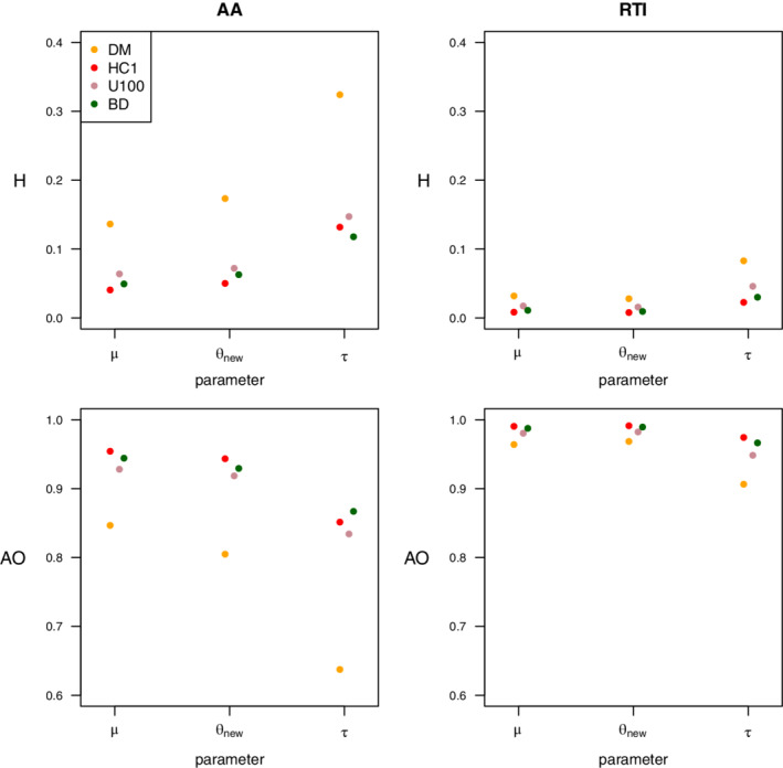
Auricular acupuncture (AA) data (k = 4, left column) and respiratory tract infections (RTI) data (k = 22, right column), absolute values of signed informativeness estimates from the post‐RA: Top row: For the parameter $\psi \in \{\mu ,{\theta }_{\text{new}},\tau \}$ indicated on the x‐axis, the dots show the Hellinger distances $\mathrm{H}({\text{po}}_{\text{act}}(\psi ),{\text{po}}_{\mathrm{J}}(\psi ))$ between the marginal Jeffreys reference posterior and the marginal posterior induced by the actual heterogeneity prior pri_act, act ∈ {DM, HC1, U100, BD}. The bottom row displays the areas of overlap corresponding to the Hellinger distances shown in the top row [Colour figure can be viewed at wileyonlinelibrary.com]

Figure 5 (bottom) applies the normal calibration of the Hellinger distance introduced in Section 3.5. This calibration demonstrates that the area of overlap of po_act and the reference posterior po_J is larger for RTI than for AA. According to Equations (3) and (4) (see also Table 3), the informativeness estimate H = 0.136 for $\mu$ induced by the most informative DM heterogeneity prior applied to AA corresponds to a shift of 0.387 between two unit variance normal distributions and an associated area of overlap of 0.847. The informativeness estimate H = 0.041 of the least informative HC1 applied to AA corresponds to a shift of 0.115 between two unit variance normal distributions, which have an area of overlap equal to 0.954. By contrast, the corresponding numbers for DM and HC1 applied to RTI indicate that the posteriors of actual heterogeneity priors better match the reference posterior. Indeed, H = 0.032 for DM corresponds to a shift of 0.090 and an associated area of overlap of 0.964 and H = 0.008 for HC1 corresponds to a shift of 0.024 between two unit variance normal distributions and an associated area of overlap of 0.991.

In conclusion, we found that the informativeness depends on the number of studies, the heterogeneity prior, and the parameter under consideration. Although U100 is conservative for $\mu$ and ${\theta }_{\text{new}}$ for both AA and RTI, it is anticonservative for $\tau$. U100 assigns probability mass to values of $\tau$ only in the interval [0, 100]. This truncation may cause the switch in conservativeness between parameters.

5. DISCUSSION

The post‐RA is a diagnostic tool that creates a partial ordering of the informativeness of heterogeneity priors with respect to the minimally informative reference prior. We applied the post‐RA to three proper (DM, HC1, U100) and one improper BD heterogeneity priors of interest across two medical case studies (AA, RTI) and demonstrated that post‐RA is applicable to any heterogeneity prior, provided that the resulting posterior is proper.

The distances between the posteriors of interest and the reference posterior quantify the heterogeneity prior informativeness with respect to the reference prior J benchmark. However, we found that two posteriors induced by an anticonservative and a conservative heterogeneity prior can have equal distances to the reference posterior. To resolve this ambiguity, we considered one additional highly anticonservative benchmark HN0, which concentrated the majority probability mass on heterogeneity values close to 0. HN0 produced posteriors for the overall mean parameter that matched well with the posterior of the FE model, which assumes $\tau =0$. Moreover, HN0 indicated whether heterogeneity priors of interest were anticonservative or conservative with respect to the reference benchmark J.

Based on the information gained from these (HN0, J) benchmarks, we were able to determine that anticonservative heterogeneity priors for the overall mean lead to platykurtic posteriors, shorter 95% CrI, and optimistic inference. The shortest 95% CrI was attained by DM, which was the most informative anticonservative heterogeneity prior. By contrast, conservative heterogeneity priors for the overall mean lead to leptokurtic posteriors, longer 95% CrI, and cautious inference. The longest 95% CrI was attained by U100, which was the most informative conservative heterogeneity prior considered. Thus, U100 was conservative and more informative than BD for the overall mean of both AA and RTI. These results complemented the analysis provided by Bodnar et al.¹⁵

Note that the Supplementary Material describes alternative benchmark distributions. In fact, there we use proper distributions that generalize the improper BD prior and cover the conventional prior as a special case.²⁴ Similar distributions have already been used to define anticonservative heterogeneity priors for Bayesian hierarchical models.⁸ In the Supplementary Material, three benchmark distributions are considered in order to discriminate between strongly anticonservative, reference affine, and strongly conservative heterogeneity priors. For AA and RTI, these three benchmarks showed that although U100 is conservative for the overall mean, it is still reference affine as compared with the highly conservative benchmark. Moreover, we proposed a prior reference analysis (pri‐RA) based on a reverse Bayes approach and demonstrated that the post‐RA was more successful than the pri‐RA in ranking the informativeness of heterogeneity priors.

The comparison of the results provided by post‐RA based on the two benchmarks in the main text (HN0, J) and on the three benchmarks of the Supplementary Material showed that findings remain stable when a different distribution is assigned to the highly anticonservative benchmark. This indicates that the specific choice of the benchmark distribution is not critical to establishing the order of informativeness. We only need a reasonable suggestion for benchmarks to let an ordering emerge,³³ and if necessary, alternative benchmark distributions can be easily incorporated into our principled approach. Thus, we chose to focus on the two HN0 and J benchmarks, because these benchmarks are easy to understand and provide answers to most of the questions asked in applications.

In this article, we used bayesmeta to estimate Bayesian NNHMs. This approach relies on using an accurate Bayesian numerical approximation of the full Bayesian NNHM.²⁰, ³⁴ This numerical approximation facilitates fast estimation of Bayesian NNHMs and dispenses with convergence diagnostics, which are necessary for MCMC sampling approaches. Moreover, bayesmeta provides a wide range of priors and is, therefore, a convenient software to use for post‐RA.

For Bayesian NNHMs, we observed excellent agreement between the results obtained from bayesmeta and the corresponding results from JAGS, Stan, and R‐INLA. Consequently, our findings provided by post‐RA are not specific to bayesmeta, but valid more generally. In the future, however, we plan to make the post‐RA methodology for the Bayesian NNHM accessible to the R‐INLA environment and to general‐purpose MCMC engines for Bayesian estimation such as JAGS, Stan, OpenBUGS, and BayesX.

Currently, our principled post‐RA methodology has been implemented as an add‐on functionality for the bayesmeta environment and the R code is freely accessible in the R package ra4bayesmeta on CRAN (https://cran.r‐project.org/package=ra4bayesmeta). Thus, post‐RA can be used directly by practitioners familiar with the bayesmeta environment in a number of different fields, and in particular in medical applications.

Overall, the importance of assessing the informativeness of heterogeneity priors depends on the data. We found that in data‐dominated cases, when the posterior is dominated by a peaked likelihood function (RTI, k = 22), results are similar regardless of which actual heterogeneity prior is used.¹⁰ However, in situations where the impact of data is small (AA, k = 4) and the Bayesian meta‐analysis may lead to posteriors that are dominated by prior assumptions, it is important to carefully assess the informativeness of heterogeneity priors. Post‐RA determines how informative a heterogeneity prior is for the actual data as compared with the minimally informative reference prior. Hence, it can help in practice by providing a principled assessment of “vagueness” and “weak informativeness,” thus supporting a better understanding of the validity of posterior inference in evidence‐based medicine and many other research fields.

CONFLICT OF INTEREST

The authors declare no potential conflict of interests.

Supporting information

Appendix S1

Ott M, Plummer M, Roos M. How vague is vague? How informative is informative? Reference analysis for Bayesian meta‐analysis. Statistics in Medicine. 2021;40:4505–4521. 10.1002/sim.9076

DATA AVAILABILITY STATEMENT

The data for the three case studies in the main text and the Supplementary Material are provided in Tables 3, 12, and 21 in the Supplementary Material. The AA and RTI data are also available in the published paper by Bodnar et al (15, tables I and II). The three datasets are included in the R package ra4bayesmeta (https://cran.r‐project.org/package=ra4bayesmeta) under the names aa, rti, and aom. This freely accessible R package implements the methodology for the reference analysis proposed in this article.

REFERENCES

- 1.Spiegelhalter DJ, Abrams KR, Myles JP. Bayesian Approaches to Clinical Trials and Health‐Care Evaluation. Chichester, England: John Wiley & Sons; 2004. [Google Scholar]
- 2.Friede T, Röver C, Wandel S, Neuenschwander B. Meta‐analysis of two studies in the presence of heterogeneity with applications in rare diseases. Biom J. 2017;59(4):658‐671. 10.1002/bimj.201500236. [DOI] [PMC free article] [PubMed] [Google Scholar]
- 3.Lesaffre E, Lawson AB. Bayesian Biostatistics. Chichester, England: John Wiley & Sons; 2012. [Google Scholar]
- 4.Lunn D, Jackson C, Best N, Thomas A, Spiegelhalter D. The BUGS Book: A Practical Introduction to Bayesian Analysis. Chapman & Hall/CRC Press: Boca Raton, FL; 2013. [Google Scholar]
- 5.Gelman A, Carlin JB, Stern HS, Dunson DB, Vehtari A, Rubin DB. Bayesian Data Analysis. 3rd ed.Boca Raton, FL: Chapman & Hall/CRC Press; 2014. [Google Scholar]
- 6.Bernardo JM, Smith AFM. Bayesian Theory. Chichester, England: John Wiley & Sons; 2000. [Google Scholar]
- 7.Box GEP, Tiao GC. Bayesian Inference in Statistical Analysis. Reading, MA: Addison–Wesley; 1973. [Google Scholar]
- 8.Gustafson P, Hossain S, MacNab YC. Conservative prior distributions for variance parameters in hierarchical models. Can J Stat. 2006;34(3):377‐390. 10.1002/cjs.5550340302. [DOI] [Google Scholar]
- 9.Bernardo JM. Reference posterior distributions for Bayesian inference. J R Stat Soc Ser B Stat Methodol. 1979;41(2):113‐147. [Google Scholar]
- 10.Kass RE, Wasserman L. The selection of prior distributions by formal rules (Corr 1998V93 p. 412). J Am Stat Assoc. 1996;91(435):1343‐1370. 10.2307/2291752. [DOI] [Google Scholar]
- 11.Irony TZ, Singpurwalla ND. Non‐informative priors do not exist A dialogue with José M. Bernardo. J Stat Plan Infer. 1997;65(1):159‐177. 10.1016/S0378-3758(97)00074-8. [DOI] [Google Scholar]
- 12.Berger JO, Bernardo JM, Sun D. The formal definition of reference priors. Ann Stat. 2009;37(2):905‐938. 10.1214/07-AOS587. [DOI] [Google Scholar]
- 13.Gelman A, Hennig C. Beyond subjective and objective in statistics. J R Stat Soc Ser A Stat Soc. 2017;180(4):967‐1033. 10.1111/rssa.12276. [DOI] [Google Scholar]
- 14.Lambert PC, Sutton AJ, Burton PR, Abrams KR, Jones DR. How vague is vague? a simulation study of the impact of the use of vague prior distributions in MCMC using WinBUGS. Stat Med. 2005;24(15):2401‐2428. 10.1002/sim.2112. [DOI] [PubMed] [Google Scholar]
- 15.Bodnar O, Link A, Arendacká B, Possolo A, Elster C. Bayesian estimation in random effects meta‐analysis using a non‐informative prior. Stat Med. 2017;36(2):378‐399. 10.1002/sim.7156. [DOI] [PubMed] [Google Scholar]
- 16.Gelman A. Prior distributions for variance parameters in hierarchical models (comment on article by Browne and Draper). Bayesian Anal. 2006;1(3):515‐534. 10.1214/06-BA117A. [DOI] [Google Scholar]
- 17.Bodnar O, Link A, Elster C. Objective Bayesian inference for a generalized marginal random effects model. Bayesian Anal. 2016;11(1):25‐45. 10.1214/14-BA933. [DOI] [Google Scholar]
- 18.Bernardo JM. The concept of exchangeability and its applications. Far East J Math Sci. 1996;4:111‐121. [Google Scholar]
- 19.Sutton AJ, Abrams KR. Bayesian methods in meta‐analysis and evidence synthesis. Stat Methods Med Res. 2001;10(4):277‐303. 10.1177/096228020101000404. [DOI] [PubMed] [Google Scholar]
- 20.Röver C. Bayesian random‐effects meta‐analysis using the bayesmeta R package. J Stat Softw. 2020;93(6):1‐51. 10.18637/jss.v093.i06. [DOI] [Google Scholar]
- 21.Bender R, Friede T, Koch A, et al. Methods for evidence synthesis in the case of very few studies. Res Synth Methods. 2018;9(3):382‐392. 10.1002/jrsm.1297. [DOI] [PMC free article] [PubMed] [Google Scholar]
- 22.Hardy RJ, Thompson SG. Detecting and describing heterogeneity in meta‐analysis. Stat Med. 1998;17(8):841‐856. . [DOI] [PubMed] [Google Scholar]
- 23.DuMouchel W, Normand SL. Computer‐modelling and graphical strategies for meta‐analysis. In: Stangl DK, Berry DA, eds. Meta‐analysis in Medicine and Health Policy. New York, NY: Marcel Dekker; 2000:127‐178. [Google Scholar]
- 24.Berger JO, Deely J. A Bayesian approach to ranking and selection of related means with alternatives to analysis‐of‐variance methodology. J Am Stat Assoc. 1988;83(402):364‐373. 10.2307/2288851. [DOI] [Google Scholar]
- 25.Consonni G, Fouskakis D, Liseo B, Ntzoufras I. Prior distributions for objective Bayesian analysis. Bayesian Anal. 2018;13(2):627‐679. 10.1214/18-BA1103. [DOI] [Google Scholar]
- 26.Poole C, Greenland S. Random‐effects meta‐analyses are not always conservative. Am J Epidemiol. 1999;150(5):469‐475. 10.1093/oxfordjournals.aje.a010035. [DOI] [PubMed] [Google Scholar]
- 27.Wiksten A, Rücker G, Schwarzer G. Hartung‐Knapp method is not always conservative compared with fixed‐effect meta‐analysis. Stat Med. 2016;35(15):2503‐2515. 10.1002/sim.6879. [DOI] [PubMed] [Google Scholar]
- 28.Le Cam L. Asymptotic Methods in Statistical Decision Theory. New York, NY: Springer; 1986. [Google Scholar]
- 29.Roos M, Martins TG, Held L, Rue H. Sensitivity analysis for Bayesian hierarchical models. Bayesian Anal. 2015;10(2):321‐349. 10.1214/14-BA909. [DOI] [Google Scholar]
- 30.Johnson NL, Kotz S, Balkrishnan N. Continuous Univariate Distributions. Vol 1. 2nd ed.New York, NY: John Wiley & Sons; 1994. [Google Scholar]
- 31.Hjort NL, Glad IK. Nonparametric density estimation with a parametric start. Ann Stat. 1995;23(3):882‐904. 10.1214/aos/1176324627. [DOI] [Google Scholar]
- 32.Rigby RA, Stansinopoulos MD, Heller GZ, De Bastiani F. Distributions for Modelling Location, Scale, and Shape: Using GAMLSS in R. Chapman & Hall/CRC Press: Boca Raton, FL; 2020. [Google Scholar]
- 33.Good IJ. Degrees of belief. In: Kotz S, Johnson NL, eds. Encyclopedia of Statistical Sciences. Vol 2. New York, Chichester etc: John Wiley & Sons; 1982:287‐293. [Google Scholar]
- 34.Röver C, Friede T. Dynamically borrowing strength from another study through shrinkage estimation. Stat Methods Med Res. 2020;29(1):293‐308. 10.1177/0962280219833079. [DOI] [PubMed] [Google Scholar]
Associated Data
This section collects any data citations, data availability statements, or supplementary materials included in this article.
Supplementary Materials