Measurement of the amplitude and phase of the electrophoretic and electroosmotic mobility based on fast single‐particle tracking

Abstract

The electrophoretic mobility of micron‐scale particles is of crucial importance in applications related to pharmacy, electronic ink displays, printing, and food technology as well as in fundamental studies in these fields. Particle mobility measurements are often limited in accuracy because they are based on ensemble averages and because a correction for electroosmosis needs to be made based on a model. Single‐particle approaches are better suited for examining polydisperse samples, but existing implementations either require multiple measurements to take the effect of electroosmosis into account or are limited in accuracy by short measurement times. In this work, accurate characterization of monodisperse and polydisperse samples is achieved by measuring the electrophoretic mobility on a particle‐to‐particle basis while suppressing electroosmosis. Electroosmosis can be suppressed by measuring in the middle of a microchannel while applying an AC voltage with a sufficiently high frequency. An accurate measurement of the electrophoretic mobility is obtained by analyzing the oscillating particle motion for $1.5\mathrm{s}$ per particle with a high‐speed camera measuring at $850\mathrm{Hz}$, synchronized to the applied electric field. Attention is paid to take into account the effect of the rolling shutter and the non‐uniform sampling in order to obtain the accurate amplitude and phase of the electrophoretic mobility. The accuracy of method is experimentally verified and compared with a commercial apparatus for polystyrene microspheres in water. The method is further demonstrated on a range of particle materials and particle sizes and for a mixture of positively and negatively charged particles.

Abbreviations

EDL

electrical double layer

FT

Fourier transform

HS

Helmholtz–Smoluchowski

IO

iron oxide

MF

melamine resin

PS

polystyrene

SD

standard deviation

1. Introduction

Electrophoresis (EP), the motion of colloidal particles in response to an external applied electric field $E$, is a powerful technique to evaluate the surface properties of colloidal particles, used for example in pharmaceutical applications [1], analytical chemistry [2], electronic ink displays, and printing technology [3, 4] The electrophoretic mobility of a particle, ${\mu }_{ep}$, defined as the ratio of the electrophoretic velocity of the particle, $u_{ep}$, to the applied electric field, i.e., ${\mu }_{ep}=u_{ep}/E$, is the desired parameter that provides information on the particle charge and zeta potential.

Several analytical methods exist to measure mobility values on an ensemble of particles, such that an average mobility or a mobility distribution is obtained. Electrophoretic light scattering (ELS) is an optical technique where the scattered light is measured from suspended particles moving under an imposed electric field. The detected signal is related with the particle motion by means of the Doppler effect. Electroacoustic (EA) methods determine the acoustic pressure generated by particles in suspension that are subjected to a high frequency alternating electric field (about ${10}^7\mathrm{Hz}$) [5, 6].

Other techniques focus on electrophoretic measurements on a particle‐to‐particle basis, either based on optical detection with a camera [7, 8, 9, 10, 11], employing optical trapping [12, 13], or more advanced laser scanning systems [14]. The advantage of a single‐particle measurements is that polydisperse samples can be measured accurately and that detailed phenomena, for example, single charging events [11] or single binding events can be observed.

A common drawback of many electrophoresis techniques is the undesired influence of electroosmotic flow (EOF), which acts in this context as a measurement error. In typical measurements, a particle dispersion is inserted in a microfluidic device, usually a long channel with a small cross section. When applying an electric field between the inlet and outlet of such a channel, this results not only in electrophoretic motion of the particle, but also in motion of the fluid by electroosmosis (EO), resulting in an electroosmotic contribution ${\mu }_{eo}$to the mobility. There are different strategies to take the effect of EO into account. A first approach used in DC electrophoresis is to carry out measurements in closed capillaries at so‐called Komagata planes where the pressure‐driven flow cancels the EOF [15]. The accuracy of such electrophoresis data then relies on precise knowledge of the location of this stationary plane, which is very sensitive to the geometry of the channel or capillary. Since this plane is in theory infinitely thin, EO will always contribute to some extent to the experimental error [16]. A more recent strategy is to perform mobility measurements in an alternating (AC) electric field. For example, in [8], Oddy and Santiago developed a sophisticated system that combines AC and DC electrophoresis measurements of a batch of individual particles to determine the distribution in the ${\mu }_{ep}$ and to estimate the ${\mu }_{eo}$ of the microchannel wall by solving second order equations. However, only the absolute values of mobilities are measured (neglecting the sign of the electrophoretic particle mobility) because phase information is discarded. Alternatively, in [7], Sadek et al. use a similar method that relies on fitting theory to data obtained at three frequencies to obtain ${\mu }_{ep}$ and ${\mu }_{eo}$, as well as a pulsed‐ field approach. The latter relies on the different characteristic timescales between EP and EO when a pulsed electric field is generated in a microchannel. The particle response is then measured at times smaller than the characteristic time for EOF to develop. A downside is that, even with a camera operating at several kHz, due to the short duration of the regime in which EO can be ignored, only a few data points can be collected for the electrophoretic mobility measurement per particle, which limits the accuracy.

In this paper, we demonstrate a method for accurate measurements of the electrophoretic mobility on a particle‐to‐particle basis using a standard microscope setup. In this method, electroosmosis is suppressed by applying an AC voltage with a sufficiently high frequency while measuring at the mid‐plane of a microfluidic channel. By applying an AC voltage, the particle oscillation can be measured for a long time, resulting in a more accurate mobility value. A high accuracy in both the amplitude and phase of the electrophoretic mobility is reached by measuring the particle oscillation using a high‐speed camera which is synchronized to the applied voltage, and by considering delay times from the rolling shutter acquisition. The main improvement over existing techniques is that the electrophoretic mobility with its corresponding sign can be conveniently obtained in a single measurement at just one AC frequency, and that the accuracy is not limited by a short measurement time.

2. Theoretical background

An electric double layer (EDL) is formed when a charged surface in contact with an electrolyte attracts ions of the opposite polarity and forms a diffuse layer. The thickness of the diffuse part of the EDL is characterized by the Debye screening length ${\lambda }_D$. When an external electric field $E$ is applied in a rectangular channel containing an electrolyte with suspended particles, two dominant electrokinetic phenomena occur, electroosmosis (EO) and electrophoresis (EP). Electroosmotic flow (EOF) arises when the electric field imposes a volume force in the EDL that is proportional with the net charge density. Through viscous forces, the electric driving force can set the entire volume of the liquid, which is largely net uncharged, into motion. EP refers to the motion of a charged particle under the influence of an electric field.

We consider an open‐ended rectangular microchannel filled with an electrolyte containing a dispersion of particles (see Fig. 1A). Applying an external electric field $E$ along $x$ in the channel results in EP of the particles and EOF of the medium. The velocity of a particle can be considered as a sum of the local fluid velocity arising from EO, the electrophoretic velocity, and the Brownian motion velocity [8]:

$$u=u_{eo}+u_{ep}+u_{BM}$$ (1)

Figure 1.

(A) Schematic representation of the rectangular microchannel (Ibidi μ‐Slide VI 0.4) employed for the theoretical calculations and the experiments, and its coordinate system. The dimensions of the microchannel are $w=3.8\mathrm{mm},h=400\mu \mathrm{m}$, $l=17\mathrm{mm}$ (from the center of the reservoirs) and $l_2=14\mathrm{mm}$. (B) Cross section of the microchannel. The $M$‐plane is at $z=h/2$, at half the height of the channel, corresponding to the plane where EOF can be ignored when the AC frequency of the electric field is much higher than the characteristic frequency $f^{\ast }$. ${\zeta }_w$ is the zeta potential of the channel walls. (C) Representation of the complex AC mobility with its amplitude and phase.

When an external electric field is applied in the suspension, both EP and EO will attain a steady regime after a characteristic damping time resulting from different relaxation process. First, we have the response of the particle to the applied electric field. The inertial response of a particle, with radius $a$ and mass density ${\rho }_p$, to the applied electric field is in the order of ${\tau }_{ep}=O({\rho }_p{a}^2/\eta )$, where $\eta$ is the viscosity of the fluid [17]. The largest particles we study here are $1.9\mu \mathrm{m}$ diameter polystyrene microspheres in water, resulting in ${\tau }_{ep}=\mathrm{O}({10}^{-8})\mathrm{s}.$ Upon switching on the electric field the ions within the EDL around the particle will start moving along the colloidal particle, implying an accumulation and a depilation of charge on the opposites sides of the particle, and thus resulting in the polarization of the EDL. The time scale at which the double layer polarization occurs is ${\tau }_{dl}=O({\lambda }_D^2/D_i)$, where $D_i$ is the diffusion coefficient of the ions [17]. Concentration polarization, due to the electro‐migration of the counterions that occurs at the particle interface of the EDL and the bulk of the liquid, has a time constant in the order of ${\tau }_{cp}=O(a^2/D_i)$ [17, 18]. For the present study, ${\tau }_{dl}=\mathrm{O}({10}^{-6})\mathrm{s}$ and ${\tau }_{cp}=\mathrm{O}({10}^{-5})\mathrm{s}$. Second, we consider the response of the fluid to the imposed electric field. The time for the flow to attain a steady state strongly depends on the channel size and can be estimated as ${\tau }_{eo}=\frac{\rho }{\eta }·\frac{wh}{{\pi }^2[\frac{w}{h}+\frac{h}{w}]}$ with $\rho$ and $\eta$ being the mass density and the viscosity of the liquid, respectively [19]. Taking the dimensions of the microchannel used in the present work, i.e., $w=3800\mu \mathrm{m}$ and $h=400\mu \mathrm{m}$ and the mass density and viscosity of water at room temperature, i.e., $\rho =1\times {10}^3\mathrm{kg}/{\mathrm{m}}^3$ and $\eta =1\times {10}^{-3}\mathrm{Pa}\mathrm{s}$, the characteristic time for EOF to reach a steady state is ${\tau }_{eo}=16\mathrm{ms}$.

2.1. Electrophoretic and electroosmotic mobility

Let us now evaluate the response of particles and liquid when a cosinusoidal electric field of the form $E(t)=E_0\mathrm{Re}\{e^{i{\omega }_{s}t}\}$, with a constant amplitude $E_0$ and angular frequency ${\omega }_{\mathrm{s}}=2\pi f_{\mathrm{s}}$, is applied along the $x$‐direction of an open‐ended rectangular microchannel channel. Here, $\mathrm{Re}$ stands for the real part.

If the characteristic timescales associated with the particle motion and ions in the double layers are considerably smaller compared to the period of the AC field, i.e., ${\tau }_{ep},{\tau }_{cp},{\tau }_{dl}\ll 1/f_{\mathrm{s}},$ then the observed electrophoretic velocity will simply be in phase (or in antiphase) with the sinusoidal electric field and its amplitude will be independent of the frequency of the applied field. This is the case for all the studied particles and applied AC frequencies. For example, the smallest AC period is in the order of $\mathrm{O}({10}^{-3})\mathrm{s}$ while the smallest inertial response scale is $\mathrm{O}({10}^{-7})\mathrm{s}$. Hence, the particle electrophoretic velocity $u_{ep}$ will follow the imposed field according to

$$u_{ep}\left(t\right)=\mathrm{Re}\left\{{\mu }_{ep}{E}_0{e}^{i{\omega }_{\mathrm{s}}t}\right\}$$ (2)

Next, we model the contribution by EOF induced by an applied AC electric field, following the derivation in [20]. Since in this study we are interested in the region near the center of the channel in the ($x,y$)‐plane, many simplifications can be made. First, due to the large aspect ratio, we can approximate the channel by two parallel plates with the coordinate system shown in Fig. 1B. This approximation allows to describe the liquid flow in a one‐dimensional way, i.e., the liquid flow in the $x$ direction is a function of a single spatial coordinate $z$. For reference, Oddy et al. [8] provide the two‐dimensional solution of the electroosmotic velocity profile for microchannels having smaller aspect ratios and/or walls with asymmetrical zeta potential. Second, since the EDL is usually orders of magnitude smaller than the geometric dimensions of the microfluidic device (such as in the present experimental work), the details of the EOF within the EDL can be ignored. Hence, an outer boundary velocity of the form ${\mu }_w\mathrm{Re}\{E_0{e}^{i{\omega }_{\mathrm{s}}t}\}$ in phase with the applied field is assumed, in which ${\mu }_w$ is related to the zeta potential ${\zeta }_w$ at the interface. If the absolute value of the ${\zeta }_w$ at the microchannel walls is small, i.e., $|{\zeta }_w|<25\mathrm{mV}$, then that relation is simply ${\mu }_w=-\frac{\epsilon {\zeta }_w}{\eta }$ and the electroosmotic velocity at the edge of the EDL follows the Smoluchowski equation $-\frac{\epsilon {\zeta }_w}{\eta }\mathrm{Re}\{E_0{e}^{i{\omega }_{\mathrm{s}}t}\}$ (slip velocity approximation). Third, we assume there is no pressure difference across the microchannel given that the channel ends are open. The electroosmotic velocity $u_{eo}$ beyond the EDL is then found by solving the Navier‐Stokes equation:

$$\rho \frac{\partial }{\partial t}{u}_{eo}\left(z,t\right)=\eta \frac{{\partial }^2}{\partial z^2}{u}_{eo}\left(z,t\right)$$ (3)

The solution of Eq. (3), and thus the electroosmotic velocity of the flow, considering the above‐mentioned boundary condition, is:

$$u_{eo}\left(z,t,{\omega }_s\right)=\mathrm{Re}\left\{{\mu }_w\left[\frac{\cosh \left(\lambda \left(z-\frac{h}{2}\right)\right)}{\cosh \left(\lambda \frac{h}{2}\right)}\right]E_0{e}^{i{\omega }_{\mathrm{s}}t}\right\}$$ (4)

As mentioned in [20], the complex parameter $\lambda$ is defined as $\lambda =\sqrt{i{\omega }_{\mathrm{s}}\rho /\eta }=(1+i)/\delta$ where $\delta =\sqrt{2\eta /\rho {\omega }_{\mathrm{s}}}$is the penetration depth of the oscillatory motion of the EOF in response to the external AC electric field.

The velocity of a particle under the influence of an AC electric field is a combination of velocities due to EO and EP. Hence, the time‐ and position‐dependent particle velocity is:

$$u_{AC}\left(z,t,{\omega }_s\right)=\mathrm{Re}\left\{{\mu }_{AC}{E}_0{e}^{i{\omega }_{s}t}\right\}$$ (5)

where ${\mu }_{AC}$ is the AC mobility, which is the sum of the real electrophoretic mobility${\mu }_{ep}$, and the complex, z‐dependent electro‐osmotic mobility ${\mu }_{eo}$. The mobility ${\mu }_{AC}$ can then be written as:

$$\begin{array}{ccc}\hfill {\mu }_{AC}\left(z,{\omega }_s\right)& =& {\mu }_{eo}\left(z,{\omega }_s\right)+{\mu }_{ep}\hfill \\ & =& {\mu }_w\left[\frac{\cosh \left(\lambda \left(z-\frac{h}{2}\right)\right)}{\cosh \left(\lambda \frac{h}{2}\right)}\right]+{\mu }_{ep}\hfill \end{array}$$ (6)

Figure 1C illustrates the complex mobility with its amplitude $|{\mu }_{AC}|$ and phase ${\varphi }_{AC}$.

2.2. Dependency on frequency and position

The electroosmotic velocity profile depends on the sinusoidal frequency $f_{\mathrm{s}}$ of the applied electric field through the parameter $\lambda$. The EOF is fully developed in the middle of the channel for times larger than the damping time ${\tau }_{eo}$, which defines the characteristic frequency of the system. As mentioned earlier, for the microchannel in this work the characteristic damping time is $16\mathrm{ms}$, resulting in a characteristic frequency of $f^{\ast }=62$ Hz. Next, we evaluate the theoretical dependency of the velocities $u_{eo}$ and $u_{AC}$ and mobilities ${\mu }_{eo}$ and ${\mu }_{AC}$ for four different frequencies: $f_{\mathrm{s}}=0.1f^{\ast },f_{\mathrm{s}}=f^{\ast },f_{\mathrm{s}}=4.8f^{\ast }\mathrm{and}{f}_{\mathrm{s}}=10f^{\ast }.$ For the rectangular channel shown in Fig. 1A, with parameters: $w=3.8\mathrm{mm}$, $h=400\mu \mathrm{m}$ and $l=17\mathrm{mm}$, and applying an external AC voltage of amplitude $80\mathrm{V}$, the electroosmotic and particle velocities as described in Eqs. (4) and (5) are determined in Fig. 2A and B for the different values of $f_{\mathrm{s}}$. We assume that the walls of the microchannel have the same surface potential and the velocity at the edge of the EDL from the channel wall is equal to $-9.1\times {10}^{-5}\mathrm{m}/\mathrm{s}$, corresponding to ${\mu }_w=-1.8\times {10}^{-8}{\mathrm{m}}^2/\mathrm{Vs}$. The DC electrophoretic mobility of a negatively charged particle is chosen to be ${\mu }_{\mathrm{ep}}=-6\times {10}^{-8}{\mathrm{m}}^2/\mathrm{Vs}$.

Figure 2.

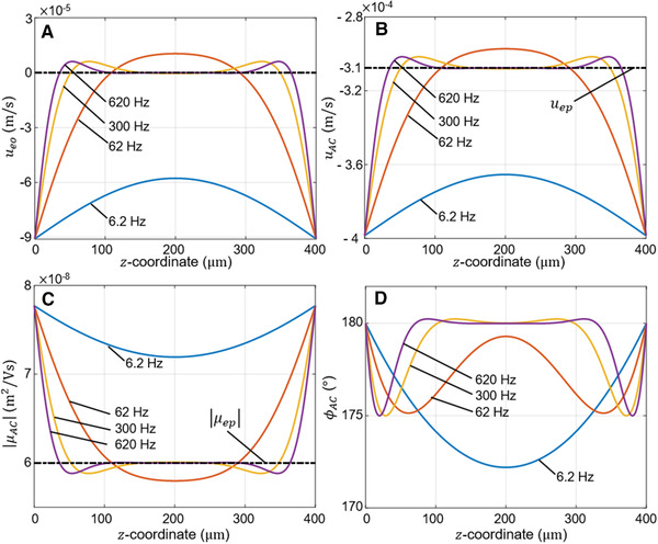
Theoretical profiles of (A) the EOF velocity $u_{eo}$, (B) the particle velocity $u_{AC}$ and (C,D) magnitude $|{\mu }_{AC}|$ and phase ${\varphi }_{AC}$ of the complex AC particle mobility ${\mu }_{AC}$, as a function of the $z$‐coordinate of the microchannel for different frequencies $f_s$. The electrophoretic velocity $u_{\mathrm{ep}}=-3.1\times {10}^{-4}\mathrm{m}/\mathrm{s}$ and the absolute value electrophoretic mobility $|{\mu }_{ep}|$ are represented in dashed lines in (B) and (C), respectively. All plots are computed with the following parameters: ${\mu }_w=-1.8\times {10}^{-8}{\mathrm{m}}^2/\mathrm{Vs}$, $E=5.1\times {10}^3\mathrm{V}/\mathrm{m}$ and ${\mu }_{\mathrm{ep}}=-6\times {10}^{-8}{\mathrm{m}}^2/\mathrm{Vs}$. The frequencies correspond to $f_{\mathrm{s}}=0.1f^{\ast }=6.2\mathrm{Hz},f_{\mathrm{s}}=f^{\ast }=62\mathrm{Hz},f_{\mathrm{s}}=4.8f^{\ast }=300\mathrm{Hz}\mathrm{and}{f}_{\mathrm{s}}=10f^{\ast }=620\mathrm{Hz}$.

According to the results displayed in Fig. 2A, for low frequencies (i.e., $f_{\mathrm{s}}=0.1f^{\ast }$) there is a considerable EO velocity at all $z$ positions, while for frequencies higher than $f^{\ast }$the EOF in the centre of the channel is practically zero. This can be physically understood because the electric field is changing its direction so fast that the liquid flow cannot respond fast enough to develop across the entire channel [19, 21]. In Fig. 2B and C, we can clearly see the consequence of this: at about half the height the channel (i.e., near $z=200$μm) for $f_{\mathrm{s}}=10f^{\ast }$ the velocity of the particle equals the electrophoretic velocity, therefore the measured mobility in this region is equal to the electrophoretic mobility of the particle. Fig. 2D shows the phase of the complex AC mobility ${\varphi }_{AC}$ (see Fig. 1C), which represents the phase of the particle velocity compared to the applied AC electric field. At the midplane of the channel, where the EOF has become practically zero, ${\varphi }_{AC}$ will indicate the sign of the charge of the particle. In Fig. 2D we can see that the particle is out of phase with the external $E$ field, i.e., ${180}^{\circ }$, suggesting that the particle is negatively charged as expected.

The minimal value of $f_{\mathrm{s}}$ required to minimize EO to a desired degree mainly depends on the aspect ratio of the channel and viscosity of the fluid. For example, for a microchannel filled with water and with dimensions as specified above, but with a smaller height $h$, the minimal frequency to avoid EO becomes higher since $f^{\ast }$ increases. Such as for $h=100\mu \mathrm{m}$ the characteristic frequency is $f^{\ast }\approx 1\mathrm{kHz}$ and so $f_s\approx 5\mathrm{kHz}$ is required to minimize EO in a region of $20\mu \mathrm{m}$ near the midplane of the channel. One should also bear in mind that for a higher AC frequency as well as for particles with a very low charge, the particle displacements by electrophoresis are shorter. In such cases, due to measurement errors, it may not be possible to extract the electrophoretic mobility with satisfying accuracy. In our experiments, we opted for an AC frequency $f_{\mathrm{s}}=300\mathrm{Hz}$, almost five times higher than $f^{\ast }$. In Fig. 2A, one can see that for $f_s=300\mathrm{Hz}$ the influence of EO is reduced in a region of $80\mu \mathrm{m}$ wide near the middle of the channel. As will become clear below, to achieve accurate measurements in practice, the frequency of the applied voltage should remain below the frame rate of the camera. Since in this work, the aim is to obtain an accurate value of the electrophoretic mobility ${\mu }_{ep}$, we shall focus in the next section on the region near the middle of the channel where the electroosmotic contribution is negligible at high AC frequencies. In this study, we named the plane in the middle of the channel where we can directly measure ${\mu }_{ep}$the M‐plane (see Fig. 1B), and for our microchannel this corresponds to $z=200\mu \mathrm{m}$.

Note that the presented model is not applicable for rectangular microchannels having different zeta potentials at the different surfaces, e.g., when the channel is made from different materials, and for closed microchannels.

Quite recently, considerable attention has been paid to nonlinear effects in electrophoresis measurements when manipulating highly charged particles or when working at high electric fields strength [22, 23]. For submicron particles in applied electric fields in the order of $\mathrm{kV}/\mathrm{c}\mathrm{m}$, nonlinear velocity components can be present and consequently the model and the method from this work would need to be addressed for this phenomenon. Even though some of the particles used in our experiments are relatively highly charged, since the applied electric field is rather small (in the order of $10\mathrm{V}/\mathrm{cm}$) the observed velocity is expected to depend linearly on the applied field [22].

2.3. Determination of the AC complex mobility

To determine the mobility from the measured particle position, the problem can be conveniently studied in the Fourier space. Let us first evaluate the case of a continuous (non‐sampled) motion of a particle in an AC electrophoresis experiment. In our experiments a sinusoidal electric field $E(t)=E_x\sin ({\omega }_{\mathrm{s}}t)$ is applied in the axial direction of the microchannel. As a result, the x‐position of the particle of interest starts oscillating along the channel with an AC velocity given by Eq. (6), but adding the complex value $-i$, because we apply a sine instead of the cosine:

$$u_{AC}\left(z,t\right)=\mathrm{Re}\left\{-i·{\mu }_{AC}{E}_x{e}^{i{\omega }_{\mathrm{s}}t}\right\}$$ (7)

where Re stands for the real part. The Fourier Transform (FT) of the AC velocity $u_{AC}$, evaluated at the frequency $\omega ={\omega }_s$of the applied field and calculated for a total time $T$ chosen to be an exact multiple of the period of the applied sinusoidal voltage, reduces to:

$${\widehat{u}}_{AC}\left({\omega }_s\right)=\frac{1}{T}\underset{0}{\overset{T}{\int }}{u}_{AC}{e}^{-i{\omega }_{s}t}dt=-i\frac{{\mu }_{AC}{E}_x}{2}$$ (8)

Since our microscopy method determines the position $x(t)$ of the particle, we are interested in the relation between the complex mobility ${\mu }_{AC}$ of the particle and its position. Because the speed is the derivative of the position, we can write ${\widehat{u}}_{AC}=i\omega {\widehat{x}}_{AC}$, and from Eq. (8) we find that the FT of the position evaluated at $\omega ={\omega }_s$becomes:

$${\widehat{x}}_{AC}\left({\omega }_s\right)=-\frac{{\mu }_{AC}{E}_x}{2{\omega }_{\mathrm{s}}}$$ (9)

From Eq. (9) the complex AC mobility can be obtained by:

$${\mu }_{AC}=-\frac{2{\omega }_{\mathrm{s}}}{E_x}{\widehat{x}}_{AC}\left({\omega }_{\mathrm{s}}\right)$$ (10)

If the conditions mentioned in Section 2.2 are satisfied, then the electroosmotic mobility is zero and the electrophoretic mobility ${\mu }_{ep}$ is directly obtained from Eq. (10). In practice, the motion due to EP and EO is superposed with the random Brownian motion such that the FT of the position of the particle at the frequency is $\widehat{x}({\omega }_s)=\widehat{x}{}_{AC}({\omega }_s)+{\widehat{x}}_{BM}({\omega }_s)$. The FT of the position for a freely diffusing particle during a time $T$ is given by [24]:

$${\widehat{x}}_{BM}\left(\omega \right)=-\frac{i}{\omega }\sqrt{\frac{2D}{T}}\widehat{\eta }\left(\omega \right)$$ (11)

Here, $D$ is the diffusion coefficient of the particle and $\widehat{\eta }(\omega )$ is a complex random variable with properties $⟨\widehat{\eta }(\omega )⟩=0$, $⟨|\widehat{\eta }(\omega ){|}^2⟩=1$. The real (Re) and imaginary (Im) parts of $\widehat{\eta }(\omega )$ are independent and uncorrelated variables with a gaussian distribution and with $⟨|\mathrm{Im}\{\widehat{\eta }(\omega )\}{|}^2⟩=⟨|\mathrm{Re}\{\widehat{\eta }(\omega )\}{|}^2⟩=1/2$. Considering that the expectation value of Brownian noise is zero ( $⟨{\widehat{x}}_{BM}(\omega )⟩=0$), the expectation value of $\widehat{x}({\omega }_s)$ still corresponds to the expectation for pure electrophoresis: $⟨\widehat{x}({\omega }_s)⟩=\widehat{x}{}_{AC}({\omega }_s)$. As a result, the expectation value of $-\frac{2{\omega }_{\mathrm{s}}}{E_x}\widehat{x}({\omega }_s)$ is equal to ${\mu }_{AC}$, demonstrating that it is a good estimator for the complex mobility of the particle. This conclusion remains also in the case of additional error contributions as long as, like Brownian motion, these errors have an expectation value of zero.

3. Material and methods

3.1. Experimental apparatus and method

The experimental setup shown in Fig. 3 consists of a custom‐built inverted microscope with a 40x objective (Nikon) and a high‐speed CMOS camera (Zyla 4.2 sCMOS, Andor Instruments) which is externally triggered by a NI‐DAQ (USB‐6363) device. A green LED (M530L3, Thorlabs, 530 nm) is used for bright field illumination. An aperture and a field diaphragm are used to set up Kohler illumination. Particles are dispersed in a commercial microchannel (uncoated #1.5 μ‐Slide VI 0.4, ibidi GmbH). The geometry of the channel is depicted in Fig. 1A. Each microchannel has a height of $400\mu \mathrm{m}$ and a width of $3.8\mathrm{mm}$. The distance between the two reservoirs, which are the inlet and the outlet of the channel, is $17\mathrm{mm}$. Platinum electrodes (World Precision Instrument), inserted in the reservoirs, are used to apply an AC electric field. A sinusoidal voltage generated using an NI‐DAQ and amplified 10 times is applied across these electrodes. The slide with the microchannel is mounted on a 3D piezo nano‐positioning stage (TRITOR 102SG, Piezosystem Jena) for fine adjustments and a vertical axis micro stage (MVS010/M, Thorlabs) and a 2D micro stage (Thorlabs) for coarse motion in the $z$‐ and ($x,y$ )‐directions, respectively. Custom software (LabVIEW) is written to control some of the mentioned equipment, to set the specific parameters for each experiment, to ensure synchronization between the image acquisition with the output voltage and to record all the acquired data.

Figure 3.

(A) Schematic illustration of the experimental setup. (B) The synchronization scheme between the external trigger of the camera, the applied voltage for the channel electrodes and the voltage for the LED. In the synchronization phase, starting at “SYNC”, the LED blinks so that in post‐processing, frame 1 can be identified. While the particle position is initially only subjected to Brownian motion, at “START” the particle begins to oscillate because of the AC field. The camera has an exposure time $t_{exp}$, such that the particle image and the resulting particle position is averaged over the exposure window.

The experimental procedure consists of loading the channel ($30\mu \mathrm{L}$) with a highly diluted particle dispersion. Next, the device is mounted onto the microscope stage and the Platinum electrodes are inserted. In the ($x,y$)‐plane, the microscope is positioned at the centre of the channel ($2\mathrm{mm}$from the edges in the $y$‐direction and about $8\mathrm{mm}$ from the channel ends in the $x$‐direction). The bottom of the channel ($z=0$) is found by using a green laser that is coupled to the back of the objective. If the laser is focused on the bottom surface of the channel its reflection results in a focused spot on the camera. Then, the vertical micro stage is used to bring the focal plane to a desired reference height. In this way, a reference position is obtained. Then, using the piezo stage with a range of $100\mu \mathrm{m}$ in three directions, individual particles can be brought into focus and in the center of the camera field of view of $15\mu \mathrm{m}\times 15\mu \mathrm{m}$. When a particle is in focus and centered in the image, the sinusoidal electric field is applied, and the motion of the particle is recorded at a camera rate of $f_{\mathrm{cam}}=850\mathrm{Hz}$. Measurements last for about $1.5$ seconds per particle. This corresponds to about $1300$ frames per particle. After each measurement, the objective is shifted in the ($x,y$)‐plane to find another particle.

In the present work, two types of experiments are carried out. In the first type, particle mobilities are measured as a function of the $z$‐coordinate for two sets of applied peak voltages and frequencies, namely $V_{AC}=70\mathrm{V},f_{sin}=50\mathrm{Hz}$ and $V_{AC}=80\mathrm{V},f_{sin}=300\mathrm{Hz}$. To characterize the electric field inside the ibidi microchannel, a 3D simulation in COMSOL was ran. The electric field in the channel, far enough from the inlet and outlet, can be considered homogeneous and equivalent to a conducting material between two parallel electrodes separated by $15.6\mathrm{mm}$. Considering this effective length, the peak electrical fields strengths are $4.5\times {10}^3\mathrm{V}/\mathrm{m}$ and $5.1\times {10}^3\mathrm{V}/\mathrm{m}$, respectively. The aim of these measurements is to verify if the dependency of the mobility on the $z$‐position and the frequency corresponds to the theory. In the second type, only particles near the M‐plane of the channel, i.e., at to $200\mu \mathrm{m}\pm 40\mu \mathrm{m}$, are measured. As explained, under these conditions electroosmosis is suppressed, allowing to directly extract the electrophoretic mobility.

The particles studied are the following: $1.9\mu \mathrm{m}$ diameter polystyrene (PS) microspheres from Polysciences, $1.12\mu \mathrm{m}$ diameter polystyrene microspheres functionalized with amino groups on the surface (amino‐PS) from Spherotech, $655\mathrm{nm}$ diameter melamine resin particles (MF) from particles GmbH, and $500\mathrm{nm}$ diameter iron oxide particles (IO) from Ocean NanoTech.

In Fig. 3B, the timing of the experiment is explained. The external trigger for the camera, the voltage applied to the microchannel electrodes, and the driving voltage of the LED are synchronized. To identify frame number 1 a synchronization sequence is used in which the LED blinks before the sinusoidal voltage is applied.

3.2. Experimental analysis

In our experiments, data are recorded for each particle for a time $1.5\mathrm{s}$. When the sinusoidal voltage is applied, the electrophoretic velocity practically immediately reaches a steady state while the electroosmotic velocity is expected to reach a periodic regime after a characteristic time of $16\mathrm{ms}$. In the experiments, this transient behavior was evaluated and compared in amplitude and phase with the rest of the measurement. Since no significant difference was identified and ${\tau }_{eo}\ll T$, this transient phase is ignored, meaning that all data collected in the measurements from the moment the field is applied is used in the analysis.

3.2.1. Determining the particle centroid

The acquired images are analyzed employing a customized MATLAB code. First, the first image after the AC voltage is applied is identified based on the information from the LED synchronization. Next, the particle is located by calculating the center of high radial symmetry. This gives a first estimation of the particle position ($x_1,y_1$). Using ($x_1,y_1)$as initial guess, a box of $31\times 31$ pixels (corresponding to $4.6\times 4.6\mu \mathrm{m}$), containing a boundary of $5$ pixels or $0.75\mu \mathrm{m}$ wide, is centered on the particle. After applying a Gaussian filter, the background $I_{bg}$ is calculated as the average intensity of the boundary. This background value is subtracted from the cropped image. To avoid negative intensities the absolute value is taken. To exclude as much image noise in the background as possible, the centroid algorithm is accompanied by a thresholding procedure. All pixels with a value lower than the threshold, set at $1/3$of the peak intensity, are assigned a pixel value of $0$. Then, the position of the particle ($x,y$) is computed by finding the centroid (center of mass) of the resulting intensity distribution. With $I$ representing the matrix of the resulting pixel intensities of the cropped image, the centroid along the x‐axis is given by:

$$x=\frac{{\sum }_i{\sum }_j{x}_i·I_{ij}}{{\sum }_i{\sum }_j{I}_{ij}}$$ (12)

where $x_i$ is the coordinate of the i‐th pixel on the x‐axis, and $I_{ij}$ is the pixel intensity at the position $(i,j)$ of the image. The y‐centroid can be found in a similar manner. For each particle, a total number of samples $N$ of the particle position, i.e., $x=x(t_n)$ and $y=y(t_n)$, is collected. Since the triggering or sample frequency is $f_{cam}$, the time step between two acquired images is $\mathrm{\Delta }t=1/f_{cam}$.

3.2.2. Time correction

Knowing the precise timing of each recorded particle position is crucial for analyzing the phase of the complex mobility. However, using the timing of the trigger pulse does not provide enough accuracy in the timing of each position measurement. To obtain a satisfying timing three types of time‐delay are considered: the start delay, the exposure time delay, and the rolling shutter delay. The start delay, ${\tau }_S,$ is the time difference between the start of the external trigger pulse of the camera and the start of the exposure. This was experimentally determined as $37.5\mu \mathrm{s}$. The exposure time delay, ${\tau }_E$, arises from the fact that the camera acquires an image of the particle during the time when the image is exposed (see Fig. 3B). We assume that the time associated with an image is set in the middle of the exposure window, i.e., a time${\tau }_E=t_{exp}/2$ after the start of the exposure. In our experiments, the exposure time is $t_{exp}=0.6\mathrm{ms}$, corresponding to ${\tau }_E=0.3\mathrm{ms}.$The rolling shutter delay,${\tau }_R$, is a result of the sequential exposure of horizontal pixel lines in the vertical direction of the camera, see Fig. 4A, starting from the middle towards the sides of the detector. Each row is subjected to the same exposure time, i.e., $0.6\mathrm{ms}$, but with a $9.60\mu \mathrm{s}/\mathrm{row}$ delay compared with the center row at $y=Y_{1/2}$ (see Fig. 4A). This means that the central time of the exposure depends on the y‐coordinate of the pixel. Taking this into consideration, the time $t_n$ associated to a particle with position $(x,y)$ in the image with frame number $n$ is given by:

$$t_n^{\ast }\left(y\right)=n\mathrm{\Delta }\mathrm{t}+{\tau }_E+{\tau }_S+\left(\left|y-Y_{1/2}\right|\right){\tau }_R$$ (13)

with ${\tau }_E=300\mu \mathrm{s},{\tau }_S=37.5\mu \mathrm{s}$, ${\tau }_R=64\mu \mathrm{s}/\mu \mathrm{m}$ and $(y-Y_{1/2})$ the distance from the central row. Notice that the direction of the electric field ($x$‐direction) was chosen to be orthogonal to the direction of the rolling shutter, to minimize the magnitude of the correction.

Figure 4.

(A) A typical image of a $1.9\mu \mathrm{m}$ diameter PS particle, indicating the rolling shutter direction of the camera. (B) Scheme illustrating the time correction algorithm: $N+1$ samples of the $x$‐position acquired with sample frequency $f_{cam}=1/\mathrm{\Delta }t$ (solid dots), and samples with the corrected time (empty dots) according to Eq. (13). The interpolated position$x_M$ at time $t_M^{\ast }$ is shown for the case $t_N^{\ast }<t_M^{\ast }<t_{N+1}^{\ast }$. (C) $x$ and $y$ position of a $1.9\mu \mathrm{m}$ PS particle oscillating in a $300\mathrm{Hz}$ AC field along the $x$‐axis ( $V_{AC}=80\mathrm{V}).$There is a contribution from Brownian motion in both the $x$‐ and $y$‐ directions. (D) Power spectrum $|{\widehat{x}}_k{|}^2$ of the particle in (C) for frequencies below the Nyquist frequency. At $f_k=f_{\mathrm{s}}=300\mathrm{Hz}$ a single peak emerges about 3 orders of magnitude above the Brownian noise. As a guide to the eye, the solid line indicates the expected trend of the power spectrum of Brownian motion. The horizontal dotted line corresponds to the noise level related to particle detection, obtained from measuring a fixed particle.

3.2.3. Experimental determination of the AC mobility of a particle

In this section, we explain how to extract the complex AC mobility from the experimental data of the position of the particle. Experimentally, we sample the position of the particle $x_n$ at a frequency $f_{cam}$. As a result of the time delays considered in the Section 3.2.2, the position $x_n=x(t_n^{\ast })$ is non‐uniformly sampled in time, and the time between consecutive measurements is not exactly $\mathrm{\Delta }\mathrm{t}$ (see Fig. 4B). To determine the complex components of the FT of the position, we approximate the convolution integral:

$${\widehat{x}}_k=\frac{1}{T}\underset{t_1^{\ast }}{\overset{t_1^{\ast }+T}{\int }}x\left(t\right)e^{-i{\omega }_{k}t}dt$$ (14)

by a discrete sum over the data points while taking the appropriate time interval associated with each sample:

$$\begin{array}{ccc}\hfill {\widehat{x}}_k& =& \left[x_1{e}^{-i{\omega }_k{t}_1^{\ast }}\right]\frac{t_2^{\ast }-t_1^{\ast }}{2}+\sum _{n=2}^{N-1}\left[x_n{e}^{-i{\omega }_k{t}_n^{\ast }}\right]\frac{t_{n+1}^{\ast }-t_{n-1}^{\ast }}{2}\hfill \\ & & +\left[x_M{e}^{-i{\omega }_k{t}_M^{\ast }}\right]\left[\frac{t_N^{\ast }-t_{N-1}^{\ast }}{2}+\left(t_M^{\ast }-t_N^{\ast }\right)\right]\hfill \end{array}$$ (15)

where ${\omega }_k=2\pi k/T$ with $k=0,\dots ,N-1$. The last point $x_M$ is linearly interpolated between $x_N$ and $x_{N+1}$ for the time $t_M^{\ast }=t_1^{\ast }+T$. The more measurement points are evaluated, the closer the discrete FT is expected to be to the continuous integral. However, for periodic functions and provided that the number of samples $N$ is sufficiently large, or in other words if $f_{\mathrm{cam}}\gg f_{\mathrm{s}}$, a good agreement between both FTs exists. Therefore, similar as for the continuous theory in Section 2.3, here the complex mobility ${\mu }_{AC}$ is estimated by evaluating Eq. (16) at $k={\omega }_{s}T/2\pi \equiv s$:

$${\mu }_{AC}\cong -\frac{2{\omega }_{\mathrm{s}}}{E_x}{\widehat{x}}_s$$ (16)

The result from Eq. (16) must further be corrected by dividing by a factor $\mathrm{sinc}(\omega t_{exp}/2)$. This correction is related to the effect of the finite exposure window in the value of the position. In Section 3.2.2, the time is corrected assuming that the image was acquired in the middle of the interval $t_{exp}$, hence at time $t_n^{\ast }=t_n+t_{exp}/2$. A similar reasoning should be done for the position values, which are in fact average values within the exposure time interval. This procedure is elaborated further in the Appendix.

The complex mobility can also be split up in an amplitude $|{\mu }_{AC}|$ and a phase ${\varphi }_{AC}$, which is useful for avoiding complicated 3D graphs of the complex mobility versus the $z$‐position in the channel. For measurements in which there is no contribution from EO, such that ${\mu }_{AC}={\mu }_{ep}$, the measured complex mobility ${\mu }_{AC}$ will be scattered close to the real axis. For a negatively charged particle ${\varphi }_{AC}\cong {180}^{\circ }$ while for a positively charged particle ${\varphi }_{AC}\cong 0^{\circ }$or ${\varphi }_{AC}\cong {360}^{\circ }$. In this case, the electrophoretic mobility can be estimated directly by taking the real part of the complex mobility:

$${\mu }_{ep}=\mathrm{Re}\left\{{\mu }_{AC}\right\}\cong \mathrm{Re}\left\{-\frac{2{\omega }_{\mathrm{s}}}{E_x}{\widehat{x}}_s\right\}$$ (17)

by considering that the expectation value $⟨\mathrm{Re}\{{\mu }_{AC}\}⟩$ is equal to ${\mu }_{ep}$. The error due to Brownian motion on ${\mu }_{ep}$ can be found by using Eq. (11) and the mentioned statistical properties of Brownian motion:

$${\sigma }_{BM}=\frac{\sqrt{2}}{E_x}\sqrt{\frac{2D}{T}}$$ (18)

4. Results and discussion

4.1. AC electrophoresis measurements at different AC frequencies and z‐positions

We experimentally investigated particle mobilities as a function of the $z$‐position in the channel at two frequencies ($50\mathrm{Hz}$ and $300\mathrm{Hz}$) of the applied electrical field. A batch $1.9\mu \mathrm{m}$ PS particles dispersed in deionized water are measured between$z=0\mu \mathrm{m}$ and $z=250\mu \mathrm{m}$. Each particle is measured once at these two frequencies, and about 30 different particles were measured. The dependency of the amplitude and phase of the complex mobility of the particles on the $z$‐coordinate is shown respectively in Fig. 5A and B. From Fig. 5A we can see that the amplitude of the complex mobility is high ($|{\mu }_{\mathrm{AC}}|\approx 6\times {10}^{-8}{\mathrm{m}}^2/\mathrm{Vs}$) near the middle of the cell ($z=200\mu \mathrm{m}$), and reduces to a lower value ($|{\mu }_{\mathrm{AC}}|\approx 0.8\times {10}^{-8}{\mathrm{m}}^2/\mathrm{Vs}$) when approaching the bottom wall ($z=0\mu \mathrm{m}$). In the region near the interface between $z=0\mu \mathrm{m}$ and $z=50\mu \mathrm{m}$, $|{\mu }_{AC}|$increases faster for $f_{\mathrm{s}}=300\mathrm{Hz}$ than for $f_s=50\mathrm{Hz}$. This can be understood if we consider the penetration depth $\delta$ which is inversely proportional to the square root of the frequency $f_{\mathrm{s}}$. Thus, for the lower excitation frequency $f_{\mathrm{s}}=50\mathrm{Hz}$ the perturbed region, i.e., ${\delta }_{50\mathrm{Hz}}=80\mu \mathrm{m}$, extends further into the bulk while for the higher frequency $f_{\mathrm{s}}=300\mathrm{Hz}$ the AC disturbance decays considerably faster into the bulk such that a smaller region near the interface is perturbed, i.e., ${\delta }_{300\mathrm{Hz}}=32\mu \mathrm{m}$. For the case of $f_{\mathrm{s}}=300\mathrm{Hz}$, a maximum is observed at about $z=60\mu \mathrm{m}$, and a plateau is reached near the middle of the channel. As explained earlier, this plateau at $f_{\mathrm{s}}=300\mathrm{Hz}$ near the M‐plane of our microchannel, i.e., in a region for $z=200\mu \mathrm{m}\pm 40\mu \mathrm{m}$, is expected because there the EOF becomes negligible, such that the measured mobility becomes equal to the electrophoretic mobility of the particle.

Figure 5.

Amplitude and phase of the complex mobility profiles along the $z$‐axis measured at two frequencies, i.e., $50\mathrm{Hz}$ (circles) and $300\mathrm{Hz}$ (diamonds), of the applied electrical field. In (A, B) for a batch of $1.9\mu \mathrm{m}$ PS microspheres and in (C, D) for a single $1.9\mu \mathrm{m}$PS particle, all dispersed in deionized water. The solid black lines correspond to the best theory fit determined by least squares matching with the following parameters: (A, B) ${\mu }_{\mathrm{ep}}=-5.5\times {10}^{-8}{\mathrm{m}}^2/\mathrm{Vs},{\mu }_w=6.0\times {10}^{-8}{\mathrm{m}}^2/\mathrm{Vs}$ and (C, D) ${\mu }_{\mathrm{ep}}=-4.7\times {10}^{-8}{\mathrm{m}}^2/\mathrm{Vs},{\mu }_w=7.2\times {10}^{-8}{\mathrm{m}}^2/\mathrm{Vs}$. The insets in (C) illustrate the typical case of an isolated PS microsphere (right) and the rare case where the particle is in the neighbourhood of another one resulting in outliers (left).

Next, a comparison between these experiments and the theory is made. The theoretical values for $f_{\mathrm{s}}=50\mathrm{Hz}$ and $f_{\mathrm{s}}=300\mathrm{Hz}$ (solid lines) with two unknown parameters ${\mu }_{ep}$ and ${\mu }_w$ are fitted to the experimental data using a least squares algorithm. The best fit results in ${\mu }_{\mathrm{ep}}=-5.5\times {10}^{-8}{\mathrm{m}}^2/\mathrm{Vs}$ and ${\mu }_w=6.0\times {10}^{-8}{\mathrm{m}}^2/\mathrm{Vs}$. If the Smoluchowski equation would be valid, this value for ${\mu }_w$would lead to a zeta potential of the channel walls of ${\zeta }_w=-85\mathrm{mV}$. Since this exceeds the thermal voltage of ${\varphi }_{th}\approx 25\mathrm{mV}$, this estimation is not acceptable. The zeta potential of the colloidal particles estimated using Helmholtz–Smoluchowski (HS) theory is rather high (in absolute value), i.e., $\zeta =-78\mathrm{mV}$, suggesting that the EDL is considerably polarized and hence that the HS theory is not applicable. In this case, one could use the numerical calculations of O'Brien and White to calculate the zeta potential of the particle [5]. However, since this is out of the scope of this paper, we only refer to the electrophoretic mobility of the particle. For more details on this the reader is referred to [5].

The sign of the electrophoretic mobility is revealed by the phase of the measured mobility at the M‐plane at $f_{\mathrm{s}}=300\mathrm{Hz}$, i.e., ${\varphi }_{AC}\cong {180}^{\circ }$ (see Fig. 5B). As explained above, we can then conclude that the particles are negatively charged, in agreement with the manufacturer's indications. Notice that, while near the center of the channel the particles oscillate in anti‐phase with the electric field, close to the wall the particles oscillate roughly in phase with the electric field, i.e., ${\varphi }_{AC}\cong {360}^{\circ }$. This can be understood from the large contribution of EOF close to the interface, which is in phase with the applied electric field due to the negative surface potential of the channel wall and the associated net positively charged EDL.

The overall trends from both the amplitude and the phase follow the theory well, apart from a small systematic deviation can be observed in the mobility amplitude data. The good agreement confirms that the synchronization of the camera with the AC field and the Fourier analysis of the non‐uniformly sampled data works well. The error associated in the $z$‐coordinate is estimated to be $2\mu \mathrm{m}$. The scattering of the data may include additional error contributions besides Brownian motion. For example, image noise, the accuracy of the intensity centroid, and charge polydispersity within the sample can contribute to the scattering.

To obtain a better idea of the precision of our method, independent from the charge polydispersity of the sample, a single $1.9\mu \mathrm{m}$ PS particle was manually tracked (employing the micro‐ and piezo‐stage) and measured while it was falling by gravity from the middle to the bottom of the cell. The results are shown in Fig. 5C and D. Both the amplitude and the phase of the mobility show a similar trend as that for the batch of particles in Fig. 5A and B. The theoretical match corresponds to ${\mu }_{\mathrm{ep}}=-4.7\times {10}^{-8}{\mathrm{m}}^2/\mathrm{Vs}$ and ${\mu }_w=7.2\times {10}^{-8}{\mathrm{m}}^2/\mathrm{Vs}$.

It has been verified that outliers are caused by the presence of nearby particles as illustrated in the left inset in Fig. 5C corresponding to the value indicated by a circle. For example, due to the presence of neighboring particles, the particle under study may feel an extra drag force which may have an impact in the particle motion. Also, an extra particle in the FOV can cause additional errors in the centroid algorithm.

To evaluate the measurement accuracy, we repeated 10 times the mobility measurement on four different $1.9\mu \mathrm{m}$ PS particles near the M‐plane. The mean electrophoretic mobility ${\mu }_{ep}$ and the standard deviation (SD) for each particle are presented in Table 1. The SD is on the order of 5% of the mean, indicating a satisfying reproducibility. For the case of the $1.9\mu \mathrm{m}$ diameter particles suspended in water and measured in an electric field of amplitude $E_x=5.1\times {10}^3\mathrm{V}/\mathrm{m}$, the error due to Brownian motion, i.e., Eq. (18), is estimated as ${\sigma }_{\mathrm{BM}}=0.2\times {10}^{-9}{\mathrm{m}}^2/\mathrm{Vs}$. The measured standard deviation is about 4 times larger this value, indicating there are other noise contributions.

Table 1.

Mean electrophoretic mobility and standard deviation (SD) for 10 measurements of four different individual $1.9\mu \mathrm{m}$ PS particles, for an applied field with amplitude $5.1\times {10}^3\mathrm{V}/\mathrm{m}$ and frequency $300\mathrm{Hz}$

	Particle 1	Particle 2	Particle 3	Particle 4
mean ${\mu }_{ep}({10}^{-8}{\mathrm{m}}^2/\mathrm{V}\mathrm{s})$	$-2.9$	$-3.8$	$-3.4$	$-3.6$
SD $({10}^{-9}{\mathrm{m}}^2/\mathrm{Vs})$	$0.9$	$0.7$	$1.0$	$0.7$

One type of error is linked to noise in the microscope image, leading to a limited accuracy of the particle position, after application of the centroid algorithm. To estimate this effect, a fixed particle on the bottom of the cell was measured with the same procedure but with no electric field applied, and the FT of the position, i.e., $\widehat{x}$, was found to be independent of the frequency, illustrated by the horizontal line in Fig. 4D. Combining this error amplitude on ${\widehat{x}}_s$ with Eq. (16), the error on the mobility for a $1.9\mu \mathrm{m}$ particle is estimated as ${\sigma }_{\mathrm{cent}\mathrm{roid}}=0.3\times {10}^{-9}{\mathrm{m}}^2/\mathrm{Vs}$, which is larger than the error related to Brownian motion. This noise level depends on the size of the particle and the resolution of the image and may be very important for particles with small mobility.

Another type of error may be due to non‐uniform sampling. The variation in the time step is related to the motion in the $y$‐direction. For the particles with a diameter of $1.9\mu \mathrm{m}$, the time step variation is below 1%, while for the particles with a diameter of $500\mathrm{nm}$ the variation is about 1%, or $0.01\mathrm{ms}$ compared to $\mathrm{\Delta }t=1.2\mathrm{ms}$. Therefore, it seems that the non‐uniform sampling is not important for the noise.

Finally, since the AC frequency $300\mathrm{Hz}$ is relatively close to the Nyquist frequency ($425\mathrm{Hz}$), this may lead to an additional error related to Brownian motion aliasing [24].

It can be noted that there are significant differences in the values of ${\mu }_{ep}$ and the estimated values of ${\mu }_w$ between the single particle from Fig. 5C and D and the measurements from Fig. 5A and B, which can have a number of reasons. Especially the charge stability of the particles over long times plays an important role. We have learned that the procedure of preparing the samples is crucial, and that the average mobility values are sensitive to the age of the sample. For example, the mentioned experiments were reproduced in different days resulting in mobilities varying from about $-3\times {10}^{-8}{\mathrm{m}}^2/\mathrm{Vs}$ to $-5.5\times {10}^{-8}{\mathrm{m}}^2/\mathrm{Vs}$. The outcomes were compared with the commercial apparatus Zetasizer Nano (Malvern). Suspensions in DI water containing the same concentration of $1.9\mu \mathrm{m}$ PS particles were carefully prepared and measured in the Zetasizer Nano. For each sample, three runs were recorded, and the average result was taken. A fresh sample, made and measured on the same day, resulted in a mobility $(-5.1\pm 0.14)\times {10}^{-8}{\mathrm{m}}^2/\mathrm{Vs}$. The same sample measured after $2\mathrm{h}$ gave an electrophoretic mobility of $(-4.2\pm 0.04)\times {10}^{-8}{\mathrm{m}}^2/\mathrm{Vs}$. A sample that was prepared two days earlier resulted in $(-2.9\pm 0.11)\times {10}^{-8}{\mathrm{m}}^2/\mathrm{Vs}$. The results obtained with the camera‐based experiments, e.g., from Table 1 and Fig. 5, fall within the same range determined with the Zetasizer and therefore the absolute values are comparable.

In this context, it is useful to mention that the zeta potential is very sensitive to any level of impurities in the solution or channel walls, and that this can explain some variation in the observed values of the mobility ${\mu }_w$.

4.2. Electrophoretic mobility of a sample containing positively and negatively charged particles

Next, we study the electrophoretic mobility of $1.12\mu \mathrm{m}$ amino‐PS microspheres diluted in deionized water. Following the experimental method explained above, 14 different particles were measured near the M‐plane ($z=200\mu \mathrm{m}\pm 40\mu \mathrm{m}$) using an electrical field with a frequency of $300\mathrm{Hz}$. The amplitude and phase of the complex mobilities are shown in Fig. 6A and B, respectively. The average value of the electrophoretic mobility is ${\mu }_{\mathrm{ep}}=1.9\times {10}^{-8}{\mathrm{m}}^2/\mathrm{Vs}$, with a standard deviation of $0.43\times {10}^{-8}{\mathrm{m}}^2/\mathrm{Vs}$. The phase of the complex mobility is about $0^{\circ }$, which indicates that the particles are positively charged. This was expected since the amino groups are typically positively charged in DI water. The measured standard deviation is much larger than the estimated error due to Brownian motion ($0.2\times {10}^{-9}{\mathrm{m}}^2/\mathrm{Vs}$), which suggests that the amino‐PS particles have a polydisperse electrophoretic mobility.

Figure 6.

Absolute value of the amplitude (A) and phase (B) of the electrophoretic mobility measured for a batch of $1.12\mu \mathrm{m}$ amino‐PS microspheres diluted in deionized water. In the inset in (B) a typical image of a single amino‐PS particle is shown.

A second sample, consisting of a mixture (ratio 1:1) of $1.9\mu \mathrm{m}$ PS and of $1.12\mu \mathrm{m}$ amino‐PS was investigated following the same protocol. The amplitude versus the phase of the complex mobility for a number of different particles is shown in Fig. 7A. Two groups of particles can clearly be distinguished: a group of positively charged particles with phase near $0^{\circ }$ with mean amplitude and standard deviation of the complex mobility $(1.4\pm 0.24)\times {10}^{-8}{\mathrm{m}}^2/\mathrm{Vs}$, and a group of a negatively charged particle with phase near ${180}^{\circ }$ with mean amplitude and standard deviation of the complex mobility $(3.6\pm 0.32)\times {10}^{-8}{\mathrm{m}}^2/\mathrm{Vs}$. These two groups correspond to the amino‐PS particles and PS particles, respectively. This is visually confirmed by observing that the largest particles of $1.9\mu \mathrm{m}$ show more diffraction rings than the smallest particle of $1.12\mu \mathrm{m}$, as can be verified from the inset pictures in Figs. 5C and 6B. Therefore, this result demonstrates the ability of this method to distinguish different types of particles in polydisperse samples based on their electrophoretic mobility. The mobilities are slightly different from the ones found in the separate PS and amino‐PS suspensions, which may be explained by a chemical interaction between the particles.

Figure 7.

(A) Amplitude versus phase of the complex mobility for a sample consisting of a mixture of $1.12\mu \mathrm{m}$ amino‐PS and of $1.9\mu \mathrm{m}$ PS particles. The two samples are clearly separated by their different phase (0° and 180°). The mean electrophoretic mobilities of the amino‐PS and the PS particles are $1.4\times {10}^{-8}{\mathrm{m}}^2/\mathrm{Vs}$ and $-3.6\times {10}^{-8}{\mathrm{m}}^2/\mathrm{Vs}$, respectively. (B) Electrophoretic mobility, i.e., ${\mu }_{ep}=\mathrm{Re}\{{\mu }_{AC}\}$, measured near the M‐plane for different types of particles in DI water (from top to bottom): $1.12\mu \mathrm{m}$ amino‐polystyrene particles (asterisks), $655\mathrm{nm}$ melamine resin particles (circles), $500\mathrm{nm}$ iron oxide particles (diamonds) and $1.9\mu \mathrm{m}$ polystyrene particles (squares).

Next, we further evaluate how well our method can distinguish dispersions with different particle materials and sizes. We measure the electrophoretic mobilities of three different batches of particles in the middle of the channel at a 300 Hz alternating electric field. The studied particles are: $1.9\mu \mathrm{m}$ PS, $655\mathrm{nm}$ MF and $500\mathrm{nm}$ IO. The particle sets are individually measured in 3 different channels. Fig. 7B shows the electrophoretic mobility ${\mu }_{ep}$ of particles from the mentioned batches as well as the previous results for the $1.12\mu \mathrm{m}$ amino‐PS from Fig. 6A and B. The average electrophoretic mobility values for each batch of particles, the corresponding standard deviation (SD), the expected error due to Brownian motion (${\sigma }_{BM}$) and the error due to image noise in the determination of the centroid (${\sigma }_{centroid}$) are shown in Table 2.

Table 2.

Mean electrophoretic mobility (average of about 12 measurements) and corresponding standard deviation (SD) for the particles shown in Fig. 7B. ${\sigma }_{BM}$ gives the expected error due to Brownian motion on the electrophoretic mobility, i.e., Eq. (18). ${\sigma }_{centroid}$ is the estimated error related to the accuracy in the particle tracking and it is determined by measuring a fixed particle

	PS	Amino‐PS	MF	IO
mean ${\mu }_{ep}$ $({10}^{-8}{\mathrm{m}}^2/\mathrm{Vs})$	$-4.3$	$1.9$	$-1.7$	$-3.1$
SD $({10}^{-9}{\mathrm{m}}^2/\mathrm{Vs})$	$1.8$	$4.2$	$1.0$	$3.3$
${\sigma }_{BM}$ $({10}^{-9}{\mathrm{m}}^2/\mathrm{Vs})$	$0.2$	$0.2$	$0.3$	$0.4$
${\sigma }_{\mathrm{cent}\mathrm{roid}}({10}^{-9}{\mathrm{m}}^2/\mathrm{Vs})$	$0.3$	$0.7$	$1.0$	$2.0$

To estimate the dispersion in the mobility, we must distinguish two cases: when the SD is much larger than the total error (i.e., $\sqrt{{\sigma }_{BM}^2+{\sigma }_{centroid}^2}$) and when the SD is equal or comparable to the total error. For the first case, the polydispersity on the mobility of a set of particles can be estimated by dividing the SD of the mobility (for a set of particles) by the mean value: $\mathrm{SD}/\mathrm{mean}({\mu }_{ep})$. For example, for the amino‐PS and the PS particles we find a polydispersity of 22% and 4%, respectively. For the second case, an accurate determination of the polydispersity is not straightforward, because most of the SD is due to the total error. This is the case for the MF and IO particles.

5. Concluding remarks

In this work, we have carried out accurate measurements of the electrophoretic mobility of individual microparticles by measuring particles in the middle of a microchannel and applying an AC electric field of a high frequency such that EO can be ignored. Similar methods can be found in the literature with distinct advantages and disadvantages, including that developed by Sadek [7], Ikeda [10], or more extensive approaches such as the one presented by Oddy and Santigo [8] in which probability density functions for particle mobilities are reported. Despite sharing some underlying principles, the advantage of our approach is that a single measurement (at a single AC frequency) is sufficient to obtain an accurate value of the electrophoretic mobility including phase information. This is an improvement over existing techniques which rely on multiple measurements (e.g., DC + AC, or multiple AC frequencies) in combination with theoretical models in order to separate the electrophoretic mobility from the electroosmotic mobility, or which rely on a limited number of data points per measurement. The proposed technique relies on synchronization of the camera with the applied AC field and Fourier analysis of the resulting non‐uniformly sampled particle positions. The same technique can also be used to analyse particle mobilities in the presence of electroosmosis, and to characterize the electroosmotic flow itself.

In this study, it is verified that the amplitude and phase of the measured complex mobility of particles as a function of the $z$‐position follow the theoretical expectation. It was confirmed that there is indeed a parameter space at high AC frequencies in the middle of the microchannel where the EOF becomes negligible and where the electrophoretic mobility can be measured directly. Second, a mixture of positively and negatively charged particles is measured. The results show that the method is able of distinguishing the two types of particles: the mobilities are well separated both in amplitude and in phase. Thirdly, to further demonstrate the method, several different particle samples (different materials and sizes) were measured, and it was shown that the different particle samples can be distinguished well based on their electrophoretic mobility.

In addition, we analyzed the most probable source of errors to calculate the electrophoretic mobility, namely the particle tracking uncertainty, the BM noise, the 2D approximation of EOF, the error due to the non‐uniform FT, and the possible aliasing.

Overall, these experiments demonstrate the potential of this method to accurately characterize the electrophoretic mobility of all kinds of particles. Therefore, this method can be used to investigate with high precision dynamic processes occurring on the surface of particles that modify the mobility, such as charging dynamics relevant for electronic inks, or molecular binding events in biosensing applications. Further studies are needed to evaluate the method in different physiological liquids.

We thank Prof. Kevin Braeckmans and the team from the Biophotonics Research Group (Ghent University) for assistance with the Zetasizer measurements and for providing the iron oxide particles. The research of Íngrid Amer Cid is funded by the Research Foundation‐Flanders (FWO) through the Strategic Basic Research grant 1SA5919N.

The authors have declared no conflict of interest.

Amplitude correction

A sinusoidal signal of the form $x(t)=A\cos (\omega t+\varphi )=\mathrm{Re}\{A{e}^{i\omega t+\varphi }\}$ is measured. Since frames are acquired during the exposure time $t_{exp}$, the measured position is an average amplitude with the exposure time such as:

$$x\left(t^{\ast }\right)=\frac{1}{t_{exp}}\underset{t^{\ast }-\frac{t_{exp}}{2}}{\overset{t^{\ast }+\frac{t_{exp}}{2}}{\int }}A\cos \left(\omega t+\varphi \right)dt$$ (A1)

This results in:

$$\begin{array}{ccc}\hfill x\left(t^{\ast }\right)& =& {\displaystyle \frac{1}{t_{exp}}\left[\sin \left(\omega t^{\ast }+\omega \frac{t_{exp}}{2}\right)-\sin \left(\omega t^{\ast }-\omega \frac{t_{exp}}{2}\right)\right]}\hfill \\ & =& {\displaystyle \frac{1}{t_{exp}}\frac{A}{\omega }\left[2\cos \left(\omega t^{\ast }\right)\sin \left(\omega \frac{t_{exp}}{2}\right)\right]}\hfill \\ & =& {\displaystyle A\frac{\sin \left(\omega \frac{t_{exp}}{2}\right)}{\omega (t_{exp}/2)}\cos \left(\omega t^{\ast }\right)}\hfill \end{array}$$ (A2)

Here, we made use of Simpson's formula. The resulting sinusoidal signal has the same phase but a smaller amplitude. To compensate for this, the mobility data must be divided by the constant factor $\mathrm{sinc}(\omega t_{exp}/2)$.

Data availability statement

The data that support the findings of this study are available from the corresponding author upon reasonable request.