H-scan trajectories indicate the progression of specific diseases

Abstract

Purpose:

The ability of ultrasound to assess pathology is increasing with the development of quantitative parameters. Among these are a set of parameters derived from the recent H-scan analysis of subresolvable scattering. The emergence of these quantitative measures of tissue/ultrasound interactions now enables a study of the unique trajectories of multiparametric features in multidimensional space, representing the progression of specific diseases over time. We develop the mathematical and visual tools that are effective for classifying, quantifying, and visualizing the steady progression of several diseases from independent studies, all within a uniform framework.

Methods:

After applying the H-scan analysis of ultrasound echoes, we trained a support vector machine (SVM) to classify the unique trajectories of progressive liver disease from fibrosis, steatosis, and pancreatic ductal adenocarcinoma (PDAC) metastasis. Our approaches include the development of trajectory maps and disease-specific color imaging stains.

Results:

The multidimensional SVM image classification reached 100% accuracy across the three different studies.

Conclusion:

H-scan trajectories can be useful to track the progression of multiple classes of diseases, improving diagnosis, staging, and assessing the response to therapy.

1. INTRODUCTION

The value of tracking ultrasound anatomical measurements over time has been enshrined for decades in the chart of biparietal diameter vs. gestational age, a widely used reference for monitoring the health and growth of the fetus^1–3. An example is shown in Fig. 1.

Figure 1:

A plot of fetal development represented by ultrasound measurement of cranial diameter as a function of time during pregnancy. The blue line represents the mean and the green area represents the 90% prediction interval. By Mikael Häggström, used with permission³.

Over the years, the list of useful anatomical measurements has grown. These are structures that are large enough to be resolved by medical ultrasound scanners and identified over time to assess changes. Examples include the cross sectional area of nerves⁴, cardiovascular and arterial measures^{5, 6}, muscle disease⁷, kidney cysts⁸, and cancer volumes⁹. However, the reproducibility of anatomical measures of 3D anatomy with ultrasound has been limited by user factors and the predominance of 2D imaging systems^{8, 9}. Separately, Doppler ultrasound measurements over time have seen useful applications in a range of conditions, including rheumatoid arthritis, fetal development¹⁰, and cardiovascular diseases^{11, 12}. The majority and the simplest of these measurements involve a single parameter measured at two time points, creating a delta or change (difference) measure. At a higher level of complexity lies the ability to estimate multiple parameters over time^13–16. When extended to subresolvable scattering properties, this enables an assessment of the measured parameters that provide the highest discrimination between groups: for example responders and non-responders to chemotherapy¹⁷; normal and abnormal liver conditions^18–20.

We propose that the diagnostic value of multiparametric ultrasound measures can be advanced by combining the following concepts:

• By applying the H-scan analysis, which is linked to the scattering and wave propagation physics within tissues, and

• by creating trajectories of H-scan (and other) measures in multidimensional spaces, representing the progression of disease or response to treatments, and

• by deriving color-coded images based on proximity to clusters in multidimensional parameter spaces, representing distinct pathological conditions.

In effect, the original concept of the biparietal diameter curve is extended to a higher dimensional space, but with important transformations. First, the simple anatomical measure of size is replaced by advanced metrics related to the biophysics of scattering and wave propagation, representing interactions that occur on a subresolvable scale within conventional imaging systems. Second, the progression of disease or pathology must be mapped out in the multidimensional parameter space and segmented into unique pathways or clusters. Finally, the tools for visualizing, simplifying, and segmenting multiparameter spaces are needed to reduce the dimensionality and make practical visualizations of the results. Among these tools, we find that principal component analysis (PCA) and the support vector machine (SVM) are robust and practicable means to achieve a clinically useful trajectory that can be visualized and used as a diagnostic guide. The importance of the final representation of the measured data cannot be understated; as Tufte says “…certain methods for displaying and analyzing data are more likely to produce truthful, credible, and precise findings. The difference between an excellent analysis and a faulty one can sometimes have momentous consequences²¹.”

2. MATERIALS AND METHODS

In order to classify, quantify, and visualize the steady progression of several diseases from independent studies within a uniform framework, the following experiments were conducted and analyzed.

2.A. Animal models

We investigated three unique diseases of pancreatic ductal adenocarcinoma (PDAC) liver metastasis, fibrosis, and steatosis from separate as in vivo studies. These animal studies are summarized in Fig. 2(a). The PDAC liver metastasis^{22, 23} was developed in 9 mice (C57BL/6J) that were purchased from Jackson Laboratory (Bar Harbor, ME, USA). To grow the tumor in livers, 4 × 10⁵ luciferase expressing murine pancreatic tumor cells (KCKO-luc) were injected into the spleen, and then the tumor cells spread through the hepatic veins, causing metastasis in the liver. The mice were divided into two groups of control (n = 4) and treated (n=5). The treated group underwent chemotherapy with Gemcitabine (50 mg/kg dosing, twice per week). The tumor growth was confirmed by pathology and bioluminescence imaging (BLI). Hematoxylin and eosin (H&E) stained liver sections, provided different colors for normal and tumor cells as shown in Fig. 3(m). According to BLI, all 9 enrolled mice showed an increase in radiance from D-Luciferin as the tumor grows. The PDAC study was approved by the University of Rochester Committee on Animal Resources.

Figure 2:

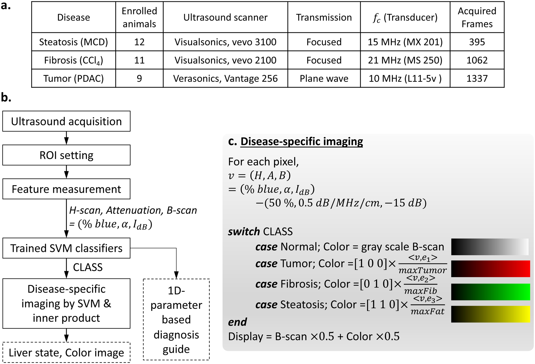
(a) Study design and ultrasound acquisition are summarized. The three disease models were investigated and the number of enrolled animals for each model were provided. Three ultrasound scanners scanned the animals using the transmission beam types with their center frequencies (f_c). Each animal was scanned repeatedly over time to monitor disease progression, and for each scan, several frames were acquired, thereby the total of acquired frames are provided, and these were used for analyses of this study. (b) Flow chart suggesting liver diagnosis guide, including disease-specific imaging and 1D parameter method. First, clinicians would scan a liver and set ROI box. Then features are extracted using H-scan, attenuation estimation, and B-scan procedures. Using the measured features, trained SVM identify liver conditions for all pixels within the ROI, and disease-specific imaging displays color images. Furthermore, using the features, 1D parameter analysis by trained SVM is also performed and help diagnosis based on H-scan trajectories in Fig 5. (c) Detailed color processing for disease-specific imaging. Input for the processing is features and CLASS from the SVM, which are obtained for all pixels within a ROI. A color for each pixel is assigned according to the determined CLASS, and then inner product between feature vector v and unit vector e_n for disease progression direction of the CLASS is performed to calculate color intensity. The unit vectors were also calculated when training SVM using all acquired frames in (a). The colors for PDAC tumor, fibrosis, and steatosis were set as red, green, and yellow, respectively. In this way, the color image is made and transparently overlaid on B-scan, whereas the pixels identified as normal do not have colors, showing only B-scan.

Figure 3:

Disease-specific imaging. (a) 3 features of liver tissues were extracted by H-scan, attenuation estimation, and B-scan, generating the components of (% blue, α, I_dB), respectively. The coordinate represents (H, A, B) = (% blue, α, I_dB) – (50, 0.5, −15) for convenience, meaning changes from normal liver (50%, 0.5dB/MHz/cm, −15dB). Linear lines show disease progression pathways from normal to end time point causing death. All measured features of this study were projected onto their diseases’ pathway, showing scatter plots. The end points causing death are denoted using the symbol “×”. Then the distance between the origin and the measurement can be used for color intensity, meaning the greater value represent more severe disease. SVM classifies liver states, and assigns colors of yellow, green, and red for steatosis, fibrosis, and tumor, respectively. Then, the colors are overlayed on B-scan (b-d, f-h, j-l). Normal in (b, f, j) only shows B-scan without colors. Early stages in (c, g, k) have some color area with low intensity. Late stages in (d, h, l) fill in with saturated colors, representing extensive disease. Pathology slides (e, i, m) shows different cellular patterns for the three disease, supporting the different colors for the three diseases.

The fibrosis was induced in response to carbon tetrachloride (CCl₄) exposure (1mL/kg, three times per week) under approval of Pfizer Animal Care and Use Committee. Eleven rats were enrolled: 7 Sprague-Dawley (SD, Charles River Laboratories, Wilmington, MA, USA) and 4 TAC NIHRNU (nude, Taconic Biosciences, Inc., Rensselaer, NY, USA). After the CCl₄ dosing, an expert pathologist assessed fibrosis response using trichrome stain and Picrosirius red, and all the rats were graded as stage 4 fibrosis. However, since CCl₄ can also cause fat accumulation, we measured the fat area percentage by using Oil Red O stain, resulting in 2.9 ± 1.9 %. To verify the enrolled rats have fibrosis, but minimal fat accumulation, fat area for the other 9 normal SD rats was also measured, resulting in 1.2 ± 1.5 %: p-value comparing the normal and fibrosis group is 0.05.

Regarding the steatosis, a methionine and choline deficient (MCD) diet was employed to activate a nonalcoholic fatty liver disease (NAFLD) model. Twelve SD rats (Charles River Laboratories, Wilmington, MA, USA) were fed the MCD diet (MP Biomedicals, Solon, OH) for 6 weeks. The fat accumulation was assessed by a pathologist using PicroSirius red and H&E. The steatosis study was approved by the Institutional Animal Care and Use Committee at the University of Texas at Dallas.

2.B. Ultrasound data acquisition and experimental set up

Ultrasound scans were performed independently for the three disease models by using three different ultrasound systems; consequently, a total of 2778 ultrasound images were acquired as described in Fig. 2(a). First, a Verasonics ultrasound scanner (Vantage 256, VeraSonics, Inc., Kirkland, WA, USA) equipped with an L11–5v probe at a 10 MHz center frequency imaged the livers with progression of the tumor. Plane wave transmission (25 angles, −6° to 6°) generated IQ data in the Verasonics system. For all of the 9 enrolled mice for the PDAC model, the data acquisition was performed twice a week from day 11 after the tumor cell injection until the death of each mouse; the last scan days range from day 28 to day 64. At each time point for the same mouse, 3 to 5 frames were obtained, resulting in 395 radiofrequency (RF) datapoints. The fibrosis study used a Vevo 2100 (FUJIFILM VisualSonics, Toronto, ON, Canada) with a 21 MHz center frequency linear array transducer (MS 250), of which focused beam transmission acquired RF data once a week from baseline before dosing; the rats survived until 6 or 8 weeks. At each time point for the same rat, approximately 30 frames were obtained, and therefore 1062 scans were acquired. The ultrasound scanner for the steatosis model is Vevo 3100 (FUJIFILM VisualSonics, Toronto, ON, Canada) utilizing a 15 MHz center frequency linear probe (MX 201). RF data acquisition with focused beam transmission was performed at baseline (before starting the MCD diet), week 2, and week 6. For each scan, approximately 30 frames were examined, resulting in 1337 scans.

Using the acquired ultrasound signals, we obtained B-mode images, and then set a ROI for each animal, including a consistent liver area over time for the same animal; example ROIs are provided in Fig. 3 (b–d, f–h, j–l) as the red boxes. The data within each ROI were assigned as inputs for H-scan, attenuation estimation, B-scan, and disease-specific imaging.

2.C. Feature measurement

For each liver, the H-scan % blue, attenuation coefficient α (dB/MHz/cm), and B-scan intensity I_dB (dB) were measured using the H-scan matched filter analysis. In general terms, these parameters pertain to the frequency-dependent transfer function of the tissue scatterers, the frequency dependent attenuation coefficient of the tissue, and the relative scattered intensity, respectively. Specifically, the H-scan % blue reveals differences in transfer functions of scatterers and is implemented using convolution between ultrasound echo r(t) and a matched filter set, including n Gaussian filters $\left\{G_k|\text{exp}\left(-\frac{f-G{C}_k}{2{\sigma }_G{}^2}\right)\text{for} k=1, \dots , n\right\}$ with the Gaussian center frequencies G C_k, but the same band width σ_G. For each time point t, $r\left(t\right)*{\mathcal{F}}^{-1}\left(G_k\right)$ yields n convolution values, that are likely to have a single maximum, indicating any shift in spectrum of the echo signal r(t). Consequently, H-scan analysis can find the spectral shift at each sampling point of RF data by finding the maximum across the convolution results. However, ultrasound propagation causes frequency- and depth-dependent attenuation, resulting in the frequency down shift along with depth. The frequency shift was used to estimate the α:

$$\alpha \left(x\right)= -\frac{f_p\left(x\right)-f_c}{x{\sigma }^2}$$ (1)

where f_p(x) is measured peak frequency (MHz) at depth x (cm). f_c and σ are the center frequency and band width of received echo, respectively, but before attenuation effects; these can be considered as initial parameters. With the estimated α, attenuation correction was performed, producing an attenuation corrected signal r′(t). Next, the convolution $r^{\prime }\left(t\right)*{\mathcal{F}}^{-1}\left(G_k\right)$ then achieves matched filter outputs and corresponding peak frequencies for the points ∈ (Sample, Scanline again, and pseudocolor²⁴ maps the frequency to H-scan color. Since each Gaussian filter has corresponding colors, there are n color levels ranging from red to blue. This study used n = 256, indicating there are 256 color levels; the lower 128 levels from 1 to 128 in sequence represent red colors from vivid to darker, respectively, whereas the higher 128 levels from 129 to 256 represent from dark blue to bright blue. Within ROI of RF data, % blue is defined by:

$$\% \mathit{\text{blue}}=\frac{\left(\mathit{\text{number}} of \mathit{\text{blue}} \mathit{\text{pixels}}\right)}{\left(\mathit{\text{number}} of \mathit{\text{total}} \mathit{\text{pixels}}\right)}\times 100\%.$$ (2)

More details for H-scan analysis including attenuation correction and estimation are found in Parker and Baek²⁵, Baek et al.¹⁶, respectively. The % blue varies according to Gaussian filter parameters of GC_k and σ_G, and therefore we needed to set the parameters with a consistent standard for the three different ultrasound scanners. For the consistent setting, a band width (BW) is defined at 0.3 of normalized frequency spectrum S(f). Each scanner’s {GC_k|k = 1 … 256} of Gaussian filters was set to have % blue = 50% for normal livers, and GC_k=256 – GC_k=1 = 0.7 × BW.

The three ultrasound scanners have different procedures to obtain log-compressed B-mode data, and the B-mode intensity was generally optimized for each scanner. Therefore, for use of I_dB as a feature in addition to % blue and α, the intensity of normal livers was set to −15 dB.

After measuring the features as described above using the 2778 ultrasound scans, the features at the same time point for the same animal were averaged, and therefore we finally obtained 115, 47, and 36 data set for PDAC tumor, fibrosis, and steatosis, respectively, meaning that a total of the 198 averaged data (% blue, α, I_dB) were used for all feature analysis in this paper.

2.D. Non-linear parameter transformation suggesting a combined parameter

We proposed a non-linear transformation to produce a 1D parameter by combining two properties of PCA and the features obtained by H-scan and attenuation estimation. We keep the form of transformation Z = XW from PCA where X and Z are the input and output of PCA, respectively, and W is a weight matrix, but we determine the W based on the H-scan and attenuation results from livers. Normal livers are reported to have approximately 0.5 dB/MHz/cm attenuation and have 50% blue for H-scan measurement. When considering $\left(\% \mathit{\text{blue}}, \alpha \right)\in {ℝ}^2$, measurements from normal livers form clusters around (50, 0.5), and progression of any diseases makes the features (% blue, α) change from the normal values, following a pathway that is unique to the three studied diseases. The parameter changes of Δ(% blue) and Δα indicate the progressions; these two parameters are independently changed according to disease types.

Prior to parameter transformation, including PCA, data normalization is commonly performed such as Z-score or min-max normalization²⁶. To set zero-mean and unit-standard deviation, the normalized parameters x_H and x_A for % blue and α, respectively, are obtained by:

$$x_H=\frac{\left(\% \mathit{\text{blue}}\right)-50}{10}; x_A=\left(\alpha -0.5\right)\times 10$$ (3)

where 50 and 0.5 are the averages of % blue and α, respectively, setting the zero-mean. The scaling operations by 10 serves to set approximately unit-standard deviation and also comparable scales for the different measurements x_H and x_A. Considering PCA with normalized parameters of x_H and x_A, the first principal component PC₁ is:

$$P{C}_1=w_1\cdot x_H+w_2\cdot x_A$$ (4)

where w₁ and w₂ can be positive or negative and are optimized by PCA to maximize the variation of PC₁. However, after examining the way that PCA derives PC₁ in Equation (4) and the particular direction of changes with disease progression, we propose a Combined Parameter C:

$$C= w_H\cdot \left|x_H\right|+w_A\cdot \left|x_A\right|$$ (5)

where w_A = 0.6 sign (x_A) and w_H = 0.4 sign (x_A). Note that both weights rely on the sign of attenuation, making this a nonlinear combination. The weights, 0.4 and 0.6, are optimized contributions from H-scan and attenuation, respectively, to maximize classification accuracy instead of the variance. Note that w_H and w_A can be positive or negative depending on the direction of change of attenuation, as x_A is positive for steatosis but negative for fibrosis and PDAC metastases. Thus, the sign enables better discrimination between steatosis and the other two diseases. Therefore, the C was used for a SVM training to classify liver states.

2.E. SVM learning

The SVM^27–29 is a popular machine learning method related to the maximum margin classifier, which we employed in this study due to advantageous properties. To maximize the margins between distinct classes, the SVM considers those data points located close to class boundaries; these are called support vectors. This is an advantage with a small training data set, since the SVM does not require many data points distant from the class boundaries. Accordingly, we trained two SVM classifiers using 32 animals with 4 liver states: normal, PDAC tumor, fibrosis, and steatosis. All 2778 ultrasound scans in this study were analyzed for values (% blue, α, I_dB, C) , and the features were averaged over frames for the same animal at the same time point, resulting in 198 feature sets for all time points. However, the SVM training used only 64 feature sets which were obtained only from the first and last scans, which are called start and end time points, respectively. The start points were considered as normal livers (n=32), and the end points became disease groups, including steatosis (n=12), fibrosis (n=11), and PDAC tumor (n=9), which were assigned as 4 classes.

SVM implementation was performed using MATLAB (The MathWorks, Inc., Natick, MA, USA). For the classification of the four classes, multiple vs. one method was used, and the Gaussian kernel function was also used to construct smooth hyperplanes. Hence the SVM learning involves the two parameters of box constraint and sigma of the Gaussian, which were optimized to obtain robust hyperplanes, but avoiding overfitting; for the optimization, both hyperplane shapes and classification accuracies were observed by varying the two parameters¹⁶.

Two SVM trainings were performed with 1D (C) and 3D (% blue, α, I_dB) input features to suggest decision boundaries for trajectories based on parameters and images, respectively. When designing a liver diagnosis guide for clinicians with parameters, the simplest way can be providing decision boundaries for the 1D parameter which can be obtained repeatedly over time as the use of biparietal diameter³. Therefore, with the 1D combined parameter, we first trained a 1D SVM classifier producing 1D decision boundaries for liver states.

Moreover, when we try to consider higher dimensional parameters with more information, M-dimensional measurements can also be treated by PCA and SVM. Thus, we suggest a color imaging method with a 3D SVM classifier to effectively reveal and visualize disease trajectories with their decision boundaries; it is also applicable to M > 3. The 3D SVM training requires data normalization to avoid weights for specific features caused by data scales. The scales of each component (% blue, α, I_dB) differ in ranges of [0, 100], [0, 1], [−60, 0], respectively, but % blue and α hardly reach the extremes. (% blue, α × 100, I_dB) is likely to have comparable scales, which were therefore used for the 3D SVM training input and then produced 3D hyperplanes.

2.F. Disease-specific imaging utilizing inner product and SVM

We propose disease-specific imaging to incorporate higher-dimensional features and show their changes using gradual colors, which can effectively visualize 3D feature trajectories caused by disease progressions. A framework for disease-specific imaging is illustrated in Fig. 2(b, c), comprising the following steps: (1) Ultrasound data acquisition for a liver; (2) Feature measurements (% blue, α, I_dB); (3) SVM classification for the input liver; (4) Color processing utilizing the SVM and inner product; (5) Display of disease-specific images, identifying the liver state.

When training the SVM, we also performed a pre-processing for the inner-product-based color processing to obtain pathways of disease progressions in 3D space. The SVM trainings used 64 data at start and end time points, whereas the inner product operation employed features at all time points, consisting of 198 data of (% blue, α, I_dB). Using the 3D features, we define a vector v suggesting disease progression directions starting from a position N of normal liver:

$$v=\left(H,A,B\right)=\left(\% \mathit{\text{blue}}, \alpha , I_{dB}\right)-N$$ (6)

where N = (50%, 0.5 dB/MHz/cm, −15 dB), and (H, A, B) represents feature changes from normal. When monitoring the vector v of a liver from normal state until any disease progresses, v starts from the origin of O = v = (0, 0, 0) and repeated measurements over time move gradually further from the origin O. Then, the trajectories of v indicate disease progression pathways and also directions of progression. By collecting v for each disease, linear pathways of tumor, fibrosis, and steatosis can be obtained by linear fittings; the lines are shown in Fig. 3(a). Furthermore, the progression directions for tumor, fibrosis, and steatosis can be also estimated by calculating unit vectors of $\widehat{e_1}$, $\widehat{e_2}$, and $\widehat{e_3}$, respectively. Then, an inner product given by $v\cdot \widehat{e_n}$ indicates progression of n-th disease, and the values $v\cdot \widehat{e_n}$ for all enrolled 198 data are exhibited in Fig. 3(a) as points with colors representing disease stages: the darker and brighter colors represent early and late stages of each disease, respectively, until the time of death given by the symbol “×”. Among the 198 projections onto the linear pathways, maximum values of the diseases were obtained: $\mathit{\text{maxTumor}}=\text{max}\left(v\cdot \widehat{e_1}\right), \mathit{\text{maxFib}}=\text{max}\left(v\cdot \widehat{e_2}\right)$, and $\mathit{\text{maxFat}}=\text{max}\left(v\cdot \widehat{e_3}\right)$ for tumor, fibrosis, and steatosis, respectively. The maximum values normalize the inner product results, and then as described in Fig. 2(c), the normalized values of $\frac{\langle v,\widehat{e_n}\rangle }{max{\left(\mathit{\text{Disease}}\right)}_n}$ are assigned for RGB color intensity for each pixel, wherein v is a measurement from any pixels within the ROI and the disease index of n is determined by the trained 3D SVM classifier. The normalized value utilizing inner product and SVM indicates disease progression; the higher the value, the more severe the disease, but values near 0 indicate normal or early stages. In this way, a color image is processed, and then overlaid with its B-scan; pixels classified as normal only display B-scan without color overlay.

3. RESULTS

We present results obtained from three different animal models of disease, each study utilizing its own ultrasound scanner acquiring in vivo data. These are: a liver fibrosis model, a liver steatosis model, and a PDAC metastatic model. The disease trajectories are based on H-scan analysis with three output parameters (% blue, α, I_dB) related to the upshift in scattering, the acoustic attenuation, and the B-scan echo intensity from regions within the liver, as described in the Methods section.

3.A. Trajectories in low dimensional spaces

Perhaps the most simple and traditional approach is measuring and plotting each measured parameter individually over time. For example, the progression of PDAC liver metastasis was found to produce changes in H-scan measures over time in days, indicating tumor growth as shown in Fig. 4. Specifically, the % blue parameter in Fig. 4(a) shows a gradual increase over time for both the untreated and treated (with chemotherapy) mice, but the chemotherapy group tends to have an increase in survival compared to the untreated group. When considering only start and end points, the percent difference is significantly different with p-value of 5.7 × 10⁻⁶. Moreover, we estimated the attenuation coefficient α using the H-scan approach by measuring frequency down-shift along with depth, and Fig. 4(b) demonstrates that the α can decrease with gradual tumor growth over time. The start and end points show significant difference (p-value = 3.6 × 10⁻¹⁰) without any overlap between the measurements of the two groups. Whereas, the difference between the start and end points investigated by traditionally used B-scan intensity has a p-value of 0.01, which is statistically significant, but less significant than that of H-scan % blue or α. Thus, H-scan % blue and attenuation estimation more sensitively describe the changes induced by the tumor compared to B-scan. In Fig. 4(c,d), we combine the three metrics to make a joint assessment of the three, and therefore considered three dimensional (3D) features for each liver and time point, (% blue, α, I_dB). The gradually changed red colors from dark to bright red in Fig. 4(d) illustrate start-to-end time points, representing liver changes from normal to an end-stage metastatic condition causing death. The trajectories in the plot of Fig. 4(c) suggest a common pathway of tumor growth. To be specific, scatterers with features (% blue, α, I_dB) located near front left can be considered as late stage tumor.

Figure 4:

H-scan trajectories indicating the progression of PDAC tumor metastasis. H-scan analysis extracted two features within liver tissues, which are blue percentage (a) and attenuation coefficient (b) along with time, representing days after tumor injection. The feature measurements were performed from start points (•) to end points (×), representing early and late stage causing death, respectively. The blue percentage (a) and attenuation (b) gradually increase and decrease over time, respectively, as tumor progresses. The features show significant between the early and late stages, and “****” denotes p-value < 0.0001. (c) A joint assessment of the two H-scan parameters and B-scan echo intensity in 3D parameter space, suggesting a pathway of tumor growth. (d) Similar information as (c) but with intermediate time points included. The gradual red colors from dark to bright represent early to late stage tumors, which also demonstrates a tumor progression pathway.

Unfortunately, 3D data are best appreciated with the assistance of an interactive graphics tool and 3D displays. Furthermore, in many studies we have more than three measured parameters, including first order statistics, shear wave elastography, and contrast parameters^{16, 19, 20}. In these cases, we cannot directly visualize a higher multidimensional space, and so require a strategy for reducing these. From mathematics, we have a number of options, including simple projections from M dimensional space to 3D or 2D representations, or data-specific techniques such as principal component analyses^{30, 31}. These are linear operations, however nonlinear transformations may be more revealing. To illustrate this effect, we show the three parameter measurements (% blue, α, I_dB) vs. time on the different classes of diseases from independent studies of liver fibrosis, steatosis, and PDAC metastases. To reduce the dimensionality, we applied a nonlinear transformation, providing combined parameter C, which defined in Methods section equation (5).

The nonlinear mapping creating the combined parameter C can be related to the distance in 2D from the center of the “normal” cluster, and creates a simplified interpretation of the trajectories that can be used clinically to assess the progress of any individual liver with any of these three conditions as shown in Fig. 5. In this combined parameter plot vs. time, each disease has its own trajectory describing the changes of its tissue characteristics, and its end points formed clusters along the 1D axis of the combined parameter C. Accordingly, by using the end points of the three diseases in addition to the start points of all as a normal group, the four groups were used for 1D SVM training, producing 1D decision boundaries to differentiate the liver conditions: normal, fibrosis, steatosis, and PDAC metastases. The 1D classification accuracy is 100% without any overlap between the four groups. Hence, when a liver has a combined parameter C calculated from H-scan and attenuation estimation, clinicians may assess the progression of disease states based on mapping a particular patient’s information over time.

Figure 5:

Deriving a combined parameter C creates a simplified interpretation of the trajectories of the three diseases: fibrosis, steatosis, and PDAC metastases. Their trajectories were depicted using green, yellow, and red corresponding to fibrosis, steatosis, and PDAC metastases, respectively. By utilizing the start and end points of the combined parameters, 1D SVM provides the diagnostic guideline based only on the combined parameters as the four-color area, which are based on decision boundaries found by the 1D SVM. Classification accuracy by the 1D SVM is 100% and the four groups are all statistically significant with p-value < 0.0001.

3.B. Clusters in multidimensional spaces for diagnosis and disease-specific imaging

Measurements in multidimensional space are provided in Fig. 6, involving analysis of clusters. One effective means for this is the SVM^{25, 27–29}. Hyperplanes can be created by the SVM in the 3-parameter (% blue, α, I_dB) space as shown in Fig. 6. The SVM including the hyperplanes is also employed for disease-specific imaging.

Figure 6:

Hyperplanes constructed by SVM. The clusters of normal, fibrosis, steatosis, and PDAC metastasis were well separated with 100% of classification accuracy. The original normal (start points) and endpoints of diseases are located within their hyperplane regions.

These hyperplanes are able to discriminate the three studied conditions and normals with 100% accuracy. Furthermore, they define regions in M-dimensional spaces (for M measured parameters) associated with specific diseases; in this study, M = 3. The trajectory of an individual with progressive disease, scanned repeatedly over time, may approach one of these clusters. When monitoring a liver growing any of the diseases, the trajectory starts from the normal cluster that has a center at 50% of H-scan, 0.5 dB/MHz/cm of attenuation coefficient, and a standardized −15 dB of B-scan intensity, denoting (50, 0.5, −15) in the 3D space. As the disease progresses, the trajectory reaches one of the hyperplane boundaries defined by SVM, and then the trajectory goes further into the disease region, whereby the distance between the last measurement (% blue, α, I_dB) and the center (50, 0.5, −15) of the normal cluster grows longer. The distance can be correlated with the vector (H, A, B) = (% blue, α, I_dB) – (50, 0.5, −15).

For disease-specific imaging, this phenomenon can be visualized by using the inner product operation. First, linear paths from the normal center to the end points are provided in Fig. 3(a); the three solid lines represent the central pathways of the diseases as defined by the clusters in Fig. 6. With the (H, A, B), we obtained the projections (a dot product in vector space) onto the paths, and the projections are shown as a scatter plot in Fig. 3(a). The dark to bright colors correspond to progressively later stages. The earlier measurements were seen near the origin (0,0,0), and as the disease progresses, the assigned colors via dot product projection become more vivid. By employing the gradual increase in projection values caused by disease progressions, B-scan images can therefore be enhanced with the color intensity determined by the projection values. Examples of disease-specific imaging are displayed in Fig. 3(b–d), (f–h), and (j–l). The top row shows fat growth with increase in yellow color. Similarly, the mid and bottom rows show fibrosis and tumor growth with increase in green and red colors, respectively. The diseases are progressive from left to right for the same animal, scanned repeatedly three times. Note that all the pixels at the earliest time point scans in Fig. 3(b, f, j) do not have assigned colors, meaning that all the pixels were classified as normal without any disease. The given cases at mid time points in Fig. 3(c, g, k), have some color-enhanced pixels, but these are less vivid than the colors at end time points in Fig. 3(d, h, l). The final scans show nearly complete fill-in with saturated colors, meaning the pathologies were distributed throughout the entire regions of interest (ROI). Fig. 3(e, i, m) are histology images of the three disease models showing different liver compositions and patterns, which supports the three different colors for the disease models. In this framework, clinicians can assess disease based on the color enhancement, and moreover they can infer the severity and extent of the diseases based on color intensities. While scanning the liver repeatedly over time, they also can track the disease progression wherein gradual increase in color intensities.

4. DISCUSSION

The H-scan analysis enables an assessment of disease progression by utilizing two approaches: defining multidimensional parameter trajectories that are disease-specific, and applying color-enhanced imaging representing the parameters’ gradual changes. A simple trajectory results from the combined parameter (C) derived from H-scan analyses and provides a useful tool for diagnosis or staging of the three conditions. H-scan trajectories more sensitively track the disease progression compared to other ultrasound imaging methods such as B-scan or shear wave elastography (SWE). Furthermore, H-scan yielded better performance than the recently used ultrasound application of SWE to detect early stage tumors¹⁵. Moreover, in addition to the high performance of H-scan, another important aspect for differential diagnosis is finding well-separated measurement clusters representing different liver conditions. Our combined parameter achieved 100% classification accuracy without any overlap according to SVM classification, thus it can provide a differential diagnosis between the three conditions of the liver that were included in this study. For visualization, the gradual changes of the H-scan parameters are converted to color intensities with reference to the multiparametric clusters and then the colors are transparently overlaid on B-scan images. The multidimensional parameters are efficiently unified into the color spaces by SVM and the inner product. Hence, the colors for diseases show up more vividly as the diseases become severe, potentially aiding clinicians in tracking the disease progression.

This study enrolled three disease models and their livers were independently scanned by three ultrasound systems with different scan conditions such as different transducers, signal processing procedures, and parameter settings. The H-scan analysis investigated their ultrasound echoes and resulted in meaningful features, identifying liver tissues’ characteristics of attenuation and structure provided by attenuation coefficient α (dB/MHz/cm) and % blue, respectively. There has been long history of research in measuring α, employing traditional^32–34 or currently developed^{35, 36} methods. Our H-scan analysis of attenuation within the three liver diseases of metastatic tumor, fibrosis, and steatosis showed consistent α with the previous studies. For normal livers, α = 0.5 dB/MHz/cm; steatosis has a higher α (> 0.7^33–36, in this study α = 0.74 ± 0.04 dB/MHz/cm), and fibrosis was reported to have less than α = 0.45^{32, 33} (this study α = 0.40 ± 0.02 dB/MHz/cm). Regarding the metastatic tumor model, our estimated attenuation (α = 0.30 ± 0.04 dB/MHz/cm) is less than the normal and could be due to leaky tumor vessels and increase in fluid³⁷.

We verified the disease-specific imaging by investigating the endpoints’ histology figures (Fig. 3(e, i, m)). Since the liver patterns in histology show widespread abnormal tissues in each case, a filling-in of colors within ROIs can be considered as correct results. Furthermore, the gradual increase or decrease in the measured parameters in Fig. 4–5 was observed, whereby the gradual increase in color area and intensity in Fig. 3 also appears correct. Particularly, Fig. 3(c,g,k) have two types of regions of B-scan-only and color-overlaid area, suggesting some normal regions interspersed with focal disease. However, we did not compare the same plane in the livers from ultrasound and histology images. Further studies for mid stage diseases to observe the identical planes of livers using corresponding ultrasound frames and histology sections are desired, which would verify the accuracy of our color imaging to detect disease area surrounded by normal tissues.

Our methodology including 1D diagnosis trajectory and disease-specific imaging was applied to the three H-scan outputs. However the approach can be extended to employ more parameters (M > 3). For instance, there are methods producing additional parameters, such as SWE and histogram analysis. Let us assume we have M parameters generated by H-scan, B-scan, SWE, speckle histogram analysis, and possibly others, then PCA or nonlinear transformation can reduce the number of parameters, suggesting a combined 1D parameter for diagnosis. For disease-specific imaging, PCA can reduce the parameters into three principal components, and then the resulting methodology is the same as with this study. Alternatively, the M parameters can be directly used for the imaging since SVM and inner product applies in straightforward manner to M-dimensional inputs. Examples of multiparametric analysis (M>3) utilizing PCA and SVM are found in previous studies^{16, 19, 20}.

One limitation of this study is that three distinct disease models were analyzed, however in clinical practice a patient can present with a combination of pathologies, for example fibrosis plus steatosis plus metastases plus other possible abnormalities. It remains to be seen how these combinations or regional differences can be resolved in terms of classification accuracy, spatial resolution, and color overlay fidelity with respect to gross pathology. Other changes in other soft tissues imaged with ultrasound also remain for future research.

To use the H-scan trajectory approach clinically in commercial ultrasound scanners, a simple protocol for clinicians and the possibility of real-time processing would be advantageous. Once users set an ROI box similar to the color Doppler scan, the rest of scanning procedure would be the same as a conventional B-scan. Additionally, when considering implementation on ultrasound devices, there is no requirement for additional or altered transmit or receive sequences, whereas Doppler modes or SWE require their own transmit, receive, and process sequences.

5. CONCLUSIONS

To summarize, the H-scan analysis enables accurate quantification of ultrasound signals, and then its multiple parameters (along with any other available parameters such as shear wave speed or contrast related measures) can be efficiently unified by parameter transformation, SVM, and inner product. Consequently, H-scan trajectories assess the progression of pathologies using a single combined parameter over time, and through enhanced imaging with color overlays on B-scan derived from SVM clusters specific to disease states. These approaches resulted in 100% accuracy across different studies, classifying normal liver, PDAC metastasis, fibrosis, and steatosis within a unified framework. We anticipate clinical use of these methods since they achieved perfect discrimination between classes of disease and can be implemented in real-time.

DATA AVAILABILITY STATEMENT

The data that support the findings of this study are available from the corresponding author upon reasonable request, some data may be subject to third party restrictions.

REFERENCES

- 1.Willocks J, Donald I, Duggan TC and Day N, “Foetal cephalometry by ultrasound,” The Journal of obstetrics and gynaecology of the British Commonwealth 71, 11–20 (1964). [DOI] [PubMed] [Google Scholar]
- 2.Thompson HE, Holmes JH, Gottesfeld KR and Taylor ES, “Fetal development as determined by ultrasonic pulse echo techniques,” American journal of obstetrics and gynecology 92, 44–52 (1965). [DOI] [PubMed] [Google Scholar]
- 3.Häggström M, “Medical gallery of Mikael Häggström 2014 (public domain),” WikiJournal of Medicine 1, DOI: 10.15347/wjm/12014.15008 (2014). [DOI] [Google Scholar]
- 4.Schreiber S, Dannhardt-Stieger V, Henkel D, Debska-Vielhaber G, Machts J, Abdulla S, Kropf S, Kollewe K, Petri S, Heinze HJ, Dengler R, Nestor PJ and Vielhaber S, “Quantifying disease progression in amyotrophic lateral sclerosis using peripheral nerve sonography,” Muscle & nerve 54, 391–397 (2016). [DOI] [PubMed] [Google Scholar]
- 5.Hung OY, Molony D, Corban MT, Rasoul‐Arzrumly E, Maynard C, Eshtehardi P, Dhawan S, Timmins LH, Piccinelli M, Ahn SG, Gogas BD, McDaniel MC, Quyyumi AA, Giddens DP and Samady H, “Comprehensive assessment of coronary plaque progression with advanced intravascular imaging, physiological measures, and wall shear stress: a pilot couble-blinded randomized controlled clinical trial of nebivolol versus atenolol in nonobstructive coronary artery disease,” J Am Heart Assoc 5, e002764 (2016). [DOI] [PMC free article] [PubMed] [Google Scholar]
- 6.Steffen BT, Guan W, Remaley AT, Stein JH, Tattersall MC, Kaufman J and Tsai MY, “Apolipoprotein B is associated with carotid atherosclerosis progression independent of individual cholesterol measures in a 9-year prospective study of Multi-Ethnic Study of Atherosclerosis participants,” J Clin Lipidol 11, 1181–1191.e1181 (2017). [DOI] [PMC free article] [PubMed] [Google Scholar]
- 7.Zaidman CM, Wu JS, Kapur K, Pasternak A, Madabusi L, Yim S, Pacheck A, Szelag H, Harrington T, Darras BT and Rutkove SB, “Quantitative muscle ultrasound detects disease progression in Duchenne muscular dystrophy,” Ann Neurol 81, 633–640 (2017). [DOI] [PMC free article] [PubMed] [Google Scholar]
- 8.Magistroni R, Corsi C, Martí T and Torra R, “A review of the imaging techniques for measuring kidney and cyst volume in establishing autosomal fominant polycystic didney disease progression,” Am J Nephrol 48, 67–78 (2018). [DOI] [PubMed] [Google Scholar]
- 9.Dimcevski G, Kotopoulis S, Bjånes T, Hoem D, Schjøtt J, Gjertsen BT, Biermann M, Molven A, Sorbye H, McCormack E, Postema M and Gilja OH, “A human clinical trial using ultrasound and microbubbles to enhance gemcitabine treatment of inoperable pancreatic cancer,” J Control Release 243, 172–181 (2016). [DOI] [PubMed] [Google Scholar]
- 10.Morales-Roselló J, Khalil A, Fornés-Ferrer V, Alberola-Rubio J, Hervas-Marín D, Peralta Llorens N and Perales-Marín A, “Progression of Doppler changes in early-onset small for gestational age fetuses. How frequent are the different progression sequences?,” J Matern Fetal Neonatal Med 31, 1000–1008 (2018). [DOI] [PubMed] [Google Scholar]
- 11.Sacchi S, Dhutia NM, Shun-Shin MJ, Zolgharni M, Sutaria N, Francis DP and Cole GD, “Doppler assessment of aortic stenosis: a 25-operator study demonstrating why reading the peak velocity is superior to velocity time integral,” Eur Heart J Cardiovasc Imaging 19, 1380–1389 (2018). [DOI] [PMC free article] [PubMed] [Google Scholar]
- 12.Doris MK, Everett RJ, Shun-Shin M, Clavel MA and Dweck MR, “The role of imaging in measuring disease progression and assessing novel therapies in aortic stenosis,” JACC Cardiovasc Imaging 12, 185–197 (2019). [DOI] [PMC free article] [PubMed] [Google Scholar]
- 13.Sadeghi-Naini A, Sannachi L, Tadayyon H, Tran WT, Slodkowska E, Trudeau ME, Gandhi S, Pritchard K, Kolios MC and Czarnota GJ, “Chemotherapy-response monitoring of breast cancer patients using quantitative ultrasound-based intra-tumour heterogeneities,” Sci Rep 7, 10352 (2017). [DOI] [PMC free article] [PubMed] [Google Scholar]
- 14.Li F, Huang Y, Wang J, Lin C, Li Q, Zheng X, Wang Y, Cao L and Zhou J, “Early differentiating between the chemotherapy responders and nonresponders: preliminary results with ultrasonic spectrum analysis of the RF time series in preclinical breast cancer models,” Cancer Imaging 19, 61 (2019). [DOI] [PMC free article] [PubMed] [Google Scholar]
- 15.Baek J, Ahmed R, Ye J, Gerber SA, Parker KJ and Doyley MM, “H-scan, shear wave and bioluminescent assessment of the progression of pancreatic cancer metastases in the liver,” Ultrasound Med Biol 46, 3369–3378 (2020). [DOI] [PMC free article] [PubMed] [Google Scholar]
- 16.Baek J, Poul SS, Swanson TA, Tuthill T and Parker KJ, “Scattering signatures of normal versus abnormal livers with support vector machine classification,” Ultrasound Med Biol 46, 3379–3392 (2020). [DOI] [PMC free article] [PubMed] [Google Scholar]
- 17.Quiaoit K, DiCenzo D, Fatima K, Bhardwaj D, Sannachi L, Gangeh M, Sadeghi-Naini A, Dasgupta A, Kolios MC, Trudeau ME, Gandhi S, Eisen A, Wright F, Look-Hong N, Sahgal A, Stanisz G, Brezden C, Dinniwell R, Tran WT, Yang W, Curpen B and Czarnota GJ, “Quantitative ultrasound radiomics for therapy response monitoring in patients with locally advanced breast cancer: Multi-institutional study results,” PloS one 15, e0236182 (2020). [DOI] [PMC free article] [PubMed] [Google Scholar]
- 18.Baek J, Swanson TA, Tuthill T and Parker KJ, presented at the 2020 IEEE International Ultrasonics Symposium (IUS), 2020. (unpublished).
- 19.Basavarajappa L, Baek J, Reddy S, Song J, Tai H, Rijal G, Parker KJ and Hoyt K, “Multiparametric ultrasound imaging for the assessment of normal versus steatotic livers,” Nat Sci Rep 11, 2655 (2021). [DOI] [PMC free article] [PubMed] [Google Scholar]
- 20.Baek J, Poul SS, Basavarajappa L, Reddy S, Tai H, Hoyt K and Parker KJ, “Clusters of ultrasound scattering parameters for the classification of steatotic and normal livers,” Ultrasound Med Biol (in press). [DOI] [PMC free article] [PubMed] [Google Scholar]
- 21.Tufte ER, The visual display of quantitative information. (Graphics Press, Cheshire, Conn., 1997). [Google Scholar]
- 22.Mills BN, Connolly KA, Ye J, Murphy JD, Uccello TP, Han BJ, Zhao T, Drage MG, Murthy A, Qiu H, Patel A, Figueroa NM, Johnston CJ, Prieto PA, Egilmez NK, Belt BA, Lord EM, Linehan DC and Gerber SA, “Stereotactic body radiation and interleukin-12 combination therapy eradicates pancreatic tumors by repolarizing the immune microenvironment,” Cell Rep 29, 406–421.e405 (2019). [DOI] [PMC free article] [PubMed] [Google Scholar]
- 23.Soares KC, Foley K, Olino K, Leubner A, Mayo SC, Jain A, Jaffee E, Schulick RD, Yoshimura K, Edil B and Zheng L, “A preclinical murine model of hepatic metastases,” J Vis Exp, 51677 (2014). [DOI] [PMC free article] [PubMed] [Google Scholar]
- 24.Dougherty G, Digital image processing for medical applications, page 42. (Cambridge University Press, Cambridge, UK ; New York, 2009). [Google Scholar]
- 25.Parker KJ and Baek J, “Fine-tuning the H-scan for discriminating changes in tissue scatterers,” Biomed Phys Eng Express 6, 045012 (2020). [DOI] [PMC free article] [PubMed] [Google Scholar]
- 26.Jayalakshmi T and Santhakumaran A, “Statistical normalization and back propagation for classification,” Int J Comput Theory Eng 3, 1793–8201 (2011). [Google Scholar]
- 27.Cortes C and Vapnik V, “Support-vector networks,” Mach Learn 20, 273–297 (1995). [Google Scholar]
- 28.Vapnik VN, “An overview of statistical learning theory,” IEEE Trans Neural Networks 10, 988–999 (1999). [DOI] [PubMed] [Google Scholar]
- 29.Bishop CM, Pattern recognition and machine learning, Chapter 7. (Springer, New York, 2006). [Google Scholar]
- 30.Jolliffe IT, Principal component analysis, 2nd ed. (Springer, New York, 2002). [Google Scholar]
- 31.Jolliffe IT and Cadima J, “Principal component analysis: a review and recent developments,” Philos Trans A Math Phys Eng Sci 374, 20150202 (2016). [DOI] [PMC free article] [PubMed] [Google Scholar]
- 32.Kuc R, “Clinical application of an ultrasound attenuation coefficient estimation technique for liver pathology characterization,” IEEE Trans Biomed Eng 27, 312–319 (1980). [DOI] [PubMed] [Google Scholar]
- 33.Garra SB, Shawker TH, Insana MF and Wagner RF, presented at the Proceedings of the Sixth EC workshop, Paris Ultrasonic Tissue Characterisation, 1986. (unpublished).
- 34.Parker KJ, “Attenuation measurement uncertainties caused by speckle statistics,” J Acoust Soc Am 80, 727–734 (1986). [DOI] [PubMed] [Google Scholar]
- 35.Tada T, Iijima H, Kobayashi N, Yoshida M, Nishimura T, Kumada T, Kondo R, Yano H, Kage M, Nakano C, Aoki T, Aizawa N, Ikeda N, Takashima T, Yuri Y, Ishii N, Hasegawa K, Takata R, Yoh K, Sakai Y, Nishikawa H, Iwata Y, Enomoto H, Hirota S, Fujimoto J and Nishiguchi S, “Usefulness of Attenuation Imaging with an Ultrasound Scanner for the Evaluation of Hepatic Steatosis,” Ultrasound Med Biol 45, 2679–2687 (2019). [DOI] [PubMed] [Google Scholar]
- 36.Gong P, Zhou C, Song P, Huang C, Lok UW, Tang S, Watt K, Callstrom M and Chen S, “Ultrasound Attenuation Estimation in Harmonic Imaging for Robust Fatty Liver Detection,” Ultrasound Med Biol 46, 3080–3087 (2020). [DOI] [PMC free article] [PubMed] [Google Scholar]
- 37.Fukumura D and Jain RK, “Tumor microvasculature and microenvironment: targets for anti-angiogenesis and normalization,” Microvasc Res 74, 72–84 (2007). [DOI] [PMC free article] [PubMed] [Google Scholar]
Associated Data
This section collects any data citations, data availability statements, or supplementary materials included in this article.