Improving Outcome Predictions for Patients Receiving Mechanical Circulatory Support by Optimizing Imputation of Missing Values

Abstract

Background

Risk prediction models play an important role in clinical decision making. When developing risk prediction models, practitioners often impute missing values to the mean. We evaluated the impact of applying other strategies to impute missing values on the prognostic accuracy of downstream risk prediction models, i.e., models fitted to the imputed data. A secondary objective was to compare the accuracy of imputation methods based on artificially induced missing values. To complete these objectives, we used data from the Interagency Registry for Mechanically Assisted Circulatory Support (INTERMACS).

Methods

We applied twelve imputation strategies in combination with two different modeling strategies for mortality and transplant risk prediction following surgery to receive mechanical circulatory support. Model performance was evaluated using Monte-Carlo cross validation and measured based on outcomes 6-months following surgery using the scaled Brier score, concordance index, and calibration error. We used Bayesian hierarchical models to compare model performance.

Results

Multiple imputation with random forests emerged as a robust strategy to impute missing values, increasing model concordance by 0.0030 (25th, 75th percentile: 0.0008, 0.0052) compared with imputation to the mean for mortality risk prediction using a downstream proportional hazards model. The posterior probability that single and multiple imputation using random forests would improve concordance versus mean imputation was 0.464 and >0.999, respectively.

Conclusions

Selecting an optimal strategy to impute missing values such as random forests and applying multiple imputation can improve the prognostic accuracy of downstream risk prediction models.

Introduction

Heart disease is a leading cause of death in the United States. Heart failure, a primary component of heart disease, affects over 6 million Americans, and for roughly 10% of these patients medical management is no longer effective.^1,2 Mechanical circulatory support (MCS) is a surgical intervention in which a mechanical device is implanted in parallel to the heart to improve circulation.³ Typically, MCS is used while a patient waits for a heart transplant (bridge-to-transplant) or in some cases as an alternative to transplant (destination therapy).⁴ Over 250,000 patients could benefit from MCS.⁵ However, less than 4,000 new patients receive a long-term MCS device each year, with widely heterogeneous outcomes.⁶ The 2-year survival probability on MCS ranges from 61% for destination therapy to 78% for bridge-to-transplant.³ Reliable predictions of patient-specific risk to experience key outcomes such as mortality or transplant after receiving MCS can help improve patient selection, inform the design of next generation pumps, and improve patient care strategies.

The Interagency Registry for Mechanically Assisted Circulatory Support (INTERMACS) was launched to improve MCS patient outcomes through the collection of patient characteristics, medical events, and long terms outcomes at a nationwide level. Currently, INTERMACS comprises over 20,000 patients who have received a MCS device. As the largest registry for data on patients receiving MCS devices, INTERMACS has been leveraged to develop numerous risk prediction models for mortality and other types of adverse events that may occur after receiving a device.^7–12 An important step for developing risk prediction models is dealing with missing data, which is common in a “real world” database that is not designed for the rigor of data completeness found in a clinical trial. While some missing values are related to data entry error, others may relate to instability of a patient’s circulatory status at the time of implant. For instance, hemodynamic laboratory values are missing for patients in whom invasive catheterizations were not performed. Patients without invasive catheterizations may be too ill (unstable) to tolerate the procedure. Instead, such patients may, after determination of basic hemodynamics, proceed directly to device placement.

The primary aim of this article is to quantify how much the prognostic value of a risk prediction model developed from the INTERMACS registry depends on the strategy that was applied to impute missing data prior to developing the model. A secondary aim is to measure imputation accuracy of each strategy by introducing varying levels of artificial missing data (i.e. data amputation) and then imputing it. Because imputation to the mean has been a standard method for multiple annual summaries of the INTERMACS data, we measure the potential improvement in prognostic value of a risk prediction model when other strategies are applied to impute missing data instead of imputation to the mean. The over-arching aim is to clarify which imputation strategies are most likely to improve risk prediction (and by extension, quality of care) for patients who receive MCS devices. This investigation can directly inform future analyses of INTERMACS data and provide evidence quantifying the benefit of imputing missing data with sound methodology.

An interactive online computing environment where readers can directly and fully replicate the analytical workflows described in this work has been created in conjunction with the American Heart Association’s Precision Medicine Platform. Instructions for accessing it are available in the Supplemental Material.

Methods

The INTERMACS registry is a North American observational registry for patients receiving MCS devices that began as a partnership between the National Heart, Lung, and Blood Institute, US Food and Drug Administration, the Centers for Medicaid and Medicare Services, industry, and individual hospitals with the mission of improving MCS outcomes. In 2018, INTERMACS became an official Society of Thoracic Surgeons database.

The current analysis was conducted using publicly available data provided by the National Heart, Lung, and Blood Institute (see https://biolincc.nhlbi.nih.gov/studies/intermacs/). We included a contemporary cohort of 14,738 patients who received continuous flow LVAD from 2012–2017. This is a secondary analysis of de-identified data obtained from the National Heart Lung and Blood Institute. Primary data collection is approved through University of Alabama Institutional Review Board and at individual sites.

Outcomes and Predictors

Patient follow-up begins after implantation of a durable, long term MCS device and continues while a device is in place. Registry endpoints include death on a device, heart transplantation, or cessation of support (for recovery and non-recovery reasons). Mortality and transplant after MCS were the primary outcomes for the current study. As there were only 310 cessation of support events, we did not analyze this outcome. For mortality and transplant risk prediction models, we applied event-specific analysis to account for competing risks. For example, in risk prediction models for mortality, patients were censored at time of last contact, transplant, or cessation of support, whichever occurred first. INTERMACS collects pre-implant data on patient characteristics, medical status, and laboratory values. INTERMACS also collects follow-up data at regularly scheduled visits and at occurrence of adverse events such as re-hospitalization. For the current analysis, all pre-implant variables were considered as potential predictors.

Statistical Inference and Learning with Missing data

Statistical Inference:

To conduct statistical inference in the context of missing data setting, analysts often create multiple imputed datasets, replicate an analysis in each of them, and then pool their results to obtain valid test statistics for hypothesis testing.¹³ Imputation strategies that create a single imputed dataset (imputation to the mean) have been shown to increase type I errors (rejecting a true null hypothesis) for inferential statistics by artificially reducing the variance of observed data and ignoring the uncertainty attributed to missing values.¹⁴ To ensure valid inference, imputation models should leverage outcome variables to predict missing predictors.¹⁵ When very few data are missing, analysts may apply listwise deletion, i.e. removing any observation with at least one missing value. However, listwise deletion can easily lead to biased inference.¹⁶

Statistical Learning:

In the presence of missing data, the goal of supervised statistical learning is to develop a prediction function for an outcome variable that accurately generalizes to testing data, which may or may not contain missing values.¹⁷ Because testing data may contain missing values, listwise deletion is not a feasible strategy for statistical learning tasks. In contrast to statistical inference, strategies that create a single imputed dataset are often used for statistical learning.¹⁸ Previous work has emphasized the importance of imputation strategies with greater accuracy, suggesting that more accurate imputation strategies lead to better performance of downstream models (i.e. models fitted to the imputed data).¹⁹ Others have shown that imputation to the mean, model-based imputation, and multiple imputation can provide Bayes-optimal prediction models provided certain assumptions are true, but these assumptions are difficult to validate in applied settings.²⁰

Using outcomes during imputation:

The outcome variable should be used to impute predictor values for statistical inference, but using outcome variables for this purpose in supervised learning can have unintended consequences in model implementation. For instance, suppose we seek to predict mortality risk for a patient in the clinical setting. If the patient is missing information for a predictor, bilirubin, and our model’s strategy to impute missing values of bilirubin leverages the observed mortality status of the patient in the future, how can we impute bilirubin? If we do not already know future mortality status, then we cannot impute bilirubin and hence cannot generate a valid prediction. On the other hand, if we already know future mortality status, then we do not need to predict it. Due to these practical considerations and because INTERMACS is often leveraged to create prediction models for clinical practice,²¹ we did not leverage outcome variables to impute missing values of predictors in the current analysis.

Missing Data Strategies

Single and multiple imputation:

Several of the imputation methods we considered allowed for creation of single or multiple imputed datasets. For downstream models fitted to multiple sets of imputed data, we applied the modeling technique to each imputed training set, separately, and then used a pooling technique to generate a single set of predictions based on multiple imputed testing data. Specifically, we created 10 imputed training and testing sets, then applied a modeling procedure to each imputed training set and computed model predictions on the corresponding imputed testing set, which led to 10 sets of predictions. To aggregate these predictions, we computed the median for each patient. Informal experiments where the mean was used instead of the median to aggregate predictions showed little or no difference in the model’s prediction accuracy.

Imputation to the mean:

Imputing data to the mean involves three steps. First, numeric and nominal variables are identified. Second, for each numeric variable, the mean is computed and used to impute missing values in the corresponding variable. Third, for each nominal variable, the mode is computed (because one cannot compute a mean for categorical variables) and used to impute missing values in the corresponding variable. The computed means and modes are then stored for future imputation of testing data. Because imputation to the mean is frequently used in practice, we use it as a reference for comparison of all other strategies to impute missing values.

Bayesian Regression:

Imputation with Bayesian regression draws imputed values from the posterior distribution of model parameters, accounting for uncertainty in both model error and estimation.¹³ We applied multiple imputation with chained equations (MICE) to generate multiply imputed data.^14,22,23 In each iteration of MICE, each specified variable in the dataset is imputed using other variables in the dataset. These iterations are run until convergence criteria have been met.

Predictive Mean Matching (PMM):

PMM computes predicted values from a pre-specified model that treats one incomplete column in the data, X, as a dependent variable. For each missing value in X, PMM identifies a set of candidate donors based on distance in predicted values of X.²⁴ One donor is randomly drawn from the candidates, and the observed value of the donor is taken to replace the missing value. When missing values were imputed using PMM, we applied MICE to form multiple imputed datasets. For consistency with other approaches, we also generated a single imputed dataset using PMM by randomly selecting one of the multiple datasets imputed.

K-Nearest-Neighbors (KNN):

KNN imputation identifies k `similar’ observations (i.e. neighbors) for each observation with a missing value in a given variable.²⁵ A donor value for the current missing value is generated by sampling or aggregating the values from the k nearest neighbors. In the current analysis, we identified 10 nearest neighbors using Gower’s distance.²⁶ When imputing a single dataset using KNN, we aggregated values from 10 nearest neighbors using the median for numeric variables and the mode for categorical variables. When imputing multiple datasets using KNN, we aggregated values from 2, 6, 11, 16, and 20 neighbors, separately, to create 5 imputed datasets.

Hot Deck:

Similar to KNN, hot deck imputation finds k similar observations for each observation with a missing value in a given variable.²⁷ However, hot deck imputation uses a less computationally intensive approach, either identifying neighbors at random or using a subset of variables to find similar observations. When imputing a single dataset using hot deck imputation, we used a selection of 5 variables simultaneously to identify nearest neighbors. When imputing multiple datasets using hot deck imputation, we used a separate numeric variable for each dataset.

Random forests:

Random forests grow an ensemble of de-correlated decision trees, where each tree is grown using a bootstrapped replicate of the original training data.^28–33 A particularly helpful feature of random forests is their ability to estimate testing error by aggregating each decision tree’s prediction error on data outside of their bootstrapped sample (i.e. out-of-bag error). In the current analysis, we conduct MICE using one random forest to impute each variable, separately. For each imputed dataset, we allowed random forests to be re-fitted until out-of-bag error stabilized or a maximum number of iterations was completed. When imputing a single dataset, we used 250 trees per forest and a maximum of 10 iterations. When imputing multiple datasets, we used 50 trees per forest and applied PMM using the random forest’s predicted values to impute missing data by sampling one value from a pool of 10 potential donors.

Missingness incorporated as an attribute (MIA):

MIA is a technique that uses missing status as a predictor rather than explicitly imputing missing values.^34,35 MIA adds another category to nominal variables: “Missing.” For numeric variables, MIA creates two columns: one where missing values are imputed with positive infinity and the other with negative infinity. Since PH models are not compatible with infinite values, we only use MIA in boosting models. When a decision tree uses a finite cut-point to split a given numeric variable, it will assess the cut-point using both the positive and negative infinite imputed columns, and utilize whichever column provides the best split of the current data. This procedure translates to sending all missing values to the left or to the right when forming two new nodes of the decision tree, using whichever direction results in a better split.

Assumptions:

Each missing data strategy poses different assumptions regarding the data and the mechanisms that lead to missing values in the data. Imputation using Bayesian regression makes the same distributional assumptions as the Bayesian models that are applied. The miceRanger algorithm does not make any formal distributional assumptions, as random forests are non-parametric and can thus handle skewed and multi-modal data as well as categorical data that are ordinal or non-ordinal. Hot deck and KNN imputation also do not make distributional assumptions, but implicitly assume that a missing value for a given observation can be approximated by aggregating observed values from the k most similar observations. PMM makes a similar implicit assumption, but is slightly more robust to skewed or multi-modal data because imputed values are sampled directly from observed ones. MIA operates based on an implicit assumption that missingness itself is informative. It is difficult to validate these assumptions in applied settings and also likely that downstream models will perform poorly if an imputation technique’s assumptions are invalid.

Evaluating Imputation Accuracy

Imputation accuracy was computed for each numerical and nominal variable, separately. The observed values of data that were amputed were used to assess imputation accuracy. As a consequence, we only measured imputation accuracy 15% or 30% of additional missing values were amputed. In the context of this article, the term ‘amputation of data’ means artificially making observed values missing. Numeric variable imputation accuracy was measured using a re-scaled mean-squared error:

$$1-\frac{\text{MSE}\left(\text{current\hspace{0.17em}imputation\hspace{0.17em}method}\right)}{\text{MSE}\left(\text{imputation\hspace{0.17em}to\hspace{0.17em}the\hspace{0.17em}mean}\right)}.$$

This score is greater than 0 if MSE(current imputation method) is smaller than MSE(imputation to the mean), equal to 0 if the two MSEs are equal, and less than 0 if MSE(current imputation method) is greater than MSE(imputation to the mean). Nominal variable imputation accuracy was measured using a re-scaled classification accuracy:

$$1-\frac{\text{Classification\hspace{0.17em}error}\left(\text{current\hspace{0.17em}imputation\hspace{0.17em}method}\right)}{\text{Classification\hspace{0.17em}error}\left(\text{imputation\hspace{0.17em}to\hspace{0.17em}the\hspace{0.17em}mean}\right)}.$$

This score is greater than 0 if the classification error of the current imputation method is less than that of imputation to the mean, equal to 0 if the two classification errors are equal, and less than 0 of the classification error of the current imputation method is worse than imputation to the mean. These numeric and nominal scores are analogous to the more well known R² and Kappa statistics, respectively, but are modified slightly in the current analysis so that imputation to the mean will always have a score of 0. This modification makes it easier to compare the accuracy of each imputation strategy directly with that of imputation to the mean.

Risk Prediction Models

We applied two modeling strategies after imputing missing values:

• Cox proportional hazards (PH) model with forward stepwise variable selection

• Gradient boosted decision trees (hereafter referred to as ‘boosting’)

A thorough description of stepwise variable selection and boosting can be found in Sections 6.1.2 and 8.2.2, respectively, of Introduction to Statistical Learning.³⁶ Sir David Cox’s PH model is one of the most frequently applied methods for the analysis of right-censored time-to-event outcomes.³⁷ According to the PH assumption, the effect of a unit increase in a predictor is multiplicative with respect to a baseline hazard function. Boosting grows a sequence of decision trees, each using information from the previous trees in an attempt to correct their errors.^38,39

Evaluation of Predictions

The Brier score:

The prognostic value of each risk prediction model was primarily assessed using the Brier score, which depends on both the discrimination and calibration of predicted risk values.^40,41 Let ${\tilde{Y}}_i\left(t\right)$ represent the observed status of individual i at time t > 0 in a testing set of M observations. Suppose ${\tilde{Y}}_i\left(t\right)=1$ if there is an observed event at or before t and ${\tilde{Y}}_i\left(t\right)=0$ otherwise. The Brier score is computed with where, for the i^th observation, $\widehat{S}\left(t|x_i\right)$ is the estimated probability of survival at time t according to a given risk prediction model, x_i is the set of input values for predictor variables in the model, and ${\widehat{W}}_i\left(t\right)$ is the inverse proportional censoring weight at time t.⁴² Thus, the Brier score is the mean squared difference between observed event status and expected event status according to a RPE at time t. Throughout the current analysis, we set t = 6 months after receiving MCS to focus on short term risk prediction. Models have been developed to simultaneously predict short term and long term mortality risk after receiving MCS, but these are beyond the scope of the current study.⁴³

The scaled Brier score:

The Brier score is dependent on the rate of observed events, which can make it a difficult metric to interpret. It is often more informative to scale the Brier score based on the Brier score of a naive model. More specifically, for a given risk prediction model, the scaled Brier score is computed as

$$\text{Scaled\hspace{0.17em}}\widehat{\text{BS}}\left(t\right)\text{\hspace{0.17em}of\hspace{0.17em}model}=1-\frac{\widehat{\text{BS}}\left(t\right)\text{\hspace{0.17em}of\hspace{0.17em}model}}{\widehat{\text{BS}}\left(t\right)\text{\hspace{0.17em}of\hspace{0.17em}naive\hspace{0.17em}model}}.$$

As the Brier score for risk prediction is analogous to mean-squared error for prediction of a continuous outcome, the scaled Brier score is analogous to the R² statistic. Similar to the R² statistic, a scaled $\widehat{\text{BS}}\left(t\right)$ of 1.00 and 0.00 indicate a perfect and worthless model, respectively. In our analyses, a Kaplan-Meier estimate based on the training data (i.e. a risk prediction model that did not use any predictor variables) provided the naive prediction. In the current analysis, we multiply scaled Brier score values by 100 for ease of interpretation.

Discrimination and calibration:

The discrimination of a risk prediction model measures the probability that the model will successfully identify which of two observations is at higher risk for the event of interest. We estimated discrimination using a time-dependent concordance (C-) index that accounted for covariate-dependent censoring. A C-index of 0.50 and 1.00 correspond to worthless and perfect discrimination, respectively. Similar to the scaled Brier score, we multiply C-index values by 100 for ease of interpretation. Calibration slope plots measure a risk prediction model’s absolute accuracy. We estimated calibration error by averaging the squared distance between expected and observed event rates according to a calibration plot. Full description of these evaluation metrics are available.^44,45

Internal Validation via Monte-Carlo Cross-Validation (MCCV)

To assess the prognostic value of each missing data strategy, we internally validated a total of 23 modeling algorithm based on combinations of imputation strategies and modeling strategies described above. For convenience, we use the term `modeling algorithm’ to denote the combination of a missing data strategy and a modeling strategy (e.g. imputation using mean/mode values followed by fitting the PH model with stepwise variable selection).⁴⁶ We conducted internal validation using 200 replicates of Monte-Carlo cross validation, a resampling technique for internal validation.

Steps taken in each replicate:

In each replicate of Monte-Carlo cross validation, 50% of the available data were used for model training and testing. All predictor variables with < 50% missing values were considered for imputation and subsequent model development. Among these variables, artificial missingness (0%, 15%, or 30% additional missing values) was induced based on patient age, with younger and older patients more likely to have missing data compared to patients who were between 40 and 65 years of age. Prior to imputation, 50 predictor variables were selected using a boosting model that quantified variable importance as the fractional contribution of each predictor to the model based on the total gain attributed to using the predictor while growing decision trees. Imputation was conducted in the training and testing sets, separately, for each imputation strategy. Although some imputation strategies (e.g. KNN and random forests) can impute data in the testing set using models fitted to the training set, others (e.g. Bayesian regression, PMM, and hot deck) cannot. Therefore, to ensure fair comparisons in our experiment, each imputation procedure imputed data in the training set using models fitted to the training set and then imputed data in the testing set using models fitted to the testing set. After imputation, Cox PH and boosting models were applied to each imputed dataset, separately. Last, model predictions for death and transplant were computed at 6 months following MCS surgery.

Bayesian analysis of model performance:

To determine whether any of the imputation methods described above had improved upon imputation to the mean, we applied Bayesian hierarchical models to analyze differences in scaled Brier score.⁴⁷ This strategy provides a flexible framework to conduct hypothesis testing and also accounts for correlation occurring within each replicate of Monte-Carlo cross validation. Specifically, within each replicate of Monte-Carlo cross validation, the performance of different modeling algorithms are correlated because they are trained and tested using the same data.

Statistical analysis

Participant characteristics were tabulated for the overall population and stratified by event status. Continuous and categorical variables were summarized as mean (standard deviation) and percent, respectively. The number and proportion of missing values were also tabulated for the overall population and stratified by event status. Missing data patterns were visualized for the overall population using an UpSet plot.⁴⁸ All of the proceeding analyses were conducted using resampling results from Monte-Carlo cross validation. Imputation accuracy was aggregated for all numeric and nominal variables to create two overall scores for each imputed dataset. For imputation methods that created multiple datasets, scores were aggregated over each dataset to provide a single summary score. The distribution (i.e. 25^th, 50^th, and 75^th percentile) of the scaled Brier score was estimated for each modeling algorithm.

We split our results from Monte-carlo cross validation into four datasets based on outcome (mortality or transplant) and modeling procedure (Cox PH or boosting). For each dataset, we fit one hierarchical Bayesian model where the dependent variable was scaled Brier score and independent variables included the imputation strategy applied and the amount of artificially missing data (0%, 15%, or 30%) induced before imputation. With each model, we estimated the difference in scaled Brier score of downstream models when random forests, Bayesian regression, PMM, hot deck, MIA, or KNN imputation were applied to impute missing values instead of imputation to the mean.

Computational Details

SAS software (version 9.4) and Python (version 3.8.2) were used to create analytic data for the current study.^49,50 These analyses were completed using The American Heart Association Precision Medicine Platform (https://precision.heart.org/). Base R (version 4.0.3) was used in combination with a number of open-source R packages (e.g. drake, tidyverse, naniar, table.glue, mice, miceRanger, and others) to conduct statistical analyses and create the current manuscript.^51–61 Our R code is available on GitHub (see https://github.com/bcjaeger/INTERMACS-missing-data).⁶² We used Cheaha, a high performance computing cluster at University of Alabama at Birmingham, to perform the 200 Monte-Carlo cross validation runs.⁶³

RESULTS

Patient Characteristics:

During the first 6 months after receiving MCS, 1,897 (13%) patients died and 1,067 (7.2%) had a transplant. In total, 981 (6.7%) patients had a follow-up time < 6 months and were considered right-censored in the current analysis. The mean (standard deviation) age of patients was 57 (13) years, 66% of patients identified as white and 79% were male (Table 1).

Table 1:

Participant characteristics overall and stratified by event status at 6 months following surgery to receive mechanical circulatory support.

Characteristic*	Overall	Dead	Transplant	Cessation of support	Alive on device	Censored
No. of patients	14,738	1,897	1,067	55	10,738	981
Age, years	57 (13)	62 (12)	54 (12)	52 (13)	57 (13)	57 (13)
Sex
Female	21	23	23	31	21	22
Male	79	77	77	69	79	78
Race
White	66	71	68	64	66	63
Black	25	20	20	27	26	26
Other	9.2	8.4	12	9.1	8.8	11
Body mass index	29 (7)	29 (7)	27 (6)	29 (8)	29 (7)	28 (7)
Device strategy
Other	0.6	0.7	0.3	5.5	0.5	1.3
Bridge to transplant	52	42	90	51	51	51
Destination therapy	47	58	9.5	44	49	48
LVEDD	6.83 (1.10)	6.56 (1.12)	6.86 (1.13)	6.33 (1.03)	6.88 (1.08)	6.78 (1.12)
Urinary albumin, g/dL	3.41 (0.64)	3.26 (0.63)	3.51 (0.61)	3.43 (0.63)	3.43 (0.64)	3.40 (0.62)
Urinary creatinine, mg/dL	1.39 (0.68)	1.54 (0.80)	1.36 (0.70)	1.17 (0.61)	1.37 (0.66)	1.36 (0.57)
CV pressure	10.8 (6.2)	12.2 (6.7)	10.6 (5.7)	9.9 (6.3)	10.7 (6.2)	10.3 (5.7)
Periphal edema	35	44	30	38	35	30
BUN, mg/dL	29 (18)	34 (20)	28 (19)	27 (21)	28 (17)	29 (19)
Bilirubin levels, mg/dL	1.37 (1.84)	1.80 (3.10)	1.42 (2.05)	1.47 (3.32)	1.29 (1.53)	1.27 (1.17)
Device type
Bi-ventricular assistance device	3.5	10	5.9	1.8	2.0	3.6
Left-ventricular assistance device	97	90	94	98	98	96
Surgery time, minutes	292 (113)	337 (136)	272 (100)	291 (92)	286 (107)	289 (116)
CPB time, minutes	95 (49)	113 (63)	92 (51)	94 (40)	92 (45)	94 (46)

The majority of patients were male and nearly all mechanical circulatory support devices were left-ventricular assistance devices.

^*Table values are mean (standard deviation) or %

Abbreviations: LVEDD = left ventricular end diastolic dimension; CV = central venous; BUN = blood urea nitrogen; CPB = cardiopulmonary bypass

Missing data:

Many predictor variables exhibited similar proportions of missing values in different outcome groups (Table 2). However, the number (percent) of missing values for surgery time was an exception, with 6,125 (41.6%) in the overall population, 795 (41.9%) among patients who died, and 110 (11.2%) among patients who were censored. This pattern is likely attributable to the later introduction of surgery time into the INTERMACS registry compared to other variables. Data on surgery time and CV pressure was recorded less frequently in the INTERMACS registry prior to 2014, and the combination of missing CV pressure and surgery time is the most frequently occurring missing pattern in the current analysis (Figure 1). In addition, missing values for peripheral edema occurred more frequently in 2014–2015 due to revisions to the data collection forms. CV pressure is measured using an invasive hemodynamic procedure. Roughly 80% of the missing values for CV pressure were attributable to this procedure not being done.

Table 2:

Number (percent) of missing values for a selection of predictor variables in the overall population and in subgroups based on event status.

Variable	Overall	Dead	Alive on device	Transplant	Cessation of support	Censored
CV pressure	7,415 (50.3%)	920 (48.5%)	5,507 (51.3%)	539 (50.5%)	29 (52.7%)	420 (42.8%)
Surgery time, minutes	6,125 (41.6%)	795 (41.9%)	4,727 (44.0%)	470 (44.0%)	23 (41.8%)	110 (11.2%)
Periphal edema	5,093 (34.6%)	716 (37.7%)	3,935 (36.6%)	368 (34.5%)	15 (27.3%)	59 (6.01%)
LVEDD	3,155 (21.4%)	458 (24.1%)	2,274 (21.2%)	235 (22.0%)	12 (21.8%)	176 (17.9%)
Urinary albumin, g/dL	1,014 (6.88%)	121 (6.38%)	745 (6.94%)	89 (8.34%)	4 (7.27%)	55 (5.61%)
CPB time, minutes	1,010 (6.85%)	149 (7.85%)	678 (6.31%)	77 (7.22%)	6 (10.9%)	100 (10.2%)
Bilirubin levels, mg/dL	850 (5.77%)	113 (5.96%)	605 (5.63%)	82 (7.69%)	4 (7.27%)	46 (4.69%)
Body mass index	77 (0.52%)	11 (0.58%)	55 (0.51%)	6 (0.56%)	1 (1.82%)	4 (0.41%)
BUN, mg/dL	50 (0.34%)	4 (0.21%)	41 (0.38%)	1 (0.09%)	0 (0.00%)	4 (0.41%)
Sex	24 (0.16%)	4 (0.21%)	19 (0.18%)	1 (0.09%)	0 (0.00%)	0 (0.00%)
Urinary creatinine, mg/dL	20 (0.14%)	3 (0.16%)	15 (0.14%)	2 (0.19%)	0 (0.00%)	0 (0.00%)
Age, years	0 (0.00%)	0 (0.00%)	0 (0.00%)	0 (0.00%)	0 (0.00%)	0 (0.00%)
Race	0 (0.00%)	0 (0.00%)	0 (0.00%)	0 (0.00%)	0 (0.00%)	0 (0.00%)
Device strategy	0 (0.00%)	0 (0.00%)	0 (0.00%)	0 (0.00%)	0 (0.00%)	0 (0.00%)
Device type	0 (0.00%)	0 (0.00%)	0 (0.00%)	0 (0.00%)	0 (0.00%)	0 (0.00%)

Many predictor variables exhibited similar proportions of missing values in different outcome groups, but surgery time was an exception. This pattern is likely due to the fact that surgery time was added to the INTERMACS data after 2012.

Abbreviations: LVEDD = left ventricular end diastolic dimension; CV = central venous; BUN = blood urea nitrogen; CPB = cardiopulmonary bypass

Figure 1:

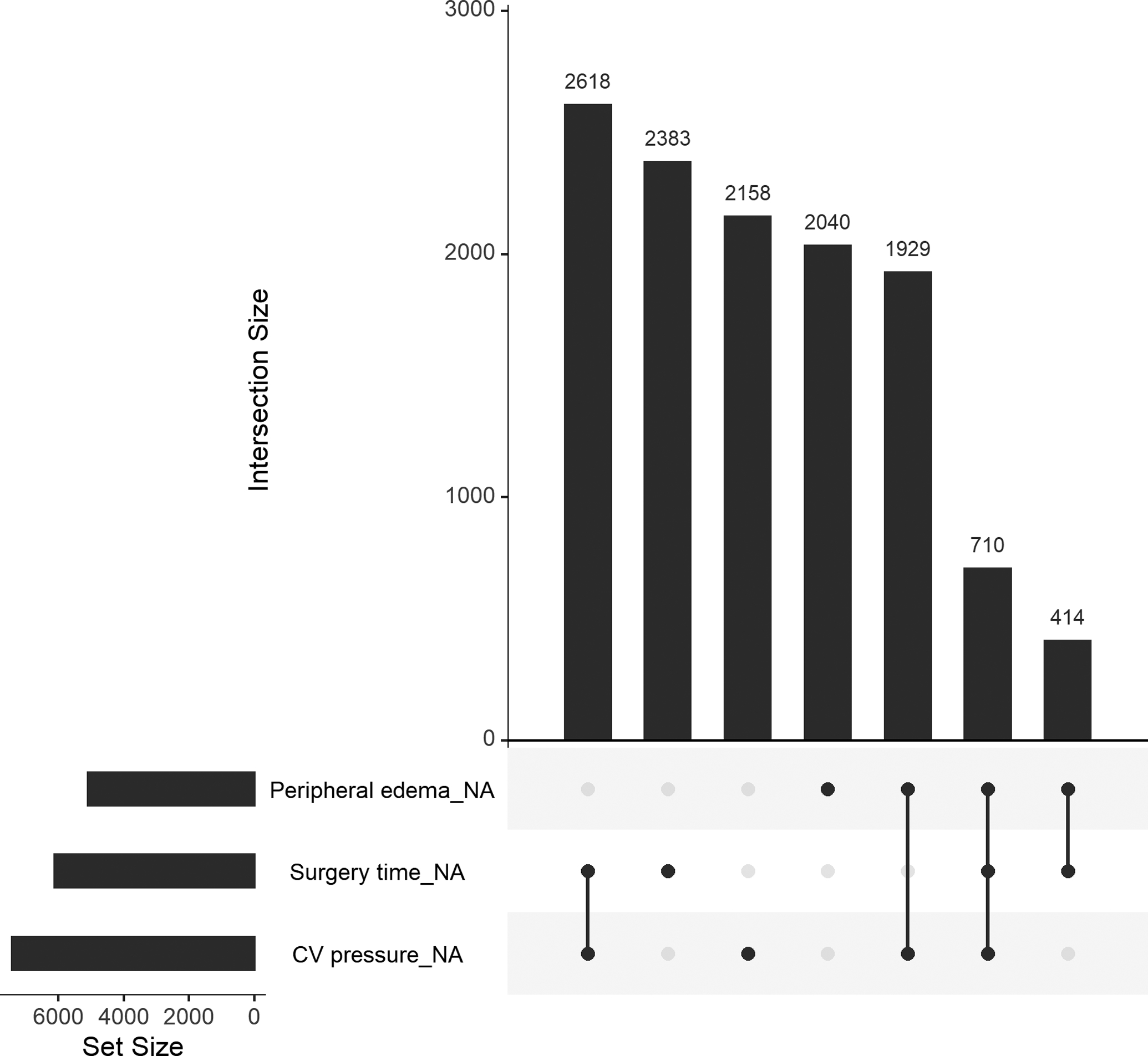
An upset plot showing three variables from the INTERMACS registry and all combinations of missing patterns. The bottom left plot shows the number of missing values for each variable, separately. The top right plot shows the number of missing values for each combination of the three variables. For example, there were 2,618 rows in the overall INTERMACS data where both CV pressure and surgery time were missing.

Imputation accuracy:

Single imputation strategies were more accurate than their counterparts using multiple imputation in 8 out of 10 comparisons of nominal scores and 10 out of 10 comparisons of numeric scores (Table 3). When an additional 15% of data were missing, single imputation KNN obtained the highest nominal accuracy (score: +0.02, 95% CI −0.05, 0.15) and single imputation with random forests obtained the highest numeric accuracy (score: +0.05, 95% CI 0.03, 0.08). When an additional 30% of data were missing, imputation to the mean obtained the highest numeric and nominal scores.

Table 3:

Accuracy of strategies to impute artificial missing data.

Imputation method	Nominal variables		Numeric variables
	Single imputation	Multiple imputation	Single imputation	Multiple imputation
+15% additional missing data
Imputation to the mean	0 (reference)	---	0 (reference)	---
Hot deck	−0.24 (−0.34, −0.16)	−0.25 (−0.37, −0.18)	−0.35 (−0.53, −0.29)	−0.42 (−0.54, −0.36)
K-nearest-neighbors	+0.02 (−0.05, 0.15)	−0.01 (−0.09, 0.11)	+0.01 (−0.01, 0.03)	−0.02 (−0.05, 0.00)
Predictive mean matching	−0.15 (−0.34, 0.00)	−0.15 (−0.35, 0.00)	−0.25 (−0.40, −0.20)	−0.26 (−0.35, −0.21)
Random forest	−0.15 (−0.26, −0.03)	−0.15 (−0.26, −0.03)	+0.05 (0.03, 0.08)	+0.02 (−0.01, 0.04)
Bayesian regression	−0.14 (−0.26, 0.01)	−0.14 (−0.27, 0.01)	−0.30 (−0.41, −0.23)	−0.30 (−0.41, −0.23)
+30% additional missing data
Imputation to the mean	0 (reference)	---	0 (reference)	---
Hot deck	−0.25 (−0.34, −0.18)	−0.26 (−0.36, −0.18)	−0.34 (−0.46, −0.30)	−0.40 (−0.53, −0.36)
K-nearest-neighbors	−0.04 (−0.09, 0.03)	−0.07 (−0.13, 0.00)	−0.02 (−0.03, −0.01)	−0.05 (−0.07, −0.04)
Predictive mean matching	−0.18 (−0.38, −0.04)	−0.18 (−0.37, −0.04)	−0.29 (−0.46, −0.24)	−0.29 (−0.40, −0.25)
Random forest	−0.18 (−0.28, −0.07)	−0.18 (−0.28, −0.08)	−0.01 (−0.03, 0.01)	−0.03 (−0.06, −0.01)
Bayesian regression	−0.17 (−0.29, −0.04)	−0.17 (−0.29, −0.05)	−0.31 (−0.43, −0.27)	−0.31 (−0.43, −0.27)

Table values are the median change in accuracy (25th, 75th percentile) relative to the accuracy of imputation to the mean. In general, multiple imputation strategies had lower accuracy than single imputation strategies, and few imputation strategies were more accurate than imputation to the mean.

Scaled Brier score

Mortality risk prediction:

When no additional data were amputed and imputation to the mean was applied before fitting risk prediction models, the median (25^th, 75^th percentile) scaled Brier score was 6.09 (5.71, 6.54) for Cox PH and 7.27 (6.83, 7.77) for boosting models (Table 4; top panel). Multiple imputation strategies universally obtained higher scaled Brier scores versus their single imputation counterparts. Multiple imputation using random forests provided the highest scaled Brier score compared to other strategies, leading to a median (25^th, 75^th percentile) increase in the scaled Brier score of 0.34 (0.12, 0.54) for Cox PH and 0.34 (0.14, 0.58) for boosting models. These performance increments improved when an additional 15% and 30% of data were amputed (Table 4; middle and bottom panel).

Table 4:

Median (25th, 75th percentile) change in scaled Brier score when different imputation strategies were applied to training and testing sets instead of imputation to the mean prior to developing a risk prediction model for mortality.

Imputation method	Proportional hazards		Gradient boosted decision trees
	Single imputation	Multiple imputation	Single imputation	Multiple imputation
No additional missing data
Imputation to the mean	6.09 (reference)	---	7.27 (reference)	---
Missingness as an attribute	---	---	+0.09 (−0.16, 0.31)	---
Hot deck	−0.25 (−0.47, 0.01)	+0.05 (−0.15, 0.24)	−0.24 (−0.46, 0.03)	+0.25 (0.08, 0.45)
K-nearest-neighbors	+0.09 (−0.06, 0.23)	+0.18 (0.04, 0.34)	−0.06 (−0.27, 0.18)	+0.28 (0.06, 0.46)
Predictive mean matching	−0.30 (−0.53, −0.03)	+0.15 (−0.01, 0.37)	−0.22 (−0.43, 0.14)	+0.34 (0.13, 0.54)
Random forest	+0.05 (−0.24, 0.33)	+0.34 (0.12, 0.54)	−0.08 (−0.32, 0.21)	+0.34 (0.14, 0.58)
Bayesian regression	−0.35 (−0.61, −0.10)	+0.07 (−0.10, 0.29)	−0.25 (−0.52, 0.05)	+0.29 (0.08, 0.52)
+15% additional missing data
Imputation to the mean	5.56 (reference)	---	6.72 (reference)	---
Missingness as an attribute	---	---	+0.52 (0.21, 0.77)	---
Hot deck	+0.10 (−0.22, 0.46)	+0.49 (0.21, 0.78)	+0.02 (−0.28, 0.33)	+0.58 (0.29, 0.92)
K-nearest-neighbors	+0.36 (0.10, 0.65)	+0.53 (0.25, 0.79)	+0.04 (−0.23, 0.36)	+0.42 (0.16, 0.68)
Predictive mean matching	+0.03 (−0.32, 0.41)	+0.54 (0.20, 0.90)	+0.21 (−0.25, 0.64)	+0.66 (0.32, 1.12)
Random forest	+0.39 (−0.05, 0.75)	+0.76 (0.37, 1.12)	+0.35 (0.01, 0.76)	+0.73 (0.41, 1.06)
Bayesian regression	+0.05 (−0.44, 0.44)	+0.49 (0.10, 0.85)	+0.19 (−0.21, 0.59)	+0.58 (0.29, 1.06)
+30% additional missing data
Imputation to the mean	4.79 (reference)	---	6.29 (reference)	---
Missingness as an attribute	---	---	+0.40 (0.11, 0.75)	---
Hot deck	+0.47 (0.03, 0.99)	+0.73 (0.22, 1.38)	+0.10 (−0.24, 0.44)	+0.51 (0.05, 0.99)
K-nearest-neighbors	+0.57 (0.23, 0.97)	+0.77 (0.47, 1.18)	−0.09 (−0.44, 0.23)	+0.36 (0.09, 0.67)
Predictive mean matching	+0.25 (−0.36, 0.82)	+0.71 (0.16, 1.36)	+0.09 (−0.33, 0.64)	+0.58 (0.06, 1.05)
Random forest	+0.62 (0.08, 1.22)	+1.04 (0.39, 1.83)	+0.39 (−0.19, 0.77)	+0.69 (0.27, 1.12)
Bayesian regression	+0.22 (−0.40, 0.82)	+0.68 (0.10, 1.28)	+0.10 (−0.44, 0.62)	+0.43 (−0.03, 0.93)

Table values show the scaled Brier score when the imputation method is imputation to the mean and the change in scaled Brier score relative to imputation to the mean for other imputation strategies. All table values are multiplied by 100 for ease of interpretation. Multiple imputation with random forests leads to the highest scaled Brier score for both models and when 0%, 15%, or 30% of additional data in the training and testing sets were set to missing.

Transplant risk prediction:

When no additional data were amputed and imputation to the mean was applied before fitting risk prediction models, the median (25^th, 75^th percentile) scaled Brier score was 9.35 (8.80, 9.71) for Cox PH and 9.00 (8.55, 9.41) for boosting models (Table 5; top panel). For Cox PH models, imputation to the mean provided the lowest scaled Brier score, and random forest imputation led to a median (25^th, 75^th percentile) increase of 0.13 (0.03, 0.29) versus imputation to the mean. For boosting models, surprisingly, imputation to the mean provided a higher scaled Brier score than all imputation methods except for multiple imputation using Bayesian regression. When an additional 15% and 30% of data were amputed, the performance increments corresponding to the use of multiple imputation increased for both Cox PH and boosting models (Table 5; middle and bottom panel).

Table 5:

Median (25th, 75th percentile) change in scaled Brier score when different imputation strategies were applied to training and testing sets instead of imputation to the mean prior to developing a risk prediction model for transplant.

Imputation method	Proportional hazards		Gradient boosted decision trees
	Single imputation	Multiple imputation	Single imputation	Multiple imputation
No additional missing data
Imputation to the mean	9.35 (reference)	---	9.00 (reference)	---
Missingness as an attribute	---	---	−0.07 (−0.28, 0.13)	---
Hot deck	+0.01 (−0.12, 0.15)	+0.06 (−0.04, 0.23)	−0.24 (−0.43, 0.04)	−0.01 (−0.20, 0.17)
K-nearest-neighbors	+0.06 (−0.04, 0.17)	+0.08 (0.00, 0.19)	−0.27 (−0.50, −0.05)	−0.05 (−0.20, 0.10)
Predictive mean matching	+0.04 (−0.12, 0.19)	+0.14 (0.02, 0.29)	−0.34 (−0.60, −0.10)	−0.06 (−0.23, 0.15)
Random forest	+0.03 (−0.10, 0.19)	+0.13 (0.03, 0.29)	−0.32 (−0.50, −0.07)	−0.05 (−0.21, 0.14)
Bayesian regression	+0.03 (−0.13, 0.16)	+0.10 (0.00, 0.26)	−0.32 (−0.58, −0.05)	+0.02 (−0.13, 0.25)
+15% additional missing data
Imputation to the mean	8.76 (reference)	---	8.01 (reference)	---
Missingness as an attribute	---	---	+0.50 (0.27, 0.78)	---
Hot deck	+0.25 (−0.04, 0.55)	+0.42 (0.20, 0.78)	−0.10 (−0.34, 0.23)	+0.21 (−0.02, 0.52)
K-nearest-neighbors	+0.46 (0.20, 0.73)	+0.54 (0.28, 0.79)	−0.10 (−0.41, 0.20)	+0.12 (−0.12, 0.38)
Predictive mean matching	+0.45 (0.10, 0.76)	+0.65 (0.34, 0.94)	−0.03 (−0.34, 0.21)	+0.25 (0.02, 0.62)
Random forest	+0.44 (0.12, 0.76)	+0.60 (0.32, 0.95)	−0.07 (−0.35, 0.26)	+0.16 (−0.09, 0.47)
Bayesian regression	+0.53 (0.21, 0.79)	+0.74 (0.37, 0.94)	−0.07 (−0.39, 0.24)	+0.24 (−0.09, 0.56)
+30% additional missing data
Imputation to the mean	7.96 (reference)	---	7.09 (reference)	---
Missingness as an attribute	---	---	+0.83 (0.55, 1.10)	---
Hot deck	+0.45 (−0.02, 0.90)	+0.60 (0.15, 1.11)	−0.01 (−0.34, 0.41)	+0.19 (−0.17, 0.65)
K-nearest-neighbors	+0.42 (0.00, 0.79)	+0.61 (0.18, 0.90)	−0.21 (−0.54, 0.19)	+0.09 (−0.22, 0.46)
Predictive mean matching	+0.70 (0.21, 1.21)	+0.90 (0.46, 1.46)	+0.09 (−0.32, 0.54)	+0.34 (−0.04, 0.85)
Random forest	+0.70 (0.14, 1.27)	+0.93 (0.49, 1.45)	−0.13 (−0.46, 0.43)	+0.25 (−0.12, 0.66)
Bayesian regression	+0.77 (0.32, 1.40)	+1.00 (0.44, 1.53)	0.00 (−0.45, 0.52)	+0.24 (−0.17, 0.80)

Table values show the scaled Brier score when the imputation method is imputation to the mean and the change in scaled Brier score relative to imputation to the mean for other imputation strategies. All table values are multiplied by 100 for ease of interpretation. While there was very little difference in scaled Brier score values when 0% of additional data were set to missing in the training and testing sets, missingness incorporated as an attribute, predictive mean matching, random forests, and Bayesian regression provided models with higher scaled Brier scores when 15% or 30% of additional missing data were amputed.

Discrimination and calibration

Mortality risk prediction:

Regardless of how much additional data were amputed, boosting models obtained higher median C-indices than PH models for prediction of 6-month mortality risk (Table 6). In addition, all models that used multiple imputation consistently obtained higher median C-indices compared to their counterparts using single imputation. When 0 and 15% additional data were amputed, median calibration error was lower for PH models compared to boosting models, but boosting models obtained lower median calibration error when 30% additional data were amputed (Table 7). Almost all imputation strategies provided lower median calibration error compared with imputation to the mean.

Table 6:

Median (25th, 75th percentile) change in concordance index when different imputation strategies were applied to training and testing sets instead of imputation to the mean prior to developing a risk prediction model for mortality.

Imputation method	Proportional hazards		Gradient boosted decision trees
	Single imputation	Multiple imputation	Single imputation	Multiple imputation
No additional missing data
Imputation to the mean	69.3 (reference)	---	70.7 (reference)	---
Missingness as an attribute	---	---	0.00 (−0.20, 0.19)	---
Hot deck	−0.20 (−0.44, 0.05)	+0.04 (−0.13, 0.27)	−0.19 (−0.36, 0.00)	+0.13 (−0.04, 0.28)
K-nearest-neighbors	+0.03 (−0.10, 0.23)	+0.14 (−0.02, 0.36)	−0.10 (−0.30, 0.13)	+0.14 (−0.03, 0.30)
Predictive mean matching	−0.34 (−0.56, −0.03)	+0.11 (−0.05, 0.37)	−0.21 (−0.44, 0.05)	+0.21 (0.06, 0.39)
Random forest	+0.04 (−0.24, 0.29)	+0.30 (0.08, 0.52)	−0.02 (−0.26, 0.18)	+0.24 (0.07, 0.41)
Bayesian regression	−0.39 (−0.69, −0.10)	+0.09 (−0.16, 0.28)	−0.21 (−0.44, −0.02)	+0.22 (0.06, 0.41)
+15% additional missing data
Imputation to the mean	69.2 (reference)	---	70.5 (reference)	---
Missingness as an attribute	---	---	+0.10 (−0.11, 0.31)	---
Hot deck	−0.18 (−0.52, 0.19)	+0.25 (−0.07, 0.58)	−0.23 (−0.50, 0.03)	+0.12 (−0.07, 0.32)
K-nearest-neighbors	+0.16 (−0.17, 0.42)	+0.30 (0.05, 0.56)	−0.16 (−0.33, 0.10)	+0.10 (−0.07, 0.31)
Predictive mean matching	−0.42 (−0.83, 0.02)	+0.24 (−0.07, 0.53)	−0.26 (−0.54, 0.00)	+0.26 (0.06, 0.43)
Random forest	−0.04 (−0.39, 0.26)	+0.41 (0.05, 0.64)	−0.08 (−0.29, 0.19)	+0.27 (0.04, 0.43)
Bayesian regression	−0.50 (−0.95, −0.06)	+0.20 (−0.11, 0.47)	−0.29 (−0.48, −0.03)	+0.23 (0.07, 0.43)
+30% additional missing data
Imputation to the mean	68.9 (reference)	---	70.2 (reference)	---
Missingness as an attribute	---	---	+0.12 (−0.08, 0.31)	---
Hot deck	−0.15 (−0.52, 0.30)	+0.12 (−0.23, 0.51)	−0.22 (−0.47, 0.02)	+0.10 (−0.17, 0.32)
K-nearest-neighbors	+0.17 (−0.11, 0.49)	+0.33 (0.09, 0.65)	−0.08 (−0.27, 0.16)	+0.19 (−0.01, 0.38)
Predictive mean matching	−0.75 (−1.15, −0.34)	+0.06 (−0.29, 0.52)	−0.36 (−0.67, −0.04)	+0.27 (0.04, 0.48)
Random forest	−0.29 (−0.80, 0.23)	+0.26 (−0.10, 0.64)	−0.16 (−0.47, 0.11)	+0.29 (0.07, 0.52)
Bayesian regression	−0.75 (−1.28, −0.22)	+0.12 (−0.29, 0.48)	−0.36 (−0.70, −0.07)	+0.19 (−0.01, 0.44)

Table values show the concordance index when the imputation method is imputation to the mean and the change in concordance index relative to imputation to the mean for other imputation strategies. All table values are multiplied by 100 for ease of interpretation. Multiple imputation with random forests led to the highest concordance index for boosting models when 0%, 15%, or 30% of additional data in the training and testing sets were set to missing. For proportional hazards models, multiple imputation with nearest neighbors or random forests was the most effective strategy.

Table 7:

Median (25th, 75th percentile) change in calibration error when different imputation strategies were applied to training and testing sets instead of imputation to the mean prior to developing a risk prediction model for mortality.

Imputation method	Proportional hazards		Gradient boosted decision trees
	Single imputation	Multiple imputation	Single imputation	Multiple imputation
No additional missing data
Imputation to the mean	2.41 (reference)	---	3.29 (reference)	---
Missingness as an attribute	---	---	−0.09 (−1.07, 0.65)	---
Hot deck	−0.04 (−0.68, 0.58)	−0.45 (−1.25, 0.25)	−0.13 (−1.12, 0.65)	−0.90 (−1.98, 0.01)
K-nearest-neighbors	+0.04 (−0.59, 0.65)	−0.29 (−0.80, 0.39)	−0.30 (−1.14, 0.61)	−0.75 (−1.59, 0.14)
Predictive mean matching	−0.18 (−0.69, 0.47)	−0.69 (−1.36, −0.03)	−0.11 (−1.27, 0.89)	−1.02 (−2.08, −0.12)
Random forest	−0.07 (−0.58, 0.65)	−0.46 (−1.10, 0.17)	−0.56 (−1.38, 0.46)	−1.10 (−2.08, −0.14)
Bayesian regression	−0.08 (−0.75, 0.53)	−0.57 (−1.43, 0.02)	−0.26 (−1.08, 0.57)	−0.85 (−1.91, 0.12)
+15% additional missing data
Imputation to the mean	5.75 (reference)	---	6.28 (reference)	---
Missingness as an attribute	---	---	−2.83 (−4.81, −0.83)	---
Hot deck	−2.16 (−4.31, −1.08)	−3.92 (−6.23, −1.72)	−1.66 (−3.82, −0.34)	−3.44 (−5.97, −1.48)
K-nearest-neighbors	−2.01 (−3.51, −0.66)	−2.48 (−4.08, −1.14)	−0.61 (−2.28, 0.84)	−2.04 (−3.32, −0.63)
Predictive mean matching	−3.83 (−6.40, −1.87)	−3.76 (−6.66, −1.04)	−3.52 (−6.43, −1.67)	−3.50 (−7.09, −1.00)
Random forest	−3.80 (−5.75, −2.07)	−4.35 (−6.60, −1.53)	−3.74 (−6.34, −1.34)	−3.92 (−6.29, −1.50)
Bayesian regression	−3.76 (−6.45, −1.81)	−3.80 (−6.61, −1.04)	−3.79 (−6.80, −1.39)	−3.27 (−6.40, −0.46)
+30% additional missing data
Imputation to the mean	9.48 (reference)	---	7.02 (reference)	---
Missingness as an attribute	---	---	−1.61 (−5.29, 0.68)	---
Hot deck	−4.95 (−9.18, −2.49)	−6.69 (−12.8, −1.56)	−2.48 (−5.46, −0.31)	−2.48 (−7.18, 0.58)
K-nearest-neighbors	−3.47 (−6.42, −1.53)	−4.49 (−7.49, −2.39)	+0.73 (−1.56, 3.27)	−1.47 (−3.59, 0.59)
Predictive mean matching	−7.33 (−13.0, −2.61)	−6.09 (−12.3, −0.22)	−2.58 (−7.90, 0.10)	−1.30 (−6.86, 2.29)
Random forest	−7.81 (−13.1, −3.63)	−7.39 (−13.4, −2.37)	−3.53 (−7.87, −0.29)	−2.58 (−7.27, 0.44)
Bayesian regression	−7.27 (−13.2, −2.44)	−5.91 (−12.8, −0.47)	−3.00 (−7.60, 0.97)	−0.54 (−6.60, 3.08)

Table values show the calibration error when the imputation method is imputation to the mean and the change in calibration error relative to imputation to the mean for other imputation strategies. All table values are multiplied by 100 for ease of interpretation. As more data in the training and testing sets were set to missing, single and multiple imputation with random forests emerged as the strategies with the lowest calibration error.

Transplant risk prediction:

For all amounts of additional data amputed, PH models obtained higher median C-indices than boosting models for prediction of 6-month transplant risk (Table 8). Similar to mortality risk prediction, multiple imputation strategies generally provided higher C-indices than their counterparts using single imputation strategy. For boosting models, MIA provided higher C-indices compared to all other single imputation strategies and had similar or superior performance compared to several multiple imputation strategies. Differences in calibration error were minor when no additional missing data were amputed (Table 9). When an additional 30% of data were amputed, boosting models using MIA obtained lower calibration error than any other strategy.

Table 8:

Median (25th, 75th percentile) change in concordance index when different imputation strategies were applied to training and testing sets instead of imputation to the mean prior to developing a risk prediction model for transplant.

Imputation method	Proportional hazards		Gradient boosted decision trees
	Single imputation	Multiple imputation	Single imputation	Multiple imputation
No additional missing data
Imputation to the mean	79.4 (reference)	---	79.2 (reference)	---
Missingness as an attribute	---	---	−0.03 (−0.22, 0.14)	---
Hot deck	+0.01 (−0.12, 0.17)	+0.07 (−0.05, 0.23)	−0.24 (−0.40, −0.02)	−0.04 (−0.20, 0.15)
K-nearest-neighbors	+0.08 (−0.02, 0.16)	+0.08 (0.01, 0.17)	−0.21 (−0.40, −0.04)	−0.04 (−0.18, 0.10)
Predictive mean matching	+0.03 (−0.11, 0.16)	+0.13 (0.01, 0.24)	−0.34 (−0.57, −0.12)	−0.06 (−0.19, 0.16)
Random forest	+0.03 (−0.09, 0.17)	+0.15 (0.06, 0.24)	−0.26 (−0.46, −0.08)	−0.02 (−0.16, 0.14)
Bayesian regression	+0.01 (−0.15, 0.16)	+0.10 (0.01, 0.22)	−0.32 (−0.54, −0.10)	+0.02 (−0.13, 0.22)
+15% additional missing data
Imputation to the mean	78.9 (reference)	---	78.4 (reference)	---
Missingness as an attribute	---	---	+0.47 (0.26, 0.71)	---
Hot deck	+0.24 (0.04, 0.51)	+0.47 (0.26, 0.76)	−0.13 (−0.40, 0.22)	+0.29 (0.07, 0.58)
K-nearest-neighbors	+0.36 (0.21, 0.54)	+0.46 (0.29, 0.62)	−0.13 (−0.39, 0.17)	+0.17 (−0.06, 0.39)
Predictive mean matching	+0.32 (0.11, 0.58)	+0.56 (0.37, 0.82)	−0.12 (−0.38, 0.25)	+0.32 (0.14, 0.61)
Random forest	+0.32 (0.13, 0.64)	+0.59 (0.36, 0.82)	−0.11 (−0.40, 0.24)	+0.22 (−0.03, 0.51)
Bayesian regression	+0.39 (0.17, 0.63)	+0.60 (0.40, 0.83)	−0.15 (−0.46, 0.27)	+0.27 (−0.01, 0.64)
+30% additional missing data
Imputation to the mean	78.4 (reference)	---	77.4 (reference)	---
Missingness as an attribute	---	---	+0.91 (0.52, 1.24)	---
Hot deck	+0.34 (−0.03, 0.72)	+0.74 (0.48, 1.11)	−0.19 (−0.53, 0.34)	+0.55 (0.19, 0.86)
K-nearest-neighbors	+0.28 (−0.02, 0.47)	+0.43 (0.21, 0.66)	−0.32 (−0.78, −0.04)	−0.01 (−0.33, 0.31)
Predictive mean matching	+0.62 (0.29, 0.98)	+1.02 (0.74, 1.34)	+0.03 (−0.31, 0.44)	+0.65 (0.29, 0.95)
Random forest	+0.59 (0.22, 1.00)	+1.04 (0.76, 1.30)	−0.21 (−0.58, 0.15)	+0.36 (0.01, 0.68)
Bayesian regression	+0.81 (0.41, 1.08)	+1.10 (0.80, 1.39)	−0.04 (−0.54, 0.37)	+0.47 (0.10, 0.91)

Table values show the concordance index when the imputation method is imputation to the mean and the change in concordance index relative to imputation to the mean for other imputation strategies. All table values are multiplied by 100 for ease of interpretation. While there was little difference in concordance index when 0% of additional data were set to missing in the training and testing sets, missingness incorporated as an attribute, predictive mean matching, random forests, and Bayesian regression provided models with higher concordance indices when 15% or 30% of additional missing data were amputed.

Table 9:

Median (25th, 75th percentile) change in calibration error when different imputation strategies were applied to training and testing sets instead of imputation to the mean prior to developing a risk prediction model for transplant.

Imputation method	Proportional hazards		Gradient boosted decision trees
	Single imputation	Multiple imputation	Single imputation	Multiple imputation
No additional missing data
Imputation to the mean	1.36 (reference)	---	1.79 (reference)	---
Missingness as an attribute	---	---	+0.01 (−0.53, 0.54)	---
Hot deck	−0.01 (−0.37, 0.29)	0.00 (−0.39, 0.26)	+0.11 (−0.56, 0.68)	−0.07 (−0.67, 0.67)
K-nearest-neighbors	+0.00 (−0.25, 0.24)	−0.02 (−0.25, 0.21)	+0.09 (−0.40, 0.61)	−0.03 (−0.52, 0.67)
Predictive mean matching	−0.04 (−0.34, 0.32)	−0.08 (−0.41, 0.26)	+0.09 (−0.49, 0.63)	−0.04 (−0.63, 0.70)
Random forest	−0.06 (−0.39, 0.29)	−0.06 (−0.35, 0.29)	−0.02 (−0.49, 0.63)	+0.02 (−0.54, 0.56)
Bayesian regression	−0.01 (−0.40, 0.27)	−0.13 (−0.38, 0.18)	+0.12 (−0.46, 0.78)	+0.24 (−0.46, 1.04)
+15% additional missing data
Imputation to the mean	2.48 (reference)	---	2.51 (reference)	---
Missingness as an attribute	---	---	−0.50 (−1.38, 0.16)	---
Hot deck	−0.76 (−1.95, 0.21)	−0.51 (−2.14, 0.89)	−0.01 (−1.00, 0.66)	+0.69 (−0.47, 1.97)
K-nearest-neighbors	−0.82 (−2.01, 0.21)	−0.78 (−1.96, 0.26)	+0.20 (−0.59, 1.01)	+0.23 (−0.73, 1.02)
Predictive mean matching	−1.01 (−2.15, 0.27)	−0.46 (−2.16, 0.94)	+0.15 (−0.91, 1.02)	+0.72 (−0.81, 1.87)
Random forest	−0.80 (−2.32, 0.51)	−0.59 (−2.03, 0.81)	−0.10 (−1.15, 0.66)	+0.42 (−0.93, 1.34)
Bayesian regression	−0.94 (−2.32, 0.58)	−0.64 (−2.04, 0.89)	+0.19 (−0.76, 1.16)	+0.99 (−0.50, 2.27)
+30% additional missing data
Imputation to the mean	4.98 (reference)	---	3.99 (reference)	---
Missingness as an attribute	---	---	−1.52 (−2.62, −0.35)	---
Hot deck	−2.17 (−4.65, 0.10)	−0.49 (−3.74, 2.34)	−0.53 (−2.79, 1.05)	+1.89 (−0.93, 4.76)
K-nearest-neighbors	−1.88 (−3.34, −0.22)	−1.88 (−3.70, −0.14)	−0.41 (−1.72, 0.68)	−0.54 (−2.26, 0.88)
Predictive mean matching	−1.30 (−4.52, 1.28)	+0.04 (−3.48, 2.70)	−0.05 (−2.54, 2.53)	+1.36 (−1.26, 4.01)
Random forest	−1.80 (−4.34, 0.79)	−0.58 (−3.95, 2.18)	−0.55 (−2.64, 1.53)	+0.33 (−2.27, 2.77)
Bayesian regression	−1.34 (−4.22, 1.59)	−0.23 (−3.15, 2.61)	−0.16 (−2.47, 1.94)	+0.89 (−1.89, 3.67)

Table values show the calibration error when the imputation method is imputation to the mean and the change in calibration error relative to imputation to the mean for other imputation strategies. All table values are multiplied by 100 for ease of interpretation. As more data in the training and testing sets were set to missing, single and multiple imputation with nearest neighbors emerged as the optimal strategy for proportional hazards models while missingness incorporated as an attributed emerged an the optimal strategy for boosting models.

Bayesian analysis of model performance

Adjusting for the amount of additional missing data amputed and the outcome variable, the posterior probability that an imputation strategy would improve the scaled Brier score of a downstream model relative to imputation to the mean was maximized by using multiple imputation with random forests (probability of improvement: >0.999; Figure 2). Similarly, multiple imputation using random forests was estimated to have the highest posterior probability of improving the C-index in comparison to using imputation to the mean (probability of improvement: >0.999; Figure 3). However, the estimated posterior probability of a reduction in calibration was >0.999 when using either single or multiple imputation with random forests compared with imputation to the mean (Figure 4). Although imputation using random forest was estimated to be the best overall option, there was moderate to strong evidence that MIA and each multiple imputation strategy we applied would improve prognostic accuracy of downstream models compared with imputation to the mean.

Figure 2:

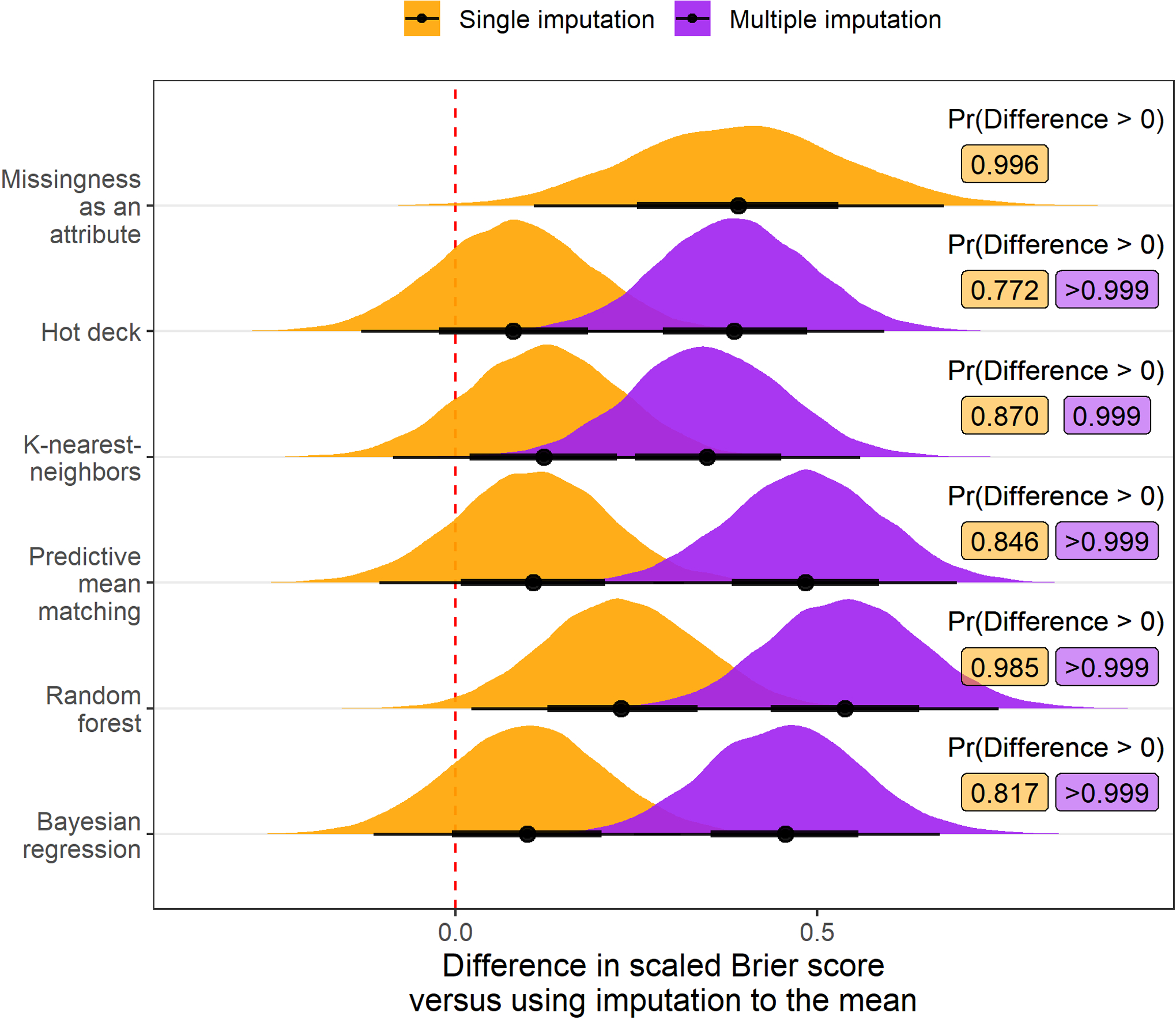
Posterior distribution of differences in scaled Brier score values (multiplied by 100) relative to imputation to the mean when different imputation strategies are applied before fitting a risk prediction model. Results are aggregated over scenarios where the outcome is mortality and transplant and the amount of additional missing data is 0%, 15%, or 30%. Posterior probability that the difference in scaled Brier score exceeds 0, indicating an improvement in overall model accuracy, is printed to the right of each distribution. Each multiple imputation strategy and single imputation with missingness incorporated as an attribute had over 90% posterior predicted probability of increasing the scaled Brier score versus using imputation to the mean.

Figure 3:

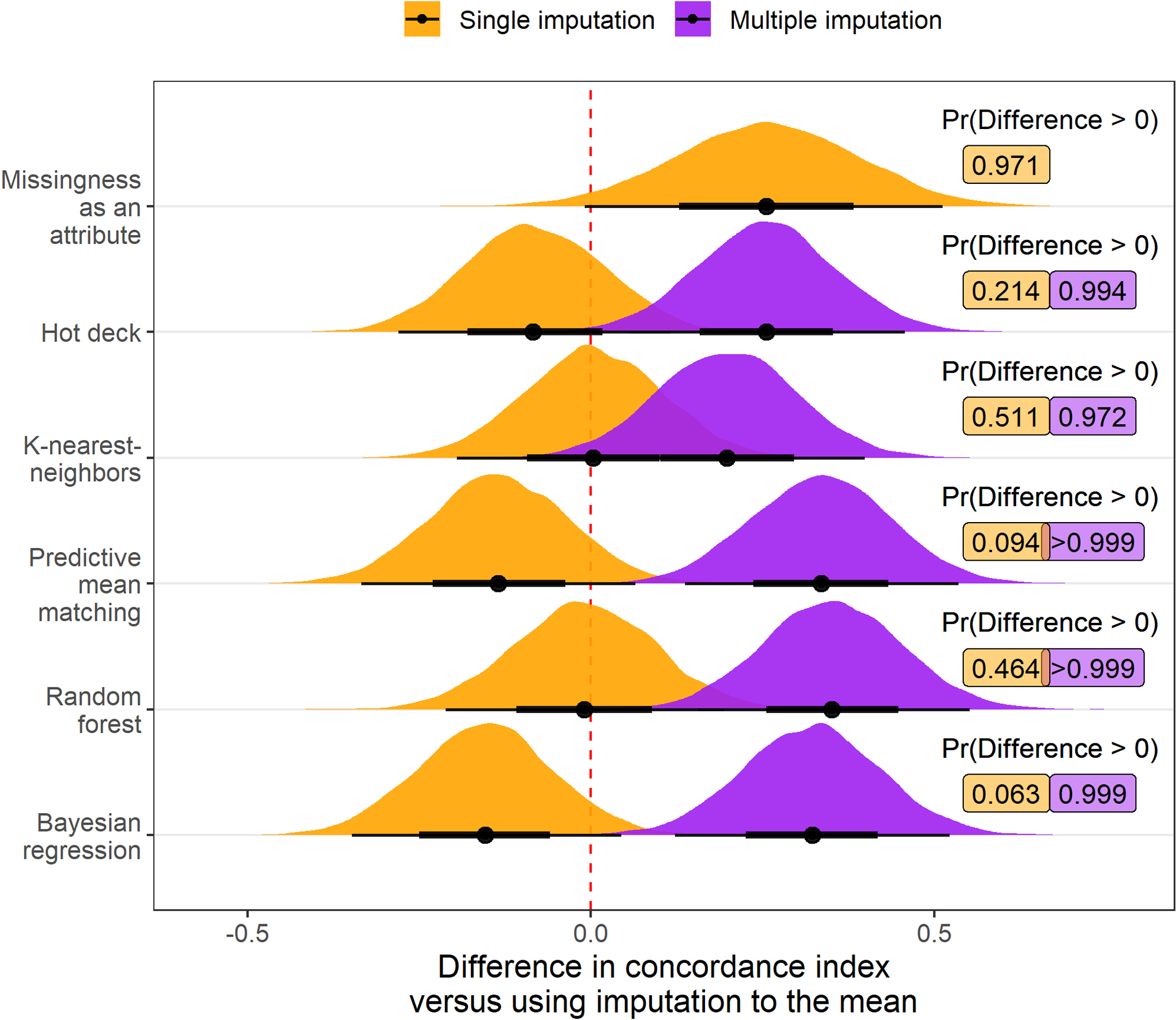
Posterior distribution of differences in concordance index values (multiplied by 100) relative to imputation to the mean when different imputation strategies are applied before fitting a risk prediction model. Results are aggregated over scenarios where the outcome is mortality and transplant and the amount of additional missing data is 0%, 15%, or 30%. Posterior probability that the difference in concordance index exceeds 0, indicating an improvement in model discrimination, is printed to the right of each distribution. Multiple imputation with predictive mean matching, random forests, and Bayesian regression each had over 90% posterior predicted probability of increasing the concordance index versus using imputation to the mean.

Figure 4:

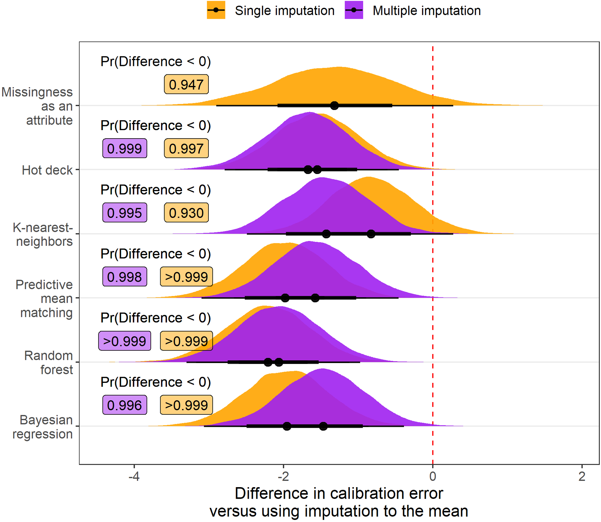
Posterior distribution of differences in calibration error values (multiplied by 100) relative to imputation to the mean when different imputation strategies are applied before fitting a risk prediction model. Results are aggregated over scenarios where the outcome is mortality and transplant and the amount of additional missing data is 0%, 15%, or 30%. Posterior probability that the difference in calibration error is less than 0, indicating an improvement in model calibration, is printed to the right of each distribution. Every imputation strategy evaluated had over 90% posterior predicted probability of improving model calibration versus using imputation to the mean.

Summary

Multiple imputation with random forests emerged as a robust strategy to impute missing values, leading to superior model concordance and scaled Brier score compared to other imputation techniques. In addition to random forests, PMM and Bayesian regression also improved model discrimination and scaled Brier score relative to imputation to the mean, and these improvements were enhanced by the use of multiple imputation versus single imputation. Based on the computational budget of a future analysis, data from the current analysis support the use of any of these three imputation techniques. Despite its relatively high imputation accuracy, KNN imputation was less beneficial for the prognostic accuracy of downstream models compared to random forests, PMM, and Bayesian regression. There was little difference across imputation techniques in terms of calibration error. A summary of the benefits, drawbacks, and recommendation for each imputation technique studied in the current analysis is presented in Table 10

Table 10:

Summary of the missing data strategies studied in the current analysis.

Imputation strategy	Description	Benefits	Drawbacks	Recommendation
Imputation to the mean	Imputes missing values with mean for continuous and mode for categorical variables	Computationally efficient Straightforward to implement in testing data High imputation accuracy	Lower prognostic accuracy for downstream models	Useful when the proportion of missing values is low or when imputation accuracy is higher priority than prognostic accuracy of downstream models.
Missingness as an attribute	Treats missing status as a category for predictor variables	Computationally efficient Highest prognostic accuracy of downstream models among single imputation techniques	Difficult to implement for continuous variables in traditional statistical models	Useful when the modeling algorithm involves decision trees and computational efficiency is a high priority.
Hot deck	Uses observations from similar cases based on sorting	More computationally efficient than other imputation techniques Less restrictive assumptions since models are not used	Low imputation accuracy and prognostic accuracy of downstream models when single imputation is applied	Useful when multiple imputation is feasible
K-nearest-neighbors	Uses observations from similar cases based on Gower’s distance	Flexible Most accurate imputed values when single imputation is applied	Computationally inefficient and scales poorly to larger datasets	Useful in a broad range of scenarios if computationally feasible
Predictive mean matching	Uses observations from similar cases based on predicted values from a model	Flexible Intuitive	Models may become computationally intractable with larger proportions of missing data or collinearity in predictors	Useful when multiple imputation is feasible
Random forest	Applies random forests to impute missing values, iterating until error estimates stabilize	Accurate imputed values for numeric variables when single imputation is applied Most accurate prognostic accuracy of downstream models when multiple imputation is applied	Very high computational overhead and requires large amounts of memory to store random forest models for imputation of new data	Useful in a broad range of scenarios for single or multiple imputation, if computationally feasible
Bayesian regression	Draws imputed values from posterior distributions, accounting for model uncertainty	Computationally efficient High prognostic accuracy of downstream models when multiple imputation is applied	May require assumptions for Bayesian modeling	Useful when multiple imputation is feasible

DISCUSSION

In this article, we leveraged INTERMACS registry data to evaluate how the use of different imputation strategies prior to fitting a risk prediction model would impact the external prognostic accuracy of the model. External prognostic accuracy was measured at 6 months after receiving MCS, and the primary measure of accuracy was the scaled Brier score. We evaluated the performance of 12 imputation strategies in a broad range of settings by varying (1) the amount of additional missing data amputed prior to performing imputation, (2) the type of risk prediction model applied after imputation, and (3) the outcome variable for the risk prediction model. Our resampling experiment indicated that conducting multiple imputation has a high likelihood of increasing the downstream scaled Brier score and C-index of risk prediction models compared with imputation to the mean. Additionally, multiple imputation with random forests emerged as the imputation strategy that maximized the probability of developing a more prognostic model compared with imputation to the mean.

In previous studies involving the INTERMACS data registry, imputation to the mean has been applied prior to developing a mortality risk prediction model.^7–12 An interesting recent study indicates that imputation to the mean can provide an asymptotically consistent prediction model, given the prediction model is flexible and non-linear.²⁰ However, theoretical results for finite samples have not yet been established. Our results provide relevant data for the finite sample case, suggesting that using imputation strategies considered in the current study instead of imputation to the mean can improve the prognostic accuracy of downstream models, particularly if multiple imputation is applied. In scenarios where few variables have missing values and the proportion of missing values is low, imputation to the mean is likely to be just as good as other strategies with more flexibility. As the amount and complexity of missingness increases, using multiple imputation and more flexible imputation models appears to offer a small increment in the prognostic accuracy of downstream models.

Previous research has also established evidence in favor of applying multiple imputation to improve the prognostic value of risk prediction models. For example, Hassan and Atiya demonstrated superior downstream prediction using an ensemble multiple imputation method on synthetic data with continuous outcomes.⁶⁴ Similarly, Nanni et. al demonstrated superior performance in downstream prediction when missing values were imputed using their proposed ensemble multiple imputation method.⁶⁵ Notably, the authors artificially induced missing values in these studies and the largest real dataset that was evaluated contained less than 700 observations. An article by Jerez et. al evaluated missing data strategies based on the downstream task of fitting a neural network and predicting early breast cancer relapse.¹⁹ The authors found that KNN imputation led to risk prediction models with the highest discrimination and lowest calibration error. Results from the current study are consistent with these previous findings but also extend their results by providing evidence from a larger source of data (i.e. INTERMACS) and dealing with ‘real-world’ missing values.

Others have previously evaluated imputation techniques based on the accuracy with which these techniques impute missing values in the training data.^66–68 While it is intuitive to hypothesize that more accurate imputation will provide more prognostic downstream models, our results do not support this supposition. For example, when an additional 30% of missing data were amputed, none of the missing data strategies we implemented obtained higher accuracy than imputation to the mean and multiple imputation strategies obtained particularly low accuracy. However, all of the multiple imputation strategies improved the prognostic accuracy of downstream models relative to imputation to the mean when an additional 30% of data were amputed prior to imputation of missing values. This result is likely explained by the bias variance tradeoff. In particular, single imputation techniques may lead to prediction models with lower bias but higher variance than multiple imputation techniques.

Strengths and limitations:

The current analysis has a number of strengths. We leveraged the INTERMACS data registry, comprising one of the largest cohorts of patients who received MCS. We applied a well known resampling method to internally validate modeling algorithms for risk prediction. We also made our analysis R code available in a public repository (https://github.com/bcjaeger/INTERMACS-missing-data). Last, the approach presented in this paper provides a general framework that can be applied in other studies where missing data are imputed prior to fitting a risk prediction model. The current analysis should also be interpreted in the context of known limitations. We considered a small subset of existing strategies to impute missing data, and other strategies may have provided stronger improvements compared with imputation to the mean. Our results are limited in scope to mortality and transplant outcomes, which are difficult to predict using data collected prior to the surgery where mechanical circulatory support is applied. Future analyses should investigate whether greater improvements are obtained based on the choice of imputation strategy for outcomes with greater correlation to the predictors that are being imputed. Also, it was not feasible to use only the training data to impute missing values in the testing data due to a lack of available software. Although the miceRanger R package allows imputation of new data using existing models, few software packages for imputation allow users to implement multiple imputation with this protocol. Future analyses should introduce more flexible software and hands-on tutorials so that investigators can optimize imputation of missing data.

Conclusion:

Selecting an optimal strategy to impute missing values such as random forests can impact the prognostic accuracy of downstream risk prediction models. In the current analysis, conducting multiple imputation using random forests emerged as an optimal strategy to impute missing values in the INTERMACS data. This investigation can directly inform future analyses of INTERMACS data and provide evidence quantifying the benefit of imputing missing data with sound methodology.

REFERENCES

- 1.Benjamin EJ, Blaha MJ, Chiuve SE, Cushman M, Das SR, Deo R, et al. Heart disease and stroke statistics-2017 update: A report from the american heart association. Circulation 2017;135:e146–e603. [DOI] [PMC free article] [PubMed] [Google Scholar]
- 2.Health Statistics NC for. Health, united states, 2016, with chartbook on long-term trends in health. Government Printing Office; 2017. [PubMed] [Google Scholar]
- 3.Patel CB, Cowger JA, Zuckermann A. A contemporary review of mechanical circulatory support. The Journal of Heart and Lung Transplantation 2014;33:667–674. [DOI] [PubMed] [Google Scholar]
- 4.Slaughter MS, Rogers JG, Milano CA, Russell SD, Conte JV, Feldman D, et al. Advanced heart failure treated with continuous-flow left ventricular assist device. New England Journal of Medicine 2009;361:2241–2251. [DOI] [PubMed] [Google Scholar]
- 5.Miller LW. Left ventricular assist devices are underutilized. Circulation 2011;123:1552–1558. [DOI] [PubMed] [Google Scholar]
- 6.Stewart GC, Stevenson LW. Keeping left ventricular assist device acceleration on track. Circulation 2011;123:1559–1568. [DOI] [PubMed] [Google Scholar]
- 7.Hsich EM, Naftel DC, Myers SL, Gorodeski EZ, Grady KL, Schmuhl D, et al. Should women receive left ventricular assist device support? Findings from INTERMACS. Circulation: Heart Failure 2012;5:234–240. [DOI] [PMC free article] [PubMed] [Google Scholar]
- 8.Cotts WG, McGee EC Jr, Myers SL, Naftel DC, Young JB, Kirklin JK, et al. Predictors of hospital length of stay after implantation of a left ventricular assist device: An analysis of the INTERMACS registry. The Journal of Heart and Lung Transplantation 2014;33:682–688. [DOI] [PMC free article] [PubMed] [Google Scholar]
- 9.Eckman P, Rosenbaum A, Vongooru H, Basraon J, John R, Levy W, et al. Survival of INTERMACS profile 4–6 patients after left ventricular assist device implant is improved compared to seattle heart failure model estimated survival. Journal of Cardiac Failure 2011;17:S38–S39. [Google Scholar]
- 10.Kirklin JK, Pagani FD, Kormos RL, Stevenson LW, Blume ED, Myers SL, et al. Eighth annual INTERMACS report: Special focus on framing the impact of adverse events. The Journal of Heart and Lung Transplantation 2017;36:1080–1086. doi:https://www.ncbi.nlm.nih.gov/pubmed/28942782. [DOI] [PubMed] [Google Scholar]
- 11.Kormos RL, Cowger J, Pagani FD, Teuteberg JJ, Goldstein DJ, Jacobs JP, et al. The society of thoracic surgeons INTERMACS database annual report: Evolving indications, outcomes, and scientific partnerships. The Journal of Heart and Lung Transplantation 2019;38:114–126. [DOI] [PubMed] [Google Scholar]
- 12.Adamo L, Tang Y, Nassif ME, Novak E, Jones PG, LaRue S, et al. The HeartMate risk score identifies patients with similar mortality risk across all INTERMACS profiles in a large multicenter analysis. JACC: Heart Failure 2016;4:950–958. doi: 10.1016/j.jchf.2016.07.014. [DOI] [PubMed] [Google Scholar]
- 13.Rubin DB. Multiple imputation for nonresponse in surveys. vol. 81. John Wiley & Sons; 2004. [Google Scholar]
- 14.Van Buuren S Flexible imputation of missing data. Chapman; Hall/CRC; 2018. doi: 10.1201/b11826. [DOI] [Google Scholar]
- 15.Sterne JA, White IR, Carlin JB, Spratt M, Royston P, Kenward MG, et al. Multiple imputation for missing data in epidemiological and clinical research: Potential and pitfalls. Bmj 2009;338. [DOI] [PMC free article] [PubMed] [Google Scholar]
- 16.van Ginkel JR, Linting M, Rippe RC, van der Voort A. Rebutting existing misconceptions about multiple imputation as a method for handling missing data. Journal of Personality Assessment 2020;102:297–308. [DOI] [PubMed] [Google Scholar]
- 17.Hastie T, Tibshirani R, Friedman J. The elements of statistical learning: Data mining, inference, and prediction. Springer Science & Business Media; 2009. [Google Scholar]
- 18.Kuhn M, Johnson K. Feature engineering and selection: A practical approach for predictive models. CRC Press; 2019. [Google Scholar]
- 19.Jerez JM, Molina I, García-Laencina PJ, Alba E, Ribelles N, Martín M, et al. Missing data imputation using statistical and machine learning methods in a real breast cancer problem. Artificial Intelligence in Medicine 2010;50:105–115. [DOI] [PubMed] [Google Scholar]
- 20.Josse J, Prost N, Scornet E, Varoquaux G. On the consistency of supervised learning with missing values. arXiv Preprint arXiv:1902069312019.
- 21.Thomas SS, Nahumi N, Han J, Lippel M, Colombo P, Yuzefpolskaya M, et al. Pre-operative mortality risk assessment in patients with continuous-flow left ventricular assist devices: Application of the HeartMate II risk score. The Journal of Heart and Lung Transplantation 2014;33:675–681. [DOI] [PubMed] [Google Scholar]
- 22.Azur MJ, Stuart EA, Frangakis C, Leaf PJ. Multiple imputation by chained equations: What is it and how does it work? International Journal of Methods in Psychiatric Research 2011;20:40–49. doi: 10.1002/mpr.329. [DOI] [PMC free article] [PubMed] [Google Scholar]
- 23.Van Buuren S, Brand JP, Groothuis-Oudshoorn CG, Rubin DB. Fully conditional specification in multivariate imputation. Journal of Statistical Computation and Simulation 2006;76:1049–1064. doi: 10.1080/10629360600810434. [DOI] [Google Scholar]
- 24.Landerman LR, Land KC, Pieper CF. An empirical evaluation of the predictive mean matching method for imputing missing values. Sociological Methods & Research 1997;26:3–33. doi: 10.1177/0049124197026001001. [DOI] [Google Scholar]
- 25.Chen J, Shao J. Nearest neighbor imputation for survey data. Journal of Official Statistics 2000;16:113. [Google Scholar]
- 26.Gower JC. A general coefficient of similarity and some of its properties. Biometrics 1971;27:857–871. [Google Scholar]
- 27.Andridge RR, Little RJ. A review of hot deck imputation for survey non-response. International Statistical Review 2010;78:40–64. doi: 10.1111/j.1751-5823.2010.00103.x. [DOI] [PMC free article] [PubMed] [Google Scholar]
- 28.Breiman L Random forests. Machine Learning 2001;45:5–32. doi: 10.1023/A:1010933404324. [DOI] [Google Scholar]
- 29.Hothorn T, Buehlmann P, Dudoit S, Molinaro A, Van Der Laan M. Survival ensembles. Biostatistics 2006;7:355–373. doi: 10.1093/biostatistics/kxj011. [DOI] [PubMed] [Google Scholar]
- 30.Strobl C, Boulesteix A-L, Zeileis A, Hothorn T. Bias in random forest variable importance measures: Illustrations, sources and a solution. BMC Bioinformatics 2007;8. [DOI] [PMC free article] [PubMed] [Google Scholar]
- 31.Strobl C, Boulesteix A-L, Kneib T, Augustin T, Zeileis A. Conditional variable importance for random forests. BMC Bioinformatics 2008;9. [DOI] [PMC free article] [PubMed] [Google Scholar]
- 32.Ishwaran H, Kogalur UB, Blackstone EH, Lauer MS, et al. Random survival forests. The Annals of Applied Statistics 2008;2:841–860. [Google Scholar]
- 33.Jaeger BC, Long DL, Long DM, Sims M, Szychowski JM, Min Y-I, et al. Oblique random survival forests. The Annals of Applied Statistics 2019;13:1847–1883. [DOI] [PMC free article] [PubMed] [Google Scholar]
- 34.Twala B An empirical comparison of techniques for handling incomplete data using decision trees. Applied Artificial Intelligence 2009;23:373–405. [Google Scholar]
- 35.Ding Y, Simonoff JS. An investigation of missing data methods for classification trees applied to binary response data. Journal of Machine Learning Research 2010;11:131–170. [Google Scholar]
- 36.James G, Witten D, Hastie T, Tibshirani R. An introduction to statistical learning. vol. 112. Springer; 2013. [Google Scholar]
- 37.Kleinbaum DG, Klein M. Survival analysis. vol. 3. Springer; 2010. doi: 10.1007/978-1-4419-6646-9. [DOI] [Google Scholar]
- 38.Friedman JH. Greedy function approximation: A gradient boosting machine. Annals of Statistics 2001:1189–1232. doi: 10.1214/aos/1013203451. [DOI] [Google Scholar]
- 39.Chen T, Guestrin C. XGBoost: A scalable tree boosting system. Proceedings of the 22Nd ACM SIGKDD international conference on knowledge discovery and data mining, New York, NY, USA: ACM; 2016, p. 785–794. doi: 10.1145/2939672.2939785. [DOI] [Google Scholar]
- 40.Graf E, Schmoor C, Sauerbrei W, Schumacher M. Assessment and comparison of prognostic classification schemes for survival data. Statistics in Medicine 1999;18:2529–2545. [DOI] [PubMed] [Google Scholar]
- 41.Rufibach K Use of brier score to assess binary predictions. Journal of Clinical Epidemiology 2010;63:938–939. doi: 10.1016/j.jclinepi.2009.11.009. [DOI] [PubMed] [Google Scholar]
- 42.Gerds TA, Schumacher M. Consistent estimation of the expected brier score in general survival models with right-censored event times. Biometrical Journal 2006;48:1029–1040. [DOI] [PubMed] [Google Scholar]
- 43.Blackstone EH, Naftel DC, Turner ME Jr. The decomposition of time-varying hazard into phases, each incorporating a separate stream of concomitant information. Journal of the American Statistical Association 1986;81:615–624. [Google Scholar]
- 44.Gerds TA, Andersen PK, Kattan MW. Calibration plots for risk prediction models in the presence of competing risks. Statistics in Medicine 2014;33:3191–3203. doi: 10.1002/sim.6152. [DOI] [PubMed] [Google Scholar]
- 45.Gerds TA, Kattan MW, Schumacher M, Yu C. Estimating a time-dependent concordance index for survival prediction models with covariate dependent censoring. Statistics in Medicine 2013;32:2173–2184. doi: 10.1002/sim.5681. [DOI] [PubMed] [Google Scholar]
- 46.Kuhn M, Johnson K. Applied predictive modeling. vol. 26. Springer; 2013. doi: 10.1007/978-1-4614-6849-3. [DOI] [Google Scholar]
- 47.Benavoli A, Corani G, Demšar J, Zaffalon M. Time for a change: A tutorial for comparing multiple classifiers through bayesian analysis. The Journal of Machine Learning Research 2017;18:2653–2688. [Google Scholar]
- 48.Lex A, Gehlenborg N, Strobelt H, Vuillemot R, Pfister H. UpSet: Visualization of intersecting sets. IEEE Transactions on Visualization and Computer Graphics 2014;20:1983–1992. [DOI] [PMC free article] [PubMed] [Google Scholar]
- 49.Van Rossum G, Drake FL Jr. Python reference manual. Centrum voor Wiskunde en Informatica Amsterdam; 1995. [Google Scholar]
- 50.2013SIInc. SAS® 9.4 statements: reference. Cary, NC: SAS Institute Inc; n.d. [Google Scholar]
- 51.Landau WM. The drake r package: A pipeline toolkit for reproducibility and high-performance computing. Journal of Open Source Software 2018;3. [Google Scholar]
- 52.Tierney N, Cook D, McBain M, Fay C. Naniar: Data structures, summaries, and visualisations for missing data. 2020.
- 53.van Buuren S, Groothuis-Oudshoorn K. mice: Multivariate imputation by chained equations in r. Journal of Statistical Software 2011;45:1–67. [Google Scholar]
- 54.Wilson S miceRanger: Multiple imputation by chained equations with random forests. 2020.
- 55.Jaeger BC. Table.glue: Make and apply customized rounding specifications for tables. n.d.
- 56.Wickham H, Averick M, Bryan J, Chang W, McGowan LD, François R, et al. Welcome to the tidyverse. Journal of Open Source Software 2019;4:1686. doi: 10.21105/joss.01686. [DOI] [Google Scholar]
- 57.Goodrich B, Gabry J, Ali I, Brilleman S. Rstanarm: Bayesian applied regression modeling via Stan. 2020.
- 58.Kay M tidybayes: Tidy data and geoms for Bayesian models. 2020. doi: 10.5281/zenodo.1308151. [DOI]
- 59.Therneau TM. A package for survival analysis in r. 2020.
- 60.Kuhn M, Wickham H. Tidymodels: A collection of packages for modeling and machine learning using tidyverse principles. 2020.
- 61.Gerds TA, Ozenne B. riskRegression: Risk regression models and prediction scores for survival analysis with competing risks. 2020.
- 62.Jaeger BC. INTERMACS-missing-data. Available at https://github.com/bcjaeger/INTERMACS-missing-data. DOI: 10.5281/zenodo.4247449. Zenodo; 2020. doi: 10.5281/zenodo.4247449. [DOI] [Google Scholar]
- 63.Cheaha - UABgrid documentation. Available at https://docs.uabgrid.uab.edu/wiki/cheaha.Last accessed:2020-11-03n.d.
- 64.Hassan MM, Atiya AF, El-Gayar N, El-Fouly R. Regression in the presence missing data using ensemble methods. Neural networks, 2007. IJCNN 2007, IEEE; 2007, p. 1261–1265. doi: 10.1109/IJCNN.2007.4371139. [DOI] [Google Scholar]
- 65.Nanni L, Lumini A, Brahnam S. A classifier ensemble approach for the missing feature problem. Artificial Intelligence in Medicine 2012;55:37–50. [DOI] [PubMed] [Google Scholar]
- 66.Tutz G, Ramzan S. Improved methods for the imputation of missing data by nearest neighbor methods. Computational Statistics & Data Analysis 2015;90:84–99. [Google Scholar]
- 67.Little TD, Jorgensen TD, Lang KM, Moore EWG. On the joys of missing data. Journal of Pediatric Psychology 2013;39:151–162. [DOI] [PubMed] [Google Scholar]
- 68.Steele AJ, Denaxas SC, Shah AD, Hemingway H, Luscombe NM. Machine learning models in electronic health records can outperform conventional survival models for predicting patient mortality in coronary artery disease. PloS One 2018;13:e0202344. [DOI] [PMC free article] [PubMed] [Google Scholar]
Associated Data
This section collects any data citations, data availability statements, or supplementary materials included in this article.