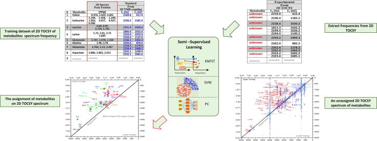
Graphical abstract
Keywords: Machine learning, Semi-supervised learning, Metabolic profiling, 2D TOCSY, NMR spectra, Pattern recognition
Abbreviations: TOCSY, Total Correlation Spectroscopy; KNFST, Kernel Null Foley–Sammon Transform; SVM, Support Vector Machines; PC, Polynomial Classifier; CPMG, Carr-Purcell-Meiboom-Gill; JRES, J-RESolved Spectroscopy; HSQC, Heteronuclear Single Quantum Coherence; SSL, Semi-Supervised Learning; MAS, Magic Angle Spinning
Highlights
-
•
Automatic assignment of metabolites of 2D-TOCSY NMR spectra.
-
•
Semi-supervised learning for metabolic profiling.
-
•
Deconvolution and metabolic profiling of 2D NMR spectra using Machine Learning.
-
•
Accurate Automatic multicomponent assignment of 2D NMR spectrum.
Abstract
Metabolomics is an expanding field of medical diagnostics since many diseases cause metabolic reprogramming alteration. Additionally, the metabolic point of view offers an insight into the molecular mechanisms of diseases. Due to the complexity of metabolic assignment dependent on the 1D NMR spectral analysis, 2D NMR techniques are preferred because of spectral resolution issues. Thus, in this work, we introduce an automated metabolite identification and assignment from 1H-1H TOCSY (total correlation spectroscopy) using real breast cancer tissue. The new approach is based on customized and extended semi-supervised classifiers: KNFST, SVM, third (PC3) and fourth (PC4) degree polynomial. In our approach, metabolic assignment is based only on the vertical and horizontal frequencies of the metabolites in the 1H–1H TOCSY. KNFST and SVM show high performance (high accuracy and low mislabeling rate) in relatively low size of initially labeled training data. PC3 and PC4 classifiers showed lower accuracy and high mislabeling rates, and both classifiers fail to provide an acceptable accuracy at extremely low size (≤9% of the entire dataset) of initial training data. Additionally, semi-supervised classifiers were implemented to obtain a fully automatic procedure for signal assignment and deconvolution of TOCSY, which is a big step forward in NMR metabolic profiling. A set of 27 metabolites were deduced from the TOCSY, and their assignments agreed with the metabolites deduced from a 1D NMR spectrum of the same sample analyzed by conventional human-based methodology.
1. Introduction
The study of metabolism (usually termed “metabolomics”) is an expanding field of medical diagnostics. Many diseases result in an altered metabolism (“metabolic reprogramming”). Metabolic profiling offers insights into the molecular mechanisms of diseases, which provides a sound basis for identifying diagnostic and prognostic biomarkers and rational drug design[1]. Even at early stages, tumors have been found to modify the metabolic profiles of biofluids like e.g., blood and urine, and tissues, resulting in fluctuations of the concentrations of already existing markers or the generation of new ones [1]. On early stages, breast cancer has a curability rate of 70–80%, nevertheless, progressed breast cancer can be mortal [2]. NMR has been used to study metabolic alteration related to breast cancer through detecting the potential and common metabolic signature for early diagnosis and prognosis evaluation, improving the realization of the metabolic pathobiology of breast cancer for supporting the prediction of the cancer development and planning tumor surgical procedures [3], [4], [5], [6], [7].
Nuclear Magnetic Resonance (NMR) spectroscopy has proven to be of high value for identifying the components of complex mixtures of small molecules, like, e.g., metabolites [1]. Therefore, using NMR as an analytical technique has gained increasing interest since it is a non-invasive and highly accurate method that mainly stems from the linear relationship between the area of the peaks in the NMR spectrum and the concentration of the associated species [8].
However, consistent metabolic identification in biological fluids, such as blood and urine or tissue [8], from the 1D NMR spectra is one of the significant challenges since it requires deconvolution of the NMR spectrum to overcome the spectral superposition of several metabolites [9]. Additionally, the signals of each metabolite in a 1H NMR spectrum often overlap, and the peaks shift due to pH and ionic strength variations of the biological matrix [9], [10]. In principle, metabolic identification might be achieved by separating the mixture components by physical means, followed by NMR measurements of each component. In this approach, the overall NMR spectrum is assumed to correspond to a weighted sum of individual metabolite spectra measured individually or taken from an available reference dataset. Accordingly, concurrent metabolic identification by accurately matching the measured metabolites in the sample with the peak positions of the reference spectra can be achieved [10]. This approach is performed manually and involves considerable experience in NMR spectroscopy, metabolic assignment, and the sample type and is prone to operator bias [9], [10]. Moreover, this procedure is not only time-consuming, labor-intensive, and impractical but might also be invasive since some metabolites may lose their activity during separation [11]. Therefore, samples are measured without chemical separation into individual metabolites, and afterward, the deconvolution of the resulting NMR spectrum is performed based on specific approaches such as “targeted metabolite fitting” [10], [12], [13]. Fortunately, in many cases, peaks that overlap in 1D NMR spectra can be resolved in 2D NMR spectra due to their higher spectral dispersion [8], [14]. Therefore, 1H–1H TOCSY (total correlation spectroscopy) is well suited for spectral dispersion. Consequently, the metabolomics assignments can be achieved as the signals of each metabolite occur on a single line (1D cross-sections (row) in the TOCSY spectrum). This approach eases the task of assignment as well as computational analysis. Currently, analyzing the metabolites contained in biological mixtures using TOCSY spectra in an automated or computerized way biological mixtures using TOCSY spectra is limited [8]. Despite that, many existing methods can decompose the mixed-signal spectrum into the individual spectra of the constituent metabolites. However, they cannot cope with the presence of spectral components induced by chemical shifts and overlapping of metabolites because this source of “noise” leads to poor decomposition results. In this article, we introduce the concept of semi-supervised learning (SSL) and the implementation of our own modified classifiers to analyze and identify metabolites of real breast cancer tissue samples based on TOCSY spectra by integrating the concept of confidence bands during the SSL classification process.
2. Analysis concept and related work
Metabolic NMR spectral resonance patterns are available in online databases. By incorporating this information into a Bayesian model, NMR spectral resonance peaks can be deconvolved to identify metabolites and measure their concentrations [9]. The reference NMR spectra are stored in the form of chemical shifts, J-couplings, and multiplet intensity ratios [9]. These properties are used in the sense of a priori probability in a Bayesian framework, allowing for slight deviations of the observed spectral parameters from those of the reference spectra due to pH and ionic strength. The problem of Bayesian analysis of 1D NMR spectra has been solved [9], and the corresponding software is available as the “BATMAN” module in the R environment. 1D NMR spectroscopy is commonly used for molecular assignments of chemical substances in solution [15]. However, in complex mixtures of chemical species such as in metabolomics, strong peak overlaps are encountered, and then 2D NMR is an alternative approach since peak superposition in 1D NMR spectra can often be separated in 2D NMR spectra [8]. Two-dimensional J-resolved (2D JRES) NMR spectroscopy is a favorable technique for analyzing metabolite mixtures as it allows for a record of a second spectral dimension with little overlap between the signals [16]. Moreover, a software tool has been suggested for the combined investigation of 1D and 2D JRES spectra [10]. However, the number of metabolites that can be automatically identified is strongly limited by the spectral resolution of 2D-JRES.
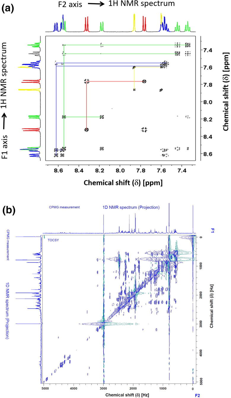
Moreover, strong coupling effects influence this method, especially when the NMR magnetic field is weak. The 2D HSQC [15], [17] technique offers another parameter for the deconvolution of an overlapped signal by incorporating 13C chemical shift information. Therefore, a computational approach for automatic deconvolution employing Fast Maximum Likelihood Reconstruction has been introduced [17]. However, the sensitivity of HSQC is generally inadequate for metabolomics studies [18]. Furthermore, there is the disadvantage of missing spin system information, as all cross-peaks are independent of each other in HSQC and 2D-JRES spectra [19]. On the other hand, in 2D 1H–1H TOCSY spectra, cross-peaks (Fig. 1) of the spin system of one metabolite show up on horizontal and vertical lines in a spectrum, which allows identification of individual 1H spin systems [20]. For this reason, TOCSY is appropriate for computational analysis and spectral assignment [21] of 2D NMR spectra.
Fig. 1.
(a) Simulated 2D Total Coherence Spectroscopy (2D TOCSY) 1H–1H TOCSY spectrum for samples of proton groups (color-coded) in metabolites. Signals belonging to a particular metabolite occur along horizontal (and vertical) lines in the spectrum [21]. (b) The 1H–1H TOCSY spectrum of a real breast cancer tissue sample at 600.13 MHz with τm of 80 ms. and relaxation time of 1 s, 16 K, and 128 data points acquired in the horizontal and the vertical dimension (F2, F1), resp. The NMR projections on F1 and F2 axes are an extra 1D NMR spectrum acquired using the CPMG pulse sequence with excitation sculpting water suppression.
Fig. 1a displays a 2D 1H–1H TOCSY simulated experiment for samples of proton groups (color-coded) in metabolites (according to Simpson [21]). The blue proton group consists of the signals at 8.62, 7.55, 7.59, and 8.56 ppm, whereas the green proton group appeared at 8.54, 7.34, 7.44, and 8.17 ppm. The signals appearing at 7.76 and 8.32 ppm belong to the proton group indicated in red and consist of two protons with a three-bond coupling constant of 8.9 Hz. The signals of the proton group designated in yellow are of two protons and have a small coupling constant of 1.9 Hz, which corresponds to a four-bond correlation [21]. Signals belonging to the particular protons of a metabolite occur along horizontal (and vertical) lines in the spectrum.
Fig. 1b shows the 1H–1H TOCSY spectrum of a real breast cancer tissue sample studied in this work at 600.13 MHz with mixing times (τm) of 80 ms. The 2D TOCSY spectra were recorded using a pulse sequence that suppresses zero-quantum coherences [22] to avoid blurring the multiplet patterns with a relaxation delay of 1 s. In this way, the resulting multiplets exhibit the same structure as in 1D NMR spectra, which facilitates classification. Measurements with a high indirect frequency resolution can only be obtained for a subdivision into many time increments, resulting in long measurement cycles. The spectral range was set to 7 kHz in both dimensions, 16 K and 128 data points acquired in the horizontal and the vertical dimension (F2, F1), respectively. Before 2D Fourier Transform, zero filling were performed to 32 K and 1 K data points in the horizontal and vertical dimensions. The spectral widths in the two dimensions were 12.00 ppm, the spectral width of 8.33 ppm (5000 Hz) is enlarged since TOCSY cross-peaks of the metabolites of the sample appeared in the enlarged spectral width. The NMR experiment has been acquired at temperature of 279 K.
The spectral deconvolution is based on identifying traces overlapping with signals of other spin systems to be directly compared with an NMR database. The 1D NMR spectral projections on the F1 and F2 axes are external projections evoked from extra 1D NMR measurement using the CPMG pulse sequence with embedded water suppression by excitation sculpting. CPMG was used to suppress macromolecules (protein and lipids), and it was recorded employing 400 echoes with 1 ms echo time. The TOCSY chemical shifts of both F2 and F1 were calibrated according to the alanine diagonal peak and set to 1.46 ppm.
The manual spectral deconvolution is dependent on user experience, which is a severe bottleneck in the field [17], [23]. Additionally, it is an impractical and tedious process, especially for high-throughput applications and complex biological mixtures [24], [25]. Semi-automated approaches have been developed to decompose TOCSY spectra into individual mixture components matching in NMR databases for identification [20]. DemixC is a semi-automated technique that deduces 1D cross-sections (row) of a 2D TOCSY spectrum that does not exhibit many peak overlaps [20], and peak fitting is used to extract peak positions from a TOCSY spectrum [20]. Frequently, metabolomics samples are composed of hundreds of individual components, which may result in overlapping peaks and, consequently, problems of the DemixC method [20]. Therefore, the Demixing by Consensus Deconvolution and Clustering (DeCoDeC) is a preferable approach to deal with mixtures of higher complexity[26]. DeCoDeC identifies peaks apparent in specific pairs of TOCSY 1D cross-sections so that overlapping peaks associated with other metabolites are eliminated [20]. Significant limitations of both approaches are the peak shifts due to matrix effects which is the common case in metabolic profiling investigation of real-time evolution measurements [24].
Machine learning is defined as building a classification system that can distinguish between classes and generalize from training models to predict unseen samples [27]. Typically, a machine learning system uses three types of datasets: The first data type is the training dataset which is the labeled training data used to build a generalization model. The second data type is the test dataset which is the unlabeled data to be learned [27]. A third dataset, the validation dataset, is used to tune the parameters of the classifiers. Importantly, all datasets must belong to the same distribution. The trained system uses the generalized model to predict the labels of the unlabeled data. In situations where labeled data is scarce or when the process of labeling large amounts of data is time-consuming and expensive, Semi-Supervised Learning can be used [28].
In Semi-Supervised Learning (SSL), sometimes called self-training, a classifier uses its prediction to update its training model [29]. The system is provided with a limited amount of labeled train data , the associated labels and unlabeled train dataset . In the self-training scenario, the classifiers build a training model based on in the training phase. Later, in the learning phase, a new subset of instances is selected to predict the labels of this subset, where is the number of subsets. Then the subset is removed from and added together with the predicted labels to the training dataset . Finally, the classifier is re-trained using and the labeled subset . This process is repeated until the whole set is exhausted or no confident predictions can be further added to the training dataset [29]. Self-training is used as a wrapper method, so the prediction function is not restricted to specific classifiers, and any classifier can be wrapped in the self-training scenario [29]. On the other hand, self-learning classifiers are sensitive to mislabeling; a wrong prediction can boost itself, affecting the retrained model and the overall performance [29]. A vital element in the self-training method is the confidence measure used to select which is added to the training set. Only the most confident label predictions are added to the training dataset and used to update the training model [28], [29].
Confidence bands are uncertainty measures of an estimate obtained from limited data, and they define the area where the true model lies with probability . Usually, α is set to 0.05, which means we are confident that our model is enclosed by the confidence band [30]. The assured predictions in SSL can be employed by introducing confidence bands, which are used to reject possible outliers, i.e., do not lie in the confidence band threshold [31]. Therefore, samples that lie within the confidence threshold are added to the training set, and then, retraining of the classifier is performed using the added data [31]. Confidence bands can be calculated in several ways, for instance, using Monte Carlo [32] or bootstrapping [33]. Confidence bands were used in the field of SSL to add certainty to the prediction in gesture recognition [34], [35] and image classification [31]. In this work, we use the output of the proposed classifiers to compute the confidence bands following the established procedure presented in the literature [36], [37], [38]. The confidence band of the classifier output for a test sample is measured by
| (1) |
where is the inverse cumulative t-student distribution, is the probability of the chosen confidence band, we use = 0.05 for 95% confidence bands, and is the number of degrees of freedom associated with the t-student distribution. The term represents the covariance matrix computed by finding the weighted Jacobian where and is the associated uncertainty of the sample label that may result from a human or self-training. The residual is the difference between the predicted value and the real value of sample and are the parameters of the classifiers to be optimized [36].
3. Classification methods
In the context of SSL for metabolic profiling of 2D TOCSY NMR spectra, we present the polynomial classifier, support vector machines, and Kernel Null Foley–Sammon Transform classifiers. SSL with confidence bands for images and traffic sign classification using the polynomial classifier and support vector machines has been described in the literature [31], [36]. In this work, we customized these classifiers for metabolic profiling. In addition, we have extended the KNFST classifier to be used in SSL scenarios by employing the concept of confidence bands.
3.1. Polynomial classifier (PC)
Let be the number of training samples X, where of C different classes and class labels . The polynomial classifier takes the following form [39]
| (2) |
where is the polynomial structure representing all the possible multiplicative combinations of the original feature depending on the polynomial degree. The coefficient/weight matrix is obtained during the training phase and is employed during the learning process to obtain the probability that a given feature belongs to class . The polynomial discriminant function creates a mapping from the feature space to a decision space that produces an output of posterior probability estimate to determine the class membership [39]. In this work, we implemented third and fourth-order polynomial classifiers, thus contains linear, quadratic, and cubic multiplicative combinations of the original feature vector. The quadratic multiplicative combination will be employed as well in the case of a fourth-order polynomial function. The model can be solved using least mean squares optimization through minimizing the residual [39].
The Moore-Penrose pseudo-inverse approximation is used to estimate the model parameters during the training phase [27]. In the learning phase, the estimated weight matrix is used to find the label of the new sample [27], [36], [39]. The number of free parameters in the confidence bands calculation is computed according to , where L is the number of classes and M is the number of terms in the polynomial function [36].
3.2. Support vector Machines (SVM)
SVM performs a nonlinear mapping of the original feature vector into a higher-dimensional space and tries to find an optimized hyperplane to separate non-linearly separable data [40]. The support vectors are training samples that act as decision boundaries for the optimal hyperplane [27]. SVM finds this hyperplane by solving
| (3) |
where is high-dimensional non-linear mapping of the features X and is the coefficient matrix, and b is the bias vector. The hyperplane is optimized during the training phase by finding and b, which maximize the distance between the support vectors from each class and the hyperplanes [27]. Only equation (3) has to be computed for every new instance in the learning phase.
The implicit features mapping where is a high dimensional inner-product space, can be used to define a kernel function by [27]. Kernels are widely used in machine learning to implicitly map the original data space into a higher dimension where it is expected to give a better separation for non-linearly separated data [27], as depicted in Fig. 2. Throughout this work, the Gaussian radial basis function (RBF): is used in the classification process, where controls the bandwidth of the kernel function, and it is optimized during the training process [27]. We use the implementation of SVM from the toolbox LIBSVM [42]. Moreover, the confidence bands are calculated using equation (1), the degree of freedom is defined as the difference between the total number of training samples and the number of support vectors [36].
Fig. 2.
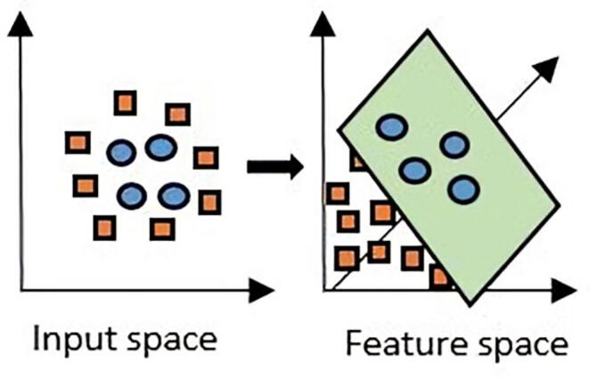
Linear classification cannot separate the blue circles from the orange squares in two dimensions (left). By mapping the original linear feature space to a higher dimension, a plane that separates the data into two classes can be found (right) [41]. (For interpretation of the references to color in this figure legend, the reader is referred to the web version of this article).
3.3. Kernel null Foley–Sammon Transform (KNFST)
KNFST finds the projection direction that achieves the best separately between classes by minimizing the within-class scatter and maximizing the between-class scatter . Consequently, a sample is projected as close as possible to samples that belong to the same class and as far as possible to samples that belong to a different class [43], [44]. KNFST is defined as
| (4) |
By enforcing the conditions and in equation (4), we get a projection direction that guarantees the best separability between classes in a higher-dimensional space [43], [44] as shown in Fig. 3.
Fig. 3.
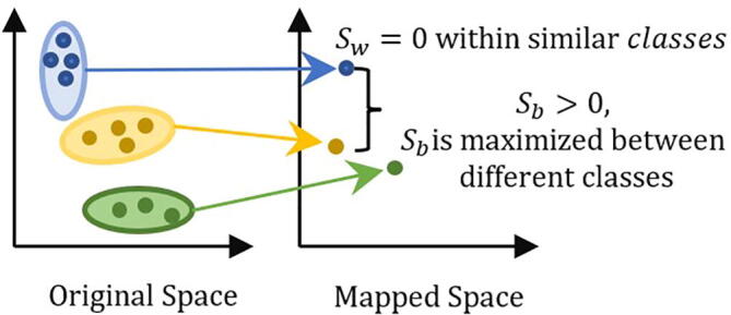
Geometrical visualization of KNFST, where every class is mapped into a single point. Test samples are mapped nearer to the class representation they belong to and far away from different classes.
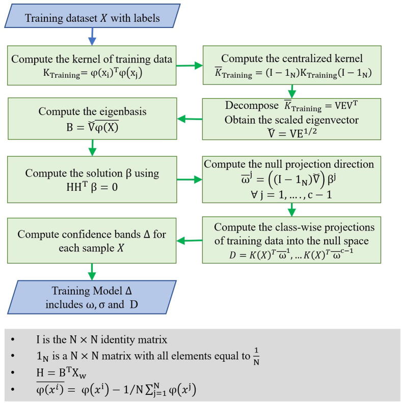
KNFST has used an outlier detection in previous work [43], [45], [46]. Nevertheless, in this work, we have extended the functionality of KNFST to be employed in the SSL scenario as follows: During the training phase, the projection direction , the class-wise projections of training data into the null space [43], in addition to the confidence band for each sample are computed using the training data. During the learning process, for each sample , the projection using is computed. The class membership is computed according to
| (5) |
In equation (5), the class membership is computed by calculating the Euclidean distance between the projected sample and the projection of all classes in the mapped null space. The instance is assigned to the nearest class, as depicted in Fig. 4. Next, the confidence band for is computed according to equation (1). The degree of freedom for the t-student distribution is the difference between the size of the feature space and the size of the projected dimension [47].
Fig. 4.
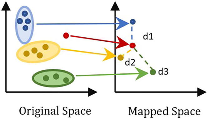
Class membership is determined according to the distance between the projected class and the new red sample. The blue, yellow, and green classes are mapped into one point for each class in the mapped class. The assignment of the new red sample is determined according to the distance between its projection and the projection of the other classes (d1, d2, d3). The distance d2 is the shortest distance to the red class. Therefore, it is more probable that the red sample belongs to the yellow class. (For interpretation of the references to color in this figure legend, the reader is referred to the web version of this article).
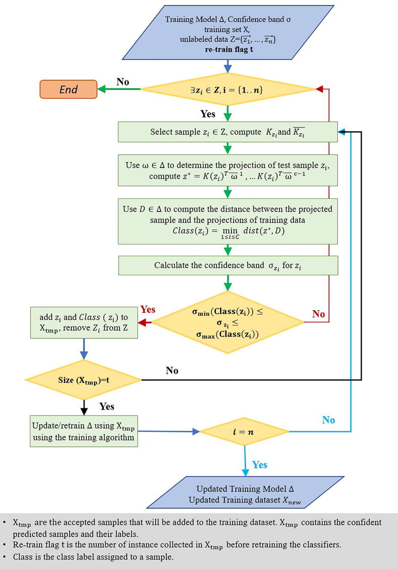
Initially, confidence bands are computed from the training data, and their values are the main criterion to decide whether a sample is used to update the training set. A relative deviation of the confidence value of training data is allowed, i.e., an unlabeled sample can be added to the training set once its corresponding confidence value falls within this deviation. Once the sample is accepted, it is added to the training set together with its label and confidence value. At last, the classifier is retrained after a maximum of t samples has been added. For the sample , we construct a two-sided normalized confidence band using a bootstrap method such that probability, where is the computed confidence band for sample . The values of and are calculated as , and , where and are experiment-dependent and is the confidence band vector of the training data. Generally, all possible combinations values could be examined [48]. In our settings, if multiple combinations of and achieve a similar accuracy and misclassification rate, then we choose the configuration with the narrowest confidence band. Fig. 5 and Fig. 6 summarize and demonstrate the steps in training and the learning phases of KNFST, respectively.
Fig. 5.
The training phase in semi-supervised KNFST algorithm. The training phase aims to generate a training model based on the training dataset. The training models consist of the optimized projection matrix, confidence bands values, and the class-wise projections of training data into the null space.
Fig. 6.
Learning phase in semi-supervised KNFST algorithm. The learning process starts by using the pre-generated training model. SSL iteratively selects a sample from the unlabeled data. The classifier predicts a label for the sample where new labels are accepted if the confidence band value is within a range . Those accepted samples are added to the initial training set and their predicted labels after accepted samples, where is a re-train flag used to check the number of accepted samples before retraining the classifier. The classifier is retrained on those samples, creating a new training model that will be used to predict the labels for the rest of the unlabeled data. This procedure is repeated until no more unlabeled data matches the confidence band conditions. If there is no qualified example left, the algorithm terminates.
4. Dataset
4.1. Acquisition and preprocessing
1D and 2D TOCSY NMR spectra were acquired experimentally on a real breast cancer tumor tissue sample [49] by employing a broadband high resolution 600.13 MHz (B0 = 14.1 T) NMR Bruker spectrometer (AVANCE III 600 with the Bruker magnet ASCEND 600) supported with the room temperature probe (BBO model-Bruker) and Magic Angle Spinning (MAS) probehead. 1D and 2D NMR spectra acquisition and processing were achieved by using the TopSpin software package 3.6.
1D NMR spectrum of the sample was measured, analyzed, and assigned based on expert knowledge with the help of the Chenomx NMR Analysis Software from (Chenomx Inc.). A number of 27 metabolites were assigned in the measured real breast cancer tissue sample as following, namely: ’Valine’, ’Isoleucine’, ’Leucine’, ’Lysine’, ’Glutamate’, ’Alanine’, ’Glutamine’, ’Aspartate’, Sn-Glycero-3-phosphocholine (GPC), ’Serine’, ’O-Phosphoethanolamine’, ’Ascorbate’, ’Myo-Inositole’, ’Lactate’, ’Proline’, ’3-Hydroxybutyrate’, ’O-Phosphocholine’, ’Threonine’, ’Glutathione’, ’Inosine’, ’Beta-Glucose’, ’Alfa-Glucose’, ’Tyrosine’, ’Phenylalanine’, ’Uracil’, ‘Taurine’ and ’Methionine’.
The 2D TOCSY spectra were recorded, as mention earlier.
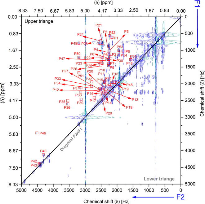
The peak (F2, F1 in Hz) entries are deduced from the experimental 2D TOCSY NMR spectrum (shown in Fig. 1b and explained earlier) of the real breast cancer tissue from the 2D contour lines using the automatic peak picking function (pp2d) in Bruker TopSpin 3.6. The peaks picking level was adjusted based on the contour projection magnitude threshold to avoid picking artifacts and noise peaks. Peaks are annotated on the TOCSY spectrum using the red square symbol associated with peak number, as illustrated in Fig. 7. The peaks are listed and transferred as a text file to the semi-supervised classifiers programmed in Matlab for the successive analysis.
Fig. 7.
The peaks deduced from the experimental 2D TOCSY NMR spectrum (shown in Fig. 1b) from the 2D contour lines using the automatic peak picking function (pp2d) in Bruker TopSpin 3.6. The peak picking level was adjusted according to the contour projection magnitude threshold to avoid picking artifacts and noise peaks. Peaks are annotated in the TOCSY spectrum using the red square symbol associated with the peak number. (For interpretation of the references to color in this figure legend, the reader is referred to the web version of this article).
4.2. Data representation
In our datasets, each metabolite is represented by two main characteristic features of the 2D TOCSY spectra: the chemical shift frequencies on the horizontal and vertical axes, respectively. Since sufficient data samples is a vital element for classification, data augmentation is implemented in this work to overcome the small datasets due to limited NMR data [50], [51]. Data augmentation is implemented to extend the number of data samples by simulating anticipated deviation on the original samples [52]. Thus, data augmentation results in duplicates of the samples, and the classifiers will deal with the same sample in different versions [53]. Data augmentation has been applied in spectrum classification in NMR [54], Raman spectra [52], and infrared spectra [55]. Before starting the classification process, the data augmentation is used to create four disjoint datasets, training and validation, learning and testing sets. Each dataset will have 1200 data instances. In the training dataset, white Gaussian noise is added to the original frequencies with a different random signal-to-noise ratio. In the learning set, random noise is added to each instance of the original dataset. The validation and testing datasets are created by shifting the horizontal and the vertical frequency by a random value under a predetermined chemical shift constraint, within 30 Hz, 0.049 ppm, which is sufficiently more than the limit chemical shift fluctuation due to the NMR environmental matrix change [56]. An example of the data augmentation procedure for proline is shown in Table 1.
Table 1.
A subset of the training dataset showing the output of the data augmentation procedure for proline. From one standard chemical shift for a metabolite, multiple versions of the same metabolite can be created.
| Chemical shift | ||||
|---|---|---|---|---|
| Experimental | Augmented | |||
| Metabolite | Horizontal freq. | Vertical freq. | Horizontal freq. | Vertical freq. |
| proline | 2471.9 | 1402.2 | 2476.29 | 1399.85 |
| 2474.27 | 1398.34 | |||
| 2468.91 | 1400.06 | |||
| 2472.68 | 1403.74 | |||
| 2469.03 | 1398.45 | |||
| 2470.36 | 1404.45 | |||
| …… | …… | |||
| …... | …… | |||
5. Experiments
In the scenario of semi-supervised learning, a third (PC3) and fourth-order (PC4) polynomial classifier, KNFST, and SVM classifiers are tested. The performance of the classifiers for increasing the size of the initial training set was investigated and plotted in Fig. 8, Fig. 9, Fig. 10, Fig. 11. The learning procedure is repeated for different initial amounts of training data to examine the role of the size of the initial dataset on the learning process and to observe the minimum ratio of the initial training set, which is sufficient to produce an acceptable performance. The labeled dataset is partitioned into ten portions of training data. The system uses random initial training samples, starting from 10%, 20%, 30%, until reaching 100% of the training data.
Fig. 8.
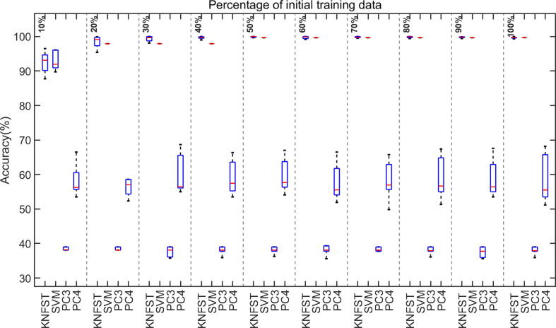
The accuracy of classification versus different sizes of initial training data.
Fig. 9.
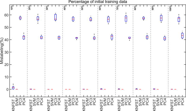
Mislabeling rates versus different sizes of initial training data.
Fig. 10.
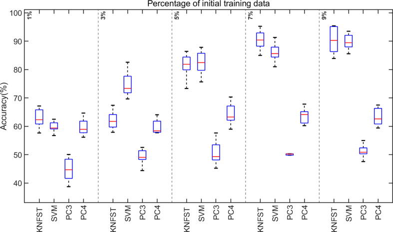
The accuracies of classification versus the size of the initial training data set for small initial amounts of labeled training data (≤9% of the entire dataset).
Fig. 11.
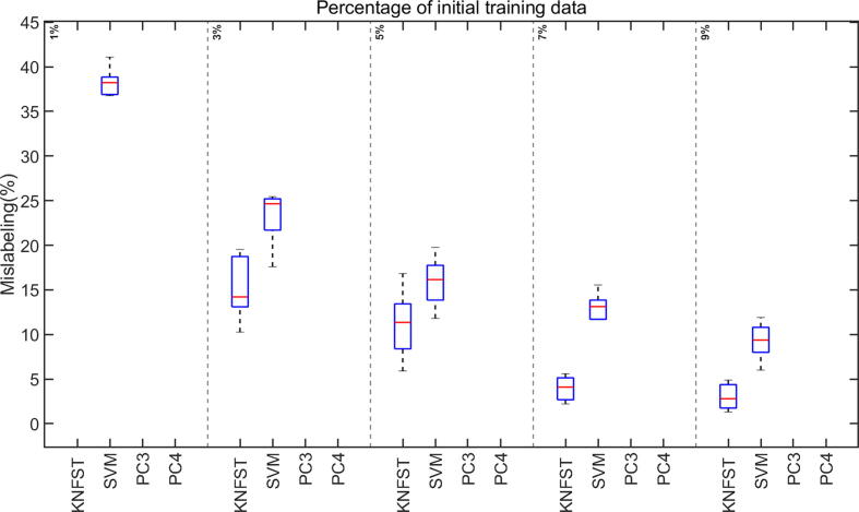
Comparison between the mislabeling rates of class cation using small sizes of the initial labeled training data set.
This random division and permutation of the training dataset will lead to a different number of samples per metabolite; this is important to monitor how classifiers will handle unbalanced datasets in diverse experimental situations. Therefore, it is essential to repeat the experiment multiple times and enforce the classifiers to deal with random permutation and partition to obtain accuracy expectations independent of the partition of the training dataset. The labeled dataset is partitioned into ten portions of training data. The system starts by using random initial training samples, starting from 10%, 20%, 30%, until reaching 100% of the training data size. For each portion of the initial training dataset, ten runs are performed. Thus, the classifiers will perform the experiments ten times for each of the ten partitions of the training dataset.
The assessment of the results is based on the accuracy of the classification: Accuracy = Number of correctly classified samples / Total number of samples and the rate of mislabeled samples added to the training set: Mislabeling rate = Number of wrongly classified samples added to the training set / Total number of learned examples added to the training set.
6. Results and discussion
The accuracy and the mislabeling of the classifiers versus the size of initial training data are displayed as boxplots of median and standard deviation for ten different processing runs. Fig. 8 shows the classification accuracy of KNFST, SVM, PC3, and PC4 classifiers. From the plot, the accuracy of KNFST and SVM increases with an increasing initial amount of labeled data until reaching around 100% at the size of 20% of the initial training dataset, where it is corresponding at this point to only eight samples per metabolite. Conversely, in comparison to KNFST and SVM, PC3 and PC4 showed a lower accuracy and no improvement in the performance with the increasing size of the training dataset. The most probable explanation is the high mislabeling rate, shown in Fig. 9, where PC3 and PC4 have mislabeling rates of around 60% and 45%, respectively, regardless of the sizes of the training dataset. Noticeably, both PC3 and PC4 were unable to learn any samples until using 30% and 40% initial labeled training data. Remarkably, the mislabeling (misclassification) of KNFST and SVM start with a rate of less than 5% (considered significantly low), and it was decreasing with increasing training set size reaching nearly 0%.
Analyzing the performance of the classifiers in the presence of an extremely small amount of initial training data, as low as one or two labeled samples per metabolite, is also noteworthy for this work since an NMR dataset is always kept as small as possible to save measuring time and to avoid sample alteration with time, leading to data scarcity. Fig. 10 shows the accuracy of the classifiers in these cases with only 1% of the training dataset, ensuring one sample per metabolite per multiplet. Interestingly, the accuracy of SVM and KNFST kept increasing steadily despite the extremely small size of the initial training dataset. Additionally, the accuracies of both KNFST and SVM reached 90% at an initial training dataset of size 9%.
The mislabeling rate of the SVM is around 40% at 1% of the initial training dataset, as shown in Fig. 11. No mislabeling rates appear for KNFST because it was not able to learn any sample. Later on, the values of mislabeling of KNFST and SVM were around 15% and 25%, respectively. These values of mislabeling were decreasing with increasing initial training data set size. Within the low training data set size settings, KNFST showed a higher performance than SVM, while both showed better accuracy than PC3 and PC4 at extremely low size settings. The mislabeling rates of PC3 and PC4 for extremely low sizes of the initial training data could not be defined (see Fig. 11). This is typical for polynomial classifiers since they commonly require a relatively large amount of training data in order to be able to generalize [36]. It is essential that when a classifier is unable to learn any data samples and hence does not appear on the figures, the whole classification process turns into a supervised learning procedure rather than semi-supervised learning. This happens because no new data samples will be added to the initial training data set when the classifier does not learn any sample. Therefore, the test dataset will be tested against the un-updated original training data set. This explains the accuracies that appear in Fig. 10 despite the absence of mislabeling in Fig. 11.
7. Validation
The metabolite assignments of the breast cancer sample were validated based on the matching between the metabolites standard chemical shift from 1D NMR and 2D TOCSY with the experimental 2D TOCSY on the same sample (breast cancer tissue). Every metabolite 2D TOCSY standard chemical shift was deduced from the standard chemical shift 1D NMR from the BATMAN [9], BMRB [57], and HMDB [58] databases as well as relevant literature [59], [60].
Standard (F2, F1) cross-peak entries of 1H–1H TOCSY of the metabolites that appeared in the studied breast cancer tissue are listed in Table 2. Standard entries (indicated in the table) were deduced from the coupled peaks that appeared in standard 1D NMR spectra from affirmed databases as well as standard 2D TOCSY [1], [9], [57], [58], [59], [60]. Experimental cross-peaks are deduced from the measured TOCSY of the sample. Characteristic (F2, F1) cross-peak entries of every metabolite that has been used for the assignment are listed. These peaks are labeled with P1 until P48, and they are annotated in Fig. 7.
Table 2.
Standard and experimental (F2, F1) Hz cross-peak entries of 1H–1H TOCSY of the metabolites appeared in the studied real breast cancer tissue. Standard entries (indicated in the table) were deduced from the coupled peaks that appeared in standard 1D NMR spectra from affirmed databases [9], [57], [58], [59], [60]. Experimental (F2, F1) Hz cross-peaks are deduced from the experimental TOCSY measurement of the sample. Only characteristic (F2, F1) Hz cross-peak entries of every metabolite are listed, and they are labeled with P1 to P48 and annotated in Fig. 7.
| 1D SpectraPeak Position | Peak | Standard | Experimental | ||||
|---|---|---|---|---|---|---|---|
| From1D NMR coupling | From2D TOCSY | ||||||
| # | Metabolite | [PPM] | position | F1 [Hz] | F2 [HZ] | F2 [Hz] | F1 [HZ] |
| 1 | Valine | 0.976, 1.029, 3.601 | P1 | 2160.6 | 617.4 | 2159.4 | 615.4 |
| 2 | Isoleucine | 1.249, 1.458, 1.249, 1.969, 3.657, 0.927, 0.998 | P2 | 2194.2 | 1181.4 | 2190.4 | 1182.2 |
| 3 | Leucine | 0.94, 0.953.719, 1.701 | P3 | 2231.4 | 1020.6 | 2238.4 | 1020.2 |
| 4 | Lysine | 1.72, 3.01, 3.751.895 | P4, P5 | 1806.0 | 1032.0 | 1812.3 | 1026.2 |
| 2250.0 | 1032.0 | 2244.4 | 1026.2 | ||||
| 2250.0 | 1137.0 | 2244.4 | 1140.2 | ||||
| 5 | Glutamate | 3.747, 2.078, 2.339 | P6 | 2248.2 | 1403.4 | 2259.2 | 1404.3 |
| 6 | Alanine | 1.46, 3.76 | P7 | 2256.0 | 876.0 | 2262.4 | 882.2 |
| 7 | Glutamine | 3.764, 2.13, 2.447 | P8, P9 | 2258.4 | 1278.0 | 2262.4 | 1278.2 |
| 2258.4 | 1468.2 | 2262.4 | 1464.3 | ||||
| 8 | Aspartate | 3.886, 2.802, 2.651 | P10, P11 | 2332.1 | 1590.9 | 2323.2 | 1602.2 |
| 2332.1 | 1681.6 | 2323.4 | 1685.1 | ||||
| 9 | sn‐glycero‐3-phosphocholine (GPC) | 3.605, 3.672,3.903, 3.871.3.946, 4.312,3.659, 3.212 | P12, P13 | 2587.8 | 2195.8 | 2587.9 | 2210.5 |
| 2342.3 | 2163.5 | 2367.8 | 2117.7 | ||||
| 10 | Serine | 3.833, 3.958 | P14 | 2375.3 | 2300.0 | 2390.2 | 2294.6 |
| 11 | O-phosphoethanolamine | 3.240, 4.014 | P15 | 2408.9 | 1944.4 | 2390.4 | 1941.1 |
| 12 | Ascorbate | 4.857, 4.771, 3.734, 3.440 | P16, P17 | 2240.9 | 2064.4 | 2217.1 | 2090.0 |
| 2405.3 | 2241.5 | 2435.0 | 2204.1 | ||||
| 13 | Myo-Inositole | 3.518, 4.049, 3.611, 3.265 | P18, P19, P20 | 2112.5 | 1959.4 | 2076.8 | 1958.9 |
| 2167.1 | 1959.4 | 2170.2 | 1958.9 | ||||
| 2429.9 | 2112.5 | 2432.1 | 2109.0 | ||||
| 14 | Lactate | 4.104, 1.317 | P21 | 2462.9 | 790.4 | 2468.2 | 787.5 |
| 15 | Proline | 4.119, 3.407, 3.323, 2.002, 2.080, 2.336, 2.022 | P22, P23 | 2471.9 | 1213.2 | 2468.2 | 1217.7 |
| 2471.9 | 1402.2 | 2468.2 | 1389.7 | ||||
| 16 | 3-Hydroxybutyrate | 4.160, 2.414, 2.314, 1.204 | P24, P25, P26 | 2496.0 | 722.4 | 2506.6 | 718.4 |
| 2496.0 | 1388.4 | 2506.6 | 1376.6 | ||||
| 2496.0 | 1448.4 | 2506.6 | 1438.7 | ||||
| 17 | O-Phosphocholine | 4.285, 3.644 | P27 | 2571.6 | 2186.9 | 2550.5 | 2161.1 |
| 18 | Threonine | 4.241, 1.318, 3.573 | P28, P29 | 2545.2 | 791.0 | 2543.6 | 787.7 |
| 2545.2 | 2144.3 | 2543.6 | 2143.4 | ||||
| 19 | Glutathione | 4.557, 2.97, 2.9433.766, 2.548, 2.158 | P30, P31 | 1529.0 | 1295.0 | 1572.0 | 1277.7 |
| 2262.5 | 1295.0 | 2260.7 | 1277.7 | ||||
| 20 | Beta-Glucose | 4.630, 3.230, 3.473, 3.387, 3.450, 3.882, 3.707 | P32, P33, P34 | 2778.6 | 1938.4 | 2788.3 | 1944.4 |
| 2778.6 | 2084.3 | 2788.3 | 2083.8 | ||||
| 2778.6 | 2081.9 | 2788.3 | 2080.3 | ||||
| 21 | Inosine | 8.189, 8.310, 6.066, 4.752, 4.439, 4.278, 3.882 | P35, P36 | 3640.4 | 2567.4 | 3543.4 | 2501.8 |
| 3640.4 | 2664.0 | 2868.5 | 2603.0 | ||||
| 22 | Alfa-Glucose | 5.216, 4.630, 3.519, 3.698, 3.822, 3.826, 3.749 | P37, P38, P39 | 3130.3 | 2112.0 | 3131.9 | 2115.7 |
| 3130.3 | 2224.7 | 3140.2 | 2248.9 | ||||
| 3132.0 | 2568.5 | 3127.7 | 2464.9 | ||||
| 23 | Tyrosine | 7.192, 6.898, 3.200, 3.055, 3.936 | P40, P41 | 23,621 | 1920.4 | 2374.5 | 1920.4 |
| 4316.1 | 4139.7 | 4307.3 | 4124.8 | ||||
| 24 | Phenylalanine | 3.283, 3.113, 3.983, 7.322, 7.420, 7.369 | P42, P43P44 | 4453.0 | 4394.3 | 4443.9 | 4387.0 |
| 4453.0 | 4422.5 | 4443.9 | 4425.9 | ||||
| 2390.3 | 1970.1 | 2384.4 | 1954.8 | ||||
| 25 | Taurine | 3.246, 3.410 | P45 | 2049.9 | 1949.7 | 2078.7 | 1951.2 |
| 26 | Uracil | 5.79, 7.52 | P46 | 4513.0 | 3474.8 | 4513.3 | 3471.7 |
| 27 | Methionine | 3.850, 2.183, 2.122, 2.629 | P47, P48 | 2310.5 | 1308.3 | 2316.6 | 1285.1 |
| 1578.3 | 1308.3 | 1571.4 | 1286.3 | ||||
After the chemical shift verification of the cross-peak entries, the chemical shifts had been assigned to metabolites. The results were verified and confirmed according to the published work on the same sample of the same scientific group [49], [61].
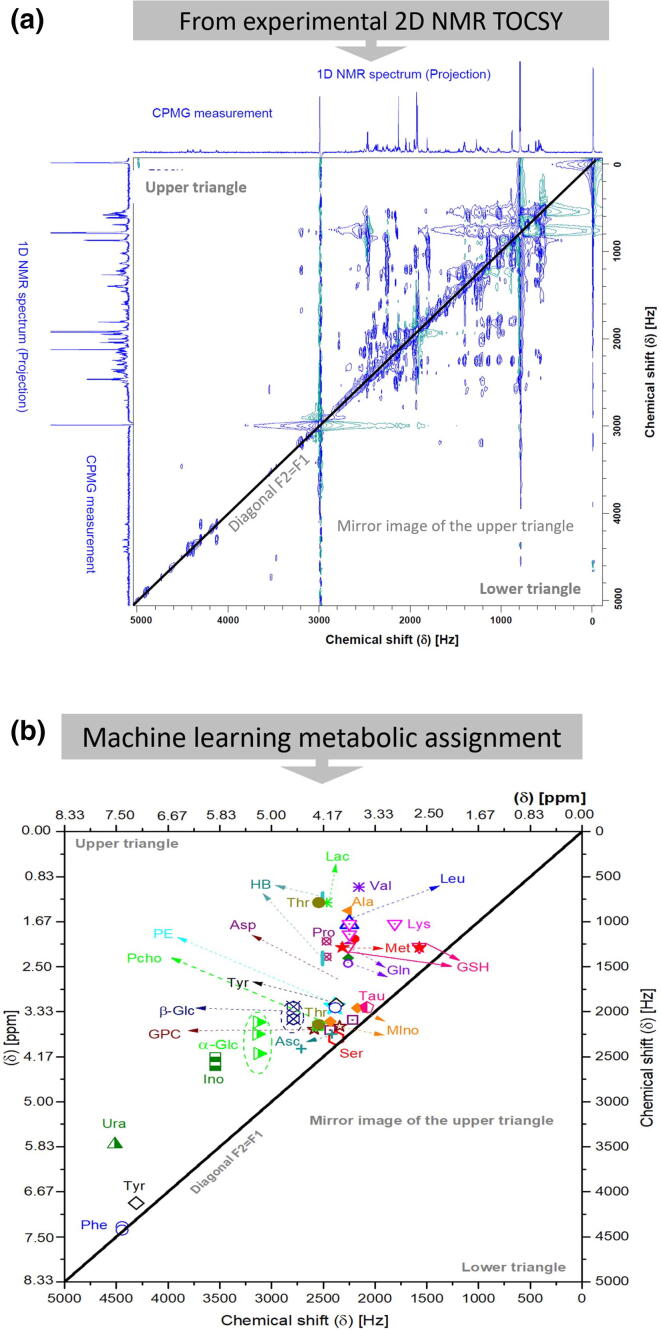
The demonstrated assignment in Fig. 12 was done considering the results of the KNFST classifier only because it has shown the highest accuracy. The metabolite assignment was perfect (100%) without an occurrence of mismatching of the entries. Interestingly, the KNFST classifier matched all metabolites, although, for some metabolites, the chemical shift deviation was around 30 Hz (0.049 ppm), corresponding to a severe deviation that may cause substantial uncertainty in the metabolic assignment.
Fig. 12.
The metabolite assignment based on (a) the experimental 2D TOCSY NMR spectrum of the breast cancer tissue after considering (b) the results of the KNFST classifier, which provides the highest accuracy. Acronyms of the metabolites are Val: Valine; Ile: Isoleucine; Leu: Leucine; Lys: Lysine; Glu: Glutamate; Ala: Alanine; Gln: Glutamine; Asp: Aspartate; GPC: sn‐glycero‐3-phosphocholine; Ser: serine; PE: O-phosphoethanolamine; Asc: ascorbate; mIno: myo-Inositole; Lac: Lactate; Pro: Proline; HB: 3-Hydroxybutyrate; PCho: O-Phosphocholine; Thr: Threonine; GSH: Glutathione; β-Glucose; α-Glucose; Ino: Inosine; Tyr: Tyrosine; Phe, phenylalanine; Tau: Taurine; Ura: Uracil; Met: methionine.
8. Conclusions
This work enabled the automatic and accurate spectral assignment of metabolites based on deconvolution of 2D-TOCSY NMR spectra by employing a semi-supervised machine learning approach. We have customized and extended four semi-supervised learning classifiers to test the automatic assignment under different initial training set sizes. The correctness of the metabolic assignments by our approach in applying 2D TOCSY spectra was based on comparing the results deduced from 1D-NMR spectra by human specialists on the same samples (real breast cancer tissue sample). The KNFST and SVM classifiers show high performance and low mislabeling rates for small and large sizes of the initially labeled training data set. To accept or reject the classification results of the classifiers, the concept of confidence bands was implemented. Under the same settings, both polynomial classifiers show a much weaker performance. For an extremely small size (≤9% of the entire dataset) of the initial training data set, PC3 and PC4 polynomial fail to provide good performance compared to KNFST and SVM classifiers, while the latter provided satisfactory performance as well as a low mislabeling rate. Hence, KNFST and SVM show superior performance over the other tested classifiers at every size of the initial training dataset. Our study demonstrates that machine learning in metabolite assignments based on the 2D TOCSY NMR spectra approach can be considered accurate and robust.
CRediT authorship contribution statement
Lubaba Migdadi: Conceptualization, Methodology, Software, Data curation, Writing - original draft, Visualization, Validation, Formal analysis, Writing - review & editing. Jörg Lambert: Conceptualization, Data curation, Writing - review & editing. Ahmad Telfah: Conceptualization, Visualization, Investigation, Data curation, Writing - original draft. Roland Hergenröder: Conceptualization, Supervision, Writing - review & editing. Christian Wöhler: Conceptualization, Supervision, Writing - review & editing.
Declaration of Competing Interest
The authors declare that they have no known competing financial interests or personal relationships that could have appeared to influence the work reported in this paper.
Acknowledgment
Financial support by the Ministerium für Innovation, Wissenschaft und Forschung des Landes Nordrhein-Westfalen, the Senatsverwaltung für Wirtschaft, Technologie und Forschung des Landes Berlin, and the Bundesministerium für Bildung und Forschung is gratefully acknowledged.
Contributor Information
Lubaba Migdadi, Email: lubaba.migdadi@isas.de.
Roland Hergenröder, Email: roland.hergenroeder@isas.de.
References
- 1.Gowda G.N. Metabolomics-based methods for early disease diagnostics. Exp Rev Mol Diagnost. 2008;8(5):617–633. doi: 10.1586/14737159.8.5.617. [DOI] [PMC free article] [PubMed] [Google Scholar]
- 2.Harbeck N. Breast cancer. Nat Rev Dis Primers. 2019;5(1):66. doi: 10.1038/s41572-019-0111-2. [DOI] [PubMed] [Google Scholar]
- 3.Suman S. Metabolic fingerprinting in breast cancer stages through (1)H NMR spectroscopy-based metabolomic analysis of plasma. J Pharm Biomed Anal. 2018;160:38–45. doi: 10.1016/j.jpba.2018.07.024. [DOI] [PubMed] [Google Scholar]
- 4.Günther U.L. Metabolomics Biomarkers for Breast Cancer. Pathobiology. 2015;82(3–4):153–165. doi: 10.1159/000430844. [DOI] [PubMed] [Google Scholar]
- 5.Cao M.D. Glycerophosphodiester phosphodiesterase domain containing 5 (GDPD5) expression correlates with malignant choline phospholipid metabolite profiles in human breast cancer. NMR Biomed. 2012;25(9):1033–1042. doi: 10.1002/nbm.2766. [DOI] [PMC free article] [PubMed] [Google Scholar]
- 6.Yang L. Application of metabolomics in the diagnosis of breast cancer: a systematic review. J Cancer. 2020;11(9):2540–2551. doi: 10.7150/jca.37604. [DOI] [PMC free article] [PubMed] [Google Scholar]
- 7.Giskeødegård G.F. Lactate and glycine-potential MR biomarkers of prognosis in estrogen receptor-positive breast cancers. NMR Biomed. 2012;25(11):1271–1279. doi: 10.1002/nbm.2798. [DOI] [PubMed] [Google Scholar]
- 8.Emwas A.H. NMR Spectroscopy for Metabolomics Research. Metabolites. 2019;9:7. doi: 10.3390/metabo9070123. [DOI] [PMC free article] [PubMed] [Google Scholar]
- 9.Hao J. Bayesian deconvolution and quantification of metabolites in complex 1D NMR spectra using BATMAN. Nat Protoc. 2014;9(6):1416. doi: 10.1038/nprot.2014.090. [DOI] [PubMed] [Google Scholar]
- 10.Gómez J. Dolphin: a tool for automatic targeted metabolite profiling using 1D and 2D 1H-NMR data. Anal Bioanal Chem. 2014;406(30):7967–7976. doi: 10.1007/s00216-014-8225-6. [DOI] [PubMed] [Google Scholar]
- 11.Davis V.W. Metabolomics and surgical oncology: Potential role for small molecule biomarkers. J Surg Oncol. 2011;103(5):451–459. doi: 10.1002/jso.21831. [DOI] [PubMed] [Google Scholar]
- 12.Zheng C. Identification and quantification of metabolites in 1H NMR spectra by Bayesian model selection. Bioinformatics. 2011;27(12):1637–1644. doi: 10.1093/bioinformatics/btr118. [DOI] [PMC free article] [PubMed] [Google Scholar]
- 13.Peng W.K., Ng T.-T., Loh T.P. Machine learning assistive rapid, label-free molecular phenotyping of blood with two-dimensional NMR correlational spectroscopy. Communications Biology. 2020;3(1):535. doi: 10.1038/s42003-020-01262-z. [DOI] [PMC free article] [PubMed] [Google Scholar]
- 14.Peng, W.K., Clustering Nuclear Magnetic Resonance: Machine learning assistive rapid two-dimensional relaxometry mapping. Eng Rep n/a(n/a): p. e12383.
- 15.Bingol K. Unified and isomer-specific NMR metabolomics database for the accurate analysis of (13)C-(1)H HSQC spectra. ACS Chem Biol. 2015;10(2):452–459. doi: 10.1021/cb5006382. [DOI] [PMC free article] [PubMed] [Google Scholar]
- 16.Aue W.P., Karhan J., Ernst R.R. Homonuclear broad band decoupling and two-dimensional J-resolved NMR spectroscopy. J Chem Phys. 1976;64(10):4226–4227. [Google Scholar]
- 17.Chylla R.A. Deconvolution of two-dimensional NMR spectra by fast maximum likelihood reconstruction: application to quantitative metabolomics. Anal Chem. 2011;83(12):4871–4880. doi: 10.1021/ac200536b. [DOI] [PMC free article] [PubMed] [Google Scholar]
- 18.Fardus-Reid F., Warren J., Le Gresley A. Validating heteronuclear 2D quantitative NMR. Anal Methods. 2016;8(9):2013–2019. [Google Scholar]
- 19.Mauve C. Sensitive, highly resolved, and quantitative 1H–13C NMR data in one go for tracking metabolites in vegetal extracts. Chem Commun. 2016;52(36):6142–6145. doi: 10.1039/c6cc01783e. [DOI] [PubMed] [Google Scholar]
- 20.Bingol K., Brüschweiler R. Multidimensional approaches to NMR-based metabolomics. Anal Chem. 2014;86(1):47–57. doi: 10.1021/ac403520j. [DOI] [PMC free article] [PubMed] [Google Scholar]
- 21.Simpson, J.H., Organic structure determination using 2-D NMR spectroscopy: a problem-based approach. 2011: Academic Press.
- 22.Thrippleton M.J., Keeler J. Elimination of zero-quantum interference in two-dimensional NMR spectra. Angew Chem Int Ed. 2003;42(33):3938–3941. doi: 10.1002/anie.200351947. [DOI] [PubMed] [Google Scholar]
- 23.Qu X. Accelerated Nuclear Magnetic Resonance Spectroscopy with Deep Learning. Angew Chem Int Ed. 2020;59(26):10297–10300. doi: 10.1002/anie.201908162. [DOI] [PubMed] [Google Scholar]
- 24.Cherni A. Challenges in the decomposition of 2D NMR spectra of mixtures of small molecules. Faraday Discuss. 2019;218:459–480. doi: 10.1039/c9fd00014c. [DOI] [PubMed] [Google Scholar]
- 25.Snyder D.A., Zhang F., Brüschweiler R. Covariance NMR in higher dimensions: application to 4D NOESY spectroscopy of proteins. J Biomol NMR. 2007;39(3):165–175. doi: 10.1007/s10858-007-9187-1. [DOI] [PubMed] [Google Scholar]
- 26.Bingol K., Brüschweiler R. Deconvolution of Chemical Mixtures with High Complexity by NMR Consensus Trace Clustering. Anal Chem. 2011;83(19):7412–7417. doi: 10.1021/ac201464y. [DOI] [PMC free article] [PubMed] [Google Scholar]
- 27.Bishop C.M., Recognition P., Learning M. Springer-Verlag; Heidelberg: 2006. Berlin. [Google Scholar]
- 28.Chapelle, O., Schlkopf, B. Zien, A. Semi-Supervised Learning; 2010: The MIT Press.
- 29.Zhu X., Goldberg A.B. Introduction to Semi-Supervised Learning. Synth Lect Artif Intellig Mach Learn. 2009;3(1):1–130. [Google Scholar]
- 30.Foster C. Confidence trick: the interpretation of confidence intervals. Canad J Sci, Mathemat Technol Educat. 2014;14(1):23–34. [Google Scholar]
- 31.Hillebrand, M., et al. Self-learning with confidence bands. in Proc. 20th Workshop Computational Intelligence. 2010. Citeseer.
- 32.Kendall W.S., Marin J.-M., Robert C.P. Confidence bands for Brownian motion and applications to Monte Carlo simulation. Statist Comput. 2007;17(1):1–10. [Google Scholar]
- 33.Bluhmki T. A wild bootstrap approach for the Aalen-Johansen estimator. Biometrics. 2018;74(3):977–985. doi: 10.1111/biom.12861. [DOI] [PubMed] [Google Scholar]
- 34.Al-Behadili, H., et al. Semi-supervised learning using incremental support vector machine and extreme value theory in gesture data. in 2016 UKSim-AMSS 18th International Conference on Computer Modelling and Simulation (UKSim); 2016. IEEE.
- 35.Al-Behadili, H., A. Grumpe, and C. Wöhler. Non-linear Distance-based Semi-supervised Multi-class Gesture Recognition. in VISIGRAPP (3: VISAPP); 2016.
- 36.Cui, T., et al. Analytically tractable sample-specific confidence measures for semi-supervised learning. in Proc. Workshop Computational Intelligence; 2011.
- 37.Martos A., Krüger L., Wöhler C. in Proc. of the 4th Int. Symp. on 3D Data Processing, Visualization and Transmission (3DPVT) 2010. Towards Real Time Camera Self Calibration: Significance and Active Selection. [Google Scholar]
- 38.Kardaun, O.J., Classical methods of statistics: with applications in fusion-oriented plasma physics. 2005: Springer Science & Business Media.
- 39.Schürmann, J., Pattern classification: a unified view of statistical and neural approaches. 1996: John Wiley & Sons, Inc.
- 40.Smola, A.J., Schölkopf, B. A Tutorial on Support Vector Regression. 2003, STATISTICS AND COMPUTING.
- 41.Wagner, P., Machine learning with opencv2; 2012.
- 42.Chang C.-C., Lin C.-J., LIBSVM, A Library for Support Vector Machines. ACM Trans Intell Syst Technol. 2011;2(3) [Google Scholar]
- 43.Bodesheim P. Proceedings of the IEEE Computer Society Conference on Computer Vision and Pattern Recognition. 2013. Kernel Null Space Methods for Novelty Detection. [Google Scholar]
- 44.Lin Y. in 2008 International Conference on Computer Science and Software Engineering. 2008. Kernel Null Foley-Sammon Transform. [Google Scholar]
- 45.Liu, W., et al., Null space approach of fisher discriminant analysis for face recognition. Biometric Authentication, Proceedings, 2004. 3087: p. 32-44.
- 46.Guo J. Smartphone-Based Patients’ Activity Recognition by Using a Self-Learning Scheme for Medical Monitoring. J Med Syst. 2016;40(6):140. doi: 10.1007/s10916-016-0497-2. [DOI] [PubMed] [Google Scholar]
- 47.Good I. What are degrees of freedom? Am Statist. 1973;27(5):227–228. [Google Scholar]
- 48.Hall P., Martin M.A. A note on the accuracy of bootstrap percentile method confidence intervals for a quantile. Statist Probab Lett. 1989;8(3):197–200. [Google Scholar]
- 49.Gogiashvili M. Impact of intratumoral heterogeneity of breast cancer tissue on quantitative metabolomics using high-resolution magic angle spinning 1H NMR spectroscopy. NMR Biomed. 2018;31(2) doi: 10.1002/nbm.3862. [DOI] [PubMed] [Google Scholar]
- 50.Kern S. Artificial neural networks for quantitative online NMR spectroscopy. Anal Bioanal Chem. 2020;412(18):4447–4459. doi: 10.1007/s00216-020-02687-5. [DOI] [PMC free article] [PubMed] [Google Scholar]
- 51.Paruzzo F.M. Chemical shifts in molecular solids by machine learning. Nat Commun. 2018;9(1):4501. doi: 10.1038/s41467-018-06972-x. [DOI] [PMC free article] [PubMed] [Google Scholar]
- 52.Liu J. Deep convolutional neural networks for Raman spectrum recognition: a unified solution. The Analyst. 2017;142(21):4067–4074. doi: 10.1039/c7an01371j. [DOI] [PubMed] [Google Scholar]
- 53.Mikołajczyk, A. Grochowski. M. Data augmentation for improving deep learning in image classification problem. in International Interdisciplinary PhD Workshop (IIPhDW). 2018. Swinoujście.
- 54.Liu S. Multiresolution 3D-DenseNet for Chemical Shift Prediction in NMR Crystallography. J Phys Chem Lett. 2019;10(16):4558–4565. doi: 10.1021/acs.jpclett.9b01570. [DOI] [PMC free article] [PubMed] [Google Scholar]
- 55.Bjerrum, E., M. Glahder, Skov, T. Data Augmentation of Spectral Data for Convolutional Neural Network (CNN) Based Deep Chemometrics. ArXiv, 2017. abs/1710.01927.
- 56.Tredwell G.D. Modelling the acid/base 1H NMR chemical shift limits of metabolites in human urine. Metabolomics. 2016;12(10) doi: 10.1007/s11306-016-1101-y. [DOI] [PMC free article] [PubMed] [Google Scholar]
- 57.Ulrich E.L., BioMagResBank. Nucleic Acids Res. 2008;36(Database issue):D402–D408. doi: 10.1093/nar/gkm957. [DOI] [PMC free article] [PubMed] [Google Scholar]
- 58.Wishart D.S. HMDB 3.0–The Human Metabolome Database in 2013. Nucleic Acids Res. 2013;41(Database issue):D801–D807. doi: 10.1093/nar/gks1065. [DOI] [PMC free article] [PubMed] [Google Scholar]
- 59.Pfeuffer J. Toward an in vivo neurochemical profile: quantification of 18 metabolites in short-echo-time (1)H NMR spectra of the rat brain. J Magn Reson. 1999;141(1):104–120. doi: 10.1006/jmre.1999.1895. [DOI] [PubMed] [Google Scholar]
- 60.Govindaraju V., Young K., Maudsley A.A. Proton NMR chemical shifts and coupling constants for brain metabolites. NMR Biomed. 2000;13(3):129–153. doi: 10.1002/1099-1492(200005)13:3<129::aid-nbm619>3.0.co;2-v. [DOI] [PubMed] [Google Scholar]
- 61.Gogiashvili, M., Quantitatives, nicht gezieltes metabolisches Profiling von Brustkrebsgewebe mittels HR-MAS NMR-Spektrometrie: analytische Aspekte und Zusammenhänge mit klinisch-pathologischen Parametern. 2018: Westfälische Wilhelms-Universität Münster.


