

Abstract
Lung cancer is the most lethal malignant neoplasm worldwide, with an annual estimated rate of 1.8 million deaths. Computed tomography has been widely used to diagnose and detect lung cancer, but its diagnosis remains an intricate and challenging work, even for experienced radiologists. Computer-aided diagnosis tools and radiomics tools have provided support to the radiologist’s decision, acting as a second opinion. The main focus of these tools has been to analyze the intranodular zone; nevertheless, recent works indicate that the interaction between the nodule and its surroundings (perinodular zone) could be relevant to the diagnosis process. However, only a few works have investigated the importance of specific attributes of the perinodular zone and have shown how important they are in the classification of lung nodules. In this context, the purpose of this work is to evaluate the impact of using the perinodular zone on the characterization of lung lesions. Motivated by reproducible research, we used a large public dataset of solid lung nodule images and extracted fine-tuned radiomic attributes from the perinodular and intranodular zones. Our best-evaluated model obtained an average AUC of 0.916, an accuracy of 84.26%, a sensitivity of 84.45%, and specificity of 83.84%. The combination of attributes from the perinodular and intranodular zones in the image characterization resulted in an improvement in all the metrics analyzed when compared to intranodular-only characterization. Therefore, our results highlighted the importance of using the perinodular zone in the solid pulmonary nodules classification process.
Keywords: CADx, Computed tomography, Lung nodule classification, Machine learning, Perinodular zone, Radiomics
Introduction
Cancer is a major public health problem and the second leading cause of death worldwide, being responsible for millions of deaths each year [1]. Lung cancer is the most lethal malignant neoplasm worldwide, with an estimated rate of 1.8 million deaths in 2018 only, for instance [2]. The recent 5-year survival rate for all stages combined is 18.6% but decreases further to 5% for advanced-stage disease. Therefore, when lung cancer is found at an earlier stage locally present, it is more likely to be successfully treated [3, 4].
Chest computed tomography (CT) has been widely used for lung cancer evaluation, playing a key role in noninvasive in vivo initial diagnosis, staging, assessment of treatment response, and as standard for screening in non-symptomatic high-risk patients [5]. However, lung cancer diagnosis using CT images is an intricate and challenging work, even for experienced radiologists. Pulmonary nodules can be small, have low contrast compared to the surrounding lung tissue, and can be attached to complex anatomical structures, such as the pleura. Moreover, inter-observer variation has been reported in several studies [33, 37], and it happened due to several aspects, such as time constraints, reader’s lack of training, and fatigue [13].
To improve the accuracy and consistency in the medical image diagnosis, the computer-aided diagnosis tools (CADx) and radiomics tools have been providing support to the radiologist’s decision, acting as a second opinion [18, 19]. The medical image community has been advancing the CADx area, proposing innovative algorithms that are more robust, precise, and efficient than the early CADx systems [29, 32, 34]. Nowadays, a widely used approach for CADx and radiomics is based on the segmentation and extraction of quantitative attributes from diagnosed nodule images; these attributes are used for clinical decision support by training machine learning algorithms to classify unknown nodule samples [11, 17, 27]. In general, these works converged on the development and analysis of attributes that best describe a region of interest, i.e., the intranodular zone (Fig. 1a), focusing on the radiomic characteristics of shape, edge, and texture of the nodule [14, 18, 39].
Fig. 1.

(a) shows the intranodular zone of a malignant lung nodule and (b) shows the parenchyma region that surrounds the nodule, also called the perinodular zone
Nevertheless, according to Beig et al. [10] the perinodular zone (Fig. 1b) or habitat of a malignant lesion may exhibit different molecular, radiological, or cellular alterations than the perinodular zone of a benign lesion. Therefore, as perinodular zone has relevant information about the nodule’s nature, some authors [3, 15, 36] have applied radiomic attributes and machine learning to recognize patterns of malignancy and classify lung nodules using the perinodular zone.
However, only a few works [10, 15, 36] have investigated the importance of specific attributes of the perinodular zone and have shown how important they are in the classification of lung nodules. Another motivation for our paper is that most of the related works adopted a methodology that limits their comparison with the literature, and hence, precludes the reproducible research. For instance, the use of a small or private nodule database makes it difficult to compare the results obtained with literature and delays state-of-art advances.
In this context, the purpose of this work is to evaluate the impact of the use of the perinodular zone on the characterization of lung lesions using a publicly available CT dataset, and hence, promoting reproducible research. This work also assessed the effectiveness of machine learning methods for perinodular and intranodular radiomic features selection and building classification models.
Materials and Methods
The pipeline of this work is presented in Fig. 2. First, (A) a Pulmonary Nodules Database (PND) was used from a CT image repository [26] (Pulmonary Nodules Database). Next, (B) the nodules were selected according to criteria detailed in Nodules Selection. Later, (C) the nodules’ perinodular zones images were segmented and stored in a structured database (Perinodular Zone Segmentation); then, the features were extracted from the intranodular and perinodular zones and combined to generate the three datasets of features (Feature Extraction), followed by an attribute selection step was carried out for each dataset (Feature Selection). Finally, (D) the classification step was performed (Classification), and the results were calculated (Metrics and Evaluation).
Fig. 2.

Methodology scheme applied in this work
Pulmonary Nodules Database
The CT image repository used in this work was the image collection provided by the Lung Image Database Consortium (LIDC), which contains 1,018 CT scans from 1,010 patients with 244,559 images [7]. The LIDC image collection is a publicly available pulmonary nodule database with the lesions identified, manually segmented, and classified by four experienced thoracic radiologists according to some subjective characteristics, among them, the probability of malignancy at five levels:
Malignancy level 1: high probability of being benign;
Malignancy level 2: a moderate probability of being benign;
Malignancy level 3: indeterminate probability;
Malignancy level 4: a moderate probability of being malignant;
Malignancy level 5: high probability of being malignant.
The original LIDC image collection is not organized in a database scheme; hence, the correlation between images, examinations, and the probability of malignancy from nodules by the radiologists is not mapped with each other, making it difficult to use. Therefore, in this work, we decided to use this structured version of the LIDC, i.e., the Pulmonary Nodule Database (PND) [26], which is a database that uses a NoSQL document-oriented approach. To avoid redundancies, the PND uses only the markings from the radiologist who identified the largest number of lesions in each examination, resulting in 752 examinations and 1,944 lung nodules. To normalize the different contrast levels of the images, a grayscale lung windowing was applied to them by setting the window/level in 1,600 and -600 Hounsfield units.
Nodules Selection
A lung nodule is defined as a focal opacity whose diameter is up to 30mm [40]. To perform the selection of the nodules according to their diameters, we initially calculated their sizes as a simple 2D measure of the greatest diameter in one slice, which can be performed in the axial plane along the axis of the longest diameter [8]. These approximations consisted of calculating the Euclidean distance between the minimum and maximum coordinates in the respective x and y axes of all slices of a nodule. Then, the nodule size measurements were stored in the PND, as they were not provided in the original LIDC or PND datasets. The lung nodules from PND with the malignancy level 3 (indeterminate) were discarded. Due to the shape complexity and low intensity of non-solid nodules, we excluded the nodules labeled as non-solid by the annotations from the LIDC repository. As a result, after this stage, 897 nodules (616 benign and 281 malignant) remained with the diameter between 3-30mm (Table 1). As the lower threshold of 3mm is a LIDC standard, we could not select smaller lesions.
Table 1.
Class distribution of lung nodules
| Benign | Malignant | ||||
|---|---|---|---|---|---|
| Malignancy level | 1 | 2 | 4 | 5 | Total |
| Number of nodules | 252 | 364 | 154 | 127 | 897 |
| Sum | 616 | 281 | |||
As shown in Table 1, we considered malignancy levels 1 and 2 as indications of benign nodules, and malignancy levels 4 and 5 as malignant nodules.
Perinodular Zone Segmentation
The perinodular zone segmentation algorithm was performed in four main steps (Fig. 3):
First, we retrieved the nodules coordinates presented in each examination. These positions were previously annotated by the LIDC radiologist (Fig. 3a);
For each slice of each nodule, a region of interest (ROI) was used to delimit an area surrounding the nodule. To perform this step, we chose the slice containing the largest diameter of the nodule. The ROI size as defined as a square SS window centered on the nodule, where S was 2 the nodule size (Fig. 3b);
Then, a mask was created to be used as a reference for the segmentation of the perinodular zone in the ROI. An image thresholding method eliminated the nodule, the pleura, and the vessels presented around the perinodular zone, leaving only the perinodular zone in evidence. This method based on minimizing fuzziness measures aimed to find the most appropriate threshold value to separate the anatomical parts in the images irrelevant to the characterization of the parenchyma (Fig. 3c) [23];
Finally, applying the mask (Fig. 3c) over the ROI (Fig. 3b), the final result was an image presenting only the segmented perinodular zone in each one of the nodules (Fig. 3d).
Fig. 3.
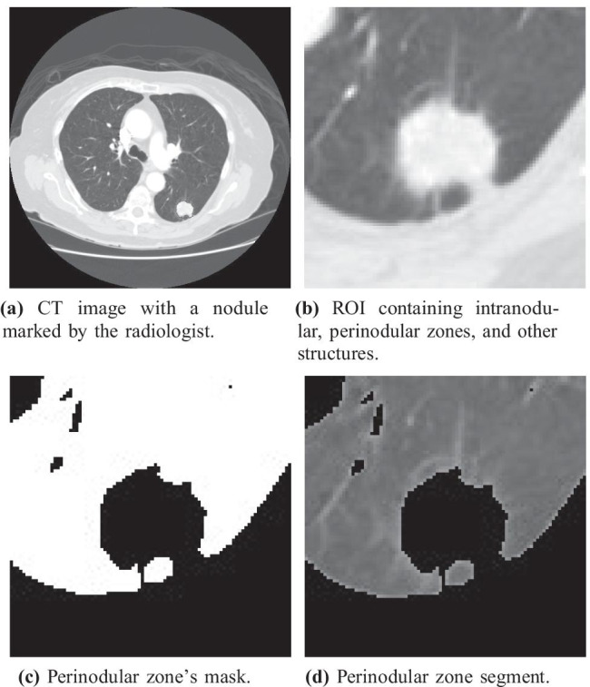
Process used for perinodular zone segmentation
A thoracic radiologist with 15+ years of experience validated the segmentation process. Due to the small differences in contrast between the final branches of the vessel trees and the parenchyma, it was not possible to remove them completely (Fig. 3). Based on the thoracic radiologist’s assessment, the segmentation algorithm was decided to be sufficiently good to be used to evaluate the parenchyma, with the exception of non-solid nodules. Therefore, the nodules labeled as non-solid by the annotations from the LIDC repository were excluded from this work.
Feature Extraction
To quantitatively assess the nodules’ morphological, textural aspects, and surroundings, we extracted 3D quantitative radiomic features from intranodular and perinodular zones. These features (n = 121) were divided into four traditional categories: First-Order Intensity, Second-Order Texture, Shape, and Margin Sharpness (Table 2).
Table 2.
Features extracted from I (intranodular) or P (perinodular) zones. 3D Margin Sharpness Features were extracted from both I and P
| Type | Details | Number |
|---|---|---|
| 3D Shape Features (I) | Compactness 1, Compactness 2, Spherical disproportion, | 9 |
| Sphericity, Area, Surface area, | ||
| Surface-volume ratio, Volume and Radium. | ||
| 3D Texture Features | Energy( = 0ž), Entropy( = 0ž), | 72 |
| (I) and (P) | Inverse difference moment( = 0ž), Shade( = 0ž), Inertia( = 0ž), | |
| Variance( = 0ž), Prominence( = 0ž), Correlation( = 0ž), | ||
| Homogeneity( = 0ž), Energy( = 45ž), Entropy( = 45ž), | ||
| Inverse difference moment( = 45ž), Shade( = 45ž), Inertia( = 45ž), | ||
| Variance( = 45ž), Prominence( = 45ž), Correlation( = 45ž), | ||
| Homogeneity( = 45ž), Energy( = 90ž), Entropy(ž = 90ž), | ||
| Inverse difference moment( = 90ž), Shade( = 90ž), Inertia( = 90ž), | ||
| Variance(ž), Prominence( = 90ž), Correlation( = 90ž), | ||
| Homogeneity( = 90ž), Energy( = 135ž), Entropy( = 135ž), | ||
| Inverse difference moment( = 135ž), Shade( = 135ž), Inertia( = 135ž), | ||
| Variance( = 135ž), Prominence( = 135ž), Correlation( = 135ž), | ||
| and Homogeneity( = 135ž). | ||
| 3D Margin Sharpness Features | Difference of two ends, Sum of values, Sum of squares, | 12 |
| (I and P) | Sum of logs, Arithmetic mean, Geometric mean, | |
| Population variance, Sample variance, Standard deviation, | ||
| Kurtosis measure, Skewness measure and Second central measure. |
3D Intensity Features (IF). We extracted 28 IF, being 14 from the intranodular and 14 from the perinodular zones [25]. These attributes compose the information about the histogram of the voxels intensity values [25].
3D Shape Features (SF). These features mathematically represent the nodule’s geometric characteristics [6]. In this work, 9 SF were extracted from the intranodular zone.
3D Texture Features (TF). We extracted 72 TF, being 36 from intranodular and 36 from perinodular zones [21]. The TF were obtained from the use of a co-occurrence matrix, a second-order statistical technique, applied in 4 angular orientations (, , , and ) and distance between pixels equal to one.
3D Margin Sharpness Features (MSF). Following a model partially proposed by Xu et al. [41], we extracted 12 MSF from the intensities of transition between intranodular and perinodular zones (Fig. 4). Xu et al. [41] defined the calculation of these features in two characteristics: (1) measurements of difference in intensity between the pixels from intranodular and perinodular zones; and (2) measurements of pixel intensity transition over the edge of the nodule. Hence, these features were obtained by generating orthogonal lines at the edge of the nodule, where the pixel values contained in these lines were stored in an array of gray levels, then, this array was sorted in ascending order, and the statistical features were calculated based on its content.
Fig. 4.
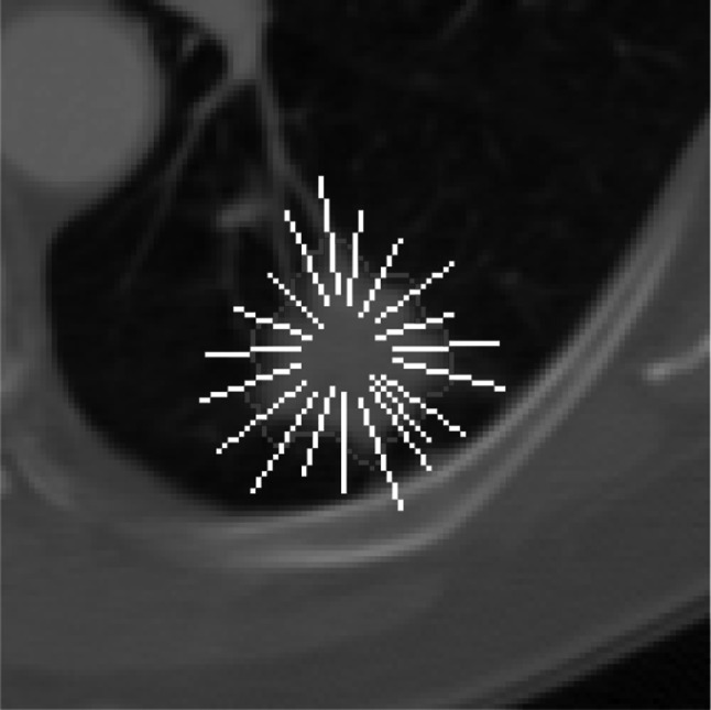
Orthogonal lines drawn over the edge of the pulmonary nodule
Three sets of data were created to evaluate the impact of the perinodular zone on the nodule classification:
The first set, identified as N, contains the attributes extracted only from the pulmonary nodule region;
The second set, , corresponds to the attributes from the N set plus the MSF;
The third set, , is the result of the addition of attributes from the perinodular zone.
These datasets were created to investigate the impact of adding attributes extracted from the perinodular zone on the classification process.
Feature Selection
In machine learning, the extraction and use of a large number of attributes are justified by the higher capacity for representation and the amount of information available for modeling. However, a large number of attributes also increases the likelihood of irrelevant attributes or feature noise, as well as increasing the chances of overfitting the classifier. The presence of these characteristics in a database leads to an increase in learning difficulties and loss of classification performance, especially for more sensitive models [31].
To select the most relevant attributes for the classification process and decreases the chances of overfitting, we have used the Genetic Algorithm (GA) on N, , and sets. GA is an optimization method widely used due to its efficiency in searching for an optimal (or near-optimal) solution [16, 24, 28, 42].
The GA uses techniques based on evolutionary biology concepts such as natural selection, heredity, mutation, and crossover. The functioning of the GA begins using the random generation of a population of individuals, where each individual is composed of a certain number of chromosomes. In the algorithm, each chromosome represents a feature set that needs to be optimized, usually having a binary value indicating whether the feature should be maintained (1) or not (0).
In the context of our work, the GA was deployed to optimize the area under the receiver operating characteristic curve (AUC-ROC). The population was composed of 50 individuals, but only the best four individuals of each generation were selected to compose each new generation through a uniform crossover with a 60% rate and a probability of mutation of 5%. The stopping criterion was a maximum of 100 generations or 10 generations without changing the best individual.
Classification
A total of fifteen classification models were built using the six machine learning algorithms with different hyperparameters: Decision Tree (DT), K-Nearest Neighbors (KNN), Logistic Regression (LR), Random Forest (RF) Support Vectors Machine (SVM), and XGBoost.
Two KNN models with distance-based weights were evaluated using different configurations: and . Three models with RF were analyzed using 100, 500, and 1000 random trees each, and division criteria entropy. With the SVM, three models with different kernels were evaluated: linear, Radial Basis Function (RBF) and polynomial; and, the XGBoost algorithm, we built five models using different numbers of trees: 15, 18, 20, 25, and 50; the DT model used the division criteria entropy, with best division as split strategy; and, the LR model was configured with liblinear solver and l2 penalty norm.
Each of the three data sets (N, , ) was applied to each model, which had their input attributes individually selected by the genetic algorithm.
In order to evaluate the predictive performance of the models, a 10-fold cross-validation with five repetitions was performed. Each fold was generated in a stratified way, therefore, replicating the original benign/malignant proportion of the dataset. Hence, each generated fold was composed of approximately 89 nodules, of which 61 were marked as benign and 28 as malignant.
During the cross-validation training stage, the SMOTE (Synthetic Minority Over-sampling Technique) technique was applied to generate synthetic nodule samples to obtain a balanced training set. This technique was chosen based on the results obtained from preliminary tests. In each step of the cross-validation, 9 folds were selected to compose the training set, and the remaining fold was used to compose the test set, maintaining the proper proportions. The sets used for training were composed of approximately 550 benign nodules and 252 malignant nodules. After applying the SMOTE algorithm, we generated approximately 298 synthetic samples per step to represent the malignant nodules. Therefore, we obtained a balanced training set with approximately 1,100 nodules (550 benign, 550 malignant) for each step of the cross-validation.
Metrics and Evaluation
We evaluated the performance of the classification models by taking the mean result from the five 10-fold cross-validations. The following six statistical metrics were performed: sensitivity (Eq. 1), specificity (Eq. 2), accuracy (Eq. 3), precision (Eq. 4), F1-score (Eq. 6), and AUC-ROC.
| 1 |
| 2 |
| 3 |
| 4 |
| 5 |
| 6 |
where TP is the number of true-positive samples, FN is the number of false-negative samples, TN is the number of true-negative samples, FP is the number of false-positive samples.
In the tree-based models, the attributes were evaluated according to the Gini importance [30]. We also used the frequency of occurrence of an attribute in the selection process as indicative of its relevance. Therefore, to evaluate the attributes, we analyzed its occurrence after the selection process in the best-evaluated configuration of each algorithm used to generate the predictive models.
To assess the statistical significance of the difference in performance obtained by the sets of attributes tested, we opted for the use of the Mann–Whitney Wilcoxon Rank-Sum test. In the comparison of two populations of performance sets, a p-value indicates that this difference has statistical significance.
The experiments were performed on a computer equipped with an Intel Core i5 CPU and 8GB of RAM, running the Ubuntu GNU/Linux operating system (version 18.04 LTS) and Python (version 3.7.3).
Results
This section presents the results obtained by our classification models. Initially, we compared the overall performance between each one of our datasets, and then we analyzed our best-evaluated model individually. Finally, we analyzed the most relevant features obtained by the selection process.
Table 3 presents the mean and standard deviation of the classification results obtained by the cross-validations for each machine learning model and the overall mean of these results for each feature set. The best overall performance was obtained with the N+M+P set. The overall mean AUC per feature set was also higher for the N+M+P set than for the others sets in all cases. The overall mean AUC for the N+M+P set was 0.901 ± 0.032, which is 0.008 higher than the same metric in the N set and 0.006 higher than that of the N+B set. In fact, a hypothesis test applied to these results proves the statistical significance of the improvement obtained when using the N+M+P set in the characterization of nodule when compared with the N+M and the N set () for all metrics with exception of sensitivity in the N+M set (). On the other hand, the hypothesis test was inconclusive () when we compared the relationship between the sets N+M and N for all metrics evaluated.
Table 3.
Mean and standard deviation of each metric after 5 repetitions of 10-fold cross-validation for each classification model
| Feature set | Model | Accuracy | F1 | PPV | Sensitivity | Specificity | AUC |
|---|---|---|---|---|---|---|---|
| N+M+P | DT | 80.24 ± 3.20 | 85.32 ± 2.48 | 87.13 ± 3.32 | 83.76 ± 4.21 | 72.53 ± 8.19 | 0.781 ± 0.040 |
| KNN-10 | 80.95 ± 4.77 | 84.92 ± 4.01 | 92.63 ± 3.66 | 78.56 ± 5.51 | 86.19 ± 7.04 | 0.909 ± 0.034 | |
| KNN-20 | 80.31 ± 3.94 | 84.15 ± 3.45 | 93.71 ± 3.09 | 76.52 ± 5.05 | 88.60 ± 5.76 | 0.910 ± 0.033 | |
| LR | 83.38 ± 3.62 | 87.21 ± 2.95 | 92.35 ± 3.53 | 82.79 ± 4.53 | 84.69 ± 7.36 | 0.912 ± 0.033 | |
| RF-100 | 83.26 ± 2.97 | 87.51 ± 2.33 | 89.71 ± 3.20 | 85.58 ± 4.03 | 78.15 ± 7.69 | 0.913 ± 0.028 | |
| RF-500 | 83.48 ± 3.25 | 87.67 ± 2.54 | 89.89 ± 3.22 | 85.71 ± 4.17 | 78.58 ± 7.46 | 0.915 ± 0.029 | |
| RF-1000 | 83.17 ± 3.39 | 87.35 ± 2.75 | 90.06 ± 3.13 | 85.00 ± 4.78 | 79.14 ± 7.23 | 0.914 ± 0.027 | |
| SVM-Linear | 83.28 ± 3.54 | 87.24 ± 2.83 | 91.50 ± 3.10 | 83.47 ± 4.09 | 82.84 ± 6.66 | 0.911 ± 0.033 | |
| SVM-Poly | 83.86 ± 3.45 | 88.10 ± 2.66 | 89.13 ± 3.49 | 87.34 ± 4.80 | 76.23 ± 8.81 | 0.903 ± 0.033 | |
| SVM-RBF | 84.26 ± 3.46 | 88.01 ± 2.80 | 92.07 ± 3.06 | 84.45 ± 4.48 | 83.84 ± 6.60 | 0.916 ± 0.031 | |
| XGBoost-15 | 81.58 ± 3.62 | 85.78 ± 2.97 | 91.16 ± 3.39 | 81.17 ± 4.55 | 82.50 ± 7.15 | 0.904 ± 0.031 | |
| XGBoost-18 | 81.65 ± 3.47 | 85.83 ± 2.92 | 91.19 ± 3.51 | 81.30 ± 4.96 | 82.43 ± 7.72 | 0.906 ± 0.031 | |
| XGBoost-20 | 81.54 ± 3.83 | 85.68 ± 3.21 | 91.34 ± 3.15 | 80.87 ± 5.11 | 82.99 ± 6.63 | 0.907 ± 0.032 | |
| XGBoost-25 | 81.94 ± 3.42 | 86.04 ± 2.86 | 91.48 ± 3.09 | 81.39 ± 4.76 | 83.14 ± 6.73 | 0.908 ± 0.030 | |
| XGBoost-50 | 82.47 ± 3.47 | 86.58 ± 2.82 | 91.20 ± 3.24 | 82.56 ± 4.45 | 82.29 ± 7.09 | 0.911 ± 0.030 | |
| Mean | 82.36 ± 3.56 | 86.49 ± 2.91 | 90.97 ± 3.28 | 82.70 ± 4.63 | 81.61 ± 7.21 | 0.901 ± 0.032 | |
| N+M | DT | 78.99 ± 4.00 | 84.35 ± 3.02 | 86.42 ± 3.73 | 82.52 ± 4.22 | 71.25 ± 8.99 | 0.769 ± 0.049 |
| KNN-10 | 80.74 ± 3.56 | 84.64 ± 3.23 | 93.16 ± 2.80 | 77.73 ± 5.01 | 87.32 ± 5.45 | 0.906 ± 0.030 | |
| KNN-20 | 80.39 ± 4.16 | 84.39 ± 3.62 | 92.78 ± 3.45 | 77.59 ± 5.37 | 86.54 ± 6.81 | 0.907 ± 0.035 | |
| LR | 82.16 ± 4.39 | 86.15 ± 3.71 | 91.80 ± 3.25 | 81.35 ± 5.73 | 83.92 ± 6.75 | 0.907 ± 0.033 | |
| RF-100 | 82.79 ± 3.30 | 87.22 ± 2.58 | 88.97 ± 3.22 | 85.72 ± 4.31 | 76.38 ± 7.82 | 0.909 ± 0.029 | |
| RF-500 | 83.06 ± 3.40 | 87.33 ± 2.74 | 89.59 ± 3.12 | 85.39 ± 4.91 | 77.95 ± 7.50 | 0.911 ± 0.028 | |
| RF-1000 | 82.77 ± 3.34 | 87.10 ± 2.66 | 89.55 ± 3.42 | 85.00 ± 4.74 | 77.87 ± 8.04 | 0.911 ± 0.029 | |
| SVM-Linear | 81.76 ± 3.96 | 85.81 ± 3.35 | 91.77 ± 3.21 | 80.77 ± 5.24 | 83.92 ± 6.71 | 0.905 ± 0.032 | |
| SVM-Poly | 80.93 ± 3.64 | 87.22 ± 2.15 | 81.23 ± 4.17 | 94.48 ± 3.65 | 51.24 ± 14.23 | 0.900 ± 0.032 | |
| SVM-RBF | 82.50 ± 3.78 | 86.71 ± 3.07 | 90.42 ± 3.34 | 83.47 ± 4.76 | 80.35 ± 7.53 | 0.908 ± 0.031 | |
| XGBoost-15 | 80.55 ± 3.85 | 84.94 ± 3.32 | 90.39 ± 3.25 | 80.35 ± 5.59 | 81.00 ± 6.92 | 0.897 ± 0.031 | |
| XGBoost-18 | 80.62 ± 3.66 | 84.99 ± 3.10 | 90.58 ± 3.57 | 80.29 ± 5.19 | 81.35 ± 7.64 | 0.898 ± 0.030 | |
| XGBoost-20 | 80.49 ± 3.94 | 84.87 ± 3.36 | 90.50 ± 3.47 | 80.12 ± 5.36 | 81.28 ± 7.31 | 0.898 ± 0.031 | |
| XGBoost-25 | 80.93 ± 3.72 | 85.28 ± 3.23 | 90.46 ± 3.42 | 80.94 ± 5.63 | 80.94 ± 7.69 | 0.897 ± 0.031 | |
| XGBoost-50 | 81.16 ± 3.32 | 85.59 ± 2.72 | 90.06 ± 3.49 | 81.75 ± 4.53 | 79.87 ± 7.87 | 0.902 ± 0.029 | |
| Mean | 81.32 ± 3.73 | 85.77 ± 3.06 | 89.85 ± 3.39 | 82.50 ± 4.95 | 78.75 ± 7.82 | 0.895 ± 0.032 | |
| N | DT | 79.29 ± 4.02 | 84.49 ± 3.29 | 86.78 ± 3.42 | 82.60 ± 5.81 | 72.02 ± 8.72 | 0.773 ± 0.044 |
| KNN-10 | 80.99 ± 4.17 | 84.96 ± 3.68 | 92.55 ± 3.01 | 78.72 ± 5.56 | 85.97 ± 5.87 | 0.901 ± 0.030 | |
| KNN-20 | 79.70 ± 4.15 | 83.79 ± 3.76 | 92.31 ± 3.39 | 76.97 ± 5.84 | 85.69 ± 6.74 | 0.905 ± 0.033 | |
| LR | 81.49 ± 4.08 | 85.49 ± 3.53 | 92.19 ± 3.42 | 79.93 ± 5.66 | 84.90 ± 6.92 | 0.904 ± 0.032 | |
| RF-100 | 83.30 ± 3.26 | 87.60 ± 2.55 | 89.34 ± 3.44 | 86.13 ± 4.54 | 77.09 ± 8.48 | 0.905 ± 0.027 | |
| RF-500 | 82.99 ± 3.47 | 87.35 ± 2.70 | 89.23 ± 3.48 | 85.74 ± 4.52 | 76.95 ± 8.47 | 0.908 ± 0.028 | |
| RF-1000 | 82.83 ± 3.00 | 87.14 ± 2.45 | 89.62 ± 3.24 | 85.03 ± 4.76 | 78.00 ± 7.96 | 0.907 ± 0.028 | |
| SVM-Linear | 81.15 ± 3.60 | 85.27 ± 3.14 | 91.72 ± 3.00 | 79.86 ± 5.08 | 83.98 ± 6.23 | 0.904 ± 0.032 | |
| SVM-Poly | 82.27 ± 3.25 | 87.37 ± 2.32 | 85.73 ± 3.91 | 89.35 ± 4.42 | 66.76 ± 10.86 | 0.890 ± 0.038 | |
| SVM-RBF | 83.18 ± 3.59 | 87.14 ± 2.95 | 91.52 ± 3.10 | 83.34 ± 4.77 | 82.84 ± 6.71 | 0.906 ± 0.028 | |
| XGBoost-15 | 79.53 ± 3.60 | 83.99 ± 3.17 | 90.46 ± 3.46 | 78.67 ± 5.61 | 81.42 ± 7.52 | 0.898 ± 0.032 | |
| XGBoost-18 | 80.62 ± 3.62 | 85.02 ± 3.05 | 90.43 ± 3.60 | 80.48 ± 5.30 | 80.93 ± 7.87 | 0.898 ± 0.032 | |
| XGBoost-20 | 79.88 ± 3.49 | 84.26 ± 3.10 | 90.80 ± 3.32 | 78.86 ± 5.48 | 82.13 ± 7.22 | 0.900 ± 0.031 | |
| XGBoost-25 | 81.14 ± 3.40 | 85.48 ± 2.96 | 90.44 ± 3.49 | 81.33 ± 5.45 | 80.72 ± 7.94 | 0.899 ± 0.031 | |
| XGBoost-50 | 81.58 ± 3.34 | 85.89 ± 2.77 | 90.47 ± 3.31 | 81.94 ± 4.63 | 80.79 ± 7.38 | 0.900 ± 0.030 | |
| Mean | 81.33 ± 3.60 | 85.68 ± 3.03 | 90.24 ± 3.37 | 81.93 ± 5.16 | 80.01 ± 7.66 | 0.893 ± 0.032 |
When we consider the AUC, the best-evaluated model with the N+M+P set was the one using the SVM algorithm with RBF kernel, which obtained a mean AUC of 0.916 ± 0.031 (Fig. 5). This same model, using the N+M set, obtained a mean AUC of 0.908 ± 0.031, while the N set yielded an AUC of 0.906 ± 0.028. The number of selected features for the SVM-RBF model in sets N+M+P, N+M, and N was, respectively, 30, 13, and 14. Table 4 presents those features grouped by type and region of extraction. The hypothesis test applied to the results obtained by this model showed statistical significance in the relation between the sets N+M+P and N (). The relation between the sets N+M+P and N+M, N+M and N was inconclusive ( and , respectively).
Fig. 5.
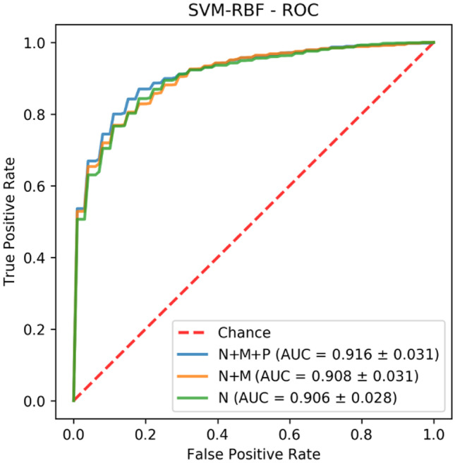
ROC curve of SVM-RBF model
Table 4.
Selected features of SVM-RBF model for each evaluated set
| Region | Type | N | N+M | N+M+P |
|---|---|---|---|---|
| Nodule | IF | Entropy | Maximum intensity | Entropy |
| Maximum intensity | Maximum intensity | |||
| Medium intensity | Means absolute | |||
| Range | Mean square root | |||
| Skewness | Medium intensity | |||
| Range | ||||
| Skewness | ||||
| Standard deviation | ||||
| TF | Correlation 45ž | Correlation 0ž | Prominence 45ž and 90ž | |
| Prominence 0ž, 45ž, 90ž and 135ž | Entropy 135ž | Shade 45ž, 90ž and 135ž | ||
| Shade 0ž | Homogeneity 0ž and 135ž | Variance 45ž and 135ž | ||
| IDM 0ž, 45ž, 90ž and 135ž | ||||
| SF | Spherical disproportion | Spherical disproportion | Area | |
| Sphericity | Sphericity | Spherical disproportion | ||
| Surface-volume ratio | Surface-volume ratio | Sphericity | ||
| Margin | MSF | NA | Skewness | Arithmetic Mean |
| Skewness | ||||
| Parenchyma | IF | NA | NA | Meridian Intensity |
| Skewness | ||||
| F | NA | NA | Inverse difference moment 135ž | |
| Prominence 45ž, 90ž and 135ž | ||||
| Shade 90ž and 135ž | ||||
| Variance 90ž |
IF Intensity Features; TF Texture Features; SF Shape Features; MSF Margin Sharpness Features; NA Not Applied
The frequency of occurrence of an attribute in the selection process was used as an indication of its importance. For each model evaluated, and more specifically for those that used the same machine learning algorithms, we took into consideration only those with the best result, considering the AUC; however, results from the Decision Tree model were not considered due to its poor performance. The results presented below refer to the SVM-RBF, RF-500, KNN-20, LR, and XGBoost-50 models with N+M+P set. Features that have been used in more than half of these five models were considered the most relevant (Frequency >= 3).
- Frequency 5
- Nodule-originated features: shade in 45ž;
- Margin-originated features: skewness;
- Frequency 4
- Nodule-originated features: maximum and mean intensity, spherical disproportion;
- Margin-originated features: sum of squares;
- Parenchyma-originated features: skewness, prominence in 135ž;
- Frequency 3
- Nodule-originated features: entropy, uniformity, entropy in 0ž, homogeneity in 0 and 45ž, correlation in 90 and 135ž, diameter, compactness 2, prominence in 45 and 90ž, sphericity;
- Margin-originated features: second central measure;
- Parenchyma-originated features: energy, entropy, correlation in 90ž, energy in 135ž, shade in 90ž and 135ž
For the best-evaluated tree-based models, such as XGBoost and Random Forest, we calculated the Gini importance and used it as a metric of feature importance. Fig. 6 shows the 20 most important selected features, considering models RF-500 and XGBoost-50 with the N+M+P set. This feature relevance ranking is an indication of how much the perinodular features have influenced the classification process. Our results showed that 6 of the 20 most important features were originated from the perinodular region (Fig. 6a), while in Fig. 6b the number of perinodular features is 8. This occurrence of these features within the top 20 most important features indicates, by itself, some relevance of the perinodular region to the classification process. Moreover, both graphs showed the high importance of shape features, like diameter, volume, and spherical disproportion. Features like parenchymal energy and margin sharpness skewness also presented high importance in both tree-based models.
Fig. 6.

Gini Importance of the 20 best features of the RF-500 and XGBoost-50 models with N+M+P set. *_N = Nodule-originated feature. *_M = Margin-originated feature. *_P = Parenchyma-originated feature. SD = Spherical Disproportion. IDM = Inverse Difference Moment. PV = Population Variance
Related works
Felix et al. [16] proposed a model for classification of small nodules, 3-10mm, combining nodule texture and margin sharpness features. The dataset used in the predictive model contained 274 pulmonary nodules (137 malignant, 137 benign). Its classifier model used the Multilayer Perceptron algorithm with a set of 26 selected features and obtained an average AUC of 0.820.
Ferreira et al. [17] proposed a pulmonary nodule classification model using a set of 48 features composed of texture and margin sharpness descriptors. Different classifiers were evaluated, and the best result was obtained using the Random Forest algorithm with all 48 features, which achieved an average AUC of 0.856 in a set of 600 pulmonary nodules (300 malignant, 300 benign).
Dhara et al. [14] proposed a classification scheme of pulmonary nodules combining shape-based, margin-based, and texture-based features. In all, 56 features were used to characterize 891 pulmonary nodules in 3 configurations of datasets based on the malignancy level. The classification was performed with a Support Vectors Machine algorithm, and the best-evaluated dataset obtained an average AUC of 0.950.
Beig et al. [10] combined perinodular and intranodular features to generate a classification model to distinguish non-small cell lung adenocarcinomas from granulomas on CT images. Nodule shape, wavelet, and texture-based features were extracted from a set of 290 CT lung nodules, which 145 were used to training and 145 to test. A support vectors machine with linear kernel was used as the classifier. The combined perinodular and intranodular features yielded an AUC of 0.800, achieving higher performance than with only intranodular features (AUC of 0.750).
Dilger et al. [15] used a set of 358 radiomic features (including features from nodule, parenchyma, and global lung measurements) of 50 samples in a study of nodule classification. The study aimed to investigate the performance in the classification of lung nodules by using radiomic features from the parenchyma. Its predictive model with the nodule and parenchyma features obtained an average AUC of 0.938, 0.200 higher than the model composed only with nodule features. Their findings indicated that the presence of these features positively influences the performance of the classification. However, due to the low number of available samples, the statistical significance of their results could not be verified.
Uthoff et al. [36] conducted a study on the effects of including the lung parenchyma in the classification process. A set of 363 lung nodules (74 malignant, 289 benign) was used to train the predictive model, and a set with 100 nodules (50 malignant, 50 benign) was used to validate the model exclusively. A comparative analysis of the model’s performance was performed by adding several quantities of the parenchyma. Its results indicated that the size of the included parenchyma that optimizes the gain of information on the nature of the tumor is 75% of the nodule diameter. The average AUC obtained by the model evaluated in the independent set was 0.965, proven to be statistically significant.
Discussion
The results presented in Table 3, specifically the three lines highlighting the mean of each metrics, confirm the relevance of the perinodular region for medical image characterization. This region information when associated with the information of the intranodular region yielded overall mean AUC-ROC superior to the other characterization approaches. These results corroborate those already presented by Uthoff, Dilger, and Beig et al. [10, 15, 36], indicating performance improvement with the use of the datasets that include features from the perinodular zone. Although other studies did not use the same set of features as we did, and therefore not all significant features could be matched with our findings. Our set of relevant features had intersections with significant features obtained in the studies of Dilger (nodule mean intensity, sphericity, diameter, and parenchyma entropy), and Uthoff (nodule entropy, sphericity, and diameter).
When analyzing the nature of a pulmonary nodule, some features tend to be more associated with a malignant lesion than a benign one. Several categories of features can be related to the malignancy potential of a nodule. Factors such as texture heterogeneity may reflect changes in the tumor region caused by the presence of neoplastic tissues in the nodule, such as cell infiltration, abnormal angiogenesis, myxoid changes, and necrosis [9, 12, 20]. Morphological changes in the nodule, such as spiculation, caused by obstruction of pulmonary vessels or lymphatic channels filled with tumor cells, are also linked to a greater likelihood of malignancy, as benign nodules tend to be more spherical in shape and smooth [16, 35]. These factors could explain some of our findings, such as highly relevant morphological and shape features as sphericity, spherical disproportion, and diameter. Our most relevant margin feature, skewness, is a measure of asymmetry related to the differentiation of the more symmetric behavior of benign nodule as malignant nodule tends to be more chaotic. We also found skewness as an important feature of the parenchymal region, together with entropy, energy, and other textural measurements, which could indicate that the subtle changes in this region are important to the accurate differentiation of benign and malignant nodule.
Although recent relevant studies in pulmonary nodule classification have focused on the use of deep learning models, the use of models based on radiomic attributes allows us to have greater control and interpretability of the results obtained. Above all, the use of radiomic attributes in this work allowed us to analyze relevant characteristics for the differentiation of pulmonary nodules, evaluate the impact caused by the addition of the perinodular zone in the classification process, and ratify the findings of related works that adopted similar methodologies.
While similar works have already assessed the impact of perinodular features in nodule classification, they were conducted on private datasets, making them difficult to reproduce, whereas this study was conducted on a publicly available dataset (i.e., LIDC image repository [7]). Compared to other studies from literature, we used a larger dataset, and we were able to verify the statistical relevance of the results. We also specifically assessed the features that most influenced the classification process, which is important for clinical purposes, allowing the reproducibility of the models.
However, our work had some limitations. First, the ROI used in the perinodular zone segmentation algorithm was defined with a fixed size (2x the nodule’s size), and we included only solid nodules in this work. Therefore, it is necessary to evaluate in future works how the ROI’s size affects the perinodular zone segmentation algorithm, and if this implies an improvement in the pulmonary nodule classification process and include a more diversified nodule dataset. Also, as the goal was to evaluate the parenchyma and the nodule’s margin, we excluded some important structures, e. g. pleural tags and vessels, which could be additional indicators of malignancy [22, 38]. That said, in future works, we would add more features to characterize the nodule surrounding structures and better assess their effects on nodule classification. The sizes of our nodules were not balanced to maintain a similar size for both benign and malignant nodules. Therefore, the malignant nodules were, on average, significantly larger than the average size of the benign nodules, which may explain the high importance of the diameter attribute in Fig. 6. Although this appears to be the behavior of lung nodules in real-world applications, therefore, the results obtained in this study may be more general than studies that use a dataset in which nodules sizes are balanced between its classes.
Conclusion
This paper presented an assessment of the impact of including the perinodular zone in solid lung nodule characterization and further classification of malignancy likelihood. Motivated by reproducible research, we used a large public dataset of lung nodule images and extracted fine-tuned radiomic attributes from the perinodular and intranodular zones, as well as attributes from the nodules’ margin sharpness. The combination of attributes from the perinodular and intranodular zones in the image characterization resulted in an improvement in all the metrics analyzed when compared to intranodular-only characterization (p<0.05).
The SVM-RBF algorithm with the N+M+P set yielded the highest classification performance, achieving an average of 0.916 (AUC-ROC), representing an increase in the AUC when we analyzed only the intranodular zone (0.906 AUC-ROC). Moreover, the results showed the high importance rate of the perinodular attributes, which occupied six positions in the list of the 20 most important attributes in the best-evaluated tree-based model, with the Random Forest algorithm. Therefore, our results highlighted the importance of using the perinodular zone in the classification process of solid pulmonary nodules.
Declarations
Conflicts of interest
On behalf of all authors, the corresponding author states that there is no conflict of interest.
Footnotes
Publisher’s Note
Springer Nature remains neutral with regard to jurisdictional claims in published maps and institutional affiliations.
Contributor Information
José Lucas Leite Calheiros, Email: lucaslc@uc.ufal.br.
Lucas Benevides Viana de Amorim, Email: lucas@ic.ufal.br.
Lucas Lins de Lima, Email: lll@ic.ufal.br.
Ailton Felix de Lima Filho, Email: afdlf2@gmail.com.
José Raniery Ferreira Júnior, Email: jose.raniery@alumni.usp.br.
Marcelo Costa de Oliveira, Email: oliveiramc@ic.ufal.br.
References
- 1.Siegel RL, Miller KD, Jemal A: Cancer statistics, 2020. CA: A Cancer Journal for Clinicians 70(1), 7–30 (2020). https://acsjournals.onlinelibrary.wiley.com/doi/abs/10.3322/caac.21590 [DOI] [PubMed]
- 2.Bray F, Ferlay J, Soerjomataram I, Siegel RL, Torre LA, Jemal A: Global cancer statistics 2018: Globocan estimates of incidence and mortality worldwide for 36 cancers in 185 countries. CA: A Cancer Journal for Clinicians 68(6), 394–424 (2018). https://acsjournals.onlinelibrary.wiley.com/doi/abs/10.3322/caac.21492 [DOI] [PubMed]
- 3.Huang P, Park S, Yan R, Lee J, Chu LC, Lin CT, Hussien A, Rathmell J, Thomas B, Chen C, HalS R, Ettinger DS, Brock M, Hu P, Fishman EK, Gabrielson E, Lam S. Added value of computer-aided CT image features for early lung cancer diagnosis with small pulmonary nodules: A matched case-control study. Radiology. 2018;286(1):286–295. doi: 10.1148/radiol.2017162725. [DOI] [PMC free article] [PubMed] [Google Scholar]
- 4.Nishi SP, Zhou J, Okereke I, Kuo YF, Goodwin J. Use of imaging and diagnostic procedures after low-dose ct screening for lung cancer. Chest. 2020;157(2):427–434. doi: 10.1016/j.chest.2019.08.2187. [DOI] [PMC free article] [PubMed] [Google Scholar]
- 5.Schreuder A, van Ginneken B, Scholten ET, Jacobs C, Prokop M, Sverzellati N, Desai SR, Devaraj A, Schaefer-Prokop CM. Classification of ct pulmonary opacities as perifissural nodules: Reader variability. Radiology. 2018;288(3):867–875. doi: 10.1148/radiol.2018172771. [DOI] [PubMed] [Google Scholar]
- 6.Aerts H, et al. Decoding tumour phenotype by noninvasive imaging using a quantitative radiomics approach. Nature communications. 2014;5:4006. doi: 10.1038/ncomms5006. [DOI] [PMC free article] [PubMed] [Google Scholar]
- 7.Armato SG, et al. The lung image database consortium (LIDC) and image database resource initiative (IDRI): a completed reference database of lung nodules on CT scans. Medical physics. 2011;38(2):915–931. doi: 10.1118/1.3528204. [DOI] [PMC free article] [PubMed] [Google Scholar]
- 8.Bartholmai B, et al. Pulmonary Nodule Characterization, Including Computer Analysis and Quantitative Features. Journal of Thoracic Imaging. 2015;30(2):139–156. doi: 10.1097/RTI.0000000000000137. [DOI] [PubMed] [Google Scholar]
- 9.Bayanati H, Thornhill ER, Souza CA, Sethi-Virmani V, Gupta A, Maziak D, Amjadi K, Dennie C: Quantitative CT texture and shape analysis: Can it differentiate benign and malignant mediastinal lymph nodes in patients with primary lung cancer? European Radiology 25(2), 480–487 (2015). 10.1007/s00330-014-3420-6 [DOI] [PubMed]
- 10.Beig N, Khorrami M, Alilou M, Prasanna P, Braman N, Orooji M, Rakshit S, Bera K, Rajiah P, Ginsberg J, Donatelli C, Thawani R, Yang M, Jacono F, Tiwari P, Velcheti V, Gilkeson R, Linden P, Madabhushi A. Perinodular and intranodular radiomic features on lung ct images distinguish adenocarcinomas from granulomas. Radiology. 2019;290(3):783–792. doi: 10.1148/radiol.2018180910. [DOI] [PMC free article] [PubMed] [Google Scholar]
- 11.Choy G, Khalilzadeh O, Michalski M, Do S, Samir AE, Pianykh OS, Geis JR, Pandharipande, PV, Brink JA, Dreyer KJ: Current applications and future impact of machine learning in radiology. Radiology 288(2), 318–328 (2018). 10.1148/radiol.2018171820. https://pubmed.ncbi.nlm.nih.gov/29944078 [DOI] [PMC free article] [PubMed]
- 12.Davnall F, Yip CS, Ljungqvist G, Selmi M, Ng F, Sanghera B, Ganeshan B, Miles KA, Cook GJ, Goh V: Assessment of tumor heterogeneity: An emerging imaging tool for clinical practice? (2012). 10.1007/s13244-012-0196-6. https://insightsimaging.springeropen.com/articles/10.1007/s13244-012-0196-6 [DOI] [PMC free article] [PubMed]
- 13.Degnan AJ, Ghobadi EH, Hardy P, Krupinski E, Scali EP, Stratchko L, Ulano A, Walker E, Wasnik AP, Auffermann WF. Perceptual and interpretive error in diagnostic radiology-causes and potential solutions. Academic radiology. 2019;26(6):833–845. doi: 10.1016/j.acra.2018.11.006. [DOI] [PubMed] [Google Scholar]
- 14.Dhara AK, Mukhopadhyay S, Dutta A, Garg M, Khandelwal N. A Combination of Shape and Texture Features for Classification of Pulmonary Nodules in Lung CT Images. Journal of Digital Imaging. 2016;29(4):466–475. doi: 10.1007/s10278-015-9857-6. [DOI] [PMC free article] [PubMed] [Google Scholar]
- 15.Dilger SKN, Uthoff J, Judisch A, Hammond E, Mott SL, Smith BJ, Newell JDJ, Hoffman EA, Sieren JC: Improved pulmonary nodule classification utilizing quantitative lung parenchyma features. pp. 041,004–041,004. Society of Photo-Optical Instrumentation Engineers (2015). 10.1117/1.JMI.2.4.041004. https://pubmed.ncbi.nlm.nih.gov/26870744 [DOI] [PMC free article] [PubMed]
- 16.Felix A, Oliveira M, Machado A, Raniery J: Using 3d texture and margin sharpness features on classification of small pulmonary nodules. In: 2016 29th SIBGRAPI Conference on Graphics, Patterns and Images (SIBGRAPI), pp. 394–400 (2016)
- 17.Ferreira JRJ, Oliveira MC, de Azevedo-Marques PM: Characterization of pulmonary nodules based on features of margin sharpness and texture. J Digit Imaging 31(4), 451–463 (2018). 10.1007/s10278-017-0029-8. https://pubmed.ncbi.nlm.nih.gov/29047033 [DOI] [PMC free article] [PubMed]
- 18.Ferreira-Junior JR, Koenigkam-Santos M, Tenorio APM, Faleiros MC, Cipriano FEG, Fabro AT, Nappi J, Yoshida H, de Azevedo-Marques PM. Ct-based radiomics for prediction of histologic subtype and metastatic disease in primary malignant lung neoplasms. International journal of computer assisted radiology and surgery. 2020;15(1):163–172. doi: 10.1007/s11548-019-02093-y. [DOI] [PubMed] [Google Scholar]
- 19.Firmino M, Angelo G, Morais H, Dantas MR, Valentim R: Computer-aided detection (cade) and diagnosis (cadx) system for lung cancer with likelihood of malignancy. BioMedical Engineering OnLine 15(1), 2–17 (2016). 10.1186/s12938-015-0120-7. 10.1186/s12938-015-0120-7 [DOI] [PMC free article] [PubMed]
- 20.Ganeshan B, Panayiotou E, Burnand K, Dizdarevic S, Miles K. Tumour heterogeneity in non-small cell lung carcinoma assessed by CT texture analysis: A potential marker of survival. European Radiology. 2012;22(4):796–802. doi: 10.1007/s00330-011-2319-8. [DOI] [PubMed] [Google Scholar]
- 21.Haralick RM, Shanmugam K, Dinstein I: Textural features for image classification. IEEE Transactions on Systems, Man, and Cybernetics SMC-3(6), 610–621 (1973). 10.1109/TSMC.1973.4309314 [DOI]
- 22.Hsu JS, Han IT, Tsai TH, Lin SF, Jaw TS, Liu GC, Chou SH, Chong IW, Chen CY: Pleural tags on ct scans to predict visceral pleural invasion of non-small cell lung cancer that does not abut the pleura. Radiology 279(2), 590–596 (2016). PMID: 26653684 10.1148/radiol.2015151120. [DOI] [PubMed]
- 23.Kai Huang L, J Iun M, Wangt J: Image thresholding by minimizing the measure of fuzziness. In: Pattern Recognition, 1995,28(1):41-51. 113 International Archives of the Photogrammetry, Remote Sensing and Spatial Information Sciences. Vol. XXXVII. Part B2. Beijing 2008 (1995).
- 24.Il-Seok Oh. Jin-Seon Lee, Byung-Ro Moon: Hybrid genetic algorithms for feature selection. IEEE Transactions on Pattern Analysis and Machine Intelligence. 2004;26(11):1424–1437. doi: 10.1109/TPAMI.2004.105. [DOI] [PubMed] [Google Scholar]
- 25.Judisch, A., Hoffman, E.A., Newell, J.D., Sieren, J.C.: The Use Of Surrounding Lung Parenchyma For The Automated Classification Of Pulmonary Nodules, pp. A5457–A5457. https://www.atsjournals.org/doi/abs/10.1164/ajrccm-conference.2013.187.1_MeetingAbstracts.A5457
- 26.Junior JRF, Oliveira MC, de Azevedo-Marques PM. Cloud-based nosql open database of pulmonary nodules for computer-aided lung cancer diagnosis and reproducible research. J Digit Imaging. 2016;29(6):716–729. doi: 10.1007/s10278-016-9894-9. [DOI] [PMC free article] [PubMed] [Google Scholar]
- 27.Kadir T, Gleeson F: Lung cancer prediction using machine learning and advanced imaging techniques. Translational lung cancer research 7(3), 304–312 (2018). https://pubmed.ncbi.nlm.nih.gov/30050768 [DOI] [PMC free article] [PubMed]
- 28.Leardi R, Boggia R, Terrile M: Genetic algorithms as a strategy for feature selection. J Chemom 6(5), 267–281 (1992). https://onlinelibrary.wiley.com/doi/abs/10.1002/cem.1180060506
- 29.Lima LL, Ferreira Junior JR, Oliveira MC: Toward classifying small lung nodules with hyperparameter optimization of convolutional neural networks. Comput Intell 1–20 (2020). https://onlinelibrary.wiley.com/doi/abs/10.1111/coin.12350
- 30.Nembrini S, Knig IR, Wright MN: The revival of the Gini importance? Bioinformatics 34(21), 3711–3718 (2018). 10.1093/bioinformatics/bty373 [DOI] [PMC free article] [PubMed]
- 31.Nettleton DF, Orriols-Puig A, Fornells A: A study of the effect of different types of noise on the precision of supervised learning techniques. Artif Intell Rev 33(4), 275–306 (2010). 10.1007/s10462-010-9156-z [DOI]
- 32.Nishio M, Sugiyama O, Yakami M, Ueno S, Kubo T, Kuroda T, Togashi K: Computer-aided diagnosis of lung nodule classification between benign nodule, primary lung cancer, and metastatic lung cancer at different image size using deep convolutional neural network with transfer learning. PloS one 13(7), e0200,721–e0200,721 (2018). https://pubmed.ncbi.nlm.nih.gov/30052644 [DOI] [PMC free article] [PubMed]
- 33.Pinsky PF, Gierada DS, Nath PH, Kazerooni E, Amorosa J. National lung screening trial: Variability in nodule detection rates in chest ct studies. Radiology. 2013;268(3):865–873. doi: 10.1148/radiol.13121530. [DOI] [PMC free article] [PubMed] [Google Scholar]
- 34.Shariaty F, Mousavi M: Application of cad systems for the automatic detection of lung nodules. Informatics in Medicine Unlocked 15, 100,173 (2019). http://www.sciencedirect.com/science/article/pii/S2352914818301382
- 35.Snoeckx A, Reyntiens P, Desbuquoit D, Spinhoven MJ, Van Schil PE, van Meerbeeck JP, Parizel PM: Evaluation of the solitary pulmonary nodule: size matters, but do not ignore the power of morphology (2018). 10.1007/s13244-017-0581-2 [DOI] [PMC free article] [PubMed]
- 36.Uthoff J, Stephens MJ, Newell Jr JD, Hoffman EA, Larson J, Koehn N, De Stefano FA, Lusk CM, Wenzlaff AS, Watza D, Neslund-Dudas C, Carr LL, Lynch DA, Schwartz A.G, Sieren JC: Machine learning approach for distinguishing malignant and benign lung nodules utilizing standardized perinodular parenchymal features from ct. Med Phys 46(7), 3207–3216 (2019). https://aapm.onlinelibrary.wiley.com/doi/abs/10.1002/mp.13592 [DOI] [PMC free article] [PubMed]
- 37.Van Riel, S., Jacobs, C., Scholten, E.: Observer variability for lung-rads categorisation of lung cancer screening cts: impact on patient management. Eur Radiol 29(1), 924–931 (2019) [DOI] [PMC free article] [PubMed]
- 38.Wang X, Leader JK, Wang R, Wilson D, Herman J, Yuan JM, Pu J: Vasculature surrounding a nodule: A novel lung cancer biomarker. Lung Cancer 114, 38–43 (2017). https://aapm.onlinelibrary.wiley.com/doi/abs/10.1002/mp.13592 [DOI] [PMC free article] [PubMed]
- 39.Wei G, Cao H, Ma H, Qi S, Qian W, Ma Z: Content-based image retrieval for lung nodule classification using texture features and learned distance metric. J Med Sys 42(1), 13 (2017). 10.1007/s10916-017-0874-5 [DOI] [PubMed]
- 40.Wormanns D, Hamer O: Glossary of terms for thoracic imaging–german version of the fleischner society recommendations. RoFo: Fortschritte auf dem Gebiete der Rontgenstrahlen und der Nuklearmedizin 187(8), 638–61 (2015) [DOI] [PubMed]
- 41.Xu J, et al. Quantifying the margin sharpness of lesions on radiological images for content-based image retrieval. Med Phys. 2012;39:5405–18. doi: 10.1118/1.4739507. [DOI] [PMC free article] [PubMed] [Google Scholar]
- 42.Yang, J., Honavar, V.: Feature Subset Selection Using a Genetic Algorithm, pp. 117–136. Springer US, Boston, MA (1998). 10.1007/978-1-4615-5725-88. URL 10.1007/978-1-4615-5725-8_8 [DOI]