Multi-level Kronecker Convolutional Neural Network (ML-KCNN) for Glioma Segmentation from Multi-modal MRI Volumetric Data

Abstract

The development of an automated glioma segmentation system from MRI volumes is a difficult task because of data imbalance problem. The ability of deep learning models to incorporate different layers for data representation assists medical experts like radiologists to recognize the condition of the patient and further make medical practices easier and automatic. State-of-the-art deep learning algorithms enable advancement in the medical image segmentation area, such a segmenting the volumes into sub-tumor classes. For this task, fully convolutional network (FCN)-based architectures are used to build end-to-end segmentation solutions. In this paper, we proposed a multi-level Kronecker convolutional neural network (MLKCNN) that captures information at different levels to have both local and global level contextual information. Our ML-KCNN uses Kronecker convolution, which overcomes the missing pixels problem by dilated convolution. Moreover, we used a post-processing technique to minimize false positive from segmented outputs, and the generalized dice loss (GDL) function handles the data-imbalance problem. Furthermore, the combination of connected component analysis (CCA) with conditional random fields (CRF) used as a post-processing technique achieves reduced Hausdorff distance (HD) score of 3.76 on enhancing tumor (ET), 4.88 on whole tumor (WT), and 5.85 on tumor core (TC). Dice similarity coefficient (DSC) of 0.74 on ET, 0.90 on WT, and 0.83 on TC. Qualitative and visual evaluation of our proposed method shown effectiveness of the proposed segmentation method can achieve performance that can compete with other brain tumor segmentation techniques.

Introduction

Automatic segmentation of tumorous regions from the brain is a difficult task because it involves a vast amount of data and contains artifacts due to limited acquisition time; the patient’s motion and soft tissue boundaries are not adequately defined. One of the reasons is the appearance of tumors in different shapes and sizes [1]. Segmentation of gliomas from medical resonance imaging (MRI) scans plays a crucial role during treatment, but it is a time-consuming process and requires expert supervision. Gliomas is a type of tumor that appears in the brain and spinal cord region. World Health Organization (WHO) classified brain tumors into four groups based on their grading scheme [1]. They categorized it into grades I–IV based on their aggressiveness [2]. Tumors of grade I and II are called low-grade gliomas (LGG) and III or IV are called high-grade gliomas (HGG). The standard non-invasive technique for the detection of brain tumors is MRI [3].

In clinical application, radiologists perform manual segmentation, which has an overwhelming burden, subjective and hard to accomplish repetitive segmentation. Self-automatic segmentation algorithms can segment region of interest (ROI) having the benefit of manual and automatic segmentation and improve segmentation efficiency. However, automatic segmentation is a difficult task.

However, applying the need of automated processing is difficult that requires initial seed points and iteration termination conditions, among others, whereas automatic segmentation algorithm does not require any human interaction and works automatically. Automatic segmentation algorithms enable to build end-to-end application for diagnosis of glioma. Building an automatic glioma segmentation system while improving the accuracy is a key challenge. Classical machine learning–based techniques consume a significant amount of time on feature extraction, whereas deep leaning–based system has the power to automatically extract features enabling to build end-to-end segmentation system. In terms of performance, machine learning (ML) architectures failed in reaching convergence level and overfit on training dataset. On the other side, the complexity of deep neural network architectures makes them demand in terms of computational resources and size of training samples.

Most of these techniques uses MRI volumetric data for diagnosis of tumor as MRI captures more detailed picture as compared to other techniques [4]. Physicians used 2 types of MRI for diagnosis of glioma:

• Functional MRI: It estimates brain activity by recognizing changes related with blood flow.

• Perfusion MRI: It is perfusion scanning by the utilization of specific MRI sequence.

• Tractography: A modeling technique used to visualize nerve tracts with data collected by diffusion MRI

Different clinical imaging modalities, including MRI, computed tomography (CT), and ultrasound, are few scanning methods used to visualize the human body for treatment and diagnostic purposes. These modalities are useful for finding the progress of disease state which has been already diagnosed or in undergoing treatment process [5]. MRI scans are preferred for glioma detection because they do not use any ionizing radiation and have greater range of available soft tissue contrast that gives more details. The advantages of MRI lie in its ability to find abnormalities that CT scan is unable to detect or poorly detected; the MRI defines the location of a tumor [6]. MRI have different sequences based on its echo time (ET) and repetition time (TR). This weighting is beneficial for detection of edema and inflation and helps to reveal white matter lesions. Different MRI modalities include T1, T1c, T2, and fluid-attenuated inversion recovery (FLAIR) that are useful for the assessment of gliomas and their treatment. Various techniques used today in brain tumor imaging are fat suppression, contrast agents, and FLAIR. These methods are applied depending upon diagnostics requirements and type of tumor. Contrast agent techniques are used to increase the contrast of fluid within the body that gives excellent soft-tissue contrast. For this purposed T1-weighted images with contrast enhancement are used.

Brain tumor is segmented into four regions by experts that include enhancing, non-enhancing, necrosis, and edema tumor. Segmentation of these four regions from four MRI sequences is important for early diagnosis and proper treatment. BraTs challenge provides standard benchmark for BRAIN MRI segmentation task [7] However, due to inter-observer variance, it is difficult to do manual segmentation because of difficulty in data acquisition and large variation between data produced. Therefore, an automatic segmentation system is necessary. Advancement of AI in medical imaging leads to more accurate surgical procedures using human intervention and improvement in planning. As BraTs challenge contains 3D volumetric data in which the slices are interconnected with each other’s which contains important information. To capture their 3D context, 3D CNN-based architectures were used that can capture both local and information.

Moreover, the convolutional neural networks (CNN) [8] have improved the performance of many computer vision-related tasks specifically in medical imaging. The problem with vanilla CNN is that it is computationally expensive due to large kernel size and number of filters. Similarly, 3D CNN also achieved state-of-the-art results but was computationally extensive; to reduce its complexing, the combination of 2D and 3D CNN architectures were proposed [9, 10]. Various techniques have been also proposed to improve network performance and reduce the number of parameters used by filters. For this, the idea of dilated convolution also known as atrous convolution is proposed to have a large receptive field and the same resolution of features. The idea behind dilated convolution is to use same kernel size and capture more contextual information [11]. Dilated filters expand the empty positions with zeros and stride within the kernel is represented by dilation rate $D$. It allows preserving the size of feature maps from one layer to another by increasing the field of views of kernels. It allows us to capture more global information without changing the size in the number of parameters. A drawback of dilated convolution is that it loses information between the pixels as the dilation rate increases. Recently, Kronecker convolution is proposed to solve the problem of dilated convolution without increasing the number of parameters [12]. Using Kronecker convolution in the task of brain tumor segmentation achieves similar performance as compared to vanilla. This assists to build lightweight models that help to train on large batches of data without having any extra hardware resources.

Various post-processing techniques are used to improve the segmentation results by smoothing the edges and corners that includes recurrent neural networks (RNN) and conditional random fields (CRF) which were widely used in previous studies [13]. Similarly, different techniques are also used within the model to refine the boundaries of segmented region such as boundary refinement (BR) block [14] which improves the localization performance near the object boundaries and refined object boundaries.

CRF can also be used a RNN model that uses denseCRF as a RNN like operator and can be used as an end-to-end pipeline used for segmentation and post-processing. It involves too much computational cost on permutohedral lattice [15]. Deep parsing networks (DPN) [16] make different approximation on denseCRF and puts the whole pipeline entirely on graphics processing unit (GPU). CRF is also combined with CNN to extract more fine-grained feature. Liu et. al [15] joined CRF and CNN. Some alternatives of CRF has been also proposed. A bilateral solver (BS) similar model to CRF is proposed in Lin and Shen [17] that achieves 10 × speed and comparable performance. Barron et. al used bilateral filter to learn the specific pairwise potentials within CNN [18]. This algorithm performs edge-aware smoothing.

Different loss functions are used to handle different deep learning problems like data imbalance, boundary refinement, and outlier’s reduction. We used the generalized dice loss function to handle the data imbalance problem. Generalized dice loss function uses weights of each class as inverse proportional to the square of label frequencies [19]. By doing so, it not only just handles the class imbalance problem but also re-balance them to have equal prediction for each class, to predict labels with generally small regions. Our contributions are listed down as follows:

• We proposed Kronecker convolutional neural network (KCNN)–based architecture that uses Kronecker convolutions instead of dilated convolutions.

• Our multi-level Kronecker convolution approach uses multiple kernel approach to combine multi-level contextual information.

• The post-processing technique which combines connected components analysis and conditional random fields (CRF) reduces the outliers in predicted probabilities and reduced Hausdorff distance (HD).

The following sections are organized as follows: in “Related Work,” the related work of brain tumor segmentation is discussed; in “Materials and Methods,” we discussed the methodology; “Proposed Model” discusses the proposed model; in “Experiments and Results,” experiments and results are discussed, and “Ablation Study” consists of ablation study section; and in “Conclusion,” conclusion is given.

Related Work

Different studies have been performed for the segmentation of tumors from brain MRI. In 2012, Medical Image Computing and Computer-Assisted Intervention (MICCAI) society launched Multimodal Brain Tumor Segmentation Challenge (BraTs) challenge [7] to provide standard annotated data for effective brain tumor segmentation. Their challenge contains data from more than seven medical institutes. Initial methods consist of generative models that perform segmentation by finding the association between annotated segmentation labels and image features [20]. Satisfactory results were achieved by using random forest (RF) and support vector machines (SVM)–based models [21, 22]. At first different texture and image-based features are extracted from MRI volumes using different algorithms and trained using these algorithms. The problems with these set of methods are that they failed to capture global contextual information from the images, so in case of complex foreground and background, these algorithms have weak effect on image segmentation [21, 22]. On the other hand, deep learning–based algorithms can capture high-level features.

Apart from this, discriminative methods work by estimating the accordance between segmented labels and image features excluding any domain-specific knowledge. In recent years, convolutional neural network (CNN)–based architecture achieves state-of-the-art results on classification [23] and segmentation-related tasks [24]. The representation ability of CNN enables it to achieve competitive performance on brain tumor segmentation task. The work related to brain tumor segmentation using CNN is categorized into three categories based on input data dimensions as 2D, 2.5D, and 3D. Early approaches are based on 2D architecture as they are computationally efficient but due to their inability to capture 3D contextual information their importance gone, as 3D MRI scans contain essential information that needs to be captured. To solve this problem, 2.5D architectures and recursive architectures are proposed. These architectures take input slices in axial, coronal, and sagittal axis and append them to capture 3D context. But they ignore most of the 3D contextual information because they still use 2D kernel that fails to capture inter-slice relationship [45]. 3D CNN-based architectures have been proposed to handle these issues. Mlynarski et al. proposed a 3D CNN-based architecture for brain tumor segmentation that captures information from a long-range 2D context [25]. Instead of using long range 3D CNN network, he used features learned from 2D network in three different views (sagittal, axial, and coronal) and then fed them to 3D model to capture more rich information in 3 orthogonal directions. Using this approach have the advantage of increased receptive field size. They used features extracted from long-range 2D context and 3D patches to train the model. For training, they used the combination of intermediate losses and weighted cross-entropy (WCE) loss and did some changes in the stochastic gradient (SGD) optimizer. For each iteration on training, the loss is minimized on several training batches to update loss over large training set. The other modification is that they divide the gradient with its norm to improve training stability. For combining results of multi-class segmentation obtained from multiple models, they used a novel voting strategy. Their proposed method increases the running time but reduces model computational complexity.

It is also found that capturing information at different levels improves model performance. Various architectures were also proposed that combines information at different levels. Pereira et al. proposed an adaptive feature recombination and recalibration for the segmentation task. They used recalibration and recombination of features maps. Instead of increasing the number of feature maps, the compressed information is mixed with the linear expansion of features. For this task, they used squeeze and excitation blocks in which global average pooling and dilated convolution are used to capture cross-channel information. This block helps to obtain only relevant features. The idea behind the usage of dilated convolution is to use large receptive fields that capture more information. A hierarchical FCN is used as a baseline architecture. As the segmentation of the whole tumor (WT) region is quite challenging so they treat it as a binary segmentation problem that helps to minimize the number of false positives. Their binary FCN does not contain RR blocks. They used the prediction from binary FCN to find region of interest (ROI) that is further helpful in segmenting multiple tumors inside the ROI. As their approach uses two networks (binary FCN and multi-class FCN) for training, therefore the complexity of their network is computationally expensive [26].

Similarly, a deep convolutional symmetric neural network is proposed for the task of brain tumor segmentation [27]. The proposed model extends the deep convolutional neural network (DCNN) by adding symmetric masks in different layers. They flip the input images in left and right and pass to the network to extract asymmetrical location features. They used left–right similarity mask (LRSM) to find similarity between flip images and original images with FCN as baseline architecture. Their main idea is to combine symmetry prior information in brain tumor segmentation. For training, they used focal loss with Siamese loss functions used in intermediate layers. Their proposed method is robust on run-time segmentation of MRI volumes in less than ten seconds but have satisfactory performance.

Some studies are focused on changing the training process instead of modifying the architecture. Isensee et al. argued that instead of modifying the architecture, the training process would be changed [28]. They do some slight modifications in U-Net architecture with large patch size and dice loss function. They trained the model using cascade strategy on BraTs challenge datasets and used combination of dice and cross entropy loss. The results are performed using five-fold cross validation strategy. Their proposed method achieved second position in the BraTs 2019 challenge and first in medical decathlon challenge.

Attention mechanism is also found effective in brain tumor segmentation task. Various deep learning–based architectures incorporating attention have been proposed in previous studies. A 3D deep cascaded attention network (DCAN) is proposed to extract useful information from sub-regions containing more information using attention mechanism. They used cascaded based architectures to reduce the complexity. They also proposed a feature bridge module (FBM) to capture narrow features and fuse them further [29]. Similarly, a selective attention-based mechanism is used in Akil et al. [30] which uses variable size receptive field in the proceeding layers to capture important information from scenes. To solve the spatial relationship between patches and class-imbalance problem, an equal sampling of image patches and WCE loss is used. Various lightweight architectures have been also proposed that reduces the computational complexity and improves the computation. These architectures can be useful to build real-time segmentation systems. A stacked multi-connected simple reducing net is proposed in Ding et al. [31]. They stacked multiple simplified U-Net-based architectures where they used only one convolution operation during down sampling by simple reducing net blocks.

The problem with above mentioned architectures is that they are computationally expensive and training such architecture requires expensive hardware which makes it challenging to build light weight segmentation systems. To mitigate the problems with the complexity of 3D CNN-based architectures, several techniques have been proposed. Dilated convolution is also proposed to overcome the complexity issue. Several dilated convolution-based architectures were proposed for brain tumor segmentation problem. Chen et al. reduced the computational cost of 3D convolutions by introducing 3D dilated multi-fiber network (DMFNet) [32] that uses dilated convolutions to have a smaller number of weights and the multi-fiber unit that efficiently combines group convolutions. It helps to combine features at multiple scales. They used weighted dilated convolutions with different weights to capture information at different scales. By using DMFNet, the inference time and model complexity significantly decrease. Their proposed architecture achieves competitive dice scores. But the problem with dilated convolution is that it skips the pixels that lead to loss in information. To solve this issue, Kronecker convolution is proposed that increases the receptive field without increasing number of parameters able to capture information missed by dilated convolution.

Motivated from this, we proposed multi-level Kronecker convolutional neural network (ML-KCNN) for brain tumor segmentation task based on Kronecker convolution [12] and U-Net. Kronecker convolution is used to solve the missing pixel problem by dilated convolution. A critical characteristic of our architecture is that it captures information at different paths to capture essential information from feature maps and then aggregates it.

Materials and Methods

Dataset

The BraTs dataset consists of four MRI scans of HGG and LGG volumes with four modalities named as T1, T1-contrast enhanced (T1-CE), T2, and fluid attenuated inversion recovery (Flair) [7]. The dimension of each MRI volume is 155 × 240 × 240. Each patient segmentation ground truth (GT) is also given with labels as enhancing tumor (ET), non-enhancing tumor (NET), and peritumoral edema. The dataset consists of 349 volumes (259 HGG and 76 LGG). The performance of the trained model is validated by uploading the segmented results on the validation leaderboard.

Methodology

The system model of the proposed methodology is shown in Fig. 1. The whole method is divided into three steps. In the first step, BraTs 2019 multi-modality data is loaded using nibabel library, and loaded volumes are pre-processed using z-score normalization. After pre-processing, the model is trained on the pre-processed data with augmentation and given settings. In last step, for evaluation of the trained model, the model is validated on test data predictions with test time augmentation (TTA). For smoothness of boundaries and removal of false positives from model prediction, a post-processing technique that consists of CRF combined with CCA is applied. The flowchart of the whole methodology is also shown in Fig. 4.

Fig. 1.

System model of the proposed methodology

Fig. 4.

Flowchart of the methodology used to perform experiments

Data Pre-processing

The intensity values of brain MRI scans vary in different volumes because of image acquisition differences. Normalization is an important step to reduce the contrast and intensity values in the MRI volumes. Different normalization techniques are used to change the range of pixel intensity values in images. We perform z-score normalization around the tumor region on training data and whole volume on validation data due to the unavailability of segmented masks. For each MRI sequence, we computed the mean and standard deviation around the mask region and non-zero voxels. Then we subtract mean from the pixel values and divide with its standard deviation value.

$$\text{Z}=\frac{\text{x}-\mu }{\sigma }$$

In the above equation, $\mu$ is the mean pixel intensity value and $\sigma$ is standard deviation of pixels intensity values. The idea behind normalization of mask region is to more emphasize on tumor region making our model identify the tumor region easily. It set all the pixel values outside the brain region to 0 and to normalize brain region.

Proposed Model

In this paper, we have proposed ML-KCNN architecture for brain tumor segmentation problem. ML-KCNN uses Kronecker convolution. Our architecture is similar to U-Net as it is mostly used for the segmentation task in medical imaging and gives promising results shown in our previous work [33]. It helps to include contextual information with the up-sampling convolution block. In each block, we have used multi-level Kronecker block (MLKB) which uses different filter sizes to capture information at different levels. MLKC blocks helps to aggregate complex information at multiple levels. In Kronecker convolution, we have inter-dilated factor $r_1$ and intra-dilated factor $r_2$. The intra dilated factor captures the missing pixels by atrous convolution in a n $\times$ n grid where n is the intra-dilation rate. The proposed ML-KCNN architecture is shown in Fig. 3. In this model diagram, purple block represents the multi-level Kronecker convolution (MLKC) block.

Fig. 3.

Proposed ML-KCNN architecture

Kronecker Convolution

Kronecker convolution is based on Kronecker product to capture the partial features neglected by atrous convolution. Therefore, it can capture missing information by enlarging the receptive field without increasing the number of parameters. In medical imaging, the tumor shapes are mostly small in shape which contains important information that needs to be captured. Kronecker convolution is inspired from Kronecker product concept used in applied mathematics. We applied Kronecker convolution in our problem used in Wu et al. [12] for the problem of segmentation.

Compared to atrous convolutions which skips the information by inserting zeros for expansion of kernels, Kronecker convolution uses Kronecker product to expand the kernel size. To control the dilation rates between the kernels, inter-dilation factor $r_1$ is used. Since kronecker filter only performs average operation by averaging all the $r_2\times r_2$ pixel values, therefore no extra parameters are used in Kronecker convolution. Moreover, averaging the $r_2\times r_2$ pixel value Kronecker convolution would be able to capture local information missed by dilated convolution. The visualization of dilated convolution with rate 4 shown in Fig. 2a and kronecker convolution with inter and intra dilation factor with rate 4 is shown in Fig. 2b.

Fig. 2.

a Dilated convolution with rate f = 4. b Kronecker convolution with two dilation rates inter-dilation factor r₁ and intra-dilation factor r₂.

Multi-level Kronecker Convolution Block

The tumors need to segment out contain a hierarchal structure that can be decomposed into small objects, and sub-tumor shapes, especially ET, are challenging to segment out. To effectively capture this, hierarchal contextual information MLKC block, which would be helpful to capture complex contextual information and tumor structure using multiple kernel sizes, is used. Our MLKC block follows to expand and then compress the information. The first stage expands the information by using multiple kernel sizes and then aggregates spatial dependencies and contextual information captured using multiple kernels. The proposed MLKC module enables to.

1. Capture complex tumor structures and hierarchal structures by dividing into multiple objects and capturing contextual information at different levels.

2. Multi-scale features fusion by expanding and then aggregating spatial and contextual information.

In MLKC block, we have used different intra-dilating factors to capture information at different levels, capturing both global and local features. Each block consists of the batch normalization (BN) layer and then Kronecker convolution 3D layer with a 3.5 and 7 kernel size. We have used BN 3D to solve the covariance shift and improve generalization. After that, we used Kronecker convolution, followed by the ReLu activation function. We used three pathways to capture information and then aggregate all the paths. On these paths, we have used kernel size of 3,5 and 7 and further combine them to have information at multiple levels. Our network is of depth 2, with each layer having MLKC block. In upsampling, each layer consists of the Upsample 3D block followed by MLKC block. The intuition behind using the Upsample 3D block instead of Conv3D Transpose layer is that it does not use learnable parameters, unlike Conv3d Transpose, which reduces the number of parameters (Fig. 3).

Evaluation Metrics

In this study, for the evaluation of our proposed architecture, we have used three performance measures named dice similarity coefficient (DSC), HD, and sensitivity. DSC is used to find the similarity between the segmented output and ground truth. It is defined as

$$\mathrm{D}\mathrm{S}\mathrm{C}=\frac{2TP}{FP+2TP+FN}$$

In the above equation, FP stands for false positives, TP for true positives, and FP for false negatives.

Sensitivity, also known as true positive rate (TPR) is the proportion of samples that are positives and identified as positives. It is given as

$$\text{Sensitivity}=\frac{\mathit{TP}}{TP+FN}$$

HD is used to measure the maximum distance from an edge pixel to nearest points. It is a good measure to find outliers and false positive in predictions. It computes the maximum value to the least square distance d(p,t) to find the shortest distance between all points between the predicted labels to the ground truth labels. It is calculated using the formula:

$$Haus(P,T)=max\left\{\genfrac{}{}{0.0pt}{}{\mathit{sup}}{p\in \partial P},\genfrac{}{}{0.0pt}{}{\mathit{inf}}{t\in \partial T},d,\left(p,,,t\right),,,\genfrac{}{}{0.0pt}{}{\mathit{sup}}{t\in \partial T},\genfrac{}{}{0.0pt}{}{\mathit{inf}}{p\in \partial P},d,\left(t,,,p\right)\right\}$$

where sup represents the supremum and inf as the infimum.

Data Augmentation

Data augmentation is used to increase the size of training data, as large training data helps CNN-based algorithm to generalize well. Due to limited availability of data, we need to do data augmentation task to make model convergence easy and overcome the problem of limited data.

Following augmentation techniques are used:

• (i)Random rotation of data between −10 to 10°
• (ii)Random flipping on the sagittal, axial, and coronal plane with the probability of 0.5
• (iii)Adding Gaussian blurring on data.

We also used test time augmentation (TTA) for better predictions. As like data augmentation used during training like rotation, flipping, and transformation operations, they are performed during TTA.

TTA is used to apply different transformations to test images like flipping, rotations, and translations. Then these augmented images are further feed into the trained model and averaged with the original results to get better results. We used the same augmentation techniques used during training.

Test Time Augmentation

In previous studies, TTA is to use to improve the performance of different brain tumor segmentation techniques [34]. TTA helps to improve the robustness of the model predictions in which the prediction of test example and (n + 1) predictions made by the same model from augmentations are combined as an ensemble for improvement of results in test predictions via voting for the final class label. Here n denotes the number of artificially generated samples. In machine learning–based problems, the performance of the model is mostly examined from the correct classification of unseen data (known as test data). The TTA approach is helpful for improvement in results. This type of data augmentation can utilize those methods which modify an incoming example, e.g., by applying affine, pixel-level, or elastic transformations in the case of brain-tumor segmentation from MRI.

Post Processing

Due to the irregular tumor’s appearance and boundary, it is difficult to detect after the validation of BraTs 2019 validation volumes on ML-KCNN trained model. The HD of the validation data is quite large, which means there are false positives in the predictions which need to be removed as false positive may lead to incorrect predictions. These are the outliers that can result in incorrect labels and holes. Hence, a post-processing technique on the output probability maps is necessary.

Conditional random fields (CRF) is a probabilistic graph discrimination model that is used when class labels for different inputs are not dependent. Likewise, in case of image segmentation, the class labels for pixel depends on the neighboring pixels. It can also remove noise in segmentation results and provides smoother boundary [35]. CRFs are discriminatively trained Markov random fields (MRFs). The principal idea is to define a probability distribution over label variables given some observations, instead of a joint distribution over labels and observations as it refines the voxel classification results by encouraging spatial coherence, which would be helpful to handle intensity distributions and complex shapes that are difficult to model. CRF has been used previously in different studies related to brain tumor [35]. A standard pairwise Gaussian CRF model is used in our study.

Connected-component analysis (CCA) is an algorithm application of graph theory used in different image processing areas. It groups the pixels into components based on pixel connectivity. It helps to remove outliers in the predictions and to reduce false positives (FPs) from predicted probabilities. We have first applied CRF on predicted outputs and then CCA to remove outliers. The results of before and after applying post-processing techniques are shown in Fig. 8. The sub-figure (a) shows the brain MRI scan from a sample patient in BraTs 2019 dataset, (b) shows the results of the segmented tumor before applying the post-processing technique, and (c) shows the results after applying the post-processing techniques. As we can see the after applying the post-processing technique, the boundaries of the segmented tumors became smooth and the segmented tumors became clearer as compared to before post processing results (Fig. 4).

Fig. 8.

a–c Results of before and after applying post-processing of sample patient from BraTs 2019 validation data. a Brain volumetric MRI. b Before post-processing. c After post-processing

Training of Model

For training, we have adopted five-fold cross-validation evaluation of training set. For validation of our trained model, the experiments are performed on BraTs 2019 validation data. We have performed the training and testing phases on 128 × 128 × 128 patch size. For training, we have used generalized dice loss (GDL) loss function. As the class imbalance problem in medical image segmentation is very common that may lead to reduced performance [19] overcomes the problem of severe class imbalance.

$$\mathrm{G}\mathrm{D}\mathrm{L}=1-2\frac{{\sum }_{l=1}^2{w}_l{\sum }_n{r}_{\mathit{ln}}{p}_{\mathit{ln}}}{{\sum }_{l=1}^2{w}_l{\sum }_n{r}_{\mathit{ln}}{p}_{\mathit{ln}}}$$

Let R represents the foreground segmented image with voxel value r_n, and P be the predicted probability map for the foreground label over N image elements p_n, where w_l provides invariance to different label properties. Batch size of 4 is used in our experiment, and Google Colab platform is used for training having NVidia K80 GPU. Adam optimizer is used for training with learning rate of 0.001. We used cyclic learning rate strategy that updates the learning rate on every iteration. To prevent overfitting, we used L2 regularization as weight decay. For implementation of ML-KCNN, we have used PyTorch framework.

Experiments and Results

In this section, for the assessment of our proposed architecture, we will conduct extensive experiments to compare our results with existing solutions in terms of various performance measures. We have compared our proposed architecture with existing approaches using BraTs 2019 dataset and used a single model for segmentation instead of an ensemble of models. The three different views of brain tumor MRI volume are shown in Fig. 6 which shows the sagittal, coronal, and axial views of the scan. To capture the contextual information from these three views, a 3D convolution-based architecture helps to capture inter-slice information.

Fig. 6.

a–c Feature maps generated after Kronecker convolution applied. The red area represents the tumorous region where the probability values are high

Comparison with Baseline Architectures

For assessment of the effectiveness of our proposed architecture, we compared it with 3D U-Net which achieves state-of the-art results in different medical imaging tasks and 3D Dilated U-Net. For 3D U-Net, we have adopted the same architecture with hyper parameters, and configurations mentioned in Wang et al. [36]. For dilated U-Net, we adopt same $r_1$ dilation rate used in ML-KCNN block and kept $r_2$ as 0. The results are shown in Table 1. 3D U-Net shows DSC score of 0.73 on ET, 0.89 on WT, and 0.80 on TC; 3D dilated U-Net achieves DSC of 0.72 on ET, 0.87 on WT, and 0.79 on TC; and proposed ML-KCNN achieves DSC of 0.74 on ET, 0.88 on WT, and 0.81 on TC. The performance of multi-level dilated convolution (MLDC) approach with keeping $r_2$ as 0 is slightly less as compared to 3D U-Net because it skips pixels during the convolution operation . The results show that performance of our proposed ML-KCNN that is almost equal to 3D U-Net except DSC of TC is 1% greater than 3D U-Net. The results show the following aspects:

1. The baseline 3D U-Net and proposed ML-KCNN achieves similar performance except DSC of TC is 1% greater than 3D U-Net because ML-KCNN uses multi-level approach which captures more information at multiple levels instead of 3D U-Net. As 3D U-Net uses one 3D CNN layer at each block in encoder and decoder path with kernel size of 3, whereas our MLKC block uses multi-level kernel approach by aggregating them to capture rich contextual information.

2. The proposed ML-KCNN and dilated 3D U-Net. The dilated 3D U-Net results show the DSC of 0.71 on ET, 0. 86 on WT, and 0.77 on TC as it misses key information while expanding the kernel size which would be captured by MLKC block.

Table 1.

Experimental results comparison of proposed ML-KCNN with 3D U-Net and dilated U-Net on BraTs 2019 validation dataset

Architecture type	Dice ET	Dice WT	Dice TC
3D U-Net (baseline) [36]	0.73	0.89	0.80
Dilated 3D U-Net	0.71	0.86	0.77
Proposed MLKCNN	0.73	0.88	0.81

Comparison of Validation Results of Proposed Architecture

We compared our proposed technique with methods that participated in BraTs 2019 competition. These methods are divided into ensemble and single model-based methods. Comparing the proposed approach with other methods in terms of DSC, sensitivity, specificity, and HD in terms of ET, WT, and tumor core (TC), sub-tumor types are shown in Table 2. The results of our proposed architecture are compared before and after applying the post-processing technique. Results have shown an improvement of 2 to 3% in DSC scores after using the post-processing technique. We achieved DSC on ET of 0.74, 0.90 on the WT, and 0.83 on TC. However, the sensitivity scores are quite promising of 0.79 on ET, 0.92 on WT, and 0.88 on the TC. The HD of 3.76 on ET, 4.88 on WT, and 5.85 on TC are achieved after applying the post-processing technique. Figure 5 shows the visualized results from a sample patient in training set.

Table 2.

Experimental results on BraTs 2019 validation leaderboard. Our team “MLKCNN-COMSATS-MIDL” results are available on portal

	Team	Architecture type	Dice_ ET	Dice_ WT	Dice_ TC	Sensitivit y_ET	Sensitivity_WT	Sensitivit y_TC	Hausdorf f_ET	Hausdorff_WT	Hausdorf f_TC
Single-model method	Proposed MLKCNN	ML-KCNN	0.73	0.88	0.81	0.77	0.89	0.79	6.47	8.52	7.45
	Proposed MLKCNN + Post- Processing	ML-KCNN	0.74	0.90	0.83	0.79	0.92	0.83	3.74	4.89	5.75
	Vu Hoang Minh et al. [42]	3D Attention U- Net	0.70	0.89	0.79	0.75	0.90	0.81	7.05	6.29	8.76
	Mehdi Amian et al. [39]	Two-way U-net architecture	0.71	0.86	0.76	0.68	0.84	0.75	6.91	8.42	11.549
	Mohammad Hamghalam et al. [37]	2D-Unet-based generative adverserial architecture	0.76	0.89	0.79	0.76	0.89	0.77	4.64	6.99	8.43
	Rupal R. Agravat et al. [38]	Proposed dense module based U-Net	0.59	0.73	0.65	0.59	0.67	0.64	9.02	16.70	16.69
Ensemble-based method	McKinley et al. [43]	Ensemble of 3D-to-2D CNNs	0.77	0.91	0.83	-	-	-	3.92	4.52	6.27
	Vu [42]	TuNet:end-to-end hierarchical brain tumor segmentation using cascaded networks	77.38	90.34	79.14	-	-	-	4.29	8.80	3.57
	Murugesan et al. [40]	Multidimensional and multiresolutional ensemble	0.77	0.89	0.78	-	-	-
	Jiang et al. [41]	Cascade ensemble of 12 models	0.80	0.90	0.86	-	-	-	3.14	5.4	4.2

Fig. 5.

a–l Results of a sample patient (ID: BraTS19_TCIA02_394_1) taken from BraTs 2019 training set. The green colored area represents edema, blue is enhancing tumor and red represents is non-enhancing/necrotic tumor core. The first column shows the brain MRI, second column shows ground truth labels, and third column shows predicted labels

Most of the methods used for brain tumor segmentation uses U-Net-based architectures with slight modifications in them. Hamghalam et al. [37] used generative adversarial networks (GANs) to synthesize high contrast images. They used the synthesized images with real channels for the segmentations that achieve a DSC of 0.76 on ET, 0.89 on the WT, and 0.79 on TC. Their HD of WT is quite good as compared to other ones. Agarvat et al. proposed a three-layered encoder-decoder architecture with dense connections at the encoder part only to propagate relevant information from coarse layers to deep layers [38]. They achieved DSC of 0.60 on ET, 0.70 on WT, and 0.63 on TC. Among them, our architecture combined with the post-processing technique achieves reasonable HD and sensitivity on WT and TC. Similarly, Amian et al. achieved DSC of 0.71 on ET, 0.86 on WT, and 0.766 on TC. They proposed a multi-resolution-based 3D CNN architecture that consists of two different pathways that take both original resolutions with lower resolution to capture multi-resolution features [39].

Ensemble-based methods use cascade and multi-resolution based approaches. Murugesan et al. proposed a multidimensional and multi-resolution ensemble of 2D and 3D models [40]. They train their model on all the training data. Their ensemble-based technique achieved DSC of 0.779 on ET, 0.784 on TC, and 0.898 on WT. Jiang et al. proposed a cascade ensemble of 12 models. These models consist of U-Net-based architectures. There proposed approach achieved validation DSC score of 0.80 on ET, 0.90 on WT, and 0.86 on TC. Their proposed method achieved the first position in the BraTs challenge [41]. Vu et al. propose a cascaded network for brain tumor segmentation problem that uses a hierarchical tumor structure [42]. They used Squeeze and Excitation (SE) blocks combined with ResNet like blocks after every concatenation and convolution block. Their ensemble technique achieves DSC on ET of 0.77, 0.89 on WT, and 0.77 on TC. Results shows that our proposed approach achieves good results as compared to methods using single models, whereas ensemble-based methods combine multiple model predictions which increases their performance. Therefore, the DSC scores of ET and TC are slightly lower as compared to ensemble-based approaches.

Visual Results

Figure 6 shows features maps retrieved after activations from Kronecker convolution layers in the fourth, fifth, and seventh layers. In these layers, different filter size has been used to capture information at different levels. In Fig. 6, the tumorous regions having high probability scores are marked as red and so on. From the results, we can see that it correctly identifies the tumorous region. Figure 7a illustrates the boxplot showing the dice scores, and Fig. 7b shows the sensitivity scores. In Fig. 7a, the dice scores are shown with a median value of 0.85 on ET, 0.92 on the WT, and 0.89 on TC. Figure 7c depicts the box plot of sensitivity scores with a median value of 0.87 on ET, 0.92 on the WT, and 0.89 on TC. The visualization of the post-processing technique of sample patients from BraTs validation data is shown in Fig. 8. The results of applying the post-processing technique are visualized to show the improvement in the predicted tumorous region.

Fig. 7.

Boxplots graphs showing the a dice scores and b sensitivity and c Hausdorff for enhancing tumor, whole tumor and tumor core on BraTs 2019 validation set

Ablation Study

We performed ablation studies to observe the effect of different factors including change in architecture, learning procedure of our approach. We used the architecture shown in Fig. 3 as the baseline architecture evaluates the performance based on changes in different modules. We have used the same settings as mentioned in “Data Pre-processing” and used BraTs 2019 validation dataset for experiments.

Effectiveness of Dilation Factor

To test the effectiveness of Kronecker convolution, we try different dilation factors $r_1$ and $r_2$ on our proposed ML-KCNN architecture. We fixed the number of $r_1$ and $r_2$ on MLKC block to check the effectiveness. As shown in Table 3, if $r_1=3$ and $r_2=1$, then it treats like atrous convolution. If we change the $r_2$ rate from 1 to 3, the size of receptive field increases and dice score increases from 0.71 to 0.74 in ET, 0.85 to 0.87 in WT, and 0.78 to 0.79 in TC. Similarly, if $r_1=5$ and $r_2=3$, the dice score of ET increases from 0.74 to 0.75, WT from 0.87 to 0.88, and TC from 0.79 to 0.80 and gives promising results on these settings. The $r_1$ and $r_2$ rates are further not increasing due to resource constraints but if increase would give better results. Figure 9 shows the relationship between the dice scores and $r_1$, $r_2$ dilating factors. We can observe that as the $r_1$ and $r_2$ factors change, the dice scores significantly improve which shows a clear association between dice scores and dilating factors. In Fig. 9, the green line represents the DSC of WT; yellow line represents the TC, and red one represents the ET (Table 3).

Table 3.

Effect of using different inter-dilation r1 and intra-dilatation rate r2

r1		r2		Dice scores
3	5	1	3	Dice_ET	Dice_WT	Dice_TC
✓		✓		0.71	0.85	0.78
✓			✓	0.73	0.87	0.79
	✓		✓	0.74	0.88	0.81

Fig. 9.

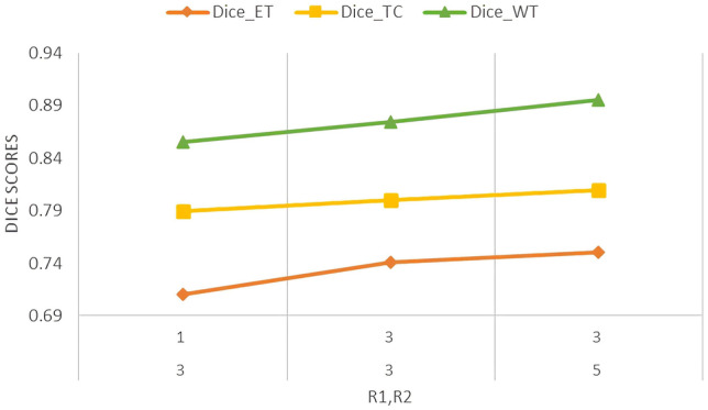
Line graph showing dice scores of ET, WT, and TC on different settings of r1 and r2

Effectiveness of Kernel Size and ML-KCNN Block

We also experimented on FCN-based architecture on instead of using MLKC block, just on the kernel of size 3 × 3, 5 × 5, and 7 × 7 is checked explicitly to observe the impact on their presence on the performance of the model and how their combined aggregation (known as multi-level approach) performance is different from single kernel size. It is observed that as the size of kernel increases, the performance significantly improves as it captures more information. The results show that the multi-level approach improved the segmentation performance. This shows the effectiveness of us expand and aggregate approach used in MLKC block (Fig. 10) (Table 4).

Fig. 10.

Graph of DSC results obtained by using different kernel size and ML-KCNN on FCN based architecture

Table 4.

Effect of using different kernel sizes and MLKC block on performance on BraTs 2019 validation dataset

Kernel size 3 × 3	Kernel size 5 × 5	Kernel size 7 × 7	Dice ET	Dice WT	Dice TC
✓			0.70	0.82	0.76
	✓		0.71	0.84	0.77
		✓	0.72	0.84	0.79
✓	✓	✓	0.74	0.87	0.81

Effectiveness of Loss Function

In our approach, we used GDL function, which is the multi-class extension of the dice loss function, where the weight of each class is inversely proportional to the square of label distributions. To compare the effect of GDL function on the performance of ML-KCNN, we compare it with weighted cross-entropy (WCE) loss function used for training. The qualitative results are shown in Table 5. It is observed that GDE shows better performance as compared to WCE. GDE loss tries to minimize the DSC and handles class imbalance issues [44].

Table 5.

Effectiveness of loss function on the BraTs 2019 segmentation dataset validation results

Loss Function	Dice ET	Dice WT	Dice TC
Weighted cross entropy	0.73	0.87	0.79
Generalized dice loss	0.74	0.88	0.81

Comparison of Segmentation Time on Test Data

We compare the effect of using Kronecker convolution on test time predictions with standard and dilated convolution. The experiments of test time predictions are shown in Table 6. It is noted that the running time of Kronecker convolution as compared to 3D convolution is 5 s more as compared to standard convolution because expanding the kernel size increases the computation time, and the average operation in Kronecker convolution increases the computational time as an extra operation performed before convolution but on the other hand reduces the number of parameters. Moreover, the post-processing technique increases the computational time to 30 to 40 s.

Table 6.

Comparison of segmentation time on test data predictions

Architecture	Time
FCN without MLKC block	10 to 15 s
Proposed MLKC	15 to 20 s
Proposed MLKC + post-processing	30 to 40 s

Conclusion

In this study, an architecture based on 3D Kronecker convolution named as ML-KCNN is proposed with multi-level paths to aggregate information at different levels. Furthermore, the post-processing technique that consists of combined CRF with CC helps to reduce the outliers and reduces the false positives from predictions. By covering the missing holes by atrous convolution, the receptive field size would be changed without using any extra parameters. Using a multi-level convolution block able to capture information at different levels that aggregate global and local information. For the evaluation of our proposed architecture, we have performed extensive experiments with varying evaluation metrics. For handling the class imbalance problem, we have used the generalized dice loss function. Our proposed architecture works well on real-time segmentation. Other segmentation tasks in medical imaging can also be solved using our proposed MLKCNN. We can also explore the different explainable model to make interpretable predictions.

Funding

This work has been supported by Higher Education Commission under Grant # 2(1064) and is carried out at Medical Imaging and Diagnostics (MID) Lab at COMSATS University Islamabad, under the umbrella of National Center of Artificial Intelligence (NCAI), Pakistan.

Declarations

Conflict of Interest

The authors declare no competing interests.

References

- 1.Louis, David N., et al: The 2016 World Health Organization classification of tumors of the central nervous system: a summary. Acta Neuropathologica 131.6:803–820,2016 [DOI] [PubMed]
- 2.Centers for Disease Control and Prevention: Data collection of primary central nervous system tumors. National Program of Cancer Registries Training Materials. Atlanta, Georgia: Department of Health and Human Services, Centers for Disease Control and Prevention, 2004
- 3.Brain Tumor - Diagnosis. 18 Mar. 2019, www.cancer.net/cancer-types/brain-tumor/diagnosis. Last Accessed: 25 April 2020
- 4.Galanaud, Damien, et al: Noninvasive diagnostic assessment of brain tumors using combined in vivo MR imaging and spectroscopy. Magnetic Resonance in Medicine: An Official Journal of the International Society for Magnetic Resonance in Medicine 55.6:1236–1245,2006 [DOI] [PubMed]
- 5.Rees J. Advances in magnetic resonance imaging of brain tumours. Current Opinion in Neurology. 2003;16(6):643–650. doi: 10.1097/00019052-200312000-00001. [DOI] [PubMed] [Google Scholar]
- 6.UCSF Department of Radiology & Biomedical Imaging. Exploring the Brain: Is CT or MRI Better for Brain Imaging? UCSF Radiology, 16 Nov. 2015, https://radiology.ucsf.edu/blog/neuroradiology/exploring-the-brain-is-ct-or-mri-better-for-brain-imaging
- 7.Menze BH, Jakab A, Bauer S, Kalpathy-Cramer J, Farahani K, Kirby J, et al: The Multimodal Brain Tumor Image Segmentation Benchmark (BRATS), IEEE Transactions on Medical Imaging 34(10):1993–2024,2015. 10.1109/TMI.2014.2377694 [DOI] [PMC free article] [PubMed]
- 8.Krizhevsky, Alex, Ilya Sutskever, and Geoffrey E. Hinton. Imagenet classification with deep convolutional neural networks. Advances in neural information processing systems. 2012.
- 9.Keçeli AS, Aydın K, Ahmet BC: Combining 2D and 3D deep models for action recognition with depth information. Signal, Image and Video Processing 12.6:1197–1205,2018
- 10.van Harten, Louis, et al: Automatic segmentation of organs at risk in thoracic CT scans by combining 2D and 3D convolutional neural networks. SegTHOR@ ISBI. 2019
- 11.Yu, Fisher, and Vladlen Koltun: Multi-scale context aggregation by dilated convolutions. arXiv preprint arXiv:1511.07122 2015
- 12.Wu, Tianyi, et al. Tree-structured kronecker convolutional network for semantic segmentation. 2019 IEEE International Conference on Multimedia and Expo (ICME). IEEE, 2019
- 13. Zheng S, Jayasumana S, Romera-Paredes B, Vineet V, Su S, Du D, Huang C, Torr PH: Conditional random fields as recurrent neural networks. In Proceedings of the IEEE International Conference on Computer Vision, 2015, pp 1529–1537
- 14.Peng C, et al: Large kernel matters—improve semantic segmentation by global convolutional network. Proceedings of the IEEE conference on computer vision and pattern recognition, 2017
- 15.Adams A, Baek J, Davis MA: Fast high-dimensional filtering using the permutohedral lattice. In Computer Graphics Forum, volume 29, pp 753–762. Wiley Online Library, 2010
- 16.Liu Z, Li X, Luo P, Loy C-C, Tang X: Semantic image segmentation via deep parsing network. In Proceedings of the IEEE International Conference on Computer Vision, 2015, pages 1377–1385
- 17.Lin G, Shen C, van den Hengel A, Reid I: Efficient piecewise training of deep structured models for semantic segmentation. In The IEEE Conference on Computer Vision and Pattern Recognition (CVPR), June 2016
- 18.Barron JT, Poole B: The fast bilateral solver. ECCV, 2016
- 19.Sudre CH, Li W, Vercauteren T, Ourselin S, Jorge Cardoso M: Generalised dice overlap as a deep learning loss function for highly unbalanced segmentations. In: Cardoso M. et al. (eds) Deep learning in medical image analysis and multimodal learning for clinical decision support. DLMIA 2017, ML-CDS 2017. Lecture Notes in Computer Science, vol 10553. Springer, Cham, 2017 [DOI] [PMC free article] [PubMed]
- 20.Sargur N. Srihari. Machine learning: generative and discriminative models. Cedar University of Befallo, University of Befallo, https://cedar.buffalo.edu/~srihari/CSE574/Discriminative-Generative.pdf
- 21.Lee C-H, et al: Segmenting brain tumors with conditional random fields and support vector machines. International Workshop on Computer Vision for Biomedical Image Applications. Springer, Berlin, Heidelberg, 2005
- 22.Bauer S, Nolte L-P, Reyes M: Fully automatic segmentation of brain tumor images using support vector machine classification in combination with hierarchical conditional random field regularization. international conference on medical image computing and computer-assisted intervention. Springer, Berlin, Heidelberg, 2011 [DOI] [PubMed]
- 23.He K, et al: Deep residual learning for image recognition. Proceedings of the IEEE conference on computer vision and pattern recognition, 2016
- 24.Long J, Shelhamer E, Darrell T: Fully convolutional networks for semantic segmentation. Proceedings of the IEEE conference on computer vision and pattern recognition, 2015 [DOI] [PubMed]
- 25.Mlynarski P, et al: 3D convolutional neural networks for tumor segmentation using long-range 2D context. Computerized Medical Imaging and Graphics 73:60–72,2019 [DOI] [PubMed]
- 26.Pereira S, et al: Adaptive feature recombination and recalibration for semantic segmentation with Fully Convolutional Networks. IEEE transactions on medical imaging, 2019 [DOI] [PubMed]
- 27.Chen H, et al: Brain tumor segmentation with deep convolutional symmetric neural network. Neurocomputing, 2019
- 28.Isensee F, et al: No new-net. International MICCAI Brainlesion Workshop. Springer, Cham, 2018
- 29.Xu, Hai, et al. Deep cascaded attention network for multi-task brain tumor segmentation. International Conference on Medical Image Computing and Computer-Assisted Intervention. Springer, Cham, 2019
- 30.Akil M, Saouli R, Kachouri R: Fully automatic brain tumor segmentation with deep learning-based selective attention using overlapping patches and multi-class weighted cross-entropy. Medical Image Analysis 101692,2020 [DOI] [PubMed]
- 31.Ding Yi, et al: A stacked multi-connection simple reducing net for brain tumor segmentation. IEEE Access 7:104011–104024,2019
- 32.Chen C, Liu X, Ding M, Zheng J, Li J: 3D Dilated multi-fiber network for real-time brain tumor segmentation in MRI. In: Shen D. et al Eds .Medical Image Computing and Computer Assisted Intervention – MICCAI 2019. MICCAI 2019. Lecture Notes in Computer Science, vol 11766. Springer, Cham, 2019
- 33.Rafi A et al: U-Net Based Glioblastoma Segmentation with Patient’s Overall Survival Prediction. International Symposium on Intelligent Computing Systems. Springer, Cham, 2020
- 34.Wang G, et al: Automatic brain tumor segmentation using convolutional neural networks with test-time augmentation. International MICCAI Brainlesion Workshop. Springer, Cham, 2018
- 35.Zhao X, et al: Brain tumor segmentation using a fully convolutional neural network with conditional random fields. International Workshop on Brainlesion: Glioma, Multiple Sclerosis, Stroke and Traumatic Brain Injuries. Springer, Cham, 2016
- 36.Wang F, Jiang R, Zheng L, Meng C, Biswal B: 3D U-Net based brain tumor segmentation and survival days prediction. In: Crimi A., Bakas S. (eds) Brainlesion: glioma, multiple sclerosis, stroke and traumatic brain injuries. BrainLes 2019. Lecture Notes in Computer Science, vol 11992. Springer, Cham, 2019
- 37.Hamghalamm M, Lei B, Wang T: Brain tumor synthetic segmentation in 3D multimodal MRI scans. arXiv preprint arXiv:1909.13640 2019
- 38.Agravat R, Raval MS: Brain tumor segmentation and survival prediction. arXiv preprint arXiv:1909.09399 2019
- 39.Amian M, Soltaninejad M: Multi-resolution 3D CNN for MRI brain tumor segmentation and survival prediction. arXiv preprint arXiv:1911.08388 2019
- 40.Murugesan GK, et al: Multidimensional and multiresolution ensemble networks for brain tumor segmentation. bioRxiv 760124,2019
- 41.Jiang Z, et al: Two-stage cascaded U-Net: 1st place solution to BraTS challenge 2019 segmentation task. International MICCAI Brainlesion Workshop. Springer, Cham, 2019
- 42.Vu MH, Nyholm T, Löfstedt T: TuNet: end-to-end hierarchical brain tumor segmentation using cascaded networks. arXiv preprint arXiv:1910.05338 2019
- 43.McKinley R, et al: Triplanar ensemble of 3D-to-2D CNNs with label-uncertainty for brain tumor segmentation. International MICCAI Brainlesion Workshop. Springer, Cham, 2019
- 44.Milletari F, Navab N, Ahmadi S-Ahmad: V-net: Fully convolutional neural networks for volumetric medical image segmentation. 2016 fourth international conference on 3D vision (3DV). IEEE, 2016
- 45.Bernal J, et al: Deep convolutional neural networks for brain image analysis on magnetic resonance imaging: a review. Artificial intelligence in medicine 95:64–81, 2019 [DOI] [PubMed]