Acquisition of murine splenic myeloid cells for protein and gene expression profiling by advanced flow cytometry and CITE-seq

Summary

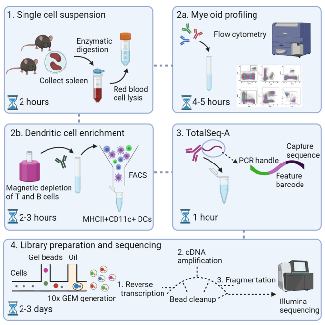
Here, we outline detailed protocols to isolate and profile murine splenic dendritic cells (DCs) through advanced flow cytometry of the myeloid compartment and single-cell transcriptomic profiling with integrated cell surface protein expression through CITE-seq. This protocol provides a general transferrable road map for different tissues and species.

For complete details on the use and execution of this protocol, please refer to Lukowski et al. (2021).

Graphical abstract

Highlights

• •Protocol to obtain integrated single-cell gene and protein expression data
• •Optimized flow cytometry panel for confident delineation of six main myeloid lineages
• •Gating strategy identifies large cell state heterogeneity within each lineage

Here, we outline detailed protocols to isolate and profile murine splenic dendritic cells (DCs) through advanced flow cytometry of the myeloid compartment and single-cell transcriptomic profiling with integrated cell surface protein expression through CITE-seq. This protocol provides a general transferrable road map for different tissues and species.

Before you begin

This protocol consists of two main workflows; (i) to acquire advanced flow cytometry data, and (ii) to acquire single cell transcriptomic data with integrated epitope detection (CITE-seq). For both workflows, the preparation of cell suspensions is a starting point. The workflow is exemplified using murine splenocytes with C57BL/6 background to delineate and isolate myeloid cells and dendritic cells (DCs). Experiments were carried out using female mice aged 6–12 weeks. All animal procedures and experiments were performed in compliance with the ethical guidelines of the National Health and Medical Research Council of Australia, with approval from the IMVS Animal Ethics Committee and the University of Queensland Animal Ethics Committee (UQDI/452/1).

Other tissue types (e.g., lymph node, skin), genetic backgrounds and species, as well as human clinical samples, may require species- or tissue-specific optimization of dissociation and choice of antibodies. A protocol that outlines the preparation of single cells from other murine tissue can be found here (Liu et al., 2020).

High-dimensional flow cytometry assays require expert knowledge that lie beyond the scope of this protocol, and principles for design and execution of advanced flow cytometry have been discussed elsewhere (Cossarizza et al., 2019; Dipiazza et al., 2019; Kalina, 2020; Liechti et al., 2021; Maciorowski et al., 2017; Mair and Tyznik, 2019; Wang and Hoffman, 2017).

CITE-seq is a rather young technology and resources to optimized protocols currently remain sparse. Useful resources regarding determining the optimal concentration of oligo-tagged antibodies can be found here (Mair et al., 2020; Buus et al., 2021).

Specific considerations

• 1.Due to differences in antibody batches and flow cytometer hardware components, the flow cytometry antibody panel presented here can only serve as guide, and should be optimized at each user lab. Re-titration of all antibodies is highly recommended to attain the best stain index for each antibody.
• 2.To allow confident discrimination of positive and negative cell populations in the flow cytometry workflow, we strongly encourage preparation of fluorescence minus one (FMO) controls.
• 3.Ensure antibodies used for cell sorting bind to different epitopes than CITE-seq oligo-tagged antibodies.
• 4.To validate and reduce background from oligo-tagged antibodies, we highly recommend titrating oligo-tagged antibodies using a dT-oligonucleotide tagged fluorescence dye and flow cytometry to determine optimal concentration.
• 5.Determine a target cell number before performing the CITE-seq protocol, and perform a mock sorting and antibody incubation, to inform yourself of required numbers of animals or samples, estimation of time from tissue collection to library preparation and protocol-associated cell loss.
• 6.Decide on a sequencing depth that is appropriate for your aim. The minimum recommendation from 10× Genomics is >20,000 reads per cell for gene expression libraries and 5,000 reads per cell for barcoded antibody libraries.

Preparation of solutions

Note: Recipes for all required solutions are outlined under materials and equipment

• 7.Prepare buffers required for preparation of single cell suspensions: PBS, digestion buffer, ACK lysis buffer.
• 8.Prepare solutions for flow cytometry: FACS buffer, compensation bead solution, Fc-block/FVS solution, antibody solution.
• 9.Prepare solutions for 10× Genomics Chromium workflow as described in the appropriate kit protocol or on the 10× Genomics website.

Key resources table

REAGENT or RESOURCE	SOURCE	IDENTIFIER
Antibodies
Anti-mouse CD11c PE-Dazzle (dilution 1:400)	BioLegend	Cat#117348; RRID: AB_2563655; Clone: N418
Anti-mouse CD11c PE-Cy7 (dilution 1:100)	BD Pharmingen	Cat#558079; RRID: AB_647251; Clone: HL3
Anti-mouse CD16/CD32 (Fc block) (dilution 1:100)	BioLegend	Cat# 101301; RRID: AB_312800; Clone: 93
Anti-mouse I-A/I-E APC-Cy7 (dilution 1:400)	BioLegend	Cat#107628; RRID: AB_2069377; Clone: M5/114.15.2
Anti-mouse TCRb Biotin (dilution 1:200)	BioLegend	Cat#109204; RRID: AB_313427; Clone: H57-597
Anti-mouse CD19 Biotin (dilution 1:200)	BioLegend	Cat#115504; RRID: AB_313639; Clone: 6D5
Anti-mouse CD45 BUV615 (dilution 1:1600)	BD Biosciences	Cat#751170; RRID: AB_2875194; Clone: 30-F11
Anti-mouse CD3 BV750 (dilution 1:100)	BioLegend	Cat# 100225; RRID: AB_10900444; Clone: 17A2
Anti-mouse CD19 BV570 (dilution 1:200)	BioLegend	Cat# 115535; RRID: AB_10933260; Clone: B4
Anti-mouse Ly6G BUV737 (dilution 1:100)	BD Biosciences	Cat# 741813; RRID: AB_2871151; Clone: 1A8
Anti-mouse PDCA1 APC (dilution 1:800)	BioLegend	Cat# 127015; RRID: AB_1967101; Clone:927
Anti-mouse CD11b APC-R700 (dilution 1:800)	BD Biosciences	Cat# 564985; RRID: AB_2739033; Clone: M1/70
Anti-mouse F4/80 PE-Cy5 (dilution 1:800)	BioLegend	Cat#123111; RRID: AB_893494; Clone: BM8
Anti-mouse Ly6C FITC (dilution 1:800)	BioLegend	Cat# 128005; RRID: AB_1186134; Clone: HK1.4
Anti-mouse I-A/I-E BV711 (dilution 1:800)	BioLegend	Cat# 107643; RRID: AB_2565976; Clone: M5/114.15.2
Anti-mouse CD11c BV421 (dilution 1:200)	BioLegend	Cat# 117329; RRID: AB_10897814; Clone: N418
Anti-mouse CD24 BV605 (dilution 1:100)	BioLegend	Cat# 101827; RRID: AB_2563464; Clone: M1/69
Anti-mouse XCR1 BV650 (dilution 1:100)	BioLegend	Cat# 148220; RRID: AB_2566410; Clone: ZET
Anti-mouse CD172A PerCP-eFluor710 (dilution 1:200)	Thermo Fisher Scientific	Cat# 46-1721-82; RRID: AB_10804639; Clone: P84
Anti-mouse CD4 BUV496 (dilution 1:200)	BD Biosciences	Cat# 612952; RRID: AB_2813886; Clone: GK1.5
Anti-mouse CD326 (Epcam) BUV394 (dilution 1:400)	BD Biosciences	Cat# 740281; RRID: AB_2740020; Clone:G8.8
Anti-mouse CD11c (Totalseq-A0106, GTTATGGACGCTTGC)	BioLegend	Cat#: 117355; RRID: AB_2750352; Clone: N418
Anti-mouse/ human CD11b (Totalseq-A0014, TGAAGGCTCATTTGT)	BioLegend	Cat#: 101265; RRID: AB_2734152; Clone: M1/70
Anti-mouse CD172a (Totalseq-A0422, GATTCCCTTGTAGCA)	BioLegend	Cat#: 144033; RRID: AB_2800670; Clone: P84
Anti-mouse CD370 (Totalseq-A0556, AACTCAGTTGTGCCG)	BioLegend	Custom-built; Part #: 96461; Clone: 7H11
Anti-mouse CD4 (Totalseq-A001, AACAAGACCCTTGAG)	BioLegend	Cat#: 100569; RRID: AB_2749956; Clone: RM4-5
Anti-mouse CD8a (Totalseq-A002, TACCCGTAATAGCGT)	BioLegend	Cat#: 100773; RRID: AB_2734151; Clone: 53-6.7
Anti-mouse F4/80 (Totalseq-A0114, TTAACTTCAGCCCGT)	BioLegend	Cat#: 123153; RRID: AB_2749986; Clone: BM8
Anti-mouse Siglec H (Totalseq-A0119, CCGCACCTACATTAG)	BioLegend	Cat#: 129615; RRID: AB_2750537; Clone: 551
Anti-mouse, rat XCR1 (Totalseq-A0568, TCCATTACCCACGTT)	BioLegend	Cat#: 148227; RRID: AB_2783120; Clone: ZET
Anti-mouse CD24 (Totalseq-A0212, TATATCTTTGCCGCA)	BioLegend	Cat#: 101841; RRID: AB_2750380; Clone: M1/69
Anti-mouse CD117 (Totalseq-A0012, TGCATGTCATCGGTG)	BioLegend	Cat#: 105843; RRID: AB_2749960; Clone: 2B8
Chemicals, peptides, and recombinant proteins
Collagenase D	Roche	11088858001
DNase	Roche	11284932001
Reagents according to Chromium protocol	https://assets.ctfassets.net/an68im79xiti/1W6c5yj7FAiBQdOKabc6sc/06e962ecdff018fb20b6979859cf1f5e/CG000317_ChromiumNextGEMSingleCell3-v3.1_CellSurfaceProtein_RevB.pdf	Various
Reagents according to CITE-seq protocol	Protocol - TotalSeq™-A Antibodies and Cell Hashing with 10x Single Cell 3' Reagent Kit v3 3.1 Protocol (BioLegend.com)	Various
Critical commercial assays
EasySep™ Mouse Streptavidin RapidSpheres™ Isolation Kit	STEMCELLTM Technologies	Cat#19860
LIVE/DEAD™ Fixable Aqua Dead Cell Stain Kit	Invitrogen	Cat#L34965
Fixable Viability Stain (FVS) 440UV (dilution 1:250)	BD Biosciences	Cat#566332
Brilliant Stain Buffer Plus	BD Biosciences	Cat#566385
Cell Staining Buffer	BioLegend	Cat#420201
Chromium Next GEM Single Cell 3ʹ Kit v3.1	10× Genomics	PN-1000268 or PN-1000269
Chromium Next GEM Chip G Single Cell Kit	10× Genomics	PN-1000120 or PN-1000127
Dual Index Kit TT Set A	10× Genomics	PN-1000215
Deposited data
Murine CITE-seq data	(Lukowski et al., 2021)	NCBI GEO GSE149544
Experimental models: Organisms/strains
Mus musculus C57BL/6J-Tg(HLA-A2/H2-K)6Scr/HsdArc	Animal Resources Center www.arc.wa.gov.au	Product code: A2KB
Oligonucleotides
AF647-dT [5'-5Alex647N-T30-3’]	IDT	N/A
Oligonucleotides according to CITE-seq protocol	BioLegend: https://www.BioLegend.com/en-us/protocols/totalseq-a-antibodies-and-cell-hashing-with-10x-single-cell-3-reagent-kit-v3-3-1-protocol	Various
Software and algorithms
Kaluza	Beckman Coulter	https://www.beckman.com.au/flow-cytometry/software/kaluza; RRID:SCR_016182;
bcl2fastq	Illumina	v2.20
Cellranger	10× Genomics	v6.0
Seurat	https://satijalab.org/seurat/	v3/v4
Other
Disposable transfer pipette	Copan	Cat#201CS01
FACS tube: Falcon® Round-Bottom Tubes with Cell Strainer Cap, 5 mL	Corning	Cat#352235
1.5 mL Eppendorf Tubes® 3810×	Eppendorf	Cat#0030125150
50 mL Falcon Tube	Corning	Cat#430290
BD 300800 Microlance Hypodermic Needle 23G × 1" Blue	GP Supplies	Cat#300800
BD 1 mL insulin syringe	BD	Cat#326719
Falcon® 70 μm Cell Strainer	Corning	Cat#352350
Corning® Costar® Stripette® serological pipettes	Corning	SKU: CLS4492-200EA
Bio-Rad TC20 Cell counter	Bio-Rad	Cat#1450102
Eppendorf 5810R centrifuge or centrifuge capable of holding FACS tube inserts	Eppendorf	5810000084
Pipettes and and pipette tips capable of 0.25 μL–1000 μL volumes	N/A	N/A
EasySepTM Magnet	STEMCELLTM Technologies	Cat#18000
BD FACSymphony A5 Flow Cytometer	BD	N/A
MoFlo Astrios Cell Sorter	Beckman Coulter	N/A
10× Genomics Chromium Controller	10× Genomics	N/A
Sequencing instrument (NextSeq/HiSeq/NovaSeq; single cell libraries not compatible with MiSeq)	Illumina	N/A
Fine scissors	N/A	N/A
Forceps	N/A	N/A
Equipment/consumables according to Chromium NextGEM single cell 3′ gene expression protocol, version 3.1 rev. B	10x Genomics: https://assets.ctfassets.net/an68im79xiti/1W6c5yj7FAiBQdOKabc6sc/06e962ecdff018fb20b6979859cf1f5e/CG000317_ChromiumNextGEMSingleCell3-v3.1_CellSurfaceProtein_RevB.pdf	Various
Equipment/consumables according to BioLegend CITE-seq protocol for TotalSeq-A antibodies and 10× Genomics Single Cell 3′ Reagent Kit v3.1	BioLegend: Protocol - TotalSeq™-A Antibodies and Cell Hashing with 10x Single Cell 3' Reagent Kit v3 3.1 Protocol (BioLegend.com)	Various

Materials and equipment

Phosphate-buffered saline (PBS)

Reagent	Final concentration	Final volume/amount
NaCl	137 mM	8g
KCl	2.7 mM	0.2 g
Na2HPO4	10 mM	1.44 g
KH2PO4	1.8 mM	0.24 g
H2O	N/A	1 L
Total	N/A	1 L

Note: Adjust PBS to pH 7.4. PBS can be stored at room temperature for 6 months, but should be prepared fresh for highly sensitive sequencing assays.

Digestion buffer

Reagent	Final concentration	Final volume
Collagenase D	1 mg/mL	5 μL
DNase I	0.1 mg/mL	10 μL
PBS	N/A	1 mL
Total	N/A	1 mL

Note: This solution should be prepared fresh.

Ammonium-chloride-potassium (ACK) lysis buffer

Reagent	Final concentration	Final volume/amount
NH4Cl	0.15 M	8.29 g
KHCO3	0.01 M	1 g
EDTA (0.5M pH 8.0)	0.1 mM	200 μL
Milli-Q purified water	N/A	1L
Total	N/A	1L

Note: Adjust ACK buffer to pH 7.2–7.4. ACK buffer can be stored at 4°C for up to 6 months, but should be prepared fresh for highly sensitive sequencing assays.

Compensation bead solution

Reagent	Final concentration	Final volume
Ultra eComp beads	30% (v/v)	120 μL (6 drops)
PBS	N/A	240 μL
Total	N/A	360 μL

Note: This solution should be prepared fresh.

FACS buffer

Reagent	Final concentration	Final volume
PBS	N/A	960 mL
EDTA (0.5M pH 8.0)	2 mM	4 mL
FBS	2%	20 mL
Total	N/A	1L

Note: FACS buffer can be stored at 4°C for up to 3 months for flow cytometry assays,but should be prepared fresh for highly sensitive sequencing assays.

Fc-block/FVS solution

Reagent	Final concentration	Final volume/amount
PBS	N/A	N/A
Fc block	5 μg/mL	0.25 μg
FVS440UV	40 μg/mL	2 μg
Total	N/A	50 μL

Note: Fc-block/FVS solution should be prepared fresh on the day of experiment. Upscale for samples >1. The amount of reagents has been determined based on a cell number of 2–5 × 10⁶ cells in a total staining volume of 50 μL. The volume of PBS depends on the required volume of antibody, and should lead to a total volume of 50 μl.

Antibody solution

Reagent	Final concentration	Final volume/amount
FACS buffer	N/A	N/A
Epcam-BUV395	0.5 μg/mL	0.025 μg
CD4-BUV496	1 μg/mL	0.05 μg
CD45-BUV615	0.125 μg/mL	0.00625 μg
Ly6G-BUV737	2 μg/mL	0.1 μg
CD11c-BV421	1 μg/mL	0.05 μg
CD19-BV570	0.5 μg/mL	0.025 μg
CD24-BV605	2 μg/mL	0.1 μg
XCR1-BV650	2 μg/mL	0.1 μg
MHCII∗-BV711	0.25 μg/mL	0.0125 μg
CD3-BV750	2 μg/mL	0.1 μg
CD64-BV786	2 μg/mL	0.1 μg
Ly6C-FITC	0.625 μg/mL	0.03125 μg
CD712a-PerCP-eFluor710	1 μg/mL	0.05 μg
F4/80-PE/Cy5	0.25 μg/mL	0.0125 μg
PDCA1-APC	0.25 μg/mL	0.0125 μg
CD11b-APC-R700	0.25 μg/mL	0.0125 μg
Total		50 μL

Note: Antibody solution should be prepared fresh on the day of experiment. Upscale for samples >1. The antibody amount has been determined based on a cell number of 2–5 × 10⁶ cells in a total staining volume of 50 μL. The volume of FACS buffer depends on the required volume of antibody, and should lead to a total volume of 50 μl. ∗The MHCII antibody depends on the murine genetic background. We here used an I-A/I-E-specific antibody that is compatible with C57BL/6J mice.

Computer requirements

For 10× Genomics cell ranger

8-core Intel or AMD processor (16 cores recommended)

64GB RAM (128GB recommended)

1TB free disk space

64-bit CentOS/RedHat 6.0 or Ubuntu 12.04

For high performance computing (HPC) cluster mode

8-core Intel or AMD processor per node

6GB RAM per core

Shared filesystem (e.g. NFS)

SGE or LSF batch scheduling system

Step-by-step method details

Spleen collection

Timing: 30 min

This section describes euthanasia and collection of spleens from mouse.

• 1.Use healthy, 6–12 weeks old mice.
• 2.Euthanize mice using an institutionally approved method (e.g., CO₂ asphyxiation).
• 3.Place the mouse right side down on the dissection mat, and spray fur with 80% ethanol to disinfect.
• 4.Using blunt forceps and scissors, make a 1.5 cm horizontal incision in the skin on the left thorax just below the ribcage.
• 5.Dissect further through peritoneum until the spleen is visible (dark red bean-shaped organ of approximately 1 cm length).
• 6.To avoid tearing and potential cell loss/ damage, carefully grasp the spleen with the forceps, lift it out of the abdomen and ensure complete detachment from the pancreas.
• 7.Dislodge spleen by cutting the splenic blood vessels with fine scissors. Some bleeding is normal.
• 8.Using forceps, place spleen into 1.5 mL Eppendorf tube containing 1 mL of cold PBS, and store on ice.
• 9.Dispose of the mouse cadaver.

Preparation of single cell splenocytes

Timing: 90 min

This section describes the preparation of murine splenic single cell suspensions.

• 10.Remove the spleen from PBS using blunt forceps and place into a fresh Eppendorf tube.
• 11.Using a 22-gauge needle and 1 mL syringe, inject 1 mL of collagenase D (Col/D) Digestion Buffer at 18°C–23°C into each spleen, using multiple puncture locations to ensure Col/D reaches all parts of the tissue. The tissue typically inflates in this process, and excess digestion buffer will leak into the tube. Spleen will then be incubated immersed in digestion buffer.
• 12.Incubate spleen immersed in digestion buffer in Eppendorf tube in a 37°C water bath for 30 min.

Note: The choice of digestion enzyme can impact the antigen density on the cell surface of cells, and can therefore interfere with ability to detect antigens using flow cytometry and CITE-seq. Col/D works well in regard to detection of the antigens described in this protocol, and users should test the effects of digestion on the detection of antigens should other antibodies be used.

Note: During cell digestion, complete the bead-based single stain compensation controls (see next section).

• 13.Transfer contents of the splenic digestion onto a 70 μm cell strainer over a 50 mL Falcon tube and gently mash the spleen through the strainer using a rubber plunger of a 5 mL syringe.
• 14.Wash strainer with 10 mL of PBS at 18°C–23°C using a 10 mL serological pipette.
• 15.Centrifuge splenocytes at 300 × g for 10 min at 4°C.
• 16.Decant the supernatant and resuspend cells of 1 spleen in 1 mL of Ammonium-Chloride-Potassium (ACK) lysis buffer and incubate on ice for 2 min.

Note: Only one spleen should be processed through one cell strainer to ensure maximal cell yield. If multiple spleens need to be combined, cells should be pooled after Step 19.

CRITICAL: Do not let cells incubate in ACK lysis buffer for longer than 2 min as this can negatively impact cell yield and viability.

• 17.Add 10 mL PBS and centrifuge at 300 × g for 10 min at 4°C.
• 18.Decant supernatant and resuspend cells of one spleen (approximately 50 × 10⁶ cells) in 1 mL of PBS.
• 19.If absolute cell counts are required, resuspend 20 μL of unstained cells in 20 μL trypan blue, transfer to counting slide, and count.

Note: If cell viability of splenocytes is below 80%, PBS in digestion buffer and washes can be replaced by plain RPMI1640 media.

• 20.For flow cytometry workflow proceed to step 21, for CITE-seq workflow proceed to step 59.

Flow cytometry compensation controls

Timing: 30 min

This section describes the preparation of compensation controls for flow cytometry.

Note: Due to overlapping emission spectra of diverse fluorochromes, a spill over of fluorescence from the primary to the secondary detector is common for certain combinations of fluorochromes, and needs to be corrected in a process termed compensation. The accuracy of compensation is paramount to distinguish positive and negative signals, and therefore requires special attention. The topic of compensation can be explored in detail elsewhere (Cossarizza et al., 2019). The protocol here uses beads to acquire compensation controls, while other protocols might suggest using cells as single-color controls. Each of these methods has disadvantages which should be considered on the basis of the experiment.

• 21.Vortex compensation beads for 30 s to break up aggregates.
• 22.Pipette 20 μL of bead solution to empty FACS tubes, followed by 80 μL of FACS buffer.

Note: The manufacturer recommends to use one drop (approx. 20 μL) of beads per single stain control, however we have found that beads can be diluted in FACS buffer in up to a 1:3 dilution.

• 23.Pipette 1 μL of the corresponding antibody to each tube.
• 24.Incubate on ice or at 4°C in the dark for 15 min.
• 25.Add 1 mL of FACS buffer.
• 26.Centrifuge at 300 × g for 5 min at 4°C.
• 27.Carefully decant supernatant.
• 28.Resuspend in 200 μL of FACS buffer.
• 29.Keep compensation controls on ice or at 4°C in the dark until acquisition.

Flow cytometry sample antibody staining

Timing: 2 h

This section describes the incubation of single cells with fluorescence-tagged antibodies.

CRITICAL: Advanced flow cytometry require a deep understanding of the technology including panel design based on antigen-density, spectral overlap, spreading errors, compensation and downstream data analysis that lie beyond the scope of this protocol. New users to flow cytometry are strongly encouraged to seek expert advice, mentoring and training by their flow cytometry facility before commencing experiments. Useful additional resources can be found here: (Cossarizza et al., 2019; Brummelman et al., 2019; Mair and Tyznik, 2019).

CRITICAL: All antibodies and buffers should be kept on ice while preparing antibody solutions. Antibody solutions should be prepared fresh within the hour of sample incubation to minimise chances for antibody interaction, and kept shielded from light.

Note: A complete list of antibodies to immunophenotype splenic myeloid cells is provided in Table 1. This panel was developed and optimised based on a similar panel developed by (Dipiazza et al., 2019). The panel can be extended, and channels that are suitable for the addition of antibodies which detect functional features are indicated. Antibody concentrations can be found under materials and equipment.

Table 1.

Configuration table of murine myeloid antibody panel for BD FACSymphony A5

Laser	Filter	Feature	Fluorochrome
355 nm (UV)	UV_379/28	Epcam (optional)	BUV395
	UV_450/50	FVS	440UV
	UV_515/30	CD4	BUV496
	UV_586/15	Functional	BUV563
	UV_610/20	CD45	BUV615
	UV_740/35	Ly6G	BUV737
405 nm (Violet)	V_450/50	CD11c	BV421
	V_586/15	CD19	BV570
	V_610/20	CD24	BV605
	V_670/30	XCR1	BV650
	V_710/50	MHC II	BV711
	V_740/35	CD3	BV750
	V_780/60	CD64	BV786
488 nm (Blue)	B_515/20	Ly6C	FITC
	B_610/20	Functional	PE/Dazzle
	B_710/50	CD172A	PerCP eFluor710
	B_780/60	Functional	PE/Cy7
561 nm (Yellow/Green)	YG_670/30	F4/80	PE/Cy5
642 nm (Red)	R_670/30	PDCA-1	APC
	R_710/50	CD11b	APC-R700

• 30.Pipette approximately 5 × 10⁶ splenocytes into FACS tubes for the unstained sample and each experimental sample tube, and 2 × 10⁶ splenocytes into a live/dead single stain control tube.

Note: Falcon® 5 mL Round Bottom Polystyrene tubes work well to retain myeloid cells, and allow the addition of sufficient volumes of FACS buffer for washing steps.

Note: Alternative to a cell-based single cell control for live-dead stain, amine-reactive compensation beads can be used here. The stain index of these beads can be improved by dilution in PBS and incubation at 18°C–23°C to encourage the covalent binding reaction.

• 31.Keep unstained sample on ice or at 4°C until acquisition.
• 32.Transfer half of live/dead single stain cells into a fresh Eppendorf tube and put on a heat plate set at 50°C for 10 min to initiate cell death.
• 33.During incubation time, prepare a Fc block/FVS solution as outlined in materials and equipment.
• 34.After 10 min, place dead cells on ice for 2 min, then transfer back to original live/dead Eppendorf tube containing live cells.
• 35.Centrifuge live/dead single stain and experimental sample tubes at 300 × g for 5 min at 4°C.
• 36.Decant supernatant.
• 37.Add 50 μL of live/dead/Fc-block cocktail to experimental samples and live/dead single stain.

CRITICAL: Live/dead labelling must be performed in PBS only. The presence of FCS in FACS buffer will bind live/dead reagent and interfere with live/dead staining of splenocytes.

• 38.Incubate on ice or at 4°C in the dark for 15 min.
• 39.During incubation time prepare antibody cocktail using the desired concentration of each antibody in 40 μL FACS buffer + 10 μL Brilliant Stain buffer per experimental sample (upscale according to number of experimental samples plus 10%, see antibody cocktail constituent table in materials and equipment).

Note: The antibody concentrations provided in this protocol are optimized for a cell number of 5 × 10⁶ cells which are stained in a final volume of 50 μL. Because antibody binding depends on the cell number, cell density and antibody density, both volume and antibody need to be adjusted with any change in cell numbers.

Note: Brilliant Stain Buffer should be used if more than one BD Brilliant dye is used to prevent non-specific polymer interactions. 10 μL of Brilliant Stain Buffer should be added to the antibody cocktail for each experimental sample.

CRITICAL: To distinguish specific staining from abnormalities derived from fluorescence spillover, spreading error and cell-type specific autofluorescence, fluorescence minus one (FMO) controls should be included (Mair and Tyznik, 2019). These controls are especially critical when measuring features with low to medium antigen density and a clear bimodal expression pattern (expressed and not expressed) is not expected.

• 40.Add 1 mL of PBS to all tubes incubated with live/dead/Fc-block cocktail, and centrifuge at 300 × g for 5 min at 4°C.
• 41.Decant supernatant.

Note: Using a smooth ‘invert-pour-tab-revert’ movement, pour supernatant followed by a brief and gentle tab to paper towel to absorb remaining liquid. Cell pellets are routinely not disturbed by this action.

• 42.Resuspend live/dead single stain control in 400 μL of FACS buffer and leave on ice or at 4°C in the dark until acquisition.
• 43.Resuspend experimental samples each in 50 μL of antibody cocktail.
• 44.Incubate samples on ice or at 4°C in the dark for 20 min.
• 45.Add 1 mL FACS buffer and centrifuge at 300 × g for 5 min at 4°C.
• 46.Decant supernatants.
• 47.Resuspend cell pellets in 400 μL of FACS buffer store on ice or at 4°C in the dark until acquisition.

Note: Once stained, unfixed experimental samples should be acquired within 2 h to ensure viability, and avoid fluorochrome degradation.

CRITICAL: This protocol has not been tested with fixation reagents. Any method of fixation, should be tested prior as fixation can negatively affect tandem fluorophores. If fixation is required, compensation controls also need to be treated with fixation agents, and the user should refer to fixation protocols (Cossarizza et al., 2019).

Flow cytometry data acquisition

Timing: ∼2 h

This section describes a basic workflow to acquire cells using a BD FACSymphony A5 flow cytometer.

CRITICAL: Flow cytometers should only be operated by trained users. Detailed guidelines for optimal instrument set up have been discussed elsewhere (Mair and Tyznik, 2019), and users of this protocol will need to be familiar with these processes, or have their samples acquired by professional instrument operators.

• 48.Vortex and strain cells through a FACS tube microstrainer using a disposable transfer pipette immediately before loading onto cytometer.
• 49.Using unstained cells, manipulate PMT voltages to adjust forward and side scatter (FSC/SSC), and reflect 3 times of the robust standard deviation (rSD) for each channel in order to ensure comparable fluorophore sensitivity across all channels (Wang and Hoffman, 2017).

Note: Using 3 × rSD to set PMT voltages reliably approximates appropriate signal detection while reducing electronic noise. However, for dim signals, a range of up to 10 × rSD is recommended (Cossarizza et al., 2019). Manipulated rSD values should be derived from pre-gated lymphocytes using the forward and side scatter gate.

• 50.After setting voltages, begin acquisition of single stain compensation controls, beginning with the unstained sample according to the automatic compensation workflow instructions of your specific cytometer.
• 51.Vortex compensation tubes for 3–5 s to resuspend beads before acquisition.
• 52.Acquire 5000 total events for each compensation control.

Note: Successful automatic compensation depends on a sufficiently high stain index of the compensation controls, that optimally is larger than the stain index of the antibody in the sample. Bead-based compensation controls typically provide a high stain index, but can at times for yet unknown reasons lead to overcompensation (Brummelman et al., 2019).

• 53.Following compensation control acquisition, perform automatic compensation calculation.
• 54.Vortex experimental samples before acquisition to ensure cells are in solution. Acquire at least 2 × 10⁶ events of FSC/SSC lymphocyte gate of each experimental sample for adequate resolution.
• 55.Export flow cytometry standard (FCS) files.

Flow cytometry data analysis

Timing: ∼4–8 h

This section describes a basic workflow to carry out quality control of the acquired flow cytometry data and the delineation of the myeloid cells in murine spleen. The steps below give a guideline to analyze flow cytometric data using Kaluza software (Beckman Coulter, version 3.1). Other software are available and the principles for data analysis remain the same.

• 56.
  Verify and correct automatic compensation if required.

  CRITICAL: The success of the automatic compensation algorithms depends on multiple factors, and can under circumstances lead to over- and undercompensation. A very careful quality control of the compensation matrix is essential before commencing any data analysis. This compensation quality control should only be carried out by highly experienced flow cytometry experts, who have an in-depth understanding of fluorochrome spill over, spreading errors and the effects of cell-type specific autofluorescence. If a manual modification to the algorithm-based compensation is required, this too should only be attempted by experts in the field, and is prone to subjectivity-derived error.

  Achieving accurate algorithm-based compensation can be challenging and might require comparison of bead- and cell-based compensation controls (Liechti and Roederer, 2019), and if differences are observed, cell-based compensation controls should be considered as biologically relevant gold standard (Cossarizza et al., 2019). Working forward with either a falsely algorithm-based or a falsely manually corrected compensation has major implications to the data analysis and interpretation of data. The steps outlined below provide a basic NxN (every parameter against every parameter) approach how to quality check the compensation and attempt correction.

  • a.
    Import FCS files to the analysis software of choice.
  • b.
    To omit debris and isolate lymphocytes, generate a FSC-A/SCC-A bivariate plot, and gate populations of interest (Figure 2A).
  • c.
    To omit doublets, generate a FSC-A/FSC-H bivariate plot, and gate events in a linear, 45 degree line (Figure 2A).
  • d.
    Create a bivariate plot for each used channel, with the channel on the X axis.
  • e.
    Highlight all plots and change the Y axes to the first channel.
  • f.
    If typical patterns that suggest overcompensation (“super-negative” events) or undercompensation (“leaning” triangular populations) are observed, correct compensation as required (see example provided in Figure 1).
  • g.
    Change Y axes to the next channel and repeat compensation correction.
  • h.
    Repeat for all channels.

    Note: We find that when a manual compensation is required, the complete NxN approach should be carried out at least twice, or until a full round of NxN can be completed without further modifications are needed. This can be laborious but is critical to the quality of data.

  • i.
    Apply corrected compensation to all experimental samples.

• 57.Identify myeloid cells based on gating strategy demonstrated in Figures 2 and 3. Begin by isolating live, single, leukocytes, and then excluding non-target populations such as T-cells (CD3+), and B-cells (CD19+).

Note: Identical gating strategy should be applied to all experimental samples. However, when analyzing samples of different origins (eg. unstimulated versus stimulated, or spleen versus lymph node), the expression level of features can differ, and gate limits should be chosen to include these differences.

• 58.Export statistics (cell numbers, percentages, median fluorescence intensity (MFI) data) for significance testing.

Figure 2.

Flow cytometry gating strategy for a 16-color murine myeloid panel

Splenocytes of C57BL/6 mice were incubated with fluorochrome-conjugated antibodies and analyzed by flow cytometry. Red boxes indicate final target populations.

(A) CD45+ leukocytes were identified after exclusion of debris, doublet discrimination and exclusion of dead cells.

(B) From CD45+ cells, B cells and NKT/T cells were excluded, and Ly6G+ neutrophils were validated based on CD11b expression. pDCs were identified as PDCA1+. From PDCA1- cells, macrophages were delineated based on expression of F4/80 and absence of Ly6C- and CD11c-.

(C) Monocytes were identified from CD3-CD19-Ly6G-PDCA1- cells as Ly6C+, and monocyte diversity was further identified through differential expression of CD11b and CD172a.

(D) cDCs were identified from CD3-CD19-Ly6G-PDCA1-Ly6C- cells based on expression of MHC-II+ and CD11c+. cDCs were subdivided into cDC1 (XCR1+CD172a-) and cDC2 (CD172a+XCR1-) cells, and their identity was verified by expression of CD24 and CD11b, respectively. cDC1 and cDC2 cells were further subdivided into CD4+ and CD4- cells.

Figure 1.

Compensation of fluorochrome spill over

Compensation using bead-based single-color controls can lead to over- and undercompensation in a cell-based sample, which requires manual correction.

Figure 3.

Representative flow cytometry gating tree for delineating murine myeloid cells in spleen

Enrichment of myeloid cells

Timing: 20 min

This section describes magnetic bead enrichment of myeloid cells using a negative isolation of non-T and non-B cells, with the aim to reduce sorting time and thus increase cell viability post sorting. The following steps are in accordance with the manufacturer’s protocol (EasySep™ Mouse Streptavidin RapidSpheres™ Isolation Kit).

Note: We pooled splenocytes of 6 C57BL/6 mice, and used 2 × 10⁸ splenocytes for myeloid cell enrichment. This allowed us to subsequently sort ∼50,000 DCs.

• 59.Resuspend splenocytes at 1 × 10⁸ cells/mL in FACS buffer in a round bottomed 5 mL tube.
• 60.Add 5 μL/mL of biotin conjugated anti-TCRb and biotin conjugated 5 μL/mL anti-CD19 to the cell solution.
• 61.Incubate for 10 min at 18°C–23°C.
• 62.Add 75 μL of RapidSpheres^TM magnetic beads and incubate for 2.5 min at 18°C–23°C.
• 63.Place the tube in an EasySep^TM magnet and incubate for 2.5 min.
• 64.Carefully decant the supernatant with the myeloid cells into a new FACS tube.

Fluorescent activated cell sorting (FACS)

Timing: ∼2 h

This section is to isolate DCs to high purity using FACS. This reduces the levels of debris, doublets and unwanted cells for downstream sequencing.

CRITICAL: Cell sorting requires highly trained staff and should be carried out optimally by a flow cytometry core facility.

• 65.Use all enriched cells from the previous step, set aside a small quantity of cells for unstained and single stain controls for compensation. Single stain controls can alternatively be bead-based as described in the section flow cytometry compensation controls.
• 66.Stain cells with Fc-block (1:100) and live/dead cell stain (1:250) for 20 min on ice.
• 67.Wash with 1 mL PBS and centrifuge at 300 × g for 5 min at 4°C.
• 68.Resuspend pellet with anti-MHCII-APC-Cy7 (1:400) and anti-CD11c-PE-Cy7 (1:200) in 500 μL FACS buffer and incubate for 20 min on ice.

CRITICAL: If oligo-tagged antibodies for CITE-seq overlap with antibodies used for sorting, a different antibody clone needs to used. For antibody staining of CD11c, we used the clone HL3 for sorting, and the clone N418 for CITE-seq.

• 69.Wash cells with 3 mL FACS buffer, centrifuge at 300 × g for 5 min at 4°C and resuspend in 1 mL FACS buffer
• 70.
  Set up cell sorter PMT voltages and compensation using unstained and single stained cells.

  • a.
    Determine cells and eliminate debris with FCS-H vs SSC-H.
  • b.
    Determine single cells with FSC-A vs FSC-H and SSC-A vs SSC-H.
  • c.
    Determine live cells as live/dead stain negative.
  • d.
    Determine cDCs as MHCII+CD11c+.
• 71.Sort cells into FACS tube containing 500 μL 100% FCS.
• 72.Dilute with 2 mL FACS buffer and centrifuge at 300 × g for 5 min at 4°C.

Note: Record a small fraction of the sorted cells to check post sort purity and viability (Figure 4).

Figure 4.

DC sorting

Myeloid enriched splenocytes were incubated with live/dead stain, Fc-block and antibodies against CD11c and MHCII. DCs were sorted as alive single CD11c+MHCII+ cells to a purity >90%.

Incubation of DCs with nucleotide barcoded antibodies

Timing: 1 h

Here, cells are stained with oligo-tagged antibodies that are conjugated with nucleotide sequences specific for each antibody. The steps listed below are in accordance with BioLegend CITE-seq protocol for TotalSeq-A antibodies and 10× Genomics Single Cell 3′ Reagent Kit v3.1 (https://www.biolegend.com/en-us/protocols/totalseq-a-antibodies-and-cell-hashing-with-10x-single-cell-3-reagent-kit-v3-3-1-protocol).

• 73.Resuspend cell pellet from the sort in Cell Staining Buffer (1 ×10ˆ⁶mouse cells in 49.5 μL) in a FACS tube.
• 74.Add 0.5 μL of TruStain FcX™ PLUS (anti-mouse CD16/32) antibody per 49.5 μL cell suspension and incubate for 10 min at 4°C.
• 75.Prepare antibody pool using titrated amount (up to 1 μg of each TotalSeq-A antibody). Add Cell Staining Buffer to make the volume of the antibody pool 50 μL for each 50 μL cell suspension.
• 76.To remove antibody aggregates, centrifuge the antibody pool at 1,400 × g for 10 min at 4°C and carefully pipette out the antibody pool without touching the bottom of the tube.
• 77.Add the 50 μL of antibody pool to each 50 μL of cell suspension.
• 78.Incubate for 30 min on ice.
• 79.Wash with 3 mL Cell Staining Buffer and centrifuge at 400 × g for 5 min at 4°C.
• 80.Decant supernatant.
• 81.Repeat wash twice.
• 82.Resuspend cell pellet in 250 μL Cell Staining Buffer and immediately move to the next step.

Note: Antibody validation and titration should be performed prior to carrying out this protocol. It is possible to titrate the oligo-tagged antibodies using either single cell sequencing read outs (https://www.biolegend.com/en-us/blog/titrating-totalseq-antibodies), which is costly, or by flow cytometry using the same clone with a fluorophore or dT-oligonucleotide tagged fluorescent dye. An example of oligo-tagged antibody validation at a concentration of 0.5 μg and using a dT-oligonucleotide tagged fluorescent dye is shown in Figure 5. However, because sequencing is more sensitive than flow cytometry, the optimal antibody concentration for flow cytometry might not be the optimal antibody concentration for sequencing. The accurate identification of the optimal antibody concentration without the need for sequencing represents a current limitation to the technology.

Optional: According to the 10× Genomics protocol for Cell Surface Protein Labelling, cells can be stained with oligo-tagged antibodies simultaneously with fluorochrome conjugated antibodies prior to sorting (https://support.10xgenomics.com/single-cell-gene-expression/overview/doc/demonstrated-protocol-cell-surface-protein-labeling-for-single-cell-rna-sequencing-protocols). Staining prior to sorting can have advantages: it may reduce the number of unbound oligo-tagged antibodies as the cells will be washed multiple times in the sorting process; and reduce the time between cell isolation and downstream steps, thus reducing the time until cell lysis. However, this requires staining a higher number of cells and the amount of oligo-tagged antibodies needs to be adjusted accordingly.

Optional: To distinguish oligo-tagged antibody specific binding and background noise, users can consider a spike-in of cells that are negative for the antibody-specific epitopes. For example, for CITE-seq experiments of murine cells, users can spike in human cells. This provides an internal control for antibody background noise. Alternatively, if a diverse population of cells is processed, cells that are considered negative for epitope expression can be used to determine background (Lukowski et al., 2021).

CRITICAL: Wash thoroughly after oligo-tagged antibody staining to reduce background noise from unbound antibodies.

Figure 5.

Total-Seq-A antibody validation

Splenocytes were incubated with flow cytometry live-dead stain, Fc-block and antibodies against MHCII and CD11c, and each Total-Seq-A antibody which was conjugated to a dT-oligonucleotide tagged fluorescence dye. Flow cytometry and Total-Seq-A antibodies against CD11c were specific to different epitopes.

10× chromium platform and library preparation

Timing: 1.5 days

This step includes generating gel beads in emulsions (GEMs), barcoding, cDNA amplification and library construction.

Note: Due to Chromium kit updates that have occurred since the original study (Lukowski et al., 2021), the instructions and resources outlined below differ slightly from what was performed at the time. We describe below the current best-practice workflow, using the most updated kits available, as a recommendation for how we would conduct the experiment today.

Note: Single cell sequencing experiments are highly technical and expensive to perform. If you are inexperienced with single cell library preparation and sequencing, or there are aspects that will be performed by a core facility, we advise discussing your project in advance with the facility or with 10× Genomics technical support. Understanding the requirements and key points at each step of the protocol will give the best chance for a successful outcome.

CRITICAL: The Chromium library preparation protocol is required to be performed in a timely manner once cells are ready. It is imperative that the relevant protocols and user guides have been read thoroughly and are familiar to the user before beginning, and all necessary reagents and consumables have been acquired and prepared in advance.

• 83.Prepare all necessary reagents for GEM generation as outlined in the 10× Genomics Chromium User Guide (https://assets.ctfassets.net/an68im79xiti/1W6c5yj7FAiBQdOKabc6sc/06e962ecdff018fb20b6979859cf1f5e/CG000317_ChromiumNextGEMSingleCell3-v3.1_CellSurfaceProtein_RevB.pdf).
• 84.Manually count cells and ensure that cell viability is above 80%
• 85.For super-loading of the Chromium reaction (targeting more than 10,000 cells per reaction), consult the table on page 33 of the Cell Multiplexing User Guide (https://assets.ctfassets.net/an68im79xiti/Ic17bUxh3yu95BmBNGsE3/3d333cebd76782ed1ccf8a032bb3e294/CG000388_ChromiumNextGEMSingleCell3-v3.1_CellMultiplexing_Rev_A.pdf) to determine the appropriate volume of cells to add for a particular concentration. For example, to target 15,000 single cells would require ∼27.5uL of a cell suspension at a concentration of 1 × 10⁶ cells/mL.
• 86.Prepare gene expression and CITE-seq libraries by following the steps outlined in the BioLegend TotalSeq-A protocol (https://www.BioLegend.com/en-us/protocols/totalseq-a-antibodies-and-cell-hashing-with-10x-single-cell-3-reagent-kit-v3-3-1-protocol) and the 10x Genomics Chromium User Guide (https://assets.ctfassets.net/an68im79xiti/1W6c5yj7FAiBQdOKabc6sc/06e962ecdff018fb20b6979859cf1f5e/CG000317_ChromiumNextGEMSingleCell3-v3.1_CellSurfaceProtein_RevB.pdf).

Note: Start GEM generation immediately after oligo-tagged antibody staining to minimize cell death. It is recommended that the viability of the samples at this point is >80%. Using low-viability samples can impact data quality due to increased ambient RNA from dead and dying cells.

CRITICAL: Ensure that you are following the TotalSeq-A protocol to include ADT additive primer in the cDNA amplification mix, and save the low molecular weight fragments in the supernatant of the post-amplification clean-up, otherwise a CITE-seq library will not be able to be generated for your sample.

Pause point: Purified full-length amplified cDNA (including CITE-seq cDNA) and final libraries can both be stored at −20^oC until moving forward to library preparation or sequencing, respectively.

Note: To reduce the possibility of index cross-talk, if possible avoid using the following combinations of CITE-seq indexes with samples intended for the same sequencing run:

- RPI01 and RPI09

- RPI08 and RPI12

The above index combinations have a Sequence-Levenshtein edit distance of 2. All other combinations of CITE-seq (RPI01 to RPI12) and Chromium (SI-TT-A1 to SI-TT-H12) indexes have an edit distance of >=3, allowing for accurate correction of a single base mismatch caused by substitution, insertion or deletion. If the pairs noted above must be used together, it would be preferable to adjust the default parameters during fastq generation to allow no mismatches.

Note: Both 10× Genomics and BioLegend will periodically provide version updates for the protocols cited above. The documents in this protocol are the latest versions at time of writing; you may want to check to confirm you are using the most up-to-date protocol available before starting your experiment, as subsequent updates may improve performance and outcomes.

Illumina sequencing

Timing: 1 day

This section generates sequencing data from the prepared gene expression and CITE-seq libraries.

• 87.Pool libraries and sequence according to desired sequencing depth. For the antibody pool used here, we recommend pooling the CITE-seq and gene expression libraries for each sample at a 10% and 90% molar ratio respectively. When sequencing two samples targeting 15,000 cells each with this pooling, you can expect to generate >20,000 gene expression reads per cell (the minimum recommended by 10× Genomics) using a NovaSeq SP 100 cycle sequencing run. Sequencing kits can be scaled up as needed for projects with greater sample numbers. For projects utilizing higher numbers of antibodies, it will be necessary to increase the pooling proportion of the CITE-seq libraries accordingly to ensure adequate read numbers for each antibody used. The minimum recommended sequencing depth for 10× Genomics gene expression libraries is 20,000 reads per cell and 5,000 reads per cell for barcoded antibody (CITE-seq) libraries. It is important to note that if the number of barcoded antibodies increases significantly or includes highly abundant proteins such as CD45, the read depth per cell may require adjustment.

Note: Pooled CITE-seq/gene expression libraries can be run using the recommended configuration of Read1 – 28bases, Index1 – 10bases, Index2 – 10bases, Read2 – 90 bases.

Data pre-processing

Timing: 1 day

This section includes initial data pre-processing using Cell Ranger software to generate fastq files for each sample and count tables containing both gene expression and CITE-seq feature information.

• 88.Raw sequencing data from the Illumina platform is in the BCL format. These raw files must be demultiplexed into individual samples and subsequently converted to fastq files. This can be achieved using the 10× Genomics Cell Ranger mkfastq pipeline in conjunction with the sample-specific index barcodes. Follow the instructions for running the Cell Ranger mkfastq pipeline found on the 10× Genomics support site: https://support.10xgenomics.com/single-cell-gene-expression/software/pipelines/latest/using/mkfastq.
• 89.Cell Ranger mkfastq requires a comma-separated table with columns specifying the flowcell lane, sample names and indexes used. It is possible to process multiple library types at once, which avoids the need to run mkfastq once for each library type. However some modifications to the recommended SimpleCSV samplesheet are required. In this modification, the CITE-seq library indexes can be presented in the SimpleCSV samplesheet in a dual-index format. To do this, add ‘ATCT’ (the four bases immediately following the 6 bp index in the adaptor sequence) to the end of each index sequence, then provide the sequence ‘GTGTAGATCT’ in an additional ‘Index2’ column. This will be the sequence generated from single-indexed CITE-seq library fragments by the i5 index primer. The 10× dual index TT Set A ID can be replicated in both ‘Index’ and ‘Index2’ columns for the gene expression libraries. Please see example below for generating fastq files for samples using RPI01 (ATCACG) and RPI02 (CGATGT) CITE-seq indexes, for samples run on a NovaSeq6000 platform with v1.5 kits.

Lane,Sample,Index,Index2

∗,CDC_WT,SI-TT-A1,SI-TT-A1

∗,CS_CDC_WT,ATCACGATCT,GTGTAGATCT

∗,CDC_BATF3_KO,SI-TT-A2,SI-TT-A2

∗,CS_CDC_BATF3_KO,CGATGTATCT,GTGTAGATCT

Note: The exemplary samples CDC_WT and CDC_BATF3_KO were sorted cDCs from wildtype and Batf3−/− mice published in (Lukowski et al., 2021).

• 90.Using the fastq files generated in Step 1, follow the instructions for running the Cell Ranger count pipeline with feature barcoding, which utilizes Cell Ranger Feature Barcoding capabilities to incorporate the CITE-seq information in the output gene-count matrix: https://support.10xgenomics.com/single-cell-gene-expression/software/pipelines/latest/using/feature-bc-analysis.
• 91.The reference genomes and annotations for mouse (GRCm38) and human (GRCh38) required for Cell Ranger count can be obtained from the 10× Genomics website, or can be provided by the user.
• 92.Following the generation of sample-level count matrices by Cell Ranger count, multiple samples can be combined into a single large matrix using Cell Ranger aggr (aggregate). It is also possible to analyze each sample individually without the use of the aggregate function.
• 93.After count matrix aggregation, the dataset comprising gene and protein expression values is ready for analysis in Seurat or other software.

Note: The strand read by the i5 sequencing primer depends on the sequencing platform used. The index2 sequence presented above is for sequencers using a ‘reverse complement’ workflow for dual-indexing, as for NovaSeq6000 with v1.5 kits. The index2 sequence should be modified to use the reverse complement if a ‘forward strand’ workflow is used, for example on a NovaSeq6000 with v1.0 kits.

Note: If single-indexed gene expression libraries are generated (with SI-GA-xx index IDs), a SimpleCSV with a single index column is sufficient. In this case, to accommodate an 8bp i7 index read, the suffix ‘AT’ can be added to the CITE-seq indexes. The SimpleCSV for the same example as above would then look like this:

Lane,Sample,Index

∗,CDC_WT,SI-GA-A1

∗,CS_CDC_WT,ATCACGAT

∗,CDC_BATF3_KO,SI-GA-A2

∗,CS_CDC_BATF3_KO,CGATGTAT

Expected outcomes

This protocol outlines a general workflow and critical considerations for phenotyping of cells using advanced flow cytometry, cell isolation using fluorescence-activated cell sorting and single cell sequencing of epitopes and transcripts. Specifically, we demonstrate the step-by-step methodology using murine splenocytes and antibodies to delineate, isolate and sequence myeloid cells and DCs.

The expected outcomes of the flow cytometric delineation of myeloid cells are shown in detail in Figures 2 and 3. The 16-color flow cytometry panel allows delineation of 5 main myeloid lineages, including monocytes, macrophages, neutrophils, pDCs and cDC cells, and a large cell subset and cell state heterogeneity within these main lineages. Our manual analysis allowed identification of 16 discrete populations, and additional cell state diversity is revealed when using unbiased bioinformatic approaches to identify heterogeneity based on differential co-expression of phenotypic features (Figure 6).

Figure 6.

Expected outcome of a bioinformatic unbiased analysis of the 16-color murine myeloid flow cytometry panel

(A) Single alive CD45+ CD3- CD19- cells were subjected to bioinformatic FlowSOM analysis based on expression of Ly6G, Ly6C, PDCA1, CD11b, CD11c, F4/80, MHCII, CD172a, CD24, XCR1, and CD4 with a metacluster number of 40. User-determined thresholds for positive signal were applied to all features. The analysis identified 40 distinct clusters of cells.

(B) Clusters were annotated based on key myeloid lineage features.

Expected outcomes of the CITE-seq workflow is a single cell sequencing dataset of approximately 25,000 DCs with a sequencing depth of 20,000 reads per cells (gene expression) and 5,000 reads per cell (barcoded antibodies).

Quantification and statistical analysis

For the flow cytometric analysis of myeloid cells, absolute numbers and relative abundances of myeloid cell lineages and cell states can be compared between different genotypes and treatment regimes. Differences in the mean fluorescence intensities of features with functional implications such as MHCII, CD64 and XCR1 can also be compared. For comparisons of functional feature expression, a fluorescence minus one (FMO) control should be included and the MFI of FMO should be subtracted to control for population-specific spreading errors and autofluorescence. In addition to traditional manual population gating, flow cytometry data can be analyzed using unbiased bioinformatic platforms (Melsen et al., 2020; Brummelman et al., 2019), and both should be used hand-in-hand to uncover cell lineage and cell state heterogeneity.

CITE-seq data can be analyzed using standard single cell bioinformatic workflows, such as Seurat (Butler et al., 2018) or Scanpy (Wolf et al., 2018). Examples of integrated analysis platforms for multi-omic data are weighted-nearest neighbor analysis (Hao et al., 2021), One-SENSE (Cheng et al., 2016; Mair et al., 2020), CiteFuse (Kim et al., 2020) and CITE-sort (Lian et al., 2020).

Limitations

Flow cytometry data is especially difficult to standardize between different laboratories due to differences in the hardware components of the cytometer as well as differences in batches of antibodies. The user will therefore have to re-titrate antibodies and establish optimal cytometer settings to achieve good data outcomes. Manual correction of the compensation is prone to user subjectivity and should be handled with extreme caution. A very detailed quality control of the algorithm-based compensation performed by the flow cytometer is absolutely essential. If the algorithm-based compensation does not successfully apply to the experimental samples, the user should aim to optimize the preparation and acquisition of the compensation controls to circumvent the need for a manual correction. Key principles to achieve this are outlined here (Cossarizza et al., 2019). Furthermore, spreading error needs to be investigated on individual cytometers to avoid false positive cell annotation. Acquisition of a complete set of FMO controls is laborious but will aid confident discrimination of positive and negative signals. We urge new flow cytometry users to study the current literature regarding advanced flow cytometry methodology guidelines (Mair and Tyznik, 2019) and recommended guidelines for flow cytometry reporting in detail (Lucas et al., 2020; Cossarizza et al., 2019), and advise that this is not a trivial methodology.

CITE-seq data may contain high levels of background noise from the barcoded antibody staining. This may be due to non-specific binding or high staining concentration, and antibody concentration optimization may help to reduce this noise. Of note, the current version of the protocol is optimized for cell surface proteins only. Concerning per-cell read depth, antibody panels designed to capture highly abundant proteins such as CD45 are likely to require deeper sequencing than the suggested depth. Since highly expressed proteins will account for a large proportion of sequencing reads in a given run, it is crucial to ensure the sequencing depth is sufficient to capture the real expression profile of lower expressed proteins. Overcoming this may require resequencing of the same CITE-seq library.

Troubleshooting

Problem 1

Lack of positive flow cytometry bead staining

Potential solution

Ensure the isotypes of the antibodies match those of rat, mouse, or hamster (steps 21–23). While eComp beads (Thermofisher) contain beads of all three isotypes, other commercial beads such as those provided by BD may not contain the isotype compatible with your antibodies.

Problem 2

Unclear discrimination of positive and negative signals.

Potential solution

FMO controls where the marker of interest is omitted from the antibody cocktail, and isotype controls can provide more accurate discrimination of positive staining (Maciorowski et al., 2017; Maecker and Trotter, 2006). Optimally FMO, controls should be acquired for every antibody, but this can be laborious (step 39). These controls however are essential for detection of antigens that are expressed at low to medium levels and a bimodal expression profile does not apply. The use of isotype controls which control only for binding of antibodies via Fc receptors is considered non-essential when Fc receptors are efficiently blocked before antibody staining. Internal negative controls (cells within the sample that don’t express the feature) can help with confident discrimination of expression, although these should have a comparable autofluorescence.

Problem 3

Low antibody staining

Potential solution

Absence of signal may be due to either absence of protein expression or of low photomultiplier tube (PMT) voltages (step 49). Low PMT voltages may cause insufficient filter sensitivity for receiving positive signals. Accurate setting of PMT voltages using an unstained sample combined with using antibody concentrations determined from titrations typically overcomes this problem. The PMT voltage can be increased to up to 10× rSD to detect dim signals, and should be accompanied by an FMO control. Furthermore, use of rainbow beads (BD) to set PMT voltages offers a quick and accurate method for consistent voltage setting over time (Kalina, 2020; Perfetto et al., 2006; Wang and Hoffman, 2017).

Problem 4

Inaccuracy in automatic compensation

Potential solution

High parameter compensation matrices are complex and require great care in creation. All downstream data analysis depends on the quality of compensation, and accurate compensation therefore is absolute paramount to any flow cytometry experiment (step 56). Optimally, all compensation controls, including the control of the viability stain, are acquired based on both cells and beads, and the performance of the algorithm-based compensation is compared. If differences in the spill-over values are observed between cells and beads, then cells are to be used as biologically relevant gold standard single color controls (Cossarizza et al., 2019). Of note, beads provided by different suppliers can vary in their capacity to achieve accurate algorithm-based compensation. Further, the stain index of all compensation controls should be higher than that of the antibody staining in the experimental sample, although this is not absolute. If still experiencing problems that the algorithm-based compensation leads to over- or under-compensation, only a highly trained and experienced user should attempt a manual correction using considerations of spill over, spreading error and co-expression. Compensation strategies have been described in detail by others (Szalóki and Goda, 2015; Maciorowski et al., 2017).

Resource availability

Lead contact

Further information and requests for resources and reagents should be directed to and will be fulfilled by the lead contact Janin Chandra, j.chandra@uq.edu.au.

Materials availability

This study did not generate new unique reagents.

Data and code availability

The flow cytometry data sets supporting this protocol, and used in Figures, have not been deposited in a public repository but are available from the corresponding author upon request. The Gene Expression Omnibus (GEO) accession number for the CITE sequencing data reported in this article is GEO: GSE149544 (https://www.ncbi.nlm.nih.gov/geo/query/acc.cgi?acc=GSE149544).

References

- Brummelman J., Haftmann C., Nunez N.G., Alvisi G., Mazza E.M.C., Becher B., Lugli E. Development, application and computational analysis of high-dimensional fluorescent antibody panels for single-cell flow cytometry. Nat. Protoc. 2019;14:1946–1969. doi: 10.1038/s41596-019-0166-2. [DOI] [PubMed] [Google Scholar]
- Butler A., Hoffman P., Smibert P., Papalexi E., Satija R. Integrating single-cell transcriptomic data across different conditions, technologies, and species. Nat. Biotechnol. 2018;36:411–420. doi: 10.1038/nbt.4096. [DOI] [PMC free article] [PubMed] [Google Scholar]
- Buus T.B., Herrera A., Ivanova E., Mimitou E., Cheng A., Herati R.S., Papagiannakopoulos T., Smibert P., Odum N., Koralov S.B. Improving oligo-conjugated antibody signal in multimodal single-cell analysis. Elife. 2021;10:e61973. doi: 10.7554/eLife.61973. [DOI] [PMC free article] [PubMed] [Google Scholar]
- Cheng Y., Wong M.T., Van Der Maaten L., Newell E.W. Categorical analysis of human T cell heterogeneity with one-dimensional soli-expression by nonlinear stochastic embedding. J. Immunol. 2016;196:924–932. doi: 10.4049/jimmunol.1501928. [DOI] [PMC free article] [PubMed] [Google Scholar]
- Cossarizza A., Chang H.D., Radbruch A., Acs A., Adam D., Adam-Klages S., Agace W.W., Aghaeepour N., Akdis M., Allez M. Guidelines for the use of flow cytometry and cell sorting in immunological studies (second edition) Eur. J. Immunol. 2019;49:1457–1973. doi: 10.1002/eji.201970107. [DOI] [PMC free article] [PubMed] [Google Scholar]
- Dipiazza A.T., Hill J.P., Graham B.S., Ruckwardt T.J. OMIP-061: 20-color flow cytometry panel for high-dimensional characterization of murine antigen-presenting cells. Cytometry A. 2019;95:1226–1230. doi: 10.1002/cyto.a.23880. [DOI] [PubMed] [Google Scholar]
- Hao Y., Hao S., Andersen-Nissen E., Mauck W.M., 3rd, Zheng S., Butler A., Lee M.J., Wilk A.J., Darby C., Zager M. Integrated analysis of multimodal single-cell data. Cell. 2021;184:3573–3587 e29. doi: 10.1016/j.cell.2021.04.048. [DOI] [PMC free article] [PubMed] [Google Scholar]
- Kalina T. Reproducibility of flow cytometry through standardization: Opportunities and challenges. Cytometry A. 2020;97:137–147. doi: 10.1002/cyto.a.23901. [DOI] [PubMed] [Google Scholar]
- Kim H.J., Lin Y., Geddes T.A., Yang J.Y.H., Yang P. CiteFuse enables multi-modal analysis of CITE-seq data. Bioinformatics. 2020;36:4137–4143. doi: 10.1093/bioinformatics/btaa282. [DOI] [PubMed] [Google Scholar]
- Lian Q., Xin H., Ma J., Konnikova L., Chen W., Gu J., Chen K. Artificial-cell-type aware cell-type classification in CITE-seq. Bioinformatics. 2020;36:i542–i550. doi: 10.1093/bioinformatics/btaa467. [DOI] [PMC free article] [PubMed] [Google Scholar]
- Liechti T., Roederer M. OMIP-060: 30-parameter flow cytometry panel to assess T cell effector functions and regulatory T cells. Cytometry A. 2019;95:1129–1134. doi: 10.1002/cyto.a.23853. [DOI] [PubMed] [Google Scholar]
- Liechti T., Weber L.M., Ashhurst T.M., Stanley N., Prlic M., Van Gassen S., Mair F. An updated guide for the perplexed: cytometry in the high-dimensional era. Nat Immunol. 2021 doi: 10.1038/s41590-021-01006-z. [DOI] [PubMed] [Google Scholar]
- Liu Z., Gu Y., Shin A., Zhang S., Ginhoux F. Analysis of myeloid cells in mouse tissues with flow cytometry. STAR Protoc. 2020;1:100029. doi: 10.1016/j.xpro.2020.100029. [DOI] [PMC free article] [PubMed] [Google Scholar]
- Lucas F., Gil-Pulido J., Lamacchia J., Preffer F., Wallace P.K., Lopez P. MiSet RFC standards: defining a universal minimum set of standards required for reproducibility and rigor in research flow cytometry experiments. Cytometry A. 2020;97:148–155. doi: 10.1002/cyto.a.23940. [DOI] [PubMed] [Google Scholar]
- Lukowski S.W., Rodahl I., Kelly S., Yu M., Gotley J., Zhou C., Millard S., Andersen S.B., Christ A.N., Belz G. Absence of Batf3 reveals a new dimension of cell state heterogeneity within conventional dendritic cells. iScience. 2021;24:102402. doi: 10.1016/j.isci.2021.102402. [DOI] [PMC free article] [PubMed] [Google Scholar]
- Maciorowski Z., Chattopadhyay P.K., Jain P. Basic multicolor flow cytometry. Curr. Protoc. Immunol. 2017;117:5.4.1–5.4.38. doi: 10.1002/cpim.26. [DOI] [PubMed] [Google Scholar]
- Maecker H.T., Trotter J. Flow cytometry controls, instrument setup, and the determination of positivity. Cytometry A. 2006;69:1037–1042. doi: 10.1002/cyto.a.20333. [DOI] [PubMed] [Google Scholar]
- Mair F., Erickson J.R., Voillet V., Simoni Y., Bi T., Tyznik A.J., Martin J., Gottardo R., Newell E.W., Prlic M. A targeted multi-omic analysis approach measures protein expression and low-abundance transcripts on the single-cell level. Cell Rep. 2020;31:107499. doi: 10.1016/j.celrep.2020.03.063. [DOI] [PMC free article] [PubMed] [Google Scholar]
- Mair F., Tyznik A.J. High-dimensional immunophenotyping with fluorescence-based cytometry: a practical guidebook. Methods Mol. Biol. 2019;2032:1–29. doi: 10.1007/978-1-4939-9650-6_1. [DOI] [PubMed] [Google Scholar]
- Melsen J.E., Van Ostaijen-Ten Dam M.M., Lankester A.C., Schilham M.W., Van Den Akker E.B. A comprehensive workflow for applying single-cell clustering and pseudotime analysis to flow cytometry data. J. Immunol. 2020;205:864–871. doi: 10.4049/jimmunol.1901530. [DOI] [PubMed] [Google Scholar]
- Perfetto S.P., Ambrozak D., Nguyen R., Chattopadhyay P., Roederer M. Quality assurance for polychromatic flow cytometry. Nat. Protoc. 2006;1:1522–1530. doi: 10.1038/nprot.2006.250. [DOI] [PubMed] [Google Scholar]
- Szalóki G., Goda K. Compensation in multicolor flow cytometry. Cytometry A. 2015;87:982–985. doi: 10.1002/cyto.a.22736. [DOI] [PubMed] [Google Scholar]
- Wang L., Hoffman R.A. Standardization, calibration, and control in flow cytometry. Curr. Protoc. Cytom. 2017;79:1.3.1–1.3.27. doi: 10.1002/cpcy.14. [DOI] [PubMed] [Google Scholar]
- Wolf F.A., Angerer P., Theis F.J. SCANPY: large-scale single-cell gene expression data analysis. Genome Biol. 2018;19:15. doi: 10.1186/s13059-017-1382-0. [DOI] [PMC free article] [PubMed] [Google Scholar]
Associated Data
This section collects any data citations, data availability statements, or supplementary materials included in this article.
Data Availability Statement